Additive and Multiplicative Noise Driven Systems in 1 + 1 Dimensions: Waiting Time Extraction of Nucleation Rates
Abstract
We study the rate of true vacuum bubble nucleation numerically for a field system coupled to a source of thermal noise. We compare in detail the cases of additive and multiplicative noise. We pay special attention to the choice of initial field configuration, showing the advantages of a version of the quenching technique. We advocate a new method of extracting the nucleation time scale that employs the full distribution of nucleation times. Large data samples are needed to study the initial state configuration choice and to extract nucleation times to good precision. The 1+1 dimensional models afford large statistics samples in reasonable running times. We find that for both additive and multiplicative models, nucleation time distributions are well fit by a waiting time, or gamma, distribution for all parameters studied. The nucleation rates are a factor three or more slower for the multiplicative compared to the additive models with the same dimensionless parameter choices. Both cases lead to high confidence level linear fits of plots, in agreement with semiclassical nucleation rate predictions.
I Introduction
In 1969 Langer [1] gave a first-principles formalism for calculating the decay rates of metastable states which was applicable to many types of nucleation and growth processes. Several limiting cases were discussed, including those of a small energy difference between the two phases and overdamped and underdamped systems. Vacuum stability in scalar field theory was discussed by Lee and Wick [2]in 1974. In contemporaneous work, the cosmological consequences of the decay of metastable vacuum states were investigated by Zel’dovich, Kobzarev, and Okun [3] and was further developed by Voloshin, Kobzarev, and Okun [4]. These authors investigated the idea of bubbles of a true vacuum phase nucleating and expanding in a phase of the false vacuum. In 1981 Guth [5] proposed that sufficient supercooling of the false vacuum before its decay could lead to enough exponential growth of the scale factor (inflation) to solve the flatness and homogeneity problems. This idea has itself undergone significant evolution ever since.
A formalism for calculating nucleation rates, first using semiclassical methods and then including quantum corrections, was worked out by Coleman [6] and Coleman and Callan [7] in 1977. It was in these latter works that a Lorentz-invariant account of tunneling was given. This technique uses a finite-action classical field configuration in Euclidean space, called the bounce. The bounce solution is the solution which minimizes the action. They also demonstrated how to treat zero modes in the decay rate calculation as well as how to determine the critical size of fluctuations which lead to bubbles that grow. In 1983 Linde [8] generalized the study to finite temperatures.
Calculation of decay rates involve solving the equation of motion of the scalar field. For the types of potentials which give rise to metastable vacuum states, the equations of motion are non-linear in the field and, unless severe approximations are made, analytic solutions cannot be found. The detailed out-of equilibrium, time dependent aspects of metastable vacuum decay can only be studied through numerical techniques. False vacuum decay at finite temperature has been studied numerically through the use of Langevin equations [9][10][11][12]. In these works the stochastic term in the Langevin equation was in the form of additive noise, a field independent, white noise driving term. Theoretical work [13][14][15] [16], however, suggest that the noise term may be more complicated and in general may be multiplicative and colored. We apply our study of Langevin dynamics to the range of parameters appropriate to the semiclassical regime, where there is reason to believe it makes sense[10][17]. This way we can be sure about the conclusions drawn from our new nucleation time method and about the comparison between the the additive and multiplicative noise models.
We study numerically the decay of the false vacuum in dimensions, focusing on the question of bubble nucleation rate. We consider in detail the effects of two different types of noise terms: additive, where the nucleation rate has been studied before[10] in dimensions, and multiplicative, which has not been studied in numerical detail in this context. Working in one spacial dimension affords several advantages: the system is theoretically simple, with renormalization not an issue, for example [18]; the extraction of the nucleation time scale by the new method we advocate requires generation of large data samples that can be achieved in reasonable times in a dimensional system; this simple system allows us to explore relatively quickly the influence of initial state configuration choice on nucleation time distribution; the good statistics allows us to make a sharp comparison between the results generated with our exploratory probe of the multiplicative model and those generated with the additive model.
Given our objective we are immediately confronted by the question of the proper definition of nucleation time. In order to make full use of the nucleation time data generated with each choice of input parameters (temperature, asymmetry parameter, driving amplitude and viscosity coefficient), we propose a new description of nucleation time based on a classic waiting time distribution ‡‡‡An exponential decay can be fitted to the tails of our distributions, but this would be misleading, as we discuss in Sections 4 and 5 . With this description of the distribution of nucleation times from the simulation data, we extract characteristic decay times for each parameter set. We find that the relationship between nucleation time and temperature, derived from semiclassical calculations, are reproduced by both Langevin models. We also find that nucleation times are systematically a factor of three or more longer in multiplicative noise models than in additive models, given the same values of scaled input parameters and the same initial state preparation in both models.
In the next section, we briefly review the ideas of vacuum transition in zero and non-zero temperature cases. In Section 3 we describe our numerical methods, including the preparation of the initial state of the field. In Section 4 we describe our procedure for fitting our data and extracting nucleation rates and present our results. In Section 5 we discuss our results and draw conclusions and comment on open questions. Three appendices provide further details and supporting data for material presented in the text.
II Quick Review of Nucleation Rates
Consider a self-interacting scalar field theory and suppose the field starts off with a value , which corresponds to the metastable minimum of the effective potential (hereafter referred to as the potential). Classically, transition to the global minimum at is forbidden, but there is a non-zero probability for quantum tunneling through the barrier with bubbles of the true vacuum appearing in the metastable phase. The decay probability per unit volume can be expressed by the functional integral[6][7]
| (1) |
where is the Euclidean action,
| (2) |
The equation of motion is
| (3) |
Notice the positive sign in front of the term on the right. This is the equation of motion of the field in the potential , exemplified in Fig. 1. Now the boundary conditions have to be suitably chosen. The field starts off at in the inverted potential and gets to the escape point . In the case of degenerate minima the path integral is dominated by the non-trivial minimum energy solution of the equation of motion, the instanton[19][20]. For non-degenerate minima the non-tivial solution to the equation of motion in Euclidean space corresponds to the field starting at the unstable minimum, , at , ’bouncing’ off the escape point at and asymptotically approaching again, as , the bounce solution. Semi-classically, the path integral in Eqn. 1 gives the tunneling rate per unit volume as,
| (4) |
where is the action, Eqn. 2, evaluated with the solution of the equation of motion with boundary conditions . The coefficient A contains quantum corrections to the tunneling rate. In most cases it is not possible to solve the equation of motion analytically with the appropriate boundary conditions. However there are limiting cases [1][6] where exact analytic solutions can be found. It was shown [21] that the spherically symmetric, , invariant bounce is the one with the least action. Then with the boundary conditions for the symmetric bounce the general solution for is of the so-called kink form
| (5) |
where and is the thickness of the transition region. This solution, valid when the difference between the energy density in the true vacuum and that in the false vacuum is small[6], is called the thin wall solution and the general form is depicted in Fig. 2. As the name of the approximation suggests, there is a sharp transition region (or thin wall) between the true and false vacuum phases. The interpretation of Fig. 2 is that somewhere in space, at , a bubble of the true vacuum, , is formed. Away from the center of the bubble there is a transition region, which is very narrow on the thin wall approximation. Beyond this transition region, and in particular as , the field is in the false vacuum state . The parameter appearing in Eqn. 5 is the radius of a critical size bubble which can be easily calculated in the thin wall approximation.
Tunneling at finite temperature can be studied using all of the above formalism if one uses the imaginary time technique of Matsubara [22], exploiting the equivalence between four dimensional field theory at finite temperature and Euclidean field theory in four dimensions with periodicity or anti-periodicity in one of the dimensions. The period is where . One therefore has the requirement that . For sufficiently high temperatures this additional condition gives the finite temperature action
| (6) |
where is the three dimensional Euclidean action and is the temperature. Eqn. 6 is valid at sufficiently high temperatures, higher than the temperature at which the period, , of the bounce solution is equal the critical radius, , of a bubble[8]. The solution to the equation of motion with the least action is now symmetric and the equation of motion can be solved in the thin wall approximation as above.
III Numerical Studies and Time Evolution
The theory of false vacuum decay outlined in the preceding section made clear that nucleation can be studied analytically only in a few limiting cases. Out of equilibrium time evolution properties can only be studied in detail using numerical techniques. Nucleation has been studied numerically through the use of Langevin equations. Early calculations, for example[10], used a Langevin equation for the time evolution of the field based solely on phenomenological grounds. Other studies have attempted to derive Langevin type equations from quantum field theory in the semiclassical limit. Typically the high frequency modes are treated as the thermal bath for the low frequency modes, which is identified as “the system”[14][15][23].
For a scalar field theory in one space and one time dimension, a phenomenological Langevin type equation can be written as,
| (7) |
where is a random force term originating from the coupling of the field to a thermal bath. The thermal noise term, , and the viscosity, , are related through the fluctuation dissipation theorem[24][25][18],
| (8) |
Since Eqn. 8 is central to our work and is used, but seldom discussed, in the field theory literature, we provide details on its implementation and its interpretation in our study in Appendix A. The appearance of the viscosity, , in the equations of motion and its relation to the thermal fluctuations through Eqn. 8 can be understood by considering the example of Brownian motion. A Brownian particle suspended in a fluid is subjected to random, microscopic, short-duration forces which, over a longer period of time, change the macroscopic velocity of the particle. At the same time the random forces in the direction opposite to the velocity of the particle serve to retard its motion. The very forces, therefore, that are responsible for the macroscopic motion of the suspended particle also are the ones that inhibit the motion, namely give rise to the viscosity of the medium. In order to include both effects of the random forces, two independent terms are introduced in the equation of motion; they are connected through the fluctuation-dissipation relation.
In Eqn. 7 the fluctuation term is linear. This is referred to as additive noise. However there is no reason why one should not consider a general case where the noise is non-linear. For example, a Langevin equation with a non-linear thermal fluctuation term has been derived, in a set of approximations [14], by considering a self interacting quantum scalar field. It was shown that, at finite temperature, if the short wavelength modes of the field are separated out and the two-loop effective potential is used, then the effective action contains imaginary terms which are interpreted as coming from Gaussian integrations over auxiliary fields, . These auxiliary fields appear in the the equation of motion in the form of a random fluctuation term. We adopt a phenomenological version of this result in a dimensional multiplicative noise model to discover what features of the nucleation rate may differ from those of the additive noise case.
| (9) |
Notice that there is now a non-linear viscosity coefficient. In the high temperature limit the fluctuation-dissipation relation, Eqn. 8, is valid[14].
We use the Langevin equations with linear and non-linear noise terms, and with the usual fluctuation-dissipation theorem to compare the effects of these types of noise on nucleation. This is the first such numerical study, as far as we know.
We re-scale the equations so that all parameters appearing in them are dimensionless. We give the detail of the re-scaling in appendix B. We propagate the solution of the equation of motion using a staggered leap-frog method[26]. We have checked that the results do not depend on this method. We also repeated simulation runs on a lattice twice as large as the one reported here to check that the results show no finite volume (or in 1-dimension finite length) effects. We use a lattice of size with a space step-size of and a time step of and with periodic boundary conditions. The value of the field at the time step in terms of the values at and , and at position on the lattice is given, for the additive model, Eqn. 7, by
| (10) |
where,
| (11) |
and
| (12) |
Gaussian white noise is used for both the linear(additive) and non-linear(multiplicative) couplings to the thermal bath. We relate the noise and viscosity through Equation 8. The discrete form of this equation is
| (13) |
where the and terms are introduced to compensate for the lack of dimensionality of the Kroneker deltas. is given by
| (14) |
where is a Gaussian random number generator of width one. The delta correlation is implemented by using a different random kick at each time and at each point on the lattice. By looking at approximately 100 bubble profiles we found that fluctuations which take the field at five contiguous lattice sites to the true vacuum value always grew to fill the entire lattice. Therefore we chose this criterion to determine when a bubble was formed.
A Initial Conditions
The initial conditions in such a numerical study have to be carefully chosen. We looked at nucleation times with random, uncorrelated initial field values distributed on the lattice. We also looked at nucleation times with short distance correlated and Gaussian distributed initial field values. We found that with the first case there was a long delay time during which no bubbles were formed. After this delay time there was a distribution of nucleation times rather sharply peaked around some value. With the second set of initial conditions, i.e. correlated and Gaussian distributed, we found that this delay time was sharply reduced, the distribution rising quickly and peaking much earlier. This is illustrated for samples of 5,000 bubbles in Fig. 5.
The initial field values, whose correlations and distributions are described by Figs. 3 and 4 are obtained using a quenching technique[27]. The effect of this initial state preparation on the bubble nucleation times is shown by the data indicated by the histogram on the left in Fig. 5. We scatter random field values on the lattice and propagate the solution of the equation of motion in a potential with only one minimum. We ensure that the curvature at the bottom of the potential closely matches the curvature of the asymmetric double well of interest. After some time the field acquires the thermal distribution with the desired short distance correlation. At this point, which is in the simulation, the potential is quenched, i.e., the asymmetric potential is switched on. Nucleation times are recorded with reference to this time. Fig. 4 shows the distribution of initial conditions just before quenching for both additive noise and multiplicative noise.
Summarizing, we find that when the initial state is not prepared by the quenching method just described, and random, uncorrelated, initial field values are placed on the lattice, there is a long delay time for the first bubble to appear, after which a peaked distribution of times develops. The delay time apparently corresponds to the time needed for the field to become correlated. Preparing the initial state so that it is correlated as shown in Figs. 3 and 4, produces the change in the distributions illustrated in Fig. 5. We use correlated inital states prepared by the quenching technique in all of the data shown and discussed in the following sections of the paper.
B Time Evolution
Fig. 6 shows a series of frames which are snapshots of the lattice at different times with additive noise. All results that follow pertain to solutions of the dynamical equations rescaled to dimensionless form, as described in Appenxix B. Each point plotted is separated by . In the first two frames we see the field throughout the lattice fluctuating about the false vacuum at , with preliminary indication of the formation of a bubble in the region between 60 and 70 in the first two frames. The third frame shows an established, growing bubble. The fourth frame shows a completely formed bubble. Note that the small upward fluctuations in the first frame in the regions around 5 and 95 are gone in the second frame. At the top of the profile the field fluctuates about the true vacuum value of . The expected “” profile is discernible.§§§A numerical study of the rate of expansion of the growing bubble can be found in Ref. [12]. The matching of the profile at the boundaries is due to periodic boundary conditions. In Fig. 7 we display the growth properties of bubbles using an example with multiplicative noise. When a fluctuation grows to occupy five contiguous lattice sites, we record that time as the nucleation time.
IV Results
A Identifying Nucleation Times
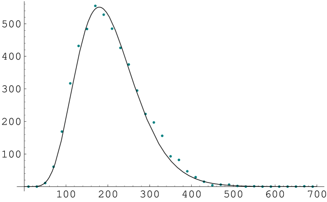
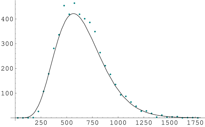
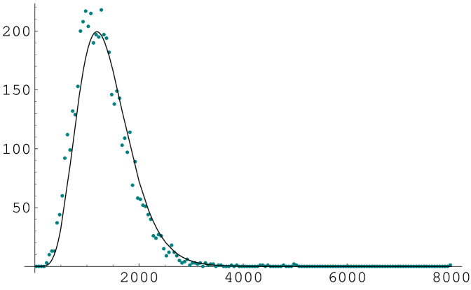
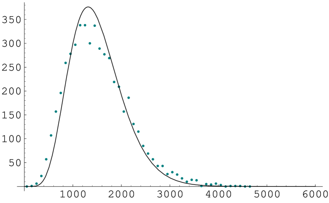
The distribution of nucleation times for 5000 bubbles is shown in Fig. 8 at successively lower temperatures. We see that the distribution is not symmetric; it rises quickly and there is a long tail, which is especially pronounced at low temperatures. From these distributions one has to extract nucleation times. We propose that the asymmetric distribution of times should be used as a whole. Namely, we seek an appropriate function to fit the entire distribution of data at each temperature and asymmetry parameter choice.¶¶¶Based on remarks in the literature [10][11] one might expect that the distribution of nucleation times would be exponential. Our results do not show this behavior. Unfortunately, the details of the initial field configuration and the actual distributions of nucleation times are not shown in these references. In the only paper we know of that does show a nucleation time distribution, for a limited statistics sample in a dimensional model, the shape is in qualitative agreement with ours [29]. These authors report exponential fits to the tails of their distributions. This procedure does not give the correct value for the nucleation time because the region of the distribution that is fit is not at long enough times to be in the true exponential tail. We develop this point further in the work below. We observe that the distributions rises to their maxima relatively quickly compared to the time over which the tail of the distribution persists. We guess that a power law function of time will fit this part of the distribution. At long times, a damping function that “overpowers a power law” is the falling exponential. The simplest function that has both of the above properties and has, at least naively, an appropriate interpretation in our problem, is the classic “waiting time” form [30]
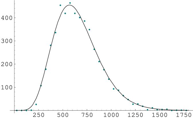
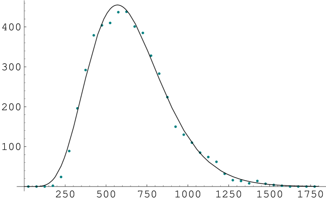
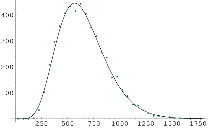
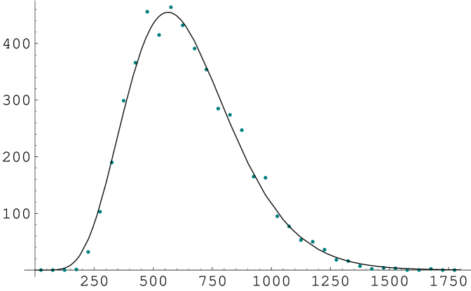
| (15) |
where is the bin size of the histograms. The parameter is what we use for the nucleation time. Both and were obtained from fits to the distributions. The normalization, , can be obtained from the requirement that the integral of Eq. 15 gives the number of bubbles that were used to make the histogram. Fig. 9 shows the least squares fit to this function using a typical additive noise case and Fig. 10 shows the fit for a multiplicative noise case. Figs. 11 and 12 show two more fits with different parameters. These fits were made by setting . From the normalization described above, we checked that this value is approximately correct in all cases. For the same parameters in the models, and at the same temperature, the nucleation times with multiplicative noise is always longer than that for the additive noise case. We emphasize that casting the equations of motion into dimensionless form, detailed in Appendix B, makes direct comparison between the models possible.
B Time vs
At finite temperature the nucleation rate per unit length, in the semi-classical approximation, is given by
| (16) |
where is the Euclidean action corresponding to the bounce solution of the equation of motion and is the temperature. A simple manipulation of this equation gives
| (17) |
where is the length of the lattice. We extracted the nucleation times from the fits as described above and looked at the effects of temperature on nucleation times. To study the fluctuations in the parameters in the fits we generated several data sets for a single set of parameters. We found little variation in the parameters among runs. The tables in Appendix C show a set of fit parameters from different runs. The fluctuations in the parameters and are small, being less that two percent of the central value. The value of is especially stable from one run to another. We emphasize that, when normalized to 1, the average of the fit function is . This should agree with the average of the data; within (small) errors, it does in every case.
We also looked at the fluctuations in the fits at a lower temperature and found that all the fluctuations in the parameters were within five percent of the central value. In fact most were within two percent, with showing smaller variation than , as in the examples shown in the tables in Appendix C.
Using a global error estimate of five percent in the parameter to cover all of the cases we studied, we fitted straight lines to the data plots of nucleation times vs inverse temperature. We show the results for the additive model in Fig. 13. The confidence levels of the fits are , and for and respectively. In Fig. 14. we show the corresponding result for the multiplicative noise model. The confidence levels of the fits are , and for and respectively. Both plots show strong evidence that the relationship between and is linear, reproducing the semiclassical description of the finite temperature quantum system, Eqn. 16.
We see that for both additive and multiplicative noise, the larger values of the asymmetry parameter drive nucleation at a faster rate. This is in agreement with nucleation theory: the action for the bounce, which appears in the exponential of the decay rate, is inversely proportional to the energy difference between the true and false vacua. The plots also show that for a given asymmetry parameter the nucleation time is shorter at higher temperatures as one would expect. As mentioned above, the plots also indicate the linear relationship between and . The new twist is that is extracted by our analysis from the full distribution as a “waiting time”. For long enough times, the waiting time distribution, Eq. 16, has an exponential tail with decay constant . But this is in the time regime , far beyond the point where we run out of simulated events. It would take enormous statistics to probe this regime.
V Discussion and Conclusion
We have studied false vacuum decay in dimensions using Langevin equations on a lattice. We looked at cases where the stochastic term in the equation was in the form of additive noise, previously studied in [10] in , and in the form of the theoretically motivated multiplicative noise case[14]. The cosmological applications of multiplicative noise have been discussed in[28]. In past work [10][11][29] decay times were fit by exponential distributions. We found distributions of nucleation times that were not exponential, as described above. We found that a , or waiting times, fit with effective multiple incidence of about 6, gives a good description of the whole distribution of nucleation times for every case studied. In principle, the tail of the fitting function, Eq. 16, is an exponential with decay time . In practice, the time must satisfy , which far beyond the end of our statistics, even with bubble samples. At shorter times, well past the peak of the distribution but where data is still sufficient in the falling tail, we can find reasonable, approximate exponential fits to the data. However, these fits to the exponential tails do not give the same nucleation times as the distribution, in fact the tails underestimate the nucleation times. Fitting the tails of the distribution also requires one to discard most of the data and hence potential valuable information on the dynamics of nucleation. We found that for both the additive noise and multiplicative noise Langevin models, the semiclassical relationship between nucleation time and temperature is reproduced in the range of parameters studied. For the same set of parameters the multiplicative noise equations give nucleation times that are longer than in the additive case by factors of three or more. To see why this might be so, note that the location of the barrier of the potential, and consequently its stable minimum, are at scaled field values significantly greater than one. So apparently the quadratic field dependence of the viscosity term in the multiplicative case significantly inhibits the thermal hopping process, more than compensating for the enhancement from the linear field dependence of the driving term. We tested this idea by varying the value the field had to attain for a bubble to be declared formed. We expect that the fractional increase in nucleation time as the field value increases should be greater in the multiplicative noise case than in the additive. We looked at three different field value requirements, , and . Tables I and II show that for the same increase in the field value criterion, the nucleation time increases by about in the additive noise model and in the multiplicative noise model. While this is not a proof of our conjecture, the trend demonstrates the importance of the field dependent viscosity in slowing down the nucleation rate.
The distribution which fits the data is the waiting time distribution for a fixed number of events that obey Poisson statistics. The fit parameter is fairly constant throughout the range of input parameters studied, and this points to some quasi-universal feature in the models. The observation that it is of the order of the number of lattice sites, 5, that determines our bubble formation criterion, which is consistent with the field correlation of the initial configuration, may be a clue to the interpretation of the insensitivity of the value of a to the choice of model and of the input parameters for a given model. The full interpretation of the successful application of the distribution to this problem and the significance of the approximate universality of the parameter are currently under study.
VI Appendix A
The fluctuation Dissipation Theorem
The fluctuation-dissipation theorem[24][25], as the name implies, relates the stochastic fluctuations of a system to its dissipative or irreversible properties. As described earlier its application ranges from classical phenomena like Brownian motion to the far more complicated case of a scalar field coupled to a thermal bath. For a general discussion see [31]. In numerical studies like the one reported here, the Langevin equation on its own does not completely describe the coupling of the field to the thermal bath. The fluctuation-dissipation relation, Eqn. 8, is used to connect the stochastic and dissipation terms and hence ensure a realistic simulation if the thermal system. The delta function correlations are implemented numerically by sampling the distribution of fluctuations at each lattice space site and at each time step in propagating the solution of the equation of motion. The exact form of the noise distribution and, in particular, its dependence on the viscosity parameter is important because from this we obtain the correct numerical value of temperature. We describe here in some detail our implementation of the fluctuation dissipation theorem and the noise distribution we sampled in the study.
The probability distribution of the noise is assumed to be Gaussian of the form,
| (18) |
For convenience define and . Then,
| (19) |
Introduce a source for the noise, , in the exponent.
| (21) | |||||
| (23) | |||||
Now re-define to be .
Then,
| (24) |
Therefore,
| (26) | |||||
| (27) | |||||
| (28) |
In the limit we get, after taking the next functional derivative,
| (29) |
VII Appendix B
Re-Scaling The equations of Motion
The parameters and have different units in the additive and multiplicative noise equations of motion. To compare the results of our numerical study we rescale the equations of motion so that all quantities appearing in them are dimensionless.
Consider the potential,
| (30) |
appears in the Hamiltonian density, .
| (31) |
The Hamiltionian, , which has the dimension of energy is obtained from as,
| (32) |
therefore has dimension of . From the term in we get where means “dimension of”. We also have the following;
| (33) | |||||
| (34) | |||||
| (35) | |||||
| (36) | |||||
| (37) |
The subscript refers to additive noise. For the multiplicative noise case and have the dimensions,
| (39) | |||||
| (40) |
We now rescale the field and parameters appearing in the equation of motion. For the purpose of discussion let be the value of the field in the true vacuum.∥∥∥It can also be chosen to be the value that the field takes at the top of the barrier of the potential or the value of the field at a zero of the potential. When the thin wall approximation is not applicable the field value at the escape point at the right of the barrier is the more important quantity. For the additive noise case we have,
| (41) |
We now make the following definitions,
| (42) | |||||
| (43) | |||||
| (44) | |||||
| (45) | |||||
| (46) | |||||
| (47) | |||||
| (48) | |||||
| (49) |
where follows from the fluctuation-dissipation relation, Eqn. 8. The rescaled equation of motion is,
| (50) |
We rescale the multiplicative noise case in a similar manner but the dimensionless viscosity and noise parameters are,
| (51) |
and
| (52) |
The dimensionless equation of motion is then
| (53) |
In terms of the original parameters, the pre-scaled has the dimension of energy but it is dimensionless after re-scaling. The key point is that the parameters , and in the scalar potential can be used to rescale both equations to dimensionless forms. We have used and to illustrate the rescaling but other quantities of the same dimensions can be used as noted. All quantitive work is done with Eqns. 50 and 53, so the values assigned to , determine the value of in the true vacuum in each case. With this understanding, the tilde notation is not used in the text when referring to results from the rescaled equations. Now that the parameters in both equations of motion are dimensionless, we can make direct comparisons of the two models.
VIII Appendix C
Example Data and Fits Used to Determine Fluctuations in and
ACKNOWLEDGMENTS
Conversations and suggestions from Ruslan Davidchack, Brian Laird, John Ralston, and Krzysztof Kuczera at various stages of this work were of great value. We thank Hume Feldman for numerous discussions on his work in this field and for critical comments on some of our early results. We thank Salman Habib for bringing to our attention his earlier work on multiplicative noise. This work was supported in part by U.S. Department of Energy grant number DE-FG03-98ER41079. Facilities of the Kansas Institute for Theoretical and Computational Science and especially the Kansas Center for Advanced Scientific Computing were essential for this work.
REFERENCES
- [1] J. S. Langer, Ann. Phys. 41 108 (1967); 54 258 (1969).
- [2] T. D. Lee and G. C. Wick, Phys. Rev. D9 , 2291, (1974).
-
[3]
Ya. B. Zel’dovich, I. Yu. Kobzarev, and L. B. Okun
Zh. Eksp. Teor. Fiz. 67, 3 (1974) [Sov. Phys.-JETP Vol. 40, No1, 1 (1975)]. -
[4]
M. B. Voloshin, I. Yu. Kobzarev, and L. B. Okun,
Yad. Fiz. 20, 1229 (1974) [Sov. J. Nucl. Phys.Vol.20, No 6, 644 (1975)]. - [5] A. H. Guth, Phys. Rev. D23, 347 (1981).
- [6] S. Coleman, Phys. Rev. D15 , 2929, (1977).
- [7] C. Callan and S. Coleman, Phys. Rev. D16, 1762, (1977).
- [8] A. D. Linde, Nucl. Phys. B216, 421, (1983).
- [9] O.T. Valls and G.F. Mazenko, Phys. Rev. B42, 6614 (1990).
- [10] M. Alford, H. Feldman, and M. Gleiser, Phys. Rev. D47, 2168, (1993).
- [11] M. Alford and M. Gleiser, Phys. Rev. D48, 2838 (1993).
- [12] R. M. Haas, Phys. Rev. D57, 7422 (1998).
- [13] M. Morikawa, Phys. Rev. D33, 3607 (1986).
- [14] M. Gleiser and R. Ramos, Phys. Rev. D50, 2441 (1994).
- [15] C. Greiner and B. Müller, Phys. Rev. D55, 1026 (1997).
- [16] S. Alamoudi, D. G. Barci, D. Boyanovsky, C. A. A. de Carvalho, E. S. Fraga, S. E. Joras and F. I. Takakura, Phys. Rev. D60, 125003 (1999); Da-Shin Lee and D. Boyanovsky, Nucl. Phys. B406, 631 (1993).
- [17] F. J. Alexander, S. Habib, and A. Kovner, Phys. Rev. E48, 4284 (1993)
- [18] G. Parisi, Statistical Field Theory (Addison Wesley Publishing Company, 1988). This reference gives a helpful discussion in the field theory context.
- [19] A. M. Polyakov, Nucl. Phys. B120, 429 (1977).
- [20] R.Rajaraman, Solitons and Instantons (North Holland Publishing Co.,1982).
- [21] S. Coleman, V. Glaser, and A. Martin, Commun. Math. Phys. 58, 211 (1978).
- [22] T. Matsubara, Progress of Theoretical Physics, 14, 351(1955).
- [23] T. Koide, M. Maruyama and F. Takagi, hep-ph/0102272. The results obtained by these authors, using a different technique, differ in some respects from those of [14][15] when applied to quantum field theory.
- [24] R. Kubo, J. Phys. Soc. Jap. 12, 570 (1957).
- [25] S. Chandrasekhar, Rev. Mod. Phys. 15, 1 (1943).
- [26] H. Press, S. Teukolsky, W. Vetterling, and B. Flannery, Numerical Recipes in Fortran (Cambridge University Press,1992).
- [27] N. D. Antunes and L. M. A. Bettencourt, Phys. Rev. D55, 925 (1997).
- [28] S. Habib and H. E. Kandrup, Phys. Rev. D46, 5303 (1992).
- [29] S. Borsanyi, A. Patkos, J. Polonyi, and Z. Szep, Phys. Rev. D62, 085013 (2000).
- [30] E. Parzen, Modern Probability Theory and its Application (John Wiley and Sons, Inc., 1960).
- [31] H. B. Callen and T. A. Welton, Phys. Rev. 83, 34 (1951)


a (b)


() ()


() ()


() ()


() ()


(a) (b)


(c) (d)


|
|
|
|
|
|
|
|