An Exact Solution to a Three Dimensional Ising Model and Dimensional Reductions

Abstract

A high temperature expansion is employed to map some complex anisotropic nonhermitian three and four dimensional Ising models with algebraic long range interactions into a solvable two dimensional variant. We also address the dimensional reductions for anisotropic two dimensional XY and other models. For the latter and related systems it is possible to have an effective reduction in the dimension without the need of compactifying some dimensions. Some solutions are presented. This framework further allows for some very simple general observations. It will be seen that the absence of a “phase interference” effect plays an important role in high dimensional problems. A very forbidding purely algebraic recursive series solution to the three dimensional nearest neighbor Ising model will be given. In the aftermath, the full-blown three dimensional nearest neighbor Ising model is exactly mapped onto a single spin 1/2 particle with nontrivial dynamics. All this allows for a formal high dimensional Bosonization.

]

I Introduction

In this article, a high temperature expansion is employed to examine mappings between problems of various dimensionality. By these reductions we will exactly solve an anisotropic two dimensional XY and some other models. It will be seen that the absence of a “phase interference” effect plays an important role in high dimensional problems; this observation will allow us to examine various high dimensional models by averaging over newly constructed one dimensional systems. In turn, this averaging process will formally allow us to effectively bosonize high dimensional theories.

In section II, I am going to start off by discussing a momentum space high temperature expansion. Next, by analytically continuing the momenta and making them complex (section III) , quaternion (section IV), and of a general matrix form we will be able to exactly solve a variety of two, three, and four dimensional Ising and $O(n)$ models. Many of these models are artificial and correspond to non hermitian anisotropic long range interactions. Some of the resulting models will be short ranged and of real hermitian form. We will exactly solve some special simple two dimensional anisotropic XY models

We will then extend these techniques to the quantum case and discuss “2+1 dimensional Bethe Ansatz” solutions in section(V) where we will also solve a special two dimensional anisotropic XY model.

After solving these models, in subsection(VI A) we will apply the high temperature expansion to reduce the three dimensional nearest neighbor Ising ferromagnet into an illusory formal solvable expression written in a determinant notation. In this method, the high temperature coefficient to each order is arrived at by looking a single linear relation originating from a matrix of (super exponentially) increasing order.

In subsection(VI B), we will map the nearest neighbor $d$ dimensional Ising models to an ensemble average over a spin chain with long ranged “Coulomb” like interaction. In this scenario each spin is effectively composed of $d$ constituent charges each generating its own shifted “Coulomb” like field. This in turn will enable us to map the $d$ dimensional Ising model onto a a single spin 1/2 quantum particle in 0+1 dimensions. We will apply the dimensional reduction techniques to quantum spin problems where an effective one dimensional fermion problem will result.

In section(VII), I will discuss a “permutational” symmetry present in the $O(n\rightarrow\infty)$ models but violated to ${\cal{O}}(\beta^{4})$ in finite $n$ problem. This will again allow us to map any large $n$ problem onto a one dimensional system but this time without the need of averaging.

One of the main motifs of this article is the absence or presence of “momentum interference” effects in high and low dimensional problems respectively.

II A momentum space high temperature expansion

We will for the most part examine simple classical spin models of the type

$$H=\frac{1}{2}\sum_{\vec{x},\vec{y}}\hat{V}(\vec{x},\vec{y})[\vec{S}(\vec{x})\cdot\vec{S}(\vec{y})].$$ (1)

Here, the sites $\vec{x}$ and $\vec{y}$ lie on a (generally hypercubic) lattice of size $N$. The spins $\{S(\vec{x})\}$ are normalized and have $n$ components. The kernel $\hat{V}(\vec{x},\vec{y})$ is translation invariant. The $n=1$ case simply corresponds to the Ising model.

Later on, when we will discuss quaternion models we will replace the scalar product by a slightly more complicated product.

The Hamiltonian in the (non-symmetrical) Fourier basis is diagonal ($f(\vec{k})=\sum_{\vec{x}}F(\vec{x})e^{-i\vec{k}\cdot\vec{x}};$

$~{}F(\vec{x})=\frac{1}{N}\sum_{\vec{k}}f(\vec{k})e^{i\vec{k}\cdot\vec{x}}$) and reads

$$H=\frac{1}{2N}\sum_{\vec{k}}\hat{v}(\vec{k})|\vec{S}(\vec{k})|^{2}$$ (2)

where $\hat{v}(\vec{k})$ and $\vec{S}(\vec{k})$ are the Fourier transforms of $\hat{V}(\vec{x})$ and $\vec{S}(\vec{x})$ respectively.

For simplicity, we will set the lattice constant to unity- i.e. on a hypercubic lattice (of side $L$) with periodic boundary conditions (which we will assume throughout) the wave-vector components $k_{l}=\frac{2\pi r_{l}}{L}$ where $r_{l}$ is an integer (and the real space coordinates $x_{l}$ are integers).

In the up and coming $V\equiv\beta\hat{V}$. For an invertible $\hat{V}(\vec{x},\vec{y})$, and $0<\beta<\infty$ (via a Hubbard-Stratonovich transformation [4]):

$$Z=Tr\exp\{-\frac{1}{2}\sum_{\vec{x},\vec{y}}V(\vec{x},\vec{y})S(\vec{x})S(\vec{y})\}$$ (3)

$$=\sqrt{\det(-\frac{2}{\pi V})}\int\prod_{\vec{x}}d\eta(\vec{x})\exp[-H\{\eta(\vec{x})\}]$$ (4)

where

$$H[\{\eta(\vec{x})\}]=-\frac{1}{2}\sum_{\vec{x},\vec{y}}\eta(\vec{x})V^{-1}(\vec{x},\vec{y})\eta(\vec{y})$$ (5)

$$-\sum_{\vec{x}}\ln[\cosh\eta(\vec{x})]$$ (6)

and analogously for the $O(n>1)$ model

$$H\{\vec{\eta}(\vec{x})\}=-\frac{1}{2}\sum_{\vec{x},\vec{y}}V^{-1}(\vec{x},\vec{y})\vec{\eta}(\vec{x})\cdot\vec{\eta}(\vec{y})$$ (7)

$$-\sum_{\vec{x}}\ln[~{}\Gamma(n/2)~{}(\frac{2}{|\vec{\eta}(\vec{x})|})^{n/2-1}~{}I_{n/2-1}(|\vec{\eta}(\vec{x})|)~{}]$$ (8)

with $I_{n/2-1}(z)$ a Bessel function.

The $\cosh\eta$ or Bessel terms may be viewed as terms of constraint securing the normalization of $\vec{S}(\vec{x})$ at every site $\vec{x}$.

If a magnetic field $h(\vec{x})$ were applied, the argument of the $cosh$ would be replaced $\cosh(\eta+h)$ with a similar occurrence for the Bessel function appearing for the $O(n>1)$ models.

The $q-$state Potts model can be viewed as a spin model in which the $q$ possible polarizations of the spins lie at the vertices of a $(q-1)$ dimensional tetrahedron- in this manner the scalar product amongst any two non identical spins is $\cos^{-1}(-1/(q-1))$. Employing this representation, the sum $\sum_{\vec{x}}\ln\cosh\eta(\vec{x})$ may be replaced by $\sum_{\vec{x}}\ln\sum_{i=1}^{q}\exp[\vec{S}_{i}\cdot\vec{\eta}]$ where the sum is over the $q$ polarizations of the $(q-1)$ dimensional spin $\vec{S}_{i}$.

The partition function of the Ising spins reads

$$Z=\sqrt{\det(-\frac{2}{\pi V})}\int D\eta e^{-\beta H}$$ (9)

$$=\sqrt{\det(-\frac{2}{\pi V})}\int\prod_{\vec{x}}d\eta(\vec{x})$$ (10)

$$\exp\Big{[}-\frac{1}{2}\sum_{\vec{x},\vec{y}}\eta(\vec{x})V^{-1}(\vec{x},\vec{y})\eta(\vec{y})\Big{]}$$ (11)

$$\prod_{\vec{x}}\cosh\eta(\vec{x}).$$ (12)

For a translationally invariant interaction $V(\vec{x},\vec{y})=V(\vec{x}-\vec{y})$, this may be written in momentum space

$$Z=\sqrt{\det(-\frac{2}{\pi V})}\int D\eta\exp\Big{[}-\frac{1}{2N}$$ (13)

$$\sum_{\vec{k}}v^{-1}(\vec{k})\eta(\vec{k})\eta(-\vec{k})\Big{]}$$ (14)

$$\prod_{\vec{x}}\sum_{m=0}^{\infty}\frac{\eta^{2m}(\vec{x})}{(2m)!},$$ (15)

where $v(\vec{k})$ is the Fourier transform

$$v(\vec{k})=\sum_{\vec{x}}V(\vec{x}-\vec{y})e^{i\vec{k}\cdot\vec{x}}\equiv\beta\hat{v}(\vec{k}).$$ (16)

where the sum is over all lattice sites $\vec{x}$. Thus the partition function is , trivially,

$$Z={\cal{N}}\sum_{m_{1},...m_{N}}\langle\prod_{i=1}^{N}\frac{1}{(2m_{i})!}\eta^{2m_{i}}(\vec{x}_{i})\rangle_{0}$$ (17)

where $\langle~{}~{}\rangle_{0}$ denotes an average with respect to the unperturbed Gaussian weight

$$\exp\Big{[}-\frac{1}{2N}\sum_{\vec{k}}v^{-1}(\vec{k})\eta(\vec{k})\eta(-\vec{k})\Big{]},$$ (18)

and ${\cal{N}}$ is a normalization constant. Each contraction $\langle\eta(\vec{x})\eta(\vec{y})\rangle$ (or $\langle\eta(\vec{k})\eta(-\vec{k})\rangle$) leads to a factor of $V(\vec{x},\vec{y})=\beta\hat{V}(\vec{x},\vec{y})$ (or to $\beta\hat{v}(\vec{k})/N$ in momentum space). Thus the resultant series is an expansion in the inverse temperature $\beta$. In the up and coming we will focus attention on the momentum space formulation of this series. All the momentum space algebra presented above is only a slight modification to the well known high temperature expansions usually generated by the Hubbard Stratonovich transformation directly applied to the real space representation of the fields $\eta(\vec{x})$ [5, 6]. It is due to the naivete of the author that such a redundant momentum space formulation was rederived in the first place. However, as we will see, in momentum space some properties of the series become much more transparent. To make $V$ invertible and the expansion convergent, we will shift $\hat{v}(\vec{k})$ by a constant

$$\hat{v}(\vec{k})\rightarrow\hat{v}(\vec{k})+A$$ (19)

such that $\hat{v}(\vec{k})$ is strictly positive. In real space such a constant shift amounts to a trivial shift in the on site interaction (or chemical potential)

$$\hat{V}(\vec{x},\vec{y})\rightarrow\hat{V}(\vec{x},\vec{y})+A.\delta_{\vec{x},\vec{y}}$$ (20)

For asymptotically large $|\eta|$ the nontrivial

$$H^{dual}_{1}\equiv\sum_{\vec{x}}\ln|\cosh\eta(\vec{x})|$$ (21)

is linear in $|\eta|$. The Gaussian generating

$$H^{dual}_{0}=\frac{1}{2}\sum_{\vec{x},\vec{y}}\eta(\vec{x})V^{-1}(\vec{x},\vec{y})\eta(\vec{y})$$ (22)

is a positive quadratic form and dominates at large $\eta$. So far all of this has been very general. Now let us consider the $d$ dimensional nearest neighbor Ising model. To avoid carrying minus signs around, we will consider an Ising antiferromagnet whose partition function is, classically, identically equal to that of a ferromagnet. The exchange constant $J$ will be set to unity. The corresponding momentum space kernel

$$\hat{v}(\vec{k})=A+\sum_{l=1}^{d}[e^{ik_{l}}+e^{-ik_{l}}].$$ (23)

As the reader might guess, the uniform shift $A$ only leads to a trivial change in $Z$ (i.e. to a multiplication by the constant $\exp[-\beta AN]$). In the forthcoming we will set $A=0$.

Owing to the relation

$$\int_{-\pi}^{\pi}dk~{}e^{ikN}=2\pi\delta_{N,0}$$ (24)

all loop integrals are trivial. A simple integral is of the type

$$\int_{\sum_{i=1}^{M}\vec{k}_{i}=0}\prod_{i=1}^{M}\frac{d^{d}k_{i}}{(2\pi)^{d}}\prod_{i}v^{n}(\vec{k}_{i})$$ (25)

$$=\sum_{n=\sum_{l=1}^{d}(\gamma_{l}+\delta_{l})}[\frac{n!}{\prod_{l=1}^{d}\gamma_{l}!\delta_{l}!}]^{M}$$ (26)

(when $n=1$ this integral is $2d$ etc). A related integral reads

$$\int\frac{d^{d}k}{(2\pi)^{d}}\prod_{\sum_{i=1}^{M}\vec{k}_{i}=0}~{}~{}[v(\vec{k}_{i})]^{n_{i}}$$ (27)

$$=\sum_{\gamma_{l}^{i}-\delta_{l}^{i}=m_{i}^{l},~{}\sum_{i=1}^{M}m_{i}^{l}=0,~{}\sum_{l=1}^{d}\gamma_{l}^{i}+\delta_{l}^{i}=n_{i}}\prod_{i=1}^{M}[\frac{n_{i}!}{\prod_{l=1}^{d}\gamma_{l}^{i}!\delta_{l}^{i}!}]$$ (28)

where in the last sum $m_{j<n}^{l}\neq m_{i<M}^{l}=-m_{i=M}^{l}$ etc. Note that the high temperature expansion becomes simpler if instead of symmetrizing the interaction (each bond being counted twice- once by each of the two interacting spins) one considers

$$\hat{v}(\vec{k})=2\sum_{l=1}^{d}\exp[ik_{l}].$$ (29)

Here each spin interacts with only $d$ (and not $2d$) of its neighbors separated from it by one positive distance along the d axes $\hat{e}_{l=1}^{d}$. The factor of 2 originates as each bond is now counted only once and therefore the corresponding bond strength is doubled. The partition function Z is trivially unchanged.

In the most general diagram the propagator momenta $\{\vec{q}_{a}\}$ ($1\leq a\leq$ number of propogators) are linear combinations of the independent loop momenta $\{\vec{k}_{b}\}_{b=1}^{\mbox{loops}}$

$$\vec{q}_{a}=M_{ab}\vec{k}_{b}.$$ (30)

Symmetry factors aside, the value of a given diagram reads

$$\int\prod_{b}\frac{d^{d}k_{b}}{(2\pi)^{d}}\prod_{a}v(\Sigma M_{ab}k_{b})$$ (31)

$$=\int\prod_{b}\frac{d^{d}k_{b}}{(2\pi)^{d}}\prod_{a}(2\beta)\Sigma_{l=1}^{d}\exp[i\Sigma_{b}M_{ab}k_{b}^{l}]$$ (32)

$$=(2\beta)^{\mbox{propagators}}$$ (33)

$$\times\prod_{b=1}^{\mbox{loops}}\Big{(}\int\frac{d^{d}k_{b}}{(2\pi)^{d}}\Sigma_{l=1}^{d}\exp[i\sum_{a,b}M_{ab}k_{b}^{l}]\Big{)}$$ (34)

- i.e. upon expansion of the outer sum, just a product of individual loop integrals of the type encountered in Eqn.(24) for each $k^{l}_{b}$.

The latter integral in $d=1$ reads

$$I=\prod_{b=1}^{\mbox{loops}}\delta(\Sigma_{a=1}^{\mbox{propagators}}M_{ab},0)$$ (35)

The situation in $d>1$ becomes far richer. One may partition the integral into all possible subproducts of momenta corresponding to different spatial components $l$ satisfying the delta function constraints. In a given diagram not all propagators need to correspond to the same spatial component $k^{l}$. The combinatorics of “in how many ways loops may be chosen to satisfy the latter delta function constraints?” boils down to the standard counting of closed loops in real space.

Some simple technical details of lattice perturbation theory vis a vis the standard continuum theories are presented in [10].

III An exact solution to a three dimensional Ising model

Theorem:

If the spin spin interaction on a cubic lattice has a non hermitian kernel of the form

$$\hat{V}(x_{1},x_{2},x_{3})=-\delta_{x_{2},0}\delta_{x_{3},0}(\delta_{x_{1},1}+\delta_{x_{1},-1})$$ (36)

$$-\frac{1}{\pi}(-1)^{x_{3}}\frac{\sinh\pi\lambda}{\lambda^{2}+x_{3}^{2}}\delta_{x_{1},0}\Big{[}\lambda(\delta_{x_{2},1}+\delta_{x_{2},-1})$$ (37)

$$+ix_{3}(\delta_{x_{2},1}-\delta_{x_{2},-1})]\Big{]}$$ (38)

then, for all real $\lambda$, the Helmholtz free energy per spin $a(h=0,T)$ is

$$\beta f=-\ln(2\cosh 2\beta)-$$ (39)

$$\frac{1}{2\pi}\int_{0}^{\pi}d\phi\ln\frac{1}{2}(1+\sqrt{1-\kappa^{2}\sin^{2}\phi})$$ (40)

where

$$\kappa\equiv\frac{2\sinh 2\beta}{\cosh^{2}2\beta}$$ (41)

and the internal energy per spin

$$u=-\coth 2\beta\Big{[}1+\frac{2}{\pi}\kappa^{\prime}K_{1}(\kappa)\Big{]}$$ (42)

where $K_{1}(\kappa)$ is a complete integral of the first kind

$$K_{1}(\kappa)\equiv\int_{0}^{\pi/2}\frac{d\phi}{\sqrt{1-\kappa^{2}\sin^{2}\phi}}$$ (43)

and

$$\kappa^{\prime}\equiv 2\tanh^{2}(2\beta)-1.$$ (44)

The proof is quite simple. The expressions presented are the corresponding intensive quantities for the two dimensional nearest neighbor Ising model[1].

Let us start by writing down the diagrammatic expansion for the two dimensional Ising model and set

$$\hat{v}(q_{1},q_{2})\rightarrow\hat{v}(q_{1},q_{2}+i\lambda q_{3})$$ (45)

in all integrals. This effects

$$\int_{-\pi}^{\pi}dk_{2}e^{ik_{2}N^{loop}}\rightarrow\int_{-\pi}^{\pi}dk_{2}e^{ik_{2}N^{loop}}\int_{-\pi}^{\pi}dk_{3}e^{-\lambda k_{3}N^{loop}}$$ (46)

for all individual loop integrals. The integrals are nonvanishing only if $\{N_{b}=0\}$ for all loops $b$. When $N^{loop}=0$ for a given loop the second ($k_{3}$ integration) leads to a trivial multiplicative constant (by one). In the original summation

$$\sum_{\vec{k}_{b}}\rightarrow\frac{L^{d}}{(2\pi)^{d}}\int_{-\pi}^{\pi}...\int_{-\pi}^{\pi}d^{d}k_{b}$$ (47)

and thus an additional factor of $L$ is introduced for each independent connected diagram. Thus the free energy per unit volume for a system with the momentum space kernel $\hat{v}(k_{1},k_{2}+i\lambda k_{3})$ is the same as for the two dimensional nearest neighbor ferromagnet with the kernel $\hat{v}(k_{1},k_{2})$. Fourier transforming $\hat{v}(k_{1},k_{2}+i\lambda k_{3})$ and symmetrizing $[V(\vec{x})+V(-\vec{x})]/2\rightarrow V(\vec{x})$ one finds the complex real space kernel $\hat{V}(x_{1},x_{2},x_{3})$ presented above [11] Q.E.D.

Corollary

For the more general

$$\hat{V}(x_{1},x_{2},x_{3})=-\delta_{x_{2},0}\delta_{x_{3},0}(\delta_{x_{1},1}+\delta_{x_{1},-1})$$ (48)

$$-{\cal{J}}\delta_{x_{1},0}\Big{[}\frac{(-1)^{x_{3}}}{\lambda^{2}+x_{3}^{2}}\Big{]}\{(\delta_{x_{2},1}+\delta_{x_{2},-1})$$ (49)

$$+i(\delta_{x_{2},-1}-\delta_{x_{2},1})\frac{x_{3}}{\lambda}\}$$ (50)

we may define

$$r\equiv\frac{\pi{\cal{J}}}{2\lambda~{}\sinh\pi\lambda}$$ (51)

to write the free energy as the free energy of an anisotropic two dimensional nearest neighbor ferromagnet with the kernel

$$\hat{V}(x_{1},x_{2})=-\delta_{x_{2},0}(\delta_{x_{1},1}+\delta_{x_{1},-1}$$ (52)

$$-r\delta_{x_{1},0}(\delta_{x_{2},1}+\delta_{x_{2},-1})$$ (53)

i.e. a nearest neighbor Ising ferromagnet having the ratio of the exchange constants along the $x_{1}$ and $x_{2}$ axes equal to $r=J_{2}/J_{1}$ (throughout we set $J_{1}$ to unity). Introducing

$$u\equiv\frac{1}{\sinh 2\beta\sinh 2\beta r}$$ (54)

and defining

$$F(\theta)\equiv\ln\{2[\cosh 2\beta\cosh 2\beta r$$ (55)

$$+u^{-1}(1-2u\cos\theta+u^{2})^{1/2}]\},$$ (56)

we may write the free energy density as

$$\beta f=-\frac{1}{2\pi}\int_{0}^{\pi}F(\theta).$$ (57)

Note that the same result applies for the “ferromagnetic”

$$\hat{V}(x_{1},x_{2},x_{3})=-\delta_{x_{2},0}\delta_{x_{3},0}(\delta_{x_{1},1}+\delta_{x_{1},-1})$$ (58)

$$-{\cal{J}}\delta_{x_{1},0}\Big{[}\frac{1}{\lambda^{2}+x_{3}^{2}}\Big{]}\{(\delta_{x_{2},1}+\delta_{x_{2},-1})$$ (59)

$$+i(\delta_{x_{2},-1}-\delta_{x_{2},1})\frac{x_{3}}{\lambda}\}.$$ (60)

The proof is simple- the partition function is identically the same if evaluated with the kernel in Eqn.(60) instead of that in Eqn.(50) if the spins are flipped

$$S(\vec{x})\rightarrow(-1)^{x_{3}}S(\vec{x}).$$ (61)

What about correlation functions? The equivalence of the partition functions $Z[\beta,h(x_{1},x_{2})]$ implies that in the planar directions the correlations are the same as for two dimensional ferromagnet.

Changing the single momentum coordinate

$$v(k_{1},k_{2})\rightarrow v(k_{1},k_{2}+i\lambda k_{3})$$ (62)

effects

$$G(k_{1},k_{2})\rightarrow G(k_{1},k_{2}+i\lambda k_{3})$$ (63)

in the momentum space correlation function. The algebra is identically the same.

The connected spatial correlations (for $T\neq T_{c}$) are exponentially damped along the $x_{2}$ axis as they are in the usual two dimensional nearest neighbor ferromagnet (see [2, 3] for the two dimensional correlation function).

Of course, all of this can also be extended to one-dimensional like spin systems.

The two dimensional spin-spin kernel

$$\hat{V}(x_{1},x_{2})=-\frac{1}{\pi}(-1)^{x_{2}}\frac{\sinh\pi\lambda}{\lambda^{2}+x_{2}^{2}}\delta_{x_{1},0}\Big{[}\lambda(\delta_{x_{2},1}+\delta_{x_{2},-1})$$ (64)

$$+ix_{2}(\delta_{x_{2},1}-\delta_{x_{2},-1})]\Big{]}$$ (65)

leads to one dimensional behavior with oscillatory oscillations along the $x_{2}$. More precisely, the momentum space correlator for any $O(n)$ system in one dimension reads

$$G(k)=\frac{e^{r}}{e^{r}-e^{ik}}+\frac{1}{e^{ik+r}-1}.$$ (66)

For the Ising ($n=1$) system $r\equiv-[\ln\tanh\beta]$. One may set $k=k_{1}+i\lambda k_{2}$ and compute the inverse Fourier transform. The correlations along $x_{2}$ are oscillatory with temperature dependent wavevectors. In other words, the effective correlation length along $x_{2}$ is infinite.

If the two dimensional spin-spin interactions in Eqn.(65) are augmented by an additional on-site magnetic field $h$ then the two dimensional partition function reads

$$Z=\lambda_{+}^{N}+\lambda_{-}^{N}$$ (67)

where, as usual,

$$\lambda_{\pm}=e^{\beta}\cosh\beta h\pm\sqrt{e^{2\beta}\sinh^{2}\beta h+e^{-2\beta}}.$$ (68)

That “complexifying” the coordinates should not change the physics is intuitively obvious: if one shifts $k_{1}\rightarrow k_{1}+\lambda k_{2}\equiv k^{\prime}_{1}$ with real $\lambda$ in the one dimensional $\hat{v}(k_{1})$ then the resulting kernel is $\hat{v}(k^{\prime}_{1})$ plainly describes a stack on chains parallel to $(1,\lambda)$; the spins interact along the chain direction yet the chains do not interact amongst themselves. The free energy density should be identically equal to that of a one dimensional system- no possible dependence on $\lambda$ can occur. All that we have done in the above is allow $\lambda$ to become complex.

In

$$\hat{v}(k_{1},k_{2})\rightarrow\hat{v}(k_{1},k_{2}+\lambda k_{3})$$ (69)

the correlation functions along a direction orthogonal to the direction $(1,\lambda)$ in the $(x_{2},x_{3})$ plane vanish. If $\lambda$ is complex then there are no correlations along an orthogonal direction in the “complex” space.

Formally, all this stems from the trivial fact that the measure $dk_{1}dk_{2}=const(dkdk^{*})$, whereas $\hat{v}(k)$ depends only on the single complex coordinate $k$.

Other trivial generalizations are possible. For example, we may make both $k_{1}$ and $k_{2}$ complex in $\hat{v}(k_{1},k_{2})$ to generate a four dimensional spin kernel

$$\hat{V}(x_{1},x_{2}.x_{3},x_{4})$$ (70)

$$=-\frac{1}{\pi}\Big{(}(-1)^{x_{2}}\frac{\sinh\pi\lambda_{1}}{\lambda_{1}^{2}+x_{2}^{2}}\delta_{x_{1},0}\Big{[}\lambda_{1}(\delta_{x_{2},1}+\delta_{x_{2},-1})$$ (71)

$$+ix_{3}(\delta_{x_{2},1}-\delta_{x_{2},-1})]\Big{]}$$ (72)

$$+(-1)^{x_{4}}\frac{\sinh\pi\lambda_{2}}{\lambda_{2}^{2}+x_{4}^{2}}\delta_{x_{3},0}\Big{[}\lambda_{2}(\delta_{x_{4},1}+\delta_{x_{4},-1})$$ (73)

$$+ix_{4}(\delta_{x_{3},1}-\delta_{x_{3},-1})]\Big{]}\Big{)}$$ (74)

which leads to the canonical (nearest neighbor) two dimensional behavior for arbitrary $\lambda_{1}$ and $\lambda_{2}$.

All of this need not be restricted to cubic lattice models. We may also analytically continue $\hat{v}(\vec{k})$ of the triangular lattice etc.

For the triangular antiferromagnet/ferromagnet

$$v(\vec{k})=\pm 2[\cos k_{1}+\cos(\frac{{k}_{1}}{2}+\frac{\sqrt{3}}{2}k_{2})$$ (75)

$$+\cos(-\frac{k_{1}}{2}+\frac{\sqrt{3}}{2}k_{2})].$$ (76)

Making $k_{2}$ complex leads to interactions on a layered triangular lattice etc.

IV Higher $O(n>1)$ models

The multi-component $O(n>1)$ spin models display a far richer variety of possible higher dimensional extensions.

$\lambda$ need not be only a complex number, it may also be quaternion or correspond to more general set of matrices.

Let us examine the extension to “quaternion” $\vec{k}$ (or with the matrices $i\sigma_{1},i\sigma_{2}$,and $i\sigma_{3}$ (with $\{\sigma_{\alpha}\}$ the Pauli matrices) taking on the role of $i,j$ and $k$). If we were dealing with an $O(2)$ (or XY) model, the same high temperature expansion could be reproduced:

We may envisage a trivial extension to the usual scalar product Hamiltonian

$$H=\frac{1}{2}\sum_{\vec{x},\vec{y}}\hat{V}(\vec{x}-\vec{y})\vec{S}(\vec{x})\cdot\vec{S}(\vec{y})$$ (77)

to one in which the kernel is no longer diagonal in the internal spin indices $\alpha,\beta=1,2$.

$$H=\frac{1}{2}\sum_{\vec{x},\vec{y}}\hat{V}_{\alpha,\beta}(\vec{x}-\vec{y})S_{\alpha}(\vec{x})S_{\beta}(\vec{y}).$$ (78)

The high temperature expansion may be reproduced as before with the kernel $V_{\alpha,\beta}(\vec{x}-\vec{y})$ being generated by each contraction of $\eta_{\alpha}(\vec{x})$ and $\eta_{\beta}(\vec{y})$, or in momentum space $v_{\alpha,\beta}(\vec{k})\delta_{\vec{k}+\vec{k}^{\prime},0}$ is generated by the contraction of $\eta_{\alpha}(\vec{k})$ and $\eta_{\beta}(\vec{k}^{\prime})$.

Let us start off with a nearest neighbor one dimensional XY chain and consider the transformation

$$\exp[ik_{1}]\rightarrow\exp[i(k_{1}+i\lambda_{1}k_{2}\sigma_{1}+i\lambda_{2}k_{3}\sigma_{2}+i\lambda_{3}k_{4}\sigma_{3})]$$ (79)

$$\equiv\exp[ik_{1}-\vec{w}\cdot\vec{\sigma}].$$ (80)

In the argument of the exponential the identity matrix $1$ commutes with $\vec{w}\cdot\vec{\sigma}$ and the exponential may be trivially expanded as

$$\exp[ik_{1}-\vec{w}\cdot\vec{\sigma}]=\exp[ik_{1}]\exp[-\vec{w}\cdot\vec{\sigma}].$$ (81)

Once again in higher dimensions (this time $d=4$) the $k_{1}$ integration will reproduce the familiar

$$\int_{-\pi}^{\pi}dk_{1}\exp[iNk_{1}]=2\pi\delta_{N,0}$$ (82)

for each independent loop momentum $\vec{k}$ and the integration over the remaining $k_{2},k_{3},$ and $k_{4}$ components will simply yield multiplicative constants.

Thus the kernel

$$v(\vec{k})=\exp[ik_{1}-\vec{w}\cdot\vec{\sigma}]+h.c.$$ (83)

will generate a four dimensional XY model which has the partition function of a nearest neighbor one dimensional XY chain. The corresponding real space kernel $\hat{V}(x_{1},x_{2},x_{3},x_{4})$

$$\hat{V}_{\alpha\beta}(x_{1},x_{2},x_{3},x_{4})=\int_{-\pi}^{\pi}...\int_{-\pi}^{\pi}\frac{d^{4}k}{(2\pi)^{4}}\exp[i\vec{k}\cdot\vec{x}]\Big{(}\exp[i(k_{1}$$ (84)

$$+i\lambda_{1}k_{2}\sigma_{1}+i\lambda_{2}k_{3}\sigma_{2}+i\lambda_{3}k_{4}\sigma_{3})]_{\alpha\beta}+h.c.\Big{)}.$$ (85)

In general, this kernel is no longer diagonal in the internal spin coordinates (unless $\vec{w}$ happens to be oriented along $\sigma_{3}$).

$$|\vec{w}|=\sum_{i=2}^{4}\lambda_{i-1}^{2}k_{i}^{2}$$ (86)

$$\hat{w}=(\frac{\lambda_{1}k_{2}}{|\vec{w}|},\frac{\lambda_{2}k_{3}}{|\vec{w}|},\frac{\lambda_{3}k_{4}}{|\vec{w}|})$$ (87)

and

$$\exp[-\vec{\sigma}\cdot\vec{w}]=\cosh(|\vec{w}|)-\sinh(|\vec{w}|)(\vec{\sigma}\cdot\hat{w})$$ (88)

For general $\{\lambda_{i}\}_{i=1}^{3}$ the inverse Fourier transform is nontrivial. The scalar product is replaced by a more complicated product amongst the components. The real space interaction kernel is once again algebraically long ranged along the $x_{2},x_{2}$ and $x_{4}$ axes.

In this manner we may also generate an infinite number of solvable models with a real hermitian kernel. We may state another

Theorem

The hermitian kernel

$$v(\vec{k})=-2\cos(k_{1}+k_{2}\sigma_{3})$$ (89)

leads to the partition function of a one dimensional $O(2)$ chain.

The proof amounts to a reproduction of the calculations given above for the four dimensional $O(2)$ system.

In real space the latter kernel (Eqn.(89)) leads to the $O(2)$ Hamiltonian

$$H=-\sum_{\langle ij\rangle~{}along~{}(1,1)}S_{i}^{(1)}S_{j}^{(1)}-\sum_{\langle ij\rangle~{}along~{}(1,-1)}S_{i}^{(2)}S_{j}^{(2)}$$ (90)

where the $n=1$ (or x component) of the spins interact in the first term and only the y-components of the XY spins appear in the second term; the indices $i$ and $j$ are the two dimensional square lattice coordinates. The first term corresponds to interactions along the $(1,1)$ direction in the plane and the second term corresponds to interactions along the $(1,-1)$ diagonal. The two spin components satisfy $[S_{i}^{(1)}]^{2}+[S_{i}^{(2)}]^{2}=1$- i.e. are normalized at every site $i$. By our mapping, this model trivially has the partition function of a one dimensional nearest neighbor $O(2)$ spin chain.

Similarly, the partition function for the three dimensional kernel $\hat{v}(\vec{k})=-2\cos(k_{1}+k_{2}+k_{3}\sigma_{3})$ is that of a two dimensional nearest neighbor XY model exhibiting Kosterlitz-Thouless like behavior. Here each of two spin components interacts within a different subplane. The coupling between the two spin components due to the normalization constraint apparently plays no role in leaving the system two dimensional.

The reader can easily see how a $d^{\prime}$ dimensional system can be made have an effective dimensionality $1\leq d\leq d^{\prime}$ without the physical need of actual compactification.

Polarization dependent hopping (or “interactions”) akin to those in Eqn.(90) may be of relevance in discussing directed orbital problems in two dimensions.

V Special Two Dimensional Bethe Ansatz solutions

Let us also write the general Hubbard Stratonovich transformation for a Quantum system [8].

Consider a system of fermions with the Hamiltonian

$$H=H_{0}+V$$ (91)

$$H_{0}=\sum_{\alpha\beta}T_{\alpha\beta}a^{\dagger}_{\alpha}a_{\beta}$$ (92)

$$V=\frac{1}{2}\sum_{\alpha\beta\gamma\delta}\langle\alpha\beta|v|\gamma\delta\rangle a^{\dagger}_{\alpha}a^{\dagger}_{\beta}a_{\delta}a_{\gamma}$$ (93)

Following Negele and Orland [8] it is convenient to introduce

$$\hat{\rho}_{\alpha\gamma}=a^{\dagger}_{\alpha}a_{\gamma}$$ (94)

$$K_{\alpha\delta}=T_{\alpha\delta}-\frac{1}{2}\sum_{\beta}v_{\alpha\beta\beta\delta}$$ (95)

where, for our applications, $\vec{\alpha},\vec{\beta},\vec{\gamma},$ and $\vec{\delta}$ are two dimensional position vectors.

For this time independent Hamiltonian

$$\exp[-iH(t_{f}-t_{i})]$$ (96)

$$=\int\prod_{\alpha\beta}D\eta_{\alpha\beta}(t)\exp[\frac{i}{2}\int_{t_{i}}^{t_{f}}dt\eta_{\alpha\beta}(t)v_{\alpha\beta\gamma\delta}\eta_{\gamma\delta}(t)]$$ (97)

$$T\Big{[}\exp[-i\int_{t_{i}}^{t_{f}}dt(K_{\alpha\beta}+\eta_{\gamma\delta}(t)v_{\gamma\alpha\delta\beta})\hat{\rho}_{\alpha\beta}]\Big{]}$$ (98)

Again a momentum space expansion is possible in $\eta_{\alpha\beta}(t)$. If an exact Bethe Ansatz solution is known for nearest neighbor hopping then in some cases it may be extended to two dimensions where the hopping matrix element $K(x_{1},x_{2})$ for separation $\vec{x}=(x_{1},x_{2})=\vec{\alpha}-\vec{\beta}$ attains exactly the same form as the two-dimensional kernel $\hat{V}(x_{1},x_{2})$ just given previously. More generally, the Trotter formula may be employed.

Loosely speaking, if in a fictitious electronic system the hopping matrix element would be the non hermitian

$$K(x_{1},x_{2})=-\frac{1}{\pi}\Big{(}(-1)^{x_{2}}\frac{\sinh\pi\lambda_{1}}{\lambda_{1}^{2}+x_{2}^{2}}\delta_{x_{1},0}$$ (99)

$$\Big{[}\lambda_{1}(\delta_{x_{2},1}+\delta_{x_{2},-1})$$ (100)

$$+ix_{3}(\delta_{x_{2},1}-\delta_{x_{2},-1})\Big{]}\Big{)}$$ (101)

then the system would essentially a one dimensional Luttinger liquid along $x_{1}$. If the kernel would instead decay algebraically along the imaginary time axis the problem would become that of dissipating system.

A hermitian hopping matrix element could also do the trick if we were to consider polarization dependent hopping (or “interactions”) analogous to those in Eqn.(90) and slightly more complicated variants. As noted earlier, such models may be of relevance in discussing directed orbital problems in two dimensions.

For mapping the two dimensional $S=1/2$ Quantum problem of Eqn.(90) onto a nearest neighbor XY chain we find that the free energy density is given by

$$\beta f=-\int_{0}^{1}dx~{}\ln[1+\exp(4\beta\cos(2\pi x))].$$ (102)

VI Phase interference and a mapping onto a single spin problem

We will now map high dimensional ($d>1$) problems onto translationally invariant problems in one dimension.

For the nearest neighbor ferromagnet, the basic idea is to make a comparison between the the kernels

$$\hat{v}_{d}=-2\sum_{l=1}^{d}\cos k_{l}$$ (103)

$$\hat{v}_{1}=-2\sum_{l=1}^{d}\cos c_{l}k_{1}$$ (104)

in $d$ and in one spatial dimensions respectively. Note that the one dimensional problem has, in general, $d$ different harmonics of the single momentum coordinate $k_{1}$. If the coefficients $c_{l}$ are integers equal to $R_{l}$ then the one dimensional problem amounts to a ferromagnetic chain in which each spin interacts with $d$ other spins at distances $\{R_{l}\}_{l=1}^{d}$ away. When evaluating the loop integrals, we will find that the partition function/ free energy deviate from their $d$ dimensional values due to “interference” between the various harmonics in $\hat{v}_{1}(k_{1})$. If all harmonics acted independently then the $d$ dimensional result would be reproduced. The advantages of the form $\hat{v}_{1}$ are obvious. Perhaps the most promising alley is that of “incommensurate dimensional reduction”. By this method, we may examine the d-dimensional problem described by $\hat{v}_{d}$ by a bosonization of the one-dimensional problem of $\hat{v}_{1}$. A solution to the one dimensional problem posed by $\hat{v}_{1}$ followed by an average over the coefficients $\{c_{l}\}$ will immediately lead to the corresponding $d-$ dimensional quantities.

A Commensurate dimensional reduction

Consider a one dimensional ferromagnetic lattice model with a nearest neighbor (or $Range=1$) interaction and a $Range=n$ interaction: $\hat{v}(k_{1})=-2(\cos k_{1}+\cos nk_{1})$. The loop integrals containing terms of the $\cos k_{1}$ origin and terms stemming from $\cos nk_{1}$ are independent to low orders. Mixed terms can survive only to orders $(1/T)^{n+1}$ and higher. The delta function constraints $\sum q_{1}=0$ would generate terms identical to those of the two dimensional nearest neighbor model with $\hat{v}(k_{1},k_{2})=-2(\cos k_{1}+\cos k_{2})$ with the two delta function constraints for the two separate components of the momentum, $\sum q_{1}=0$ and $\sum q_{2}=0$, at every vertex. Thus, in a sense, this system is two dimensional up to $T^{-n}$. Similarly, if a one dimensional chain has interactions of length one lattice constant, $R=n$ and $R=m$ i.e.

$$\hat{v}(k_{1})=-2(\cos k_{1}+\cos nk_{1}+\cos mk_{1})$$ (105)

then this system, as fleshed out by a $1/T$ expansion for the partition function or for the free energy, is three dimensional up to $order~{}=~{}n$ if $m=n^{2}$. (If $m=n+1$ then the triangular ferromagnet is generated). Similar, higher dimensional extensions similarly follow from the lack of commensurability of the cosine arguments (for four dimensions

$$\hat{v}(k_{1})=-2(\cos k_{1}+\cos nk_{1}+\cos mk_{1}+\cos sk_{1})$$ (106)

with $s=n^{2}$ etc.)

The corresponding transfer matrices are trivial to write down. For the three dimensional case:

$$\langle s_{1}...s_{n^{2}}|T|s^{\prime}_{1}...s^{\prime}_{n^{2}}\rangle=\exp[\beta\{\frac{1}{2}(s_{1}s_{2}+...+s_{n^{2}-1}s_{n^{2}})$$ (107)

$$+\frac{1}{2}(s^{\prime}_{1}s^{\prime}_{2}+...+s^{\prime}_{n^{2}-1}s^{\prime}_{n^{2}})$$ (108)

$$+\frac{1}{2}(s_{1}s_{n+1}+s_{2}s_{n+2}+...+s_{n^{2}-n}s_{n^{2}})$$ (109)

$$+\frac{1}{2}(s^{\prime}_{1}s^{\prime}_{n+1}+s^{\prime}_{2}s^{\prime}_{n+2}+...+s^{\prime}_{n^{2}-n}s^{\prime}_{n^{2}})$$ (110)

$$+s_{n^{2}}s^{\prime}_{1}+(s_{n^{2}-n+1}s^{\prime}_{1}+s_{n^{2}-n+2}s^{\prime}_{2}+...+s_{n^{2}}s^{\prime}_{n})$$ (111)

$$+(s_{1}s^{\prime}_{1}+...+s_{n^{2}}s^{\prime}_{n^{2}})\}]$$ (112)

$$\equiv\exp[\beta{\cal{T}}_{ji}].$$ (113)

In higher dimensional generalizations, ${\cal{T}}_{ji}$ will be slightly more nested with the span $n^{2}$ replaced by $n^{d-1}$. In Eqn.(113), the matrix indices $i$ and $j$ are written in binary numerals in terms of the $n^{2}$ spins

$$j=\sum_{\alpha=1}^{n^{2}}(s_{\alpha}+1)2^{\alpha-2}$$ (114)

where $\alpha$ is the one dimensional coordinate along the bra spin indices. By Eqn.(113), ${\cal{T}}_{ji}$ are expressed in terms of a sum over two digit products where the digits are those that appear in the binary (length $n$ spin) representation of the coordinates $j$ and $i$.

As usual, the partition function

$$Z=Tr[T^{N}]=\sum_{i}\lambda_{i}^{N}$$ (115)

where $\{\lambda_{i}\}$ are the eigenvalues of the transfer matrix. In the following $\lambda_{\max}$ will denote the largest eigenvalue.

Note that the transfer matrix eigenvalues correspond to periodic boundary conditions as strictly required: we employed translational invariance to write the partition function expansion in Fourier space. If the boundary conditions are not periodic all this is void.

By the lack of interference effects, the connected diagrams for the free energy are correct to ${\cal{O}}(\beta^{n})$ for interactions with $m=n^{2}$ (Eqn.105). This along with

$$\beta f=\sum_{p}f_{p}\beta^{p}\equiv-\frac{\ln Z}{N}=-\ln\lambda_{\max}$$ (116)

(where the last equality holds in the limit of large system size $N$) and a canonical power expansion having an infinite radius of convergence

$$\lambda_{\max}=\exp[-\sum_{p}f_{p}\beta^{p}]=\sum_{m=0}^{\infty}\Big{(}\frac{1}{m!}(-\sum_{p}f_{p}\beta^{p})^{m}\Big{)}$$ (117)

$$=\sum_{p}b_{p}\beta^{p}$$ (118)

imply that $\lambda_{\max}$ is correct to ${\cal{O}}(\beta^{n})$.

If we already know the lower order coefficients corresponding to ${\cal{O}}(\beta^{p})$ with $p=0,1,2,3,...,(n-1)$ when we consider the $Range=n$ problem. then we may set out to compute is the coefficient of $\beta^{n}$. This will amount to extracting only a single unknown (i.e. the term corresponding to the coefficient of $\beta^{n}$) from a transfer matrix eigenvalue equation, This can be done to the next order etc. recursively. A simple yet very long single linear relation gives the largest transfer matrix eigenvalue to each higher order in the inverse temperature $\beta$.

Explicitly, we can write longhand

$$\det(T-\lambda)=\epsilon_{i_{1}...i_{2^{n^{2}}}}\prod_{j=1}^{2^{n^{2}}}[T_{ji_{j}}(\beta)-\lambda(\beta)\delta_{ji_{j}}]=0$$ (119)

All one has to do is to yank out the ${\cal{O}}(\beta^{n})$ term from the sum over products of $2^{n^{2}}$ terms. If we pull out a power $p_{ji_{j}}$ from each of the elements $[T_{ji_{j}}(\beta)-\lambda(\beta)\delta_{ji_{j}}]$ then those will need to satisfy

$$\sum_{j=1}^{2^{n^{2}}}p_{ji_{j}}=n.$$ (120)

In each element of the transfer matrix, $\exp[\beta{\cal{T}}_{ji}]$, the coefficient of $\beta^{p}$ is trivially ${\cal{T}}_{ji}^{p}/p!$. For each permutation (or “path” of coordinates $(i,j)$ within the matrix) to be summed for the evaluation of the determinant

$$[\sum_{path}{\cal{T}}_{ji_{j}}]^{n}=\sum_{p_{1},p_{2},....,p_{2^{n^{2}}}}\frac{n!}{p_{1}!p_{2}!...p_{2^{n^{2}}}!}\prod_{\sum p_{ji_{j}}=n}{\cal{T}}_{ji_{j}}^{p_{j}}$$ (121)

is exactly the product of the coefficients of $\beta^{p_{ij}}$ such that those lead a net power $\beta^{n}$ (i.e. satisfying Eqn.(120)) from that particular path.

It follows that net contributions stemming from $T_{ji_{j}}(\beta)$ in Eqn.(119) are

$$F^{(n)}\equiv\frac{1}{n!}\sum_{all~{}paths}\epsilon_{path}[\sum_{(ji_{j})~{}in~{}a~{}given~{}path}{\cal{T}}_{ji_{j}}]^{n}$$ (122)

where $\epsilon_{path}$ simply denotes the sign of the given permutation $\{j\}_{j=1}^{2^{n^{2}}}\rightarrow\{i_{j}\}$.

To take into account the products including $\lambda(\beta)$ let us define

$$D^{(n;p)}_{2m}=\frac{1}{(n-p)!}\sum_{all~{}2m~{}paths}$$ (123)

$$\epsilon_{path}[\sum_{(ji_{j})~{}in~{}a~{}given~{}path}^{\prime}{\cal{T}}_{ji_{j}}]^{n-p}$$ (124)

where the summation is over paths going through all possible $(2m)$ given points on the diagonal and $\sum^{\prime}$ denotes a summation over ${\cal{T}}_{ji_{j}}$ in the given paths sans the contributions from the $(2m)$ diagonal points. The determinant paths in $\sum_{all~{}2m~{}paths}$ can pass through more then $(2m)$ diagonal points– it is just that we need to sum over all those that in their pass also traverse all possible sets of $(2m)$ given points on the diagonal and where those points are excluded from the second ${\cal{T}}_{ji_{j}}$ summation.

The $\beta^{n}$ component of Eqn.(119) is

$$F^{(n)}+\sum_{p=0}^{n}\sum_{m=1}^{2^{n^{2}-1}}D_{m}^{(n;p)}\sum_{\sum_{i=1}^{2m}p_{i}=p}b_{p_{1}}...b_{p_{2m}}=0$$ (125)

where $\{b_{p}\}_{p=0}^{n}$ appear in the expansion of the largest eigenvalue (Eqn.(118)).

If the coefficients $\{b_{p}\}_{p=0}^{n-1}$ then Eqn.(125) where $b_{n}$ appears there only linearly gives $b_{n}$ and one may then proceed to look at the eigenvalue equation for the next value of $n$.

In the absence of an external field, for $n=1$ the largest eigenvalue for the $d$ dimensional problem is $\lambda_{+}=2\cosh d\beta$ and other eigenvalue $\lambda_{-}=2\sinh d\beta$. For the three dimensional case setting $m=n^{2}=n=1$ leads to the one dimensional momentum space kernel $\hat{v}(k_{1})=-6\cos k_{1}$ which in real space corresponds to

$$H=-3\sum_{i}S_{i}S_{i+1}.$$ (126)

Of the two eigenvalues only $\lambda_{+}$ has a nonzero $b_{0}$. Knowing the values $b_{0}=2$ and $b_{1}=0$ of the largest eigenvalue we may proceed to find $b_{2}$ from the Eqn.(125) when $n=2$ etc. This, of course, may be extended to systems with magnetic fields.

Setting $b_{0}=2$ in Eqn.(125) we find

$$-b_{n}\sum_{m=1}^{2^{n^{2}-1}}m4^{m}D_{m}^{(n;n)}=$$ (127)

$$F^{(n)}+\sum_{p=0}^{n-1}\sum_{~{}p=p_{1}+p_{2}}b_{p_{1}}b_{p_{2}}D_{1}^{(n;p)}$$ (128)

$$+\sum_{p=0}^{n}\sum_{m=2}^{2^{n^{2}-1}}D_{m}^{(n;p)}\sum_{\sum_{i=1}^{2m}p_{i}=p~{}~{}~{}with~{}p_{i}\neq p}b_{p_{1}}...b_{p_{n}}.$$ (129)

This is the rather explicit recursive relation giving $b_{n}$ once $\{b_{p}\}_{p=0}^{n-1}$ are known. To find out the coefficient of $b_{n}$ let us look at

$$\overline{D}_{s}^{(n;n)}=\sum_{exactly~{}2s~{}diagonal~{}paths}\epsilon_{path},$$ (130)

where the summation admits only those permutations that lead to exactly $2s$ diagonal elements. For the $2^{n^{2}}$ diagonal path in the matrix ${\cal{T}}$: $\epsilon_{path}=1$. For all paths threading $2^{n^{2}-2}$ diagonal sites $\epsilon_{path}=-1$ and the number of such paths is ${2^{n^{2}}\choose 2}$. For the general case the last quantity amounts to

$$\overline{D}_{s}^{(n;n)}=(-1)^{s}{2^{n^{2}}\choose 2s}.$$ (131)

Evaluating, we find

$$D_{m}^{(n;n)}=\sum_{s=m}^{2^{n^{2}-1}}\overline{D}_{s}^{(n;n)}=\frac{(2^{n^{2}})!}{(4m)!(2^{n^{2}}-4m)!}$$ (132)

$$\times F_{pq}[\{1,\frac{m}{2}-2^{n^{2}-1},\frac{1}{2}+\frac{m}{2}-2^{n^{2}-1}\},$$ (133)

$$\{\frac{1}{2}+\frac{m}{2},1+2m\},1]$$ (134)

where $F_{pq}$ is a generalized hypergeometric function.

Insofar as simple geometric visualization is concerned, it is amusing to note, as shown in Fig.(1) for the two dimensional case, that employing the usual high temperature expansion in powers of $\tanh\beta$ one would reach the same conclusion regarding the correctness (up to order $n$) of the partition function evaluated for a width $n$ slab vis a vis the partition function of the two dimensional system. We may look at the a finite thickness $(n$) slab of the two dimensional lattice along which we apply periodic boundary conditions. Let us now draw a string going along one row of length $n$, after which it would jump to the next row, scan it for $n$ sites, jump to the next one, and so on. On the one dimensional laced string, the system is translationally invariant and the interactions are of ranges $R=1,n$. Or, explicitly, by counting the number of closed loops in real space (employing the standard, slightly different, diagrammatic expansion in powers of $\tanh\beta$), we see that the terms in this expansion are also identical up to order $\tanh^{n}\beta$ [12].

A lacing of a two dimensional slab by a one dimensional string, as shown in the figure, is one of the backbones of Density Matrix Renormalization Group Theory when applied to two dimensional problems.

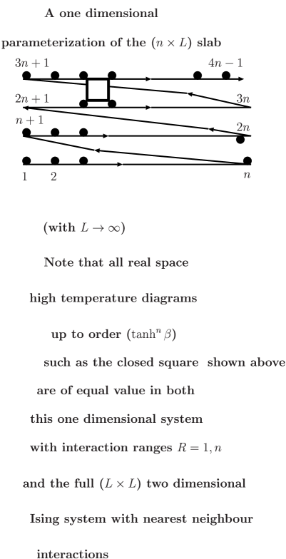
FIG. 1.: Lacing of a “two-dimensional” slab. The width of the slab “$n$” serves as an inverse temperature axis in the following sense- the wider it is, the higher order in $1/T$ that we may advance towards the full two dimensional model. We may get an analogous “three-dimensional” slab with “two imaginary time axis” if we set $m=n^{2}$. The path will then thread $n^{2}$ sites before continuing upward.

B Incommensurate dimensional reduction

Theorem: The one dimensional real space kernel

$$\hat{V}(x_{1})=-2\sum_{l=1}^{d}[(c_{l}+x_{1})\sin\pi(c_{l}-x_{1})$$ (135)

$$+(c_{l}-x_{1})]\sin\pi(x_{1}+c_{l})]$$ (136)

$$\times[(c_{l}-x_{1})(c_{l}+x_{1})]^{-1},$$ (137)

(i.e. a scenario in which each spin is effectively composed of $d$ shifted “Coulombic sources” (more precisely, each spin is composed of $d$ pairs of “charges” generating sinc potentials)) will give rise to the exact $d$ dimensional nearest neighbor partition function and free energies when those quantities are averaged over $\{c_{l}\}_{l=1}^{d}$.

Once again the proof is not too involved. The basic idea is that in momentum space this will give rise to

$$\hat{v}(k_{1})=-2\sum_{l=1}^{d}\cos c_{l}k_{1}$$ (138)

which when averaged over incommensurate $\{c_{l}\}$ will annihilate all phase coherent terms and reproduce the expansion with the $d$ dimensional kernel in Eqn.(23).

Many different measures for $d\mu(c_{l})$ can be chosen. Perhaps the simplest one is

$$\frac{1}{2\Lambda}\int_{-\Lambda}^{\Lambda}dc_{l}$$ (139)

for each of the d coefficients $\{c_{l}\}$.

Performing the $\{c_{l}\}_{l=1}^{d}$ integrations after the loop integrals over $\{k_{a}\}$ we will find that the most general integral is of the form

$$\frac{1}{\Lambda^{d}}\prod_{l=1}^{d}\int_{-\Lambda}^{\Lambda}dc_{l}$$ (140)

$$~{}~{}\Big{[}\prod_{b}\int_{-\pi}^{\pi}\frac{dk_{b}}{2\pi}\prod_{a}\sum_{l=1}^{d}\exp[i\sum_{b}M_{ab}k_{b}c_{l}]~{}\Big{]}$$ (141)

where the index $b$ runs over the various independent loop momenta ($k$ is still merely a scalar for this one dimensional problem). Unless, for a given $k_{b}$ integration, the argument of the exponent is identically zero (i.e. corresponding to a term that would be generated in the d-dimensional nearest neighbor problem) an “interference term” results. However, such a term is down by ${\cal{O}}(\Lambda^{-1})$ by comparison to the “good” noninterference terms that occur in the d-dimensional problem. For each given assignment of $\{c_{l}\}$ along the propagator lines we may perform some coefficient averages over a few of the $\{c_{l}\}$ first and then integrate over the loop momenta and average over the remaining coefficients. For “bad” interference terms, i.e. in those cases in which the argument of the exponential is not identically zero prior to the integration, the canonical integral

$$\frac{1}{2\Lambda}\int_{-\Lambda}^{\Lambda}dc\exp[ick]\rightarrow\frac{\pi\delta(k)}{\Lambda}$$ (142)

will result in the $\Lambda\rightarrow\infty$ limit. When such a delta function is integrated over the momenta in the loop integrals the resulting term is ${\cal{O}}(\Lambda^{-1})$ down by comparison to a noninterference term for which the integral would read

$$\frac{1}{2\Lambda}\int_{-\Lambda}^{\Lambda}dc(1).$$ (143)

In the limit $\Lambda\rightarrow\infty$ such “bad” interference terms will evaporate both in the connected diagrams (for the free energy calculation) as well as for the disconnected diagrams (included in the evaluation of the partition function).

Q.E.D.

Corollary:

For a single spin 1/2 particle with an action

$$S=\int_{0}^{\beta}d{\tau}\int_{0}^{\beta}d\tau^{\prime}~{}\overline{\psi}(\tau)\hat{V}(\tau-\tau^{\prime})\psi(\tau^{\prime})$$ (144)

$$=\sum_{\omega_{n}}\overline{\psi}(-\omega_{n})\hat{v}(\omega_{n})\psi(\omega_{n})$$ (145)

where $\psi(\tau)$ is the two component spinor, the averaged partition function is identically the same as that of the $d$ dimensional nearest neighbor ferromagnet.

The proof of this statement trivially follows from breaking up the $[0,\beta]$ segment on the imaginary time axis into $L$ pieces and allowing $L\rightarrow\infty$.

We have mapped the entire three dimensional Ising model onto a single spin 1/2 quantum particle!

Employing the Hubbard Stratonovich for the quantum case we may make some formal one dimensional reductions.

Bosonization In High Dimensions By An Exact Reduction To One Dimension

Fermionic electron (or other) fields may be formally bosonized on each individual chain. The one dimensional band,

$$\hat{v}_{1}=-2\sum_{l=1}^{d}\cos c_{l}k_{1},$$ (146)

is now a simple sum of $d$ cosines (au lieu of the standard single tight binding cosine). For each given set $\{c_{l}\}_{l=1}^{d}$, the band dispersion of Eqn.(146) may be easily linearized about its two respective Fermi points. Consequently the standard bosonization methodology may be applied. Averaging over $\{c_{l}\}_{l=1}^{d}$ with various weights (corresponding to the different observables) leads to the corresponding d-dimensional quantities.

Jordan Wigner Transformation

On mapping the three dimensional Heisenberg model to a spin chain (more precisely average over spin chains) with sinc like interactions, the Jordan-Wigner transformation may be applied. On the chain we may set

$$\sigma_{i}^{z}=1-2a_{i}^{\dagger}a_{i}$$ (147)

$$\sigma^{+}_{i}=\prod_{j<i}(1-2a_{j}^{\dagger}a_{j})a_{i}$$ (148)

$$\sigma^{-}_{i}=\prod_{j<i}(1-2a_{j}^{\dagger}a_{j})a_{i}^{\dagger}$$ (149)

where $\sigma_{i}^{\pm}=(\sigma_{i}^{x}\pm i\sigma_{i}^{y})/2$. and the $\{a_{i}\}$ operators satisfy Fermi statistics

$$\{a_{i},a_{j}^{\dagger}\}=\delta_{ij},\{a_{i},a_{j}\}=\{a_{i}^{\dagger},a_{j}^{\dagger}\}=0.$$ (150)

Though now the Jordan Wigner can be effected to any translationally invariant high dimensional problem, the resulting fermion problem is in general very complicated.

VII Permutational symmetry

The spherical model (or $O(n\rightarrow\infty)$) partition function

$$Z=const\left(\prod_{\vec{k}}\left[\frac{1}{\sqrt{\beta[\hat{v}(\vec{k})+\mu]}}\right]\right),$$ (151)

where the chemical potential $\mu$ satisfies

$$\beta=\int\frac{d^{d}k}{(2\pi)^{d}}\frac{1}{\hat{v}(\vec{k})+\mu},$$ (152)

is invariant under permutations of $\{\hat{v}(\vec{k})\}\rightarrow\{\hat{v}(P\vec{k})\}$. In the above, the permutations

$$\{\vec{k}_{i}\}_{i=1}^{N}\rightarrow\{P\vec{k}\}$$ (153)

correspond to all possible shufflings of the $N$ wavevectors $\vec{k}_{i}$.

This simple invariance allows all d-dimensional translationally invariant systems to be mapped onto a 1-dimensional one. Let us design an effective one dimensional kernel $V_{eff}(k)$ by

$$\int\delta[\hat{v}(\vec{k})-v]d^{d}k=|\frac{dV_{eff}}{dk}|_{V_{eff}(k)=\hat{v}}^{-1}.$$ (154)

The last relation secures that the density of states and consequently the partition function is preserved. For the two-dimensional nearest-neighbor ferromagnet:

$$|\frac{dV_{eff}}{dk}|^{-1}=\rho(V_{eff})$$ (155)

$$=c_{1}\int_{0}^{1}\frac{dx}{\sqrt{1-x^{2}}\sqrt{1-(V_{eff}+x-2)^{2}}},$$ (156)

and consequently

$$k(V_{eff})=c_{1}\int_{0}^{V_{eff}}F(\sin^{-1}\sqrt{\frac{2}{(3-u)u}},\frac{\sqrt{4u-u^{2}}}{2})du,$$ (157)

where $F(t,s)$ is an incomplete elliptic integral of the first kind. Eqn.(157) may be inverted and Fourier transformed to find the effective one dimensional real space kernel $\hat{V}_{eff}(x)$. We have just mapped the two dimensional nearest neighbor ferromagnet onto a one dimensional system. In a similar fashion, within the spherical (or equivalently the $O(n\rightarrow\infty)$) limit all high dimensional problems may be mapped onto a translationally invariant one dimensional problem. It follows that the large $n$ critical exponent of the $d$ dimensional nearest neighbor ferromagnet are the same as those of translationally invariant one dimensional system with longer range interactions. We have just shown that a two dimensional $O(n\gg 1)$ system may has the same thermodynamics as a one dimensional system. By permutational symmetry, such a maping may be performed for all systems irrespective of the dimensionality of the lattice or of the nature of the interaction (so long as it translationally invariant). We have just demonstrated that the notion of universality may apply only to the canonical interactions.

The lowest order term breaking permutational symmetry in our high temperature expansion is $\eta^{4}(\vec{x})\eta^{4}(\vec{y})$. Thus permutational symmetry is broken to ${\cal{O}}(\beta^{4})$ for finite $n$. For a constraining term (e.g. $\sum_{\vec{x}}\ln[\cosh[\eta(\vec{x})]]$ for $O(1)$ spins) symmetric in $\{\eta(\vec{k})\}$ to a given order, one may re-arrange the non-constraining term $\sum_{\vec{k}}\hat{v}^{-1}(\vec{k})|\eta(\vec{k})|^{2}=\sum_{\vec{k}}\hat{v}^{-1}(P\vec{k})|\eta(P\vec{k})|^{2}$) and relabel the dummy integration variables $H[\{\eta(\vec{k})\}]\rightarrow H[\{\eta(P^{-1}\vec{k})\}]$ to effect the constraining term augmented to a shuffled spectra $\hat{v}(P\vec{k})$.

Acknowledgments.

This research was supported by the Foundation of Fundamental Research on Matter (FOM), which is sponsored by the Netherlands Organization of Pure research (NWO).

References

References

• [1] L. Onsager, Phys. Rev. 65, 117 (1944)
• [2] T. T. Wu et al., Phys. Rev. B 13, 316 (1976)
• [3] B. M. McCoy and T. T. Wu, “The Two-Dimensional Ising Model”, Harvard University, Cambridge, Mass. 1973.
• [4] R. L. Stratonovich, Dokl. Akad. Nauk S.S.S.R. 115, 1907 (1957) (English translation- Sov. Phys. Dokl. 2, 416 (1958)). J. Hubbard, Phys. Rev. Lett. 3, 77 (1959)
• [5] M. Wortis in Phase Transitions and Critical Phenomena, Volume 3, Edited by C. Domb and M. S. Green, Academic Press (1974)
• [6] A. M. Polyakov “Gauge fields and Strings”, Harwood Academic Publishers (1987).
• [7] V. V. Bazhanov, R. J. Baxter, J. Stat. Phys., 69 453 (1992), hep-ph/9212050
• [8] J. W. Negele and H. Orland, “Quantum Many-Particle Systems” Frontiers in Physics, Addison-Wesley (1988)
• [9] R. J. Baxter “Exactly solved models in statistical physics”, Academic Press (1982)
• [10] As a technical aside, note that on the lattice (unlike the standard continuum theory) each vertex conserves momentum only up to a reciprocal lattice vector $\vec{K}=2\pi(n_{1},n_{2},...,n_{d})$ with $n_{i}$ integers. Formally, this is as $\vec{x}$ only take on discrete values on a lattice,
$$\sum_{\vec{x}}\exp[i\vec{k}\cdot\vec{x}]=N\sum_{\vec{K}}\delta_{\vec{k},\vec{K}}$$ (158)
where $\vec{K}$ are reciprocal lattice vectors. Thus at each vertex of order $2m$ we have
$$\frac{1}{(2m)!}\sum_{\vec{K}}\delta(\vec{q}_{in}-\vec{K},0)$$ (159)
where $\vec{q}_{in}$ denotes the net momenta flowing into the vertex. As for all lattice models the propagators are periodic $\hat{v}(\vec{q})=\hat{v}(\vec{q}+\vec{K})$ for each of the $N$ reciprocal lattice vectors $\vec{K}$. As such the momentum conservation constraint may be replaced by
$$\frac{1}{(2m)!}\sum_{\vec{K}}\delta(\vec{q}_{in}-\vec{K},0)\rightarrow N\frac{1}{(2m)!}\delta(\vec{q}_{in},0).$$ (160)
In the aftermath, each vertex carries a factor of the volume ($N$) multiplying the discrete Kronecker delta function. After the momentum conservation constraints are taken care of at each vertex, we will be left with a summation over all remaining independent loop momenta $\{\vec{k}_{b}\}$. Each one of these summations is to be replaced by the standard
$$\sum_{\vec{k}}\rightarrow N\int_{-\pi}^{\pi}...\int_{-\pi}^{\pi}\frac{d^{d}k}{(2\pi)^{d}}.$$ (161)
Thus, at the end we will be left with a factor of
$$N^{\mbox{loops + vertices - propagator~{} lines}}$$ (162)
multiplying an integral over the independent loop momenta $\{\vec{k}_{b}\}$ in Eqn.(34). Compounding all together, as in each closed diagram the number of independent loops + number of delta function momentum conserving vertices = 1 + number of propagator lines, a net factor of $N$ should be attributed to each independent closed bubble just as it does in the conventional continuum theories.
• [11] As noted earlier, for any lattice model
$$\hat{v}(\vec{k})=\hat{v}(\vec{k}+\vec{K}),$$ (163)
as $\exp[i\vec{K}\cdot\vec{x}]=1$ in
$\displaystyle\hat{v}(\vec{k})=\sum_{\vec{x}}\hat{V}(\vec{x})\exp[i\vec{k}\cdot\vec{x}].$ (164)
The sum over $\vec{x}$ spans all discrete lattice sites. The way to analytically continue $v(\vec{k})$ when $k_{1}$ becomes complex is to make the $k_{2}$ dependence also invariant under shifts by $(2\pi)$. Within each Brillouin Zone the $k_{2}$ dependence stems from the analytic continuation of the functional dependence on the real part. The only complication is the Gibbs’ phenomenon in $k_{3}$ which occurs when taking the Fourier transform of the lattice $\hat{V}(\vec{x})$. This is slightly avoided for the real part of $V(\vec{x})$ as follows: Under parity and all individual reflections: $\hat{V}(x_{1},x_{2},x_{3})=\hat{V}(x_{1},x_{2},-x_{3})$ etc. This implies that in the Fourier transform $\hat{v}(\vec{k})$:   $\hat{v}(k_{1},k_{2},k_{3})=\hat{v}(k_{1},k_{2},-k_{3})$. Thus, taking only the even part in $k_{3}$ of $\cos(k_{2}+i\lambda k_{3})$ we will only be left with the terms $\cos k_{2}\cosh k_{3}$. Now, $\cosh k_{3}$ is continuous and periodic when the Brillouin Zone is chosen as $-\pi<k_{3}\leq\pi$. No Gibbs phenomenon occurs. The left and right derivatives are still discontinuous at the zone edges.
• [12] It might be easier to compute the terms in the $\beta$ expansion for a three dimensional Ising nearest neighbor ferromagnet by going to a triangular lattice and deleting all bad “constructive interference” loop integrals. A line threading the triangular lattice will connect a spin with spins of distance $Range=1,$ $n,$ and $n+1$ along the line. “Bad interference terms” can result from loop integrals of the form $(\exp[ik]\exp[ink]\exp[-i(n+1)k])^{p}$. This is the only way in which loop integrals can conspire to give nonzero results when $n\rightarrow\infty$. Thus, trivially, the high temperature expansion for $d=3$ cubic ferromagnet is equivalent to that of the triangular ferromagnet up to order $\beta^{3-1}$. Similarly, if we set $s=n-1$ we obtain a 2-Dimensional lattice model in which each spin interacts with its four nearest neighbors and four diagonal neighbors.
• [13] Employing $\beta f=-(\ln Z)/N=-2\cosh\beta$ for the free energy density in the canonical one dimensional case trivially leads to the high temperature coefficients:
$\displaystyle f_{p}=-\frac{2}{(2m)!}.$ (165)
This is the average of the coefficients in high temperature expansion in the kernel is the long ranged one of Eqn.(137) with $d=1$. Similarly, if we set $d=2$ in Eqn.(137) and average we will find the high temperature coefficients of the two dimensional nearest neighbor Ising model. Just as trivially, if we examine long ranged interactions in two dimensional spawned by
$\displaystyle\hat{V}(x_{1},x_{2})=-2\Big{(}\delta_{x_{2},0}[(c_{1}+x_{1})\sin\pi(c_{1}-x_{1})$ (166)
$\displaystyle+(c_{1}-x_{1})]\sin\pi(x_{1}+c_{1})]$ (167)
$\displaystyle\times[(c_{1}-x_{1})(c_{1}+x_{1})]^{-1}$ (168)
$\displaystyle+\delta_{x_{1},0}[(c_{2}+x_{2})\sin\pi(c_{2}-x_{2})$ (169)
$\displaystyle+(c_{2}-x_{2})]\sin\pi(x_{2}+c_{2})]$ (170)
$\displaystyle\times[(c_{2}-x_{2})(c_{2}+x_{2})]^{-1}\Big{)}$ (171)
- the Fourier transform of
$\displaystyle\hat{v}(\vec{k})=-2(\cos c_{1}k_{1}+\cos c_{2}k_{2}),$ (172)
then we will find that the average over $c_{1}$ and $c_{2}$ of the coefficients in the resulting high temperature series for this two dimensional long ranged kernel will have the coefficients of the high temperature expansion of the two dimensional nearest neighbor Ising model.
• [14] Note the unmentionably obvious: for antiperiodic boundary conditions (as in a fermionic problem along the imaginary time $\tau$ axis) a Fourier space expansion is again possible however only the Matsubara frequencies $\beta\omega_{n}=2\pi(n+1/2)$ with integer $n$ will appear.
• [15] The Coulomb charges take on the role of the nearest neighbor interactions on the original d dimensional lattice. If one would naively thread a line through the d-dimensional lattice (such that net number of points and the spin spin interactions are preserved) then one would find integer long range interactions on that line. An integer range interaction becomes a shifted (by the same range) sinusoidal Coulomb like interaction in the continuum. The last statement follows from Fourier transforms.