hep-th/0104210

Abstract

We consider the dynamics of a charged particle in a space whose coordinates are $N\times N$ hermitian matrices. Putting things in the framework of D0-branes of String Theory, we mention that the transformations of the matrix coordinates induce non-Abelian transformations on the gauge potentials. The Lorentz equations of motion for matrix coordinates are derived, and it is observed that the field strengths also transform like their non-Abelian counterparts. The issue of the map between theory on matrix space and ordinary non-Abelian gauge theory is discussed. The phenomenological aspect of “finite-N non-commutativity” for the bound states of D0-branes appears to be very attractive.

Electrodynamics On Matrix Space: We begin with the dynamics of a charged point particle in a space whose coordinates are $N\times N$ hermitian matrices, such as

$$X^{i}=X^{i}_{a}T^{a},\;\;\;i=1,\cdots,d,\;\;\;a=1,\cdots,N^{2}$$ (1)

in which $T^{a}$ are the basis for hermitian matrices (i.e., the generators of $U(N)$). The action may be in the form of

$$S[X]=\int dt\;{\rm Tr\;}({\frac{1}{2}}m\dot{X}_{i}\dot{X}^{i}+q\dot{X}^{i}A_{i}(X,t)-qA_{t}(X,t)-V(X))$$ (2)

which can be obtained simply by replacing ordinary coordinates, $x$, by their matrix form $X$, in the action $S[x]=\int dt({\frac{1}{2}}m\dot{x}_{i}\dot{x}^{i}-q\dot{x}^{i}A_{i}(x,t)-qA_{t}(x,t)-V(x))$, simply added by a “Tr” on the matrix structure. Besides we assume that the gauge potentials $(A_{t}(X,t),A_{i}(X,t))$ have functional dependence on the matrix coordinates $X$, and to put things simple (and natural) the ${\rm Tr\;}$ should be calculated by “symmetrization prescription” on the matrices $X$. By symmetrization prescription we mean symmetrization on the all of $X$’s appearing in the potentials; this can be obtained by the so-called “non-Abelian Taylor expansion,” as

$$A_{\mu}(X,t) = A_{\mu}(x,t)|_{x\rightarrow X}\equiv\exp[X^{i}\partial_{x^{i}}]A_{\mu}(x,t)$$ (3)

$$= \sum_{n=0}^{\infty}\frac{1}{n!}X^{i_{1}}\cdots X^{i_{n}}(\partial_{x^{i_{1}}}\cdots\partial_{x^{i_{n}}})A_{\mu}(x,t)|_{x=0},$$

with $\mu=t,i$. In the above expansion the symmetrization is recovered via the symmetric property of the derivatives inside the term $(\partial_{x^{i_{1}}}\cdots\partial_{x^{i_{n}}})$. Now we have an action with enhanced degrees of freedom, from $d$ in ordinary space, to $d\times N^{2}$ in space with matrix coordinates.

The fate of the $U(1)$ symmetry of the action $S[x]$, with transformations as

$$A_{\mu}(x,t)\rightarrow A^{\prime}_{\mu}(x,t)=A_{\mu}(x,t)-\partial_{\mu}\Lambda(x,t),$$ (4)

in the new action $S[X]$ is interesting. One can see that the action $S[X]$ is also symmetric under similar transformations, as

$$A_{t}(X,t) \rightarrow A^{\prime}_{t}(X,t)=A_{t}(X,t)-\partial_{t}\Lambda(X,t)$$

$$A_{i}(X,t) \rightarrow A^{\prime}_{i}(X,t)=A_{i}(X,t)+\delta_{i}\Lambda(X,t),$$ (5)

in which $\delta_{i}$ is the functional derivative $\frac{\delta}{\delta X^{i}}$. Consequently one obtains:

$$\delta S[X]\sim q\int dt\;{\rm Tr\;}\bigg{(}\partial_{t}\Lambda(X,t)+\dot{X}^{i}\delta_{i}\Lambda(X,t)\bigg{)}\sim q\int dt\;{\rm Tr\;}\bigg{(}\frac{d\Lambda(X,t)}{dt}\bigg{)}\sim 0.$$ (6)

D0-Brane Picture: Since we are performing symmetrization in gauge potentials $(A_{t},A_{i})$, the symmetric parts of the potential $V(X)$ can be absorbed in a redefinition of $A_{t}(X,t)$. So the interesting parts of $V(X)$ contain “commutators” of coordinates, in an expansion could be presented as

$$V(X)=\underbrace{[X^{i},X^{j}]+X^{i}[X^{j},X^{k}]}_{{\rm traceless\;or\;unsumed\;index}}\linebreak-m\frac{[X^{i},X^{j}]^{2}}{l^{4}}+O(X^{6})\cdots,$$ (7)

in which $l$ is a parameter with dimension of length. Consequently, the action (2) will be found to be the (low-energy bosonic) action of $N$ D0-branes in 1-form RR field background $(A_{t},A_{i})$, in the “temporal gauge” $a_{0}(t)=0$. From the String Theory point of view, D0-branes are point particles to which ends of strings are attached [1, 2]. In a bound state of $N$ D0-branes, D0-branes are connected to each other by strings stretched between them, and it can be shown that the correct dynamical variables describing the positions of D0-branes, rather than numbers, are $N\times N$ hermitian matrices [3]. By restoring the (world-line) gauge potential $a_{0}(t)$, we conclude by the action [4, 5]

$$S_{{\rm D0}}=\int dt\;{\rm Tr\;}\bigg{(}{\frac{1}{2}}mD_{t}X_{i}D_{t}X^{i}+qD_{t}X^{i}A_{i}(X,t)-qA_{t}(X,t)+m\frac{[X^{i},X^{j}]^{2}}{l^{4}}+\cdots\bigg{)}$$ (8)

with $D_{t}=\partial_{t}+i[a_{0}(t),\;\;]$ as covariant derivative. Ignoring for the moment the gauge potentials $(A_{t},A_{i})$, the equations of motion can be solved by diagonal configurations, such as:

$$X^{i}(t) = {\rm diag.}(x^{i}_{1}(t),\cdots,x^{i}_{N}(t)),$$

$$a_{0}(t) = {\rm diag.}(a_{01}(t),\cdots,a_{0N}(t)),$$ (9)

with $x^{i}_{\alpha}(t)=x^{i}_{\alpha 0}+v^{i}_{\alpha}t$, $\alpha=1,\cdots,N$. By this configuration, we restrict the $U(N)$ generators $T^{a}$ to the $N$ dimensional Cartan (diagonal) sub-algebra; saying with respect to symmetry issues, the symmetry is broken from $U(N)$ to $U(1)^{N}$. This configuration describes the classical free motion of $N$ D0-branes, neglecting the effects of the strings stretched between them. Of course the situation is different when we consider the quantum effects, and consequently it will be found that the dynamics of the off-diagonal elements capture the oscillations of the stretched strings.

It can be seen that the transformations (S0.Ex2), also leave the action (8) invariant. By replacements one finds [6]

$$\delta S_{{\rm D0}}\sim\delta S[X]+q\int dt\;{\rm Tr\;}\bigg{(}ia_{0}[X^{i},\delta_{i}\Lambda(X,t)]\bigg{)}=0.$$ (10)

In above, $\delta S[X]$ is the expression introduced in (6), and the second term vanishes by the symmetrization prescription [6].

Non-Abelian Transformations: Actually, the action (8) is invariant under the transformations

$$X^{i} \rightarrow \tilde{X}^{i}=U^{\dagger}(X,t)X^{i}U(X,t),$$

$$a_{0}(t) \rightarrow \tilde{a}_{0}(X,t)=U^{\dagger}(X,t)a_{0}(t)U(X,t)-iU^{\dagger}(X,t)\partial_{t}U(X,t),$$ (11)

with $U(X,t)$ as an arbitrary $N\times N$ unitary matrix; in fact under these transformations one obtains

$$D_{t}X^{i} \rightarrow \tilde{D}_{t}\tilde{X}^{i}=U^{\dagger}(X,t)D_{t}X^{i}U(X,t),$$ (12)

$$D_{t}D_{t}X^{i} \rightarrow \tilde{D}_{t}\tilde{D}_{t}\tilde{X}^{i}=U^{\dagger}(X,t)D_{t}D_{t}X^{i}U(X,t).$$ (13)

Now, in the same spirit as for the previously introduced $U(1)$ symmetry of eq.(S0.Ex2), one finds the symmetry transformations:

$$X^{i} \rightarrow \tilde{X}^{i}=U^{\dagger}(X,t)X^{i}U(X,t),$$

$$a_{0}(t) \rightarrow \tilde{a}_{0}(X,t)=U^{\dagger}(X,t)a_{0}(t)U(X,t)-iU^{\dagger}(X,t)\partial_{t}U(X,t),$$

$$A_{i}(X,t) \rightarrow \tilde{A}_{i}(X,t)=U^{\dagger}(X,t)A_{i}(X,t)U(X,t)+iU^{\dagger}(X,t)\delta_{i}U(X,t),$$

$$A_{t}(X,t) \rightarrow \tilde{A}_{t}(X,t)=U^{\dagger}(X,t)A_{t}(X,t)U(X,t)-iU^{\dagger}(X,t)\partial_{t}U(X,t),$$ (14)

in which we assume that $U(X,t)=\exp(-i\Lambda)$ is arbitrary up to this condition that $\Lambda(X,t)$ is totally symmetrized in the $X$’s. The above transformations on the gauge potentials are similar to those of non-Abelian gauge theories, and we mention that it is just the consequence of enhancement of degrees of freedom from numbers ($x$) to matrices ($X$). In other words, we are faced with a situation in which “the rotation of fields” is generated by “the rotation of coordinates.”

The above observation on gauge theory associated to D0-brane matrix coordinates on its own is not a new one, and we already know another example of this kind in non-commutative gauge theories. In spaces whose coordinates satisfy the algebra

$$[\hat{x}^{\mu},\hat{x}^{\nu}]=i\theta^{\mu\nu},$$ (15)

with constant $\theta^{\mu\nu}$, the symmetry transformations of the $U(1)$ gauge theory are like those of non-Abelian gauge theory [7, 8, 9], in the explicit form

$$A_{\mu}(x)\rightarrow A^{\prime}_{\mu}(x)=U^{\dagger}(x)\star A_{\mu}(x)\star U(x)-iU^{\dagger}(x)\star\partial_{\mu}U(x),$$ (16)

in which the $\star$-products are recognized. Also, one could put things in the reverse direction that we had in above for D0-branes. The coordinates $x^{\mu}$ can be transformed locally by the large symmetry of the space as $\tilde{x}^{\mu}\equiv U(x)\star x^{\mu}\star U^{\dagger}(x)$ . Note that the above comutation relation is satisfied also by the transformed coordinates. Now, by combining the gauge transformations with a transformation of coordinates one can bring the transformations of gauge fields to the form of a $U(1)$ theory, as

$$x^{\mu} \rightarrow \tilde{x}^{\mu}=U(x)\star x^{\mu}\star U^{\dagger}(x),$$

$$A_{\mu}(x) \rightarrow \tilde{A}_{\mu}(\tilde{x})=A^{\prime}(\tilde{x})=A_{\mu}(x)-\partial_{\mu}\Lambda(x),$$ (17)

with $U=\exp(-i\Lambda)$. One also notes that by the above transformation the so-called “covariant coordinates” ${\cal{X}}^{\mu}\equiv x^{\mu}+(\theta^{-1}A(x))^{\mu}$ remain invariant. In addition, the case we see here for D0-branes may be considered as another example of the relation between gauge symmetry transformations and transformations of matrix coordinates [10].

The last notable points are about the behaviour of $a_{0}(t)$ and $A_{t}(X,t)$ under symmetry transformations (S0.Ex5). From the world-line theory point of view, $a_{0}(t)$ is a dynamical variable, but $A_{t}(X,t)$ should be treated as a part of background, however they behave similarly under transformations. Also we see by (S0.Ex5) that the time, and only time dependence of $a_{0}(t)$, which is the consequence of dimensional reduction, should be understood up to a gauge transformation. In [6] a possible map between the dynamics of D0-branes, and the semi-classical dynamics of charged particles in Yang-Mills background was mentioned. It is worth mentioning that via this possible relation, an explanation for the above notable points can be recognized [6].

Lorentz Equations Of Motion: The equations of motion by action (8), ignoring for the moment the potential term $V(X)$, will be found to be

$$mD_{t}D_{t}X_{i}=q\bigg{(}E_{i}(X,t)+\underbrace{D_{t}X^{j}B_{ji}(X,t)}\bigg{)},$$ (18)

$$m[X_{i},D_{t}X^{i}]=q[A_{i}(X,t),X^{i}],$$ (19)

with the following definitions

$$E_{i}(X,t) \equiv -\delta_{i}A_{t}(X,t)-\partial_{t}A_{i}(X,t),$$ (20)

$$B_{ji}(X,t) \equiv -\delta_{j}A_{i}(X,t)+\delta_{i}A_{j}(X,t).$$ (21)

In above, the symbol $\underbrace{D_{t}X^{j}B_{ji}(X,t)}$ denotes the average over all of positions of $D_{t}X^{j}$ between the $X$’s of $B_{ji}(X,t)$. The above equations for the $X$’s are like the Lorentz equations of motion, with the exceptions that two sides are $N\times N$ matrices, and the time derivatives $\partial_{t}$ are replaced by their covariant counterpart $D_{t}$ .

The behaviour of eqs. (18) and (19) under gauge transformation (S0.Ex5) can be checked. Since the action is invariant under (S0.Ex5), it is expected that the equations of motion change covariantly. The left-hand side of (18) changes to $U^{\dagger}D_{t}D_{t}XU$ by (13), and therefore we should find the same change for the right-hand side. This is in fact the case, since

$$f(X,t) \rightarrow \tilde{f}(\tilde{X},t)=U^{\dagger}(X,t)f(X,t)U(X,t),$$

$$\delta_{i}f(X,t) \rightarrow \tilde{\delta}_{i}\tilde{f}(\tilde{X},t)=U^{\dagger}(X,t)\delta_{i}f(X,t)U(X,t),$$

$$\partial_{t}f(X,t) \rightarrow \partial_{t}\tilde{f}(\tilde{X},t)=U^{\dagger}(X,t)\partial_{t}f(X,t)U(X,t).$$ (22)

In conclusion, the definitions (20) and (21), lead to

$$E_{i}(X,t) \rightarrow \tilde{E_{i}}(\tilde{X},t)=U^{\dagger}(X,t)E_{i}(X,t)U(X,t),$$

$$B_{ji}(X,t) \rightarrow \tilde{B}_{ji}(\tilde{X},t)=U^{\dagger}(X,t)B_{ji}(X,t)U(X,t),$$ (23)

a result consistent with the fact that $E_{i}$ and $B_{ji}$ are functionals of $X$’s. We thus see that, in spite of the absence of the usual commutator term $i[A_{\mu},A_{\nu}]$ of non-Abelian gauge theories, in our case the field strengths transform like non-Abelian ones. We recall that these are all consequences of the matrix coordinates of D0-branes. Finally by the similar reason for vanishing the second term of (10), both sides of (19) transform identically.

An equation of motion similar to (18) is considered in [11, 12] as a part of similarities between the dynamics of D0-branes and bound states of quarks–QCD strings [11, 12, 13]. The point is that the center-of-mass dynamics of D0-branes is not affected by the non-Abelian sector of the background, i.e., the center-of-mass is “white” with respect to $SU(N)$ sector of $U(N)$. The center-of-mass coordinates and momenta are defined by:

$$X^{i}_{c.m.}\equiv\frac{1}{N}{\rm Tr\;}X^{i},\;\;\;\;P^{i}_{c.m.}\equiv{\rm Tr\;}P^{i}_{X},$$ (24)

where we are using the convention ${\rm Tr\;}{\bf 1}_{N}=N$. To specify the net charge of a bound state, its dynamics should be studied in zero magnetic and uniform electric fields, i.e., $B_{ji}=0$ and $E_{i}(X,t)=E_{0i}$ ; thus these fields are not involved by $X$ matrices, and contain just the $U(1)$ part. In other words, under gauge transformations $E_{0i}$ and $B_{ji}=0$ transform to $\tilde{E}_{i}(X,t)=V^{\dagger}(X,t)E_{0i}V(X,t)=E_{0i}$ and $\tilde{B}_{ji}=0$. Thus the action (8) yields the following equation of motion:

$$(Nm_{0}){\ddot{X}}^{i}_{c.m.}=NqE^{i}_{0(1)},$$ (25)

in which the subscript (1) emphasises the $U(1)$ electric field. So the center-of-mass only interacts with the $U(1)$ part of $U(N)$. From the String Theory point of view, this observation is based on the simple fact that the $SU(N)$ structure of D0-branes arises just from the internal degrees of freedom inside the bound state.

Map To Non-Abelian: In [7] a map between field configurations of non-commutative and ordinary gauge theories is introduced, which preserves the gauge equivalence relation. It is emphasized that the map is not an isomorphism between the gauge groups. It will be interesting to study the properties of the map between non-Abelian gauge theory and gauge theory associated with matrix coordinates of D0-branes; on one side the quantum theory of matrix fields, and on the other side the quantum mechanics of matrix coordinates. Since in this case we have matrices on both sides, it may be possible to find an isomorphism between all objects involving in the two theories, i.e., dynamical variables and transformation parameters.

It is useful to do some imaginations in this direction. We may begin by the action

$$S=\int d^{d+1}x\bigg{(}-\bar{\psi}(\gamma^{\mu}\partial_{\mu}+m)\psi-{\rm Tr\;}(\frac{1}{4g^{2}}F_{\mu\nu}F^{\mu\nu}+J_{\mu}A^{\mu})\bigg{)},$$ (26)

$$A^{\mu}(x)=A^{\mu}_{a}(x)T^{a},\;\;\;F^{\mu\nu}(x)=F^{\mu\nu}_{a}(x)T^{a},\;\;\mu,\nu=t,i,$$

in which the term $J_{\mu}A^{\mu}$ is responsible for the interaction, and can be taken the standard form $J_{\mu}^{a}=i\bar{\psi}\gamma_{\mu}T^{a}\psi$. Gauge invariance specifies the behaviour of the current $J_{\mu}$ under the gauge transformations to be $J(x)\rightarrow J^{\prime}(x)=U^{\dagger}J(x)U$.

Now we can sketch the form of the map between two theories as follows

Non-Abelian Gauge Theory	$\Leftrightarrow$	Electrodynamics On Matrix Space
$A^{\mu}(x)=A^{\mu}_{a}(x)T^{a}$	=	$A^{\mu}(X)+(\Lambda(X)+\delta\Lambda(X))$
$F^{\mu\nu}(x)=F^{\mu\nu}_{a}(x)T^{a}$	=	$F^{\mu\nu}(X)$
$J^{\mu}(x)=J^{\mu}_{a}(x)T^{a}$	=	$D_{\tau}X^{\mu}$
$\Lambda(x)=\Lambda_{a}(x)T^{a}$	=	$\Lambda(X)$

Two points should be emphasized. First, in above we are sketching the relation or map between a field theory and a world-line theory of a particle in a matrix space; like the same that we assume for relation between field theories and theories living on the world-sheet of strings. Second, though other gauges (like the light-cone one of [12, 11]) maybe have some more advantages, here we have assumed that a covariant theory on matrix space is also available; in above it is needed to define covariant derivative $D_{\tau}$ along the world-line (see [6] as an example of such a theory). In above table we mention that, firstly, the objects in both sides are matrices, and so the number of degrees of freedom matches. Secondly, field strengths and currents of the two theories transform identically, i.e., in adjoint representation.

The fate of the map after quantization is interesting. It remains to be understood that which correlation functions of the two theories should be put “equal”. We leave it for the future.

As the last point in this part, it will be interesting to mention the conceptual relation between the above map, and the ideas concerned in special relativity. Let us take the following general prescription in our physical theories, that the structure of space-time has to be in correspondence with the fields, saying:

Fields $\Leftrightarrow$ Coordinates

In this way one understands that the space-time coordinates $x^{\mu}$ as well as gauge potentials $A^{\mu}$ behave like a (d+1)-vector (spin 1) under the boost transformations. This is just the same idea of special relativity to change the picture of space-time such as to be consistent with the Maxwell equations.

Also in this way supersymmetry is a natural continuation of the special relativity program: Adding spin $\frac{1}{2}$ sector to the coordinates of space-time, as the representatives of the fermions of nature. This leads one to the super-space formulation of the supersymmetric theories, and in the same way fermions are introduced into the bosonic String Theory.

Now, what may be modified if nature has non-Abelian (non-commutative) gauge fields? In the present nature non-Abelian gauge fields can not make spatially long coherent states; they are confined or too heavy. But the picture may be changed inside those regions of space-time where such fields are non-zero. In fact recent developments of String Theory sound this change and it is understood that non-commutative coordinates and non-Abelian gauge fields are two sides of one coin. We may summarise the above discussion in the table below [12, 11].

Field	Space-Time Coordinates	Theory
Photon $A^{\mu}$	$x^{\mu}$	Electrodynamics
Fermion $\psi$	$\theta$, $\bar{\theta}$	Supersymmetric
Gluon $A^{\mu}_{a}$	$X^{\mu}_{a}$	Chromodymamics?

Finite $N$ Non-Commutative Phenomenology: Recently non-commutative field theories have attracted a large interest. Most of these kinds of studies are concerning theories which are defined on spaces whose coordinates satisfy the algebra: $[\hat{x}^{\mu},\hat{x}^{\nu}]=i\theta^{\mu\nu}$. This algebra is satisfied just by $\infty\times\infty$ matrices, and as the consequence, the concerned non-commutativities should be assumed in all regions of the space. Also, generally in these spaces one should expect violation of Lorentz invariance.

In the case we have for D0-branes, the non-commutativity of matrix coordinates is “confined” inside the bound state, and so it appears to be different, and maybe more interesting. How can we probe this non-commutativity? The answer is gained simply through “the response of non-commutativity to the external probes.” The dynamics of D0-branes in background of curved metric $G_{\mu\nu}(x,t)$ and the 1-form (RR) field $A_{\mu}(x,t)$ can be given in lowest orders by (not being very precise about indices and coefficients) [4, 5]:

$$S = \int dt{\rm Tr\;}\bigg{(}\frac{m}{2}G_{ij}(X,t)D_{t}X^{i}D_{t}X^{j}+qG_{ij}(X,t)A^{i}(X,t)D_{t}X^{j}-qA_{t}(X,t)$$ (27)

$$+mG(X,t)G(X,t)\frac{[X,X]^{2}}{l^{4}}+(1-G_{00}(X,t))+\cdots\bigg{)}.$$

We again mention that the backgrounds $G_{\mu\nu}(x,t)$ and $A_{\mu}(x,t)$ appear in the action by functional dependence on matrix coordinates $X$’s. In fact this is the key of “How to probe non-commutativity?”. In a Fourier expansion of the background we find:

$$A(X,t) = \sum_{k}\bar{A}(k,t){\rm e}^{ik_{i}X^{i}},$$

$$G(X,t) = \sum_{k}\bar{G}(k,t){\rm e}^{ik_{i}X^{i}},$$ (28)

in which $\bar{A}(k,t)$ and $\bar{G}(k,t)$ are the Fourier components of the fields $A(x,t)$ and $G(x,t)$ respectively; i.e., fields by ordinary coordinates. One can imagine the scattering processes which are designed to probe inside the bound states. Such as every other scattering process we have two regimes: 1) long wave-length, 2) short wave-length.

In small $k$ (long wave-length) regime, the fields $A_{\mu}$ and $G_{\mu\nu}$ are not involved by $X$ matrices mainly, and the fields will appear to be nearly constant inside the bound state. So in this regime non-commutativity will not be seen; Fig.1.

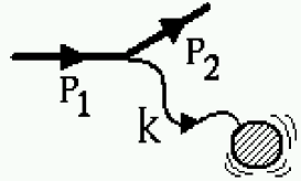
Figure 1: Long wave-length scattering: sub-structure is not seen.

In the large $k$ (short wave-length) regime, the fields depend on coordinates $X$, and so the sub-structure responsible for non-commutativity should be probed; Fig.2. As we recalled previously, in fact it is understood that the non-commutativity of D0-brane coordinates is the consequence of the strings which are stretched between D0-branes. So, by these kinds of scattering processes one should be able to probe both D0-branes (as point-like objects), and the strings stretched between them.

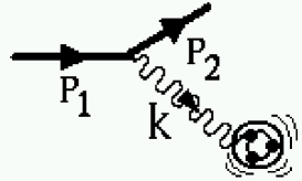
Figure 2: Short wave-length scattering: non-commutativity is probed.

Acknowledgment: I am grateful to M. Hajirahimi for her careful reading of the manuscript.

References

- [1] J. Polchinski, “Dirichlet-Branes And Ramond-Ramond Charges,” Phys. Rev. Lett. 75 (1995) 4724, hep-th/9510017.
- [2] J. Polchinski, “TASI Lectures On D-Branes,” hep-th/9611050
- [3] E. Witten, “Bound States Of Strings And -Branes,” Nucl. Phys. B460 (1996) 335, hep-th/9510135.
- [4] R.C. Myers, “Dielectric-Branes,” JHEP 9912 (1999) 022, hep-th/9910053.
- [5] W. Taylor and M. Van Raamsdonk, “Multiple Dp-Branes In Weak Background Fields,” Nucl. Phys. B573 (2000) 703, hep-th/9910052.
- [6] A.H. Fatollahi, “On Non-Abelian Structure From Matrix Coordinates,” Phys. Lett. B512 (2001) 161, hep-th/0103262.
- [7] N. Seiberg and E. Witten, “String Theory And Noncommutative Geometry,” JHEP 9909 (1999) 032, hep-th/9908142.
- [8] A. Connes, M.R. Douglas and A. Schwarz, “Noncommutative Geometry And Matrix Theory: Compactification On Tori,” JHEP 9802 (1998) 003, hep-th/9711162; M.R. Douglas and C. Hull, “D-Branes And The Noncommutative Torus,” JHEP 9802 (1998) 008, hep-th/9711165.
- [9] M.M. Sheikh-Jabbari, “Super Yang-Mills Theory On Noncommutative Torus From Open Strings Interactions,” Phys. Lett. B450 (1999) 119, hep-th/9810179.
- [10] A.H. Fatollahi, “Gauge Symmetry As Symmetry Of Matrix Coordinates,” Euro. Phys. J. C17 (2000) 535, hep-th/0007023.
- [11] A.H. Fatollahi, “D0-Branes As Confined Quarks,” talk given at “Isfahan String Workshop 2000, May 13-14, Iran,” hep-th/0005241.
- [12] A.H. Fatollahi, “D0-Branes As Light-Front Confined Quarks,” Euro. Phys. J. C19 (2001) 749, hep-th/0002021.
- [13] A.H. Fatollahi, “Do Quarks Obey D-Brane Dynamics?,” Europhys. Lett. 53(3) (2001) 317, hep-ph/9902414; “Do Quarks Obey D-Brane Dynamics?II,” hep-ph/9905484, to appear in Europhys. Lett.