Duality and Enhanced Gauge Symmetry in 2+1 Dimensions

Taichi Itoh^∗, Phillial Oh^†, and Cheol Ryou^†

^∗Department of Physics, Kyungpook National University, Taegu 702-701, Korea
^†Department of Physics and Institute of Basic Science, Sungkyunkwan University, Suwon 440-746, Korea

Abstract

We investigate the enlarged CP(N) model in 2+1 dimensions. This is a hybrid of two CP(N) models coupled with each other in a dual symmetric fashion, and it exhibits the gauge symmetry enhancement and radiative induction of the finite off-diagonal gauge boson mass as in the 1+1 dimensional case. We solve the mass gap equations and study the fixed point structure in the large-N limit. We find an interacting ultraviolet fixed point which is in contrast with the 1+1 dimensional case. We also compute the large-N effective gauge action explicitly.

PACS Numbers: 11.15.-q, 11.30.Qc, 11.10.Gh, 11.15.Pg

SKKUPT-04/2001, April 2001

1 Introduction

The nonlinear sigma models have proved to be a very useful theoretical laboratory to study many important asymptotsubjects such as spontaneous symmetry breaking [1, 2], asymptotic freedom and instantons in QCD [3, 4, 5], the dynamical generation of gauge bosons [6], target space duality in string theory [7, 8], and many others [9]. Recently, some new properties have been explored in relation with the dynamical generation of gauge bosons, that is, the gauge symmetry enhancement and radiatively induced finite gauge boson mass in 1+1 dimensions [10]. It is well-known that the $CP(N)\equiv SU(N)/SU(N-1)\times U(1)$ model [11] is the prototype of nonlinear sigma model with dynamical generation in which the auxiliary $U(1)$ gauge field becomes dynamical through the radiative corrections in the large-$N$ limit [6]. In the recently proposed extension [10] of the $CP(N)$ model, two complex projective spaces with different coupling constants have mutual interactions which are devised in such a way to preserve the duality between the two spaces. In addition to the two auxiliary $U(1)$ gauge fields which stand for each complex projective space, one extra auxiliary complex gauge field is introduced to derive the interactions with duality. It turns out that when the two coupling constants are equal, the extended model becomes the nonlinear sigma model with the target space of Grassmann manifold $Gr(N,2)=SU(N)/SU(N-2)\times U(2)$ [12].

It was shown in Ref. [10] that together with the two auxiliary $U(1)$ gauge fields this complex field becomes dynamical through radiative corrections. Moreover, in the self-dual limit where the two running coupling constants become equal, they become massless and combine with the two $U(1)$ fields to yield the $U(2)$ Yang-Mills theory. That is, the gauge symmetry enhancement has occurred in the self-dual limit. Away from this limit, the complex gauge field becomes massive. It was noted that this mass is radiatively induced through the loop corrections, and it assumes a finite value which is independent of the regularization scheme employed. This could provide an alternative approach of providing the gauge boson mass to the conventional Higgs mechanism. Therefore, it is important to attempt to extend the previous 1+1 dimensions results of Ref. [10] in order to check whether this is also viable in various other dimensions. In this paper, we take a first step, and extend the previous analysis to 2+1 dimensions. Even though the 3+1 dimensional analysis awaits for some realistic applications, it has to be recalled that the $CP(N)$ model in 2+1 dimensions [13] has many extra interesting properties such as non-perturbative renormalizability despite of appearance of linear divergence, a non-trivial UV fixed point and second order phase transition [14], and the induction of the Maxwell-Chern-Simons theory through the higher derivative interactions of renormalizable Wess-Zumino-Witten model [15]. Therefore, the analysis carried out in this paper is expected to shed light on the new aspects of 2+1 dimensional nonlinear sigma model in its own right.

The content of the paper is organized as follows. In Section 2, we review the classical feature of the coupled dual $CP(N)$ model, and elaborate on the model in terms of coadjoint orbit approach. In Section 3, we solve the large $N$ mass gap equations, and find that there exist four phases of second order phase transition which are separated by UV fixed lines. In Section 4, we discuss large $N$ renormalization and fixed point structure of the vacua. In Section 5, we carry out the path integration explicitly, and compute the $U(1)\times U(1)$ gauge invariant effective action in the unbroken phase. We show that the two point vacuum polarization graphs yield finite mass terms for the gauge fields which vanish at the self-dual limit, and the gauge symmetry is enhanced to $U(2)$ symmetry. Section 6 includes conclusion and discussion. The dimensional regularization of vacuum polarization function is presented in Appendix A. We will show the detail of three- and four-point gauge vertices in Appendix B in the space-time dimensionality $2\leq D\leq 4$.

2 Model and symmetry

We start from the Lagrangian written in terms of the $N\times 2$ matrix $Z$ such that [10]

$${\cal L}=\frac{1}{g^{2}}{\rm tr}\left[(D_{\mu}Z)^{\dagger}(D^{\mu}Z)-\lambda(Z^{\dagger}Z-R)\right],$$ (2.1)

where $\lambda$ is a $2\times 2$ hermitian matrix which transforms as an adjoint representation under the local $U(2)$ transformation. The $R$ is a $2\times 2$ matrix given by

$$R=\left[\,{r\atop 0}\quad{0\atop r^{-1}}\right],$$ (2.2)

with a real positive $r$. The covariant derivative is defined consistently as $D_{\mu}Z\equiv\partial_{\mu}Z-Z\tilde{A}_{\mu}$ with a $2\times 2$ anti-hermitian matrix gauge potential $\tilde{A}_{\mu}\equiv-i\tilde{A}_{\mu}^{a}T^{a}$ associated with the local $U(2)$ symmetry. We assign each components of $\lambda$ and $\tilde{A}_{\mu}$ as follows.

$$\lambda=\left[\,{\lambda_{1}\atop\lambda_{3}^{*}}\quad{\lambda_{3}\atop\lambda_{2}}\right],\quad\tilde{A}_{\mu}=-i\left[\,{A_{\mu}\atop\frac{1}{2}C_{\mu}^{*}}\quad{\frac{1}{2}C_{\mu}\atop B_{\mu}}\right].$$ (2.3)

The $Z$ field is made from two complex $N$-vectors $\psi_{1}$ and $\psi_{2}$ such that

$$Z=\left[\psi_{1},\psi_{2}\right],\quad\longleftrightarrow\quad Z^{\dagger}=\left[{\psi_{1}^{\dagger}\atop\psi_{2}^{\dagger}}\right].$$ (2.4)

The kinetic term of the Lagrangian (2.1) is invariant under the local $U(2)$ transformation, while the $R$ with $r\neq 1$ explicitly breaks the $U(2)$ gauge symmetry down to $U(1)_{A}\times U(1)_{B}$ where $U(1)_{A}$ and $U(1)_{B}$ are generated by $T^{0}\pm T^{3}$, respectively. Thus the symmetry of our model is $[SU(N)]_{\rm global}\times[U(2)]_{\rm local}$ for $r=1$, while $[SU(N)]_{\rm global}\times[U(1)_{A}\times U(1)_{B}]_{\rm local}$ for $r\neq 1$. The local symmetry group $H$ is $U(2)$ when $r=1$, and $U(1)_{A}\times U(1)_{B}$ when $r\neq 1$. To see the geometry of target space, we rewrite the Lagrangian (2.1) in terms of two coupling constant $g_{1}$ and $g_{2}$ defined by $g\equiv\sqrt{g_{1}g_{2}}$ and $r\equiv g_{2}/g_{1}$. Using the on-shell constraint $Z^{\dagger}Z=R$ and rescaling the fields by

$$\frac{\psi_{1}}{g}\rightarrow\frac{\psi_{1}}{g_{1}},~{}\frac{\psi_{2}}{g}\rightarrow\frac{\psi_{2}}{g_{2}},~{}\frac{C_{\mu}}{g}\rightarrow C_{\mu},~{}\frac{C_{\mu}^{*}}{g}\rightarrow C_{\mu}^{*},$$ (2.5)

the Lagrangian (2.1) can be rewritten as

$${\cal L} = \frac{1}{g_{1}^{2}}|(\partial_{\mu}+iA_{\mu})\psi_{1}|^{2}+\frac{1}{g_{2}^{2}}|(\partial_{\mu}+iB_{\mu})\psi_{2}|^{2}+\frac{1}{4}\left(\frac{g_{1}}{g_{2}}+\frac{g_{2}}{g_{1}}\right)C_{\mu}^{*}C^{\mu}$$

$$-i\frac{1}{\sqrt{g_{1}g_{2}}}C_{\mu}^{*}\psi_{1}^{\dagger}\partial^{\mu}\psi_{2}-i\frac{1}{\sqrt{g_{1}g_{2}}}C_{\mu}\psi_{2}^{\dagger}\partial^{\mu}\psi_{1}-\frac{\lambda_{3}^{*}}{g_{1}g_{2}}\psi_{1}^{\dagger}\psi_{2}-\frac{\lambda_{3}}{g_{1}g_{2}}\psi_{2}^{\dagger}\psi_{1}$$

$$-\frac{\lambda_{1}}{g_{1}^{2}}(\psi_{1}^{\dagger}\psi_{1}-1)-\frac{\lambda_{2}}{g_{2}^{2}}(\psi_{2}^{\dagger}\psi_{2}-1).$$

The above Lagrangian describes two $CP(N)$ models each described by $\psi_{1}$, $g_{1}$ and $\psi_{2},g_{2}$ coupled through the derivative coupling. There is a manifest dual symmetry between sectors 1 and 2, $A_{\mu}$ and $B_{\mu}$, $C_{\mu}$ and $C^{*}_{\mu}$, and $\lambda_{3}$ and $\lambda_{3}^{*}$. Eliminating the auxiliary fields through the equations of motion, and substituting back into the Lagrangian, we obtain modulo the on-shell constraints

$${\cal L}^{\prime}=\sum_{i=1}^{2}\frac{1}{g_{i}^{2}}\left[|\partial_{\mu}\psi_{i}|^{2}+(\psi_{i}^{\dagger}\partial_{\mu}\psi_{i})(\psi_{i}^{\dagger}\partial_{\mu}\psi_{i})\right]+\frac{2}{q}\sum_{i,j=1}^{2}{{}^{\prime}}\frac{1}{g_{i}g_{j}}(\psi_{i}^{\dagger}\partial_{\mu}\psi_{j})(\psi_{j}^{\dagger}\partial_{\mu}\psi_{i}),$$ (2.7)

where $q=g_{2}/g_{1}~{}+g_{1}/g_{2}$ and the prime in the third sum denotes that the sum is restricted to $i\neq j$ indices. We notice that the target space geometry of the Lagrangian (2.7) with $q=2$ can be understood in the coadjoint orbit approach [16, 17] to nonlinear sigma model. In terms of coadjoint orbit variables

$$Q=\frac{1}{i}\sum_{i=1}^{2}\frac{1}{g_{i}}\left(\psi_{i}\psi_{i}^{\dagger}-\frac{1}{N}I\right),~{}~{}~{}~{}\psi_{i}^{\dagger}\psi_{j}=\delta_{ij},$$ (2.8)

the Lagrangian (2.7) with $q=2$ can be rewritten as

$${\cal L}_{Q}=-\frac{1}{2}\mbox{tr}(\partial_{\mu}Q)^{2}.$$ (2.9)

In the above Lagrangian (2.9), the equal coupling $g_{1}=g_{2}$ corresponds the target space of Grassmann manifold $Gr(N,2)$, whereas the non-equal couplings $g_{1}\neq g_{2}$ to the flag manifold ${\cal M}=SU(N)/SU(N-2)\times U(1)\times U(1)$ [18]. Therefore, the generic $q\neq 2$ case of the Lagrangian (2.7) is a deformation of the flag manifold model.

In order to carry out the path integration in the large $N$ limit, we rewrite the Lagrangian (2.1) in terms of a $2\times 2$ hermitian matrix such that

$${\cal L}=\frac{1}{g^{2}}\,[\psi_{1}^{\dagger},\psi_{2}^{\dagger}]\,(M^{T}\otimes I)\left[{\psi_{1}\atop\psi_{2}}\right]+\frac{r}{g^{2}}\lambda_{1}+\frac{1}{rg^{2}}\lambda_{2},$$ (2.10)

where $\langle\cdots\rangle$ denotes a trace of an $N\times N$ matrix. The $2\times 2$ matrix operator $M$ is given by

$$M \equiv G^{-1}-\Gamma(\tilde{A}),$$ (2.11)

$$G^{-1} \equiv -\Box-\lambda\,\,=\,\,\left[\,{-\Box-\lambda_{1}\atop-\lambda_{3}^{*}}\quad{-\lambda_{3}\atop-\Box-\lambda_{2}}\right],$$ (2.12)

$$\Gamma(\tilde{A}) \equiv -\tilde{A}_{\mu}\hat{\partial}^{\mu}+\tilde{A}_{\mu}\tilde{A}^{\mu}.$$ (2.13)

where the differential operator $\hat{\partial}^{\mu}\equiv\partial^{\mu}-\overleftarrow{\partial^{\mu}}$ must be regarded as not operating on the gauge potential $\tilde{A}_{\mu}$. In terms of $A_{\mu}$, $B_{\mu}$ and $C_{\mu}$ fields, all components of the matrix $M$ are written as

$$M_{11} = -\partial^{2}-\lambda_{1}-iA_{\mu}\hat{\partial}^{\mu}+A_{\mu}A^{\mu}+\frac{1}{4}C_{\mu}^{*}C^{\mu},$$ (2.14)

$$M_{22} = -\partial^{2}-\lambda_{2}-iB_{\mu}\hat{\partial}^{\mu}+B_{\mu}B^{\mu}+\frac{1}{4}C_{\mu}^{*}C^{\mu},$$ (2.15)

$$M_{12} = -\lambda_{3}-\frac{1}{2}iC_{\mu}\hat{\partial}^{\mu}+\frac{1}{2}C_{\mu}(A^{\mu}+B^{\mu}),$$ (2.16)

$$M_{21} = -\lambda_{3}^{*}-\frac{1}{2}iC_{\mu}^{*}\hat{\partial}^{\mu}+\frac{1}{2}C_{\mu}^{*}(A^{\mu}+B^{\mu}).$$ (2.17)

Here we have never used the on-shell constraint so that the quadratic term of $C_{\mu}^{*}C^{\mu}$ has been absorbed into the matrix $M$. The last terms in Eqs. (2.16) and (2.17) were missing in the Lagrangian (2) due to the on-shell constraint but they are essential to recover the gauge invariance of the off-shell Lagrangian (2.10). We use the off-shell Lagrangian (2.10) in order to preserve the gauge invariance in every step of computation.

3 Large-N gap equations

The large $N$ effective action is given by path integrating $Z$ and $Z^{\dagger}$, or equivalently $\psi_{1}$, $\psi_{1}^{\dagger}$, $\psi_{2}$, and $\psi_{2}^{\dagger}$. We obtain

$$S_{\rm eff}=\int_{x}{\cal L}+iN\ln{\rm Det}M.$$ (3.1)

The global $U(N)$ symmetry enables us to choose the VEV vectors $\langle\psi_{1}\rangle$ and $\langle\psi_{2}\rangle$ to be real $N$-vectors and we can set all $\lambda_{1}$, $\lambda_{2}$, and $\lambda_{3}$ to be real without loss of generality. The large-$N$ effective action is determined as

$$V_{\rm eff}=-\frac{1}{N\Omega}S_{\rm eff}[\psi_{1,2}=\vec{v}_{1,2},\lambda_{1,2,3}=m^{2}_{1,2,3},\tilde{A}_{\mu}=0],$$ (3.2)

where $\vec{v}_{1}$, $\vec{v}_{2}$ are real $N$-vectors and $\Omega$ denotes the space-time volume. We obtain

$$V_{\rm eff}=\frac{m^{2}_{1}}{Ng^{2}}(\vec{v}_{1}^{2}-r)+\frac{m^{2}_{2}}{Ng^{2}}(\vec{v}_{2}^{2}-r^{-1})+\frac{2m^{2}_{3}}{Ng^{2}}\vec{v}_{1}\cdot\vec{v}_{2}-i\Omega^{-1}\ln{\rm Det}\,G^{-1},$$ (3.3)

The gap equations are schematically given as follows.

$$\frac{\partial V_{\rm eff}}{\partial\vec{v}_{1}} = \frac{2}{Ng^{2}}(m^{2}_{1}\vec{v}_{1}+m^{2}_{3}\vec{v}_{2})=0,$$ (3.4)

$$\frac{\partial V_{\rm eff}}{\partial\vec{v}_{2}} = \frac{2}{Ng^{2}}(m^{2}_{2}\vec{v}_{2}+m^{2}_{3}\vec{v}_{1})=0,$$ (3.5)

$$\frac{\partial V_{\rm eff}}{\partial m^{2}_{3}} = \frac{2}{Ng^{2}}\vec{v}_{1}\cdot\vec{v}_{2}-\int\!\frac{d^{D}k}{(2\pi)^{D}}\frac{2m^{2}_{3}}{(k^{2}+m^{2}_{+})(k^{2}+m^{2}_{-})}=0,$$ (3.6)

$$\frac{\partial V_{\rm eff}}{\partial m^{2}_{1}} = \frac{1}{Ng^{2}}(\vec{v}_{1}^{2}-r)+\int\!\frac{d^{D}k}{(2\pi)^{D}}\frac{k^{2}+m^{2}_{2}}{(k^{2}+m^{2}_{+})(k^{2}+m^{2}_{-})}=0,$$ (3.7)

$$\frac{\partial V_{\rm eff}}{\partial m^{2}_{2}} = \frac{1}{Ng^{2}}(\vec{v}_{2}^{2}-r^{-1})+\int\!\frac{d^{D}k}{(2\pi)^{D}}\frac{k^{2}+m^{2}_{1}}{(k^{2}+m^{2}_{+})(k^{2}+m^{2}_{-})}=0,$$ (3.8)

where the loop momenta are euclideanized and $m^{2}_{\pm}$ are given in terms of $m^{2}_{1,2,3}$ by

$$m^{2}_{+}+m^{2}_{-}=m^{2}_{1}+m^{2}_{2},\quad m^{2}_{+}m^{2}_{-}=m^{2}_{1}m^{2}_{2}-m^{4}_{3}.$$ (3.9)

We focus on $D=3$ case below.

First we have to regularize the divergent integrals in the gap equations. We separate out the ultraviolet divergence in (3.7) such that

$$\int^{\Lambda}\!\frac{d^{D}k}{(2\pi)^{3}}\frac{1}{k^{2}}+\int\!\frac{d^{D}k}{(2\pi)^{3}}\left[\frac{k^{2}+m^{2}_{2}}{(k^{2}+m^{2}_{+})(k^{2}+m^{2}_{-})}-\frac{1}{k^{2}}\right],$$ (3.10)

which is calculated to be

$$\frac{1}{2\pi^{2}}\Lambda-\frac{1}{4\pi}\frac{m^{2}_{1}+m_{+}m_{-}}{m_{+}+m_{-}}.$$ (3.11)

Then we obtain the properly regularized gap equations in $D=3$:

$$m^{2}_{1}\vec{v}_{1}+m^{2}_{3}\vec{v}_{2} = 0,$$ (3.12)

$$m^{2}_{2}\vec{v}_{2}+m^{2}_{3}\vec{v}_{1} = 0,$$ (3.13)

$$\frac{1}{u}\Lambda\,\vec{v}_{1}\cdot\vec{v}_{2} = \frac{1}{4\pi}\frac{m^{2}_{3}}{m_{+}+m_{-}},$$ (3.14)

$$\frac{1}{u}\Lambda\,\vec{v}_{1}^{2} = \left(\frac{r}{u}-\frac{1}{u^{*}}\right)\Lambda+\frac{1}{4\pi}\frac{m^{2}_{1}+m_{+}m_{-}}{m_{+}+m_{-}},$$ (3.15)

$$\frac{1}{u}\Lambda\,\vec{v}_{2}^{2} = \left(\frac{1}{ur}-\frac{1}{u^{*}}\right)\Lambda+\frac{1}{4\pi}\frac{m^{2}_{2}+m_{+}m_{-}}{m_{+}+m_{-}},$$ (3.16)

where we have introduced the dimensionless coupling $u\equiv Ng^{2}\Lambda$ and $u^{*}\equiv 2\pi^{2}$.

Suppose that $m_{3}\neq 0$ is a solution to the gap equations. The equations (3.12) and (3.13) yield that $\vec{v}_{1}$ and $\vec{v}_{2}$ are anti-parallel to each other, say specifically,

$$\vec{v}_{2}=-\frac{m^{2}_{1}}{m^{2}_{3}}\vec{v}_{1},\quad\vec{v}_{1}=-\frac{m^{2}_{2}}{m^{2}_{3}}\vec{v}_{2},$$ (3.17)

of which iterative substitution provides $m^{2}_{3}=m_{1}m_{2}$ so that we can set $m_{+}=\sqrt{m^{2}_{1}+m^{2}_{2}}$, $m_{-}=0$. Substituting (3.17) into (3.14), we obtain

$$\frac{1}{u}\Lambda\,\vec{v}_{1}^{2}=-\frac{1}{4\pi}\frac{m_{2}^{2}}{\sqrt{m^{2}_{1}+m^{2}_{2}}}.$$ (3.18)

The left hand side is positive, whereas the right hand side is negative. This result is obviously inconsistent in itself and we therefore conclude that $m_{3}\neq 0$ is not a solution to the gap equations.

Setting $m_{3}=0$ in (3.9), we can choose for example $m_{+}=m_{1}$, $m_{-}=m_{2}$. Then the gap equations are simplified such that

$$m^{2}_{1}\vec{v}_{1} = 0,$$ (3.19)

$$m^{2}_{2}\vec{v}_{2} = 0,$$ (3.20)

$$\vec{v}_{1}\cdot\vec{v}_{2} = 0,$$ (3.21)

$$\frac{1}{u}\Lambda\,\vec{v}_{1}^{2} = \left(\frac{r}{u}-\frac{1}{u^{*}}\right)\Lambda+\frac{1}{4\pi}m_{1},$$ (3.22)

$$\frac{1}{u}\Lambda\,\vec{v}_{2}^{2} = \left(\frac{1}{ur}-\frac{1}{u^{*}}\right)\Lambda+\frac{1}{4\pi}m_{2}.$$ (3.23)

Note that $\vec{v}_{1}$ and $\vec{v}_{2}$ are perpendicular each other and may possibly break the global $SU(N)$ symmetry down to the $SU(N-2)\times U(1)\times U(1)$ symmetry.

In order to simplify the following analysis, let us introduce $u_{1}\equiv u/r$ and $u_{2}\equiv ur$. The possible phases of vacuum are classified depending on the regions in the parameter space $(u_{1},u_{2})$ as follows (See Fig. 1.).

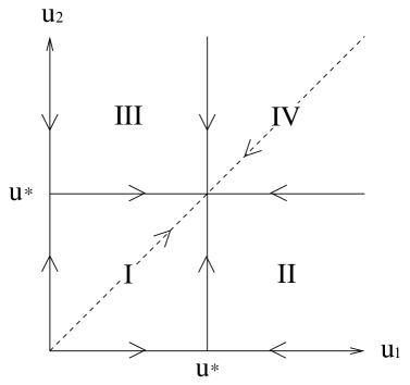
Figure 1: Large-$N$ phase diagram in three-dimensions.

• $u_{1}<u^{*}$ and $u_{2}<u^{*}$ $\,\longleftrightarrow\,$ $u/u^{*}<\min\{r,r^{-1}\}$

  Since the right hand sides of both (3.22) and (3.23) become positive in this case, we have a solution: $\vec{v}_{1}\neq\vec{0}$, $\vec{v}_{2}\neq\vec{0}$ ($m_{1}=0$, $m_{2}=0$). The orthogonal condition (3.21) tells us that this solution maximally breaks the global $SU(N)$ symmetry down to $SU(N-2)\times U(1)\times U(1)$. From Eqs. (2.14), (2.15) we see that all gauge fields become massive due to $\langle\psi_{1}^{\dagger}\psi_{1}\rangle\neq 0$ and $\langle\psi_{2}^{\dagger}\psi_{2}\rangle\neq 0$ so that the gauge group $H$ is fully broken.

• $u_{1}>u^{*}$ and $u_{2}<u^{*}$ $\,\longleftrightarrow\,$ $r<u/u^{*}<r^{-1}$

  The right hand side of (3.22) is not positive definite so that we have a solution: $\vec{v}_{1}=\vec{0}$, $\vec{v}_{2}\neq\vec{0}$ ($m_{1}\neq 0$, $m_{2}=0$). The $SU(N)$ symmetry is broken down to $SU(N-1)\times U(1)$. Eq. (2.15) tells us that $B_{\mu}$ and $C_{\mu}$ become massive due to $\langle\psi_{2}^{\dagger}\psi_{2}\rangle\neq 0$, while $A_{\mu}$ remains massless as shown in Eq. (2.14). In terms of the $U(2)$ adjoint gauge fields, $A_{\mu}$ is written as $A_{\mu}=(\tilde{A}^{0}_{\mu}+\tilde{A}^{3}_{\mu})/2$ and is therefore regarded as a gauge filed associated with the $U(1)_{A}$ gauge symmetry. The local $H$ symmetry is broken down to the $U(1)_{A}$ symmetry.

• $u_{1}<u^{*}$ and $u_{2}>u^{*}$ $\,\longleftrightarrow\,$ $r^{-1}<u/u^{*}<r$

  As the case before we have a solution: $\vec{v}_{1}\neq\vec{0}$, $\vec{v}_{2}=\vec{0}$ ($m_{1}=0$, $m_{2}\neq 0$). The $SU(N)$ symmetry is broken down to $SU(N-1)\times U(1)$. Since $B_{\mu}$ only remains massless, the $H$ symmetry is broken down to the $U(1)_{B}$ symmetry.

• $u_{1}>u^{*}$ and $u_{2}>u^{*}$ $\,\longleftrightarrow\,$ $u/u^{*}>\max\{r,r^{-1}\}$

  We only have a trivial solution: $\vec{v}_{1}=\vec{0}$, $\vec{v}_{2}=\vec{0}$ ($m_{1}\neq 0$, $m_{2}\neq 0$). Both global $SU(N)$ and local $H$ symmetries remain unbroken.

We notice that the four phases I, II, III, IV are separated by the two critical lines $u_{1}=u^{*}$ and $u_{2}=u^{*}$ which arise as ultraviolet (UV) fixed lines associated with the second order phase transitions after the large-$N$ renormalization of the effective potential.

4 Renormalization and fixed point structure of the vacua

The only UV divergences in the large-$N$ effective potential are those in the gap equations (3.22), (3.23) so that we impose the following renormalization conditions:

$$\frac{d}{d\ln\Lambda}\left(\frac{1}{u_{1}}-\frac{1}{u^{*}}\right)\Lambda=0,$$ (4.1)

$$\frac{d}{d\ln\Lambda}\left(\frac{1}{u_{2}}-\frac{1}{u^{*}}\right)\Lambda=0.$$ (4.2)

This yields two decoupled renormalization group (RG) equations

$$\frac{du_{1}}{d\ln\Lambda} = u_{1}\left(1-\frac{u_{1}}{u^{*}}\right),$$ (4.3)

$$\frac{du_{2}}{d\ln\Lambda} = u_{2}\left(1-\frac{u_{2}}{u^{*}}\right),$$ (4.4)

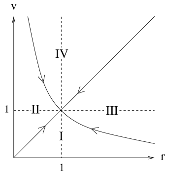
of which UV fixed points $u_{1}=u^{*}$ and $u_{2}=u^{*}$ can be identified with the two critical lines which separate the four different phases. Moreover, the intersection point $(u_{1},u_{2})=(u^{*},u^{*})$ is conformally invariant. This situation is realized as a self-dual condition $r=1$ ($u_{1}=u_{2})$ which arises as a UV fixed line of the RG $\beta$-function for $r$. In terms of $v\equiv u/u^{*}$ and $r$, the RG equations are equivalently rewritten as two coupled equations:

$$\frac{dv}{d\ln\Lambda} = v\left[1-\frac{1}{2}\left(r+\frac{1}{r}\right)v\right],$$ (4.5)

$$\frac{dr}{d\ln\Lambda} = \frac{1}{2}v\left(1-r^{2}\right),$$ (4.6)

which show two relevant directions $v=r$ and $v=r^{-1}$ around $(r,v)=(1,1)$. In fact, if we substitute $v=r$ or $v=r^{-1}$ into (4.5) and (4.6), the two equations reduce to the equations

$$\frac{dr}{d\ln\Lambda}=\left\{{\displaystyle\frac{1}{2}r(1-r^{2})\quad\mbox{for}\quad v=r,\atop\displaystyle\frac{1}{2r}(1-r^{2})\quad\mbox{for}\quad v=\frac{1}{r}.}\right.$$ (4.7)

This shows existence of the UV fixed point at $r=v=1$. The phase diagram in the $(r,v)$-plane is depicted in Fig. 2.

Figure 2: Large-$N$ phase diagram in the $(r,v)$-plane.

5 Large-N effective action and enhanced gauge symmetry

The large-$N$ effective action (3.1) is schematically expanded such that

$$S_{\rm eff}=\int_{x}{\cal L}+iN\ln{\rm Det}\,G^{-1}-iN\sum_{n=1}^{\infty}\frac{1}{n}{\rm Tr}\left[G\Gamma(\tilde{A})\right]^{n}.$$ (5.1)

The boson propagator $G$ becomes a diagonal $2\times 2$ matrix due to the gap equation solution $m_{3}=0$. We neglect the fluctuation fields coming from $\lambda_{1,2,3}$ around $m^{2}_{1,2,3}$ and consider the symmetric phase IV. In the following we study the diagrams up to four-point functions which are of the lowest order in the derivative expansion and cast into the Yang-Mills action of the enhanced $U(2)$ gauge symmetry at the self-dual limit r=1.

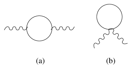
5.1 Vacuum polarization and the off-diagonal gauge boson mass

We have two diagrams in Fig. 3. They are combined into kinetic terms such that

$$\mbox{(3a)}+\mbox{(3b)} = -iN\frac{1}{2}{\rm Tr}\left[G\tilde{A}_{\mu}\hat{\partial}^{\mu}G\tilde{A}_{\nu}\hat{\partial}^{\nu}\right]-iN{\rm Tr}\left[G\tilde{A}_{\mu}\tilde{A}^{\mu}\right]$$ (5.2)

$$= \frac{N}{2}\sum_{ij}\int_{x}\,\tilde{A}^{\mu}_{ij}(x)\Pi_{\mu\nu}^{ij}(i\partial_{x})\tilde{A}^{\nu}_{ji}(x),$$

where the vacuum polarization function $\Pi$ is given by

$$\Pi_{\mu\nu}^{ij}(p)=-\int\!\frac{d^{3}k}{i(2\pi)^{3}}\frac{(2k+p)_{\mu}(2k+p)_{\nu}}{(k^{2}-m_{i}^{2})[(k+p)^{2}-m_{j}^{2}]}+\int\!\frac{d^{3}k}{i(2\pi)^{3}}\frac{2g_{\mu\nu}}{k^{2}-m_{i}^{2}}.$$ (5.3)

which must be regularized so as to preserve the $U(1)_{A}\times U(1)_{B}$ gauge invariance which is manifest even when $r\neq 1$. The vacuum polarization function is calculated such that

$$\Pi_{\mu\nu}^{ij}(p)=\left(g_{\mu\nu}-\frac{p_{\mu}p_{\nu}}{p^{2}}\right)\Pi_{T}^{ij}(p)+\left(\frac{p_{\mu}p_{\nu}}{p^{2}}\right)\Pi_{L}^{ij}(p),$$ (5.4)

with the transverse function $\Pi_{T}$ and the longitudinal one $\Pi_{L}$ obtained as (See Appendix A)

$$\Pi_{T}^{ij}(p) \equiv \frac{1}{2\pi}\left[\frac{m_{i}+m_{j}}{2}-\int_{0}^{1}dx\sqrt{K}\right],$$ (5.5)

$$\Pi_{L}^{ij}(p) \equiv \frac{\left(m_{i}^{2}-m_{j}^{2}\right)^{2}}{8\pi p^{2}}\left[\frac{2}{m_{i}+m_{j}}-\int_{0}^{1}dx\frac{1}{\sqrt{K}}\right],$$ (5.6)

where we have introduced $K\equiv xm_{i}^{2}+(1-x)m_{j}^{2}-x(1-x)p^{2}$. Each of $\Pi_{T}$ and $\Pi_{L}$ has a constant as the leading term in momentum expansion. Moreover we see that

$$\Pi_{T}^{ij}(p) = c^{ij}+p^{2}f_{T}^{ij}(p),$$ (5.7)

$$\Pi_{L}^{ij}(p) = c^{ij}+p^{2}f_{L}^{ij}(p),$$ (5.8)

where the same constant $c^{ij}$ arises both in $\Pi_{T}$ and $\Pi_{L}$ and is determined as

$$c^{ij}=-\frac{(m_{i}-m_{j})^{2}}{12\pi(m_{i}+m_{j})}.$$ (5.9)

Then the vacuum polarization can be written as

$$\Pi_{\mu\nu}^{ij}(p)=c^{ij}g_{\mu\nu}+(p^{2}g_{\mu\nu}-p_{\mu}p_{\nu})f_{T}^{ij}(p)+p_{\mu}p_{\nu}f_{L}^{ij}(p),$$ (5.10)

where both $c^{ij}$ and $f_{L}^{ij}$ vanish when $i=j$ so as to provide the $A$ ($B$) boson with the $U(1)_{A}$ ($U(1)_{B}$) gauge invariant kinetic term, while they remain nonzero when $i\neq j$ and provide the $C$ boson with the mass given by (See Appendix A)

$$M_{C}=\sqrt{\frac{-c^{12}}{f_{T}^{12}(0)}}=\left|\frac{m_{1}^{2}-m_{2}^{2}}{2}\right|\sqrt{\frac{5}{m_{1}^{2}+m_{2}^{2}+3m_{1}m_{2}}}.$$ (5.11)

A couple of remarks are in order. Firstly, we note that the above mass does not vanishes when $m_{1}\neq m_{2}$ which in turn implies $r\neq 1$ from the mass gap equations (3.22) and (3.23). It is also symmetric under the exchange of $m_{1}$ and $m_{2}$. At the self-dual limit $r=1$ ($m_{1}=m_{2}=m$), both $c^{12}$ and $\tilde{\Pi}_{L}^{12}$ become zero so that the off-diagonal $C$ boson becomes massless and combines into the enhanced $U(2)$ gauge fields together with the diagonal $A$, $B$ bosons. Secondly, it should be emphasized that this mass generation of $C$ bosons is a genuine quantum effect away from the self-dual line and the mass takes a definite value in terms of the two mass scales without any ambiguity. It is also independent of the regularization scheme employed. This unambiguity is in contrast with some other radiative corrections in quantum field theory which are finite but undetermined [19].

The vacuum polarization diagrams in Fig. 3 finally provide the kinetic terms

$$\mbox{(3a)}+\mbox{(3b)} = \frac{N}{4}\int_{x}~{}\Biggl{[}-f_{T}^{11}(0)F_{\mu\nu}F^{\mu\nu}(A)-f_{T}^{22}(0)F_{\mu\nu}F^{\mu\nu}(B)-c^{12}C^{\mu}C_{\mu}^{*}$$ (5.12)

$$-\frac{1}{2}f_{T}^{12}(0)\partial_{[\mu}C_{\nu]}^{*}~{}\partial^{[\mu}C^{\nu]}-f_{L}^{12}(0)\partial^{\mu}C^{*}_{\mu}\partial^{\nu}C_{\nu}\Biggr{]}.$$

in the leading order of derivative expansion. At the self-dual limit, $f_{T}^{11}(0)=f_{T}^{22}(0)=N/24\pi m$ and $c^{12}$, $f_{L}^{12}(0)\to 0$ so that the above kinetic terms are rearranged into

$$\mbox{(3a)}+\mbox{(3b)}=\frac{N}{96\pi m}\int_{x}\left[{\rm tr}\left\{\partial_{[\mu}\tilde{A}_{\nu]}\partial^{[\mu}\tilde{A}^{\nu]}\right\}+O(\partial^{2}\frac{\partial^{2}}{m^{2}})\right].$$ (5.13)

Figure 3: Vacuum polarization diagrams. (a) $n=2$. (b) $n=1$.

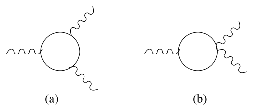
5.2 Three-point gauge vertices

Both of three-point gauge diagrams (a) and (b) in Fig. 4 contribute to the Yang-Mills action. They are given by the following integrals:

(4a) $$= iN\frac{1}{3}{\rm Tr}\left[G\tilde{A}_{\mu}\hat{\partial}^{\mu}G\tilde{A}_{\nu}\hat{\partial}^{\nu}G\tilde{A}_{\rho}\hat{\partial}^{\rho}\right],$$ (5.14)

(4b) $$= iN{\rm Tr}\left[G\tilde{A}_{\mu}\hat{\partial}^{\mu}G\tilde{A}_{\nu}\tilde{A}^{\nu}\right].$$ (5.15)

In the leading order of derivative expansion, they are calculated to be (See Appendix B)

$$\mbox{(4a)}+\mbox{(4b)} = \frac{iN}{4}f_{T}^{12}(0)\int_{x}~{}\Biggl{[}-\frac{1}{2}\Bigl{(}W_{[\mu}C_{\nu]}^{*}\partial^{[\mu}C^{\nu]}-\partial_{[\mu}C_{\nu]}^{*}W^{[\mu}C^{\nu]}\Bigr{)}$$ (5.16)

$$-\frac{2}{3}(b_{1}+b_{2}\Bigr{)}\Bigl{(}W_{\mu}C^{*}_{\nu}\partial^{\nu}C^{\mu}-\partial_{\mu}C^{*}_{\nu}W^{\nu}C^{\mu}\Bigr{)}$$

$$-\frac{1}{3}\left(b_{1}-2b_{2}\right)\Bigl{(}W_{\mu}C^{*\mu}\partial_{\nu}C^{\nu}-\partial_{\mu}C^{*\mu}W_{\nu}C^{\nu}\Bigr{)}$$

$$-\Bigl{(}1-\frac{b_{1}}{3}-\frac{b_{2}}{3}\Bigr{)}C^{\nu}C^{*\mu}F_{\mu\nu}(A)-\Bigl{(}1-\frac{b_{1}}{3}+\frac{b_{2}}{3}\Bigr{)}C^{*\nu}C^{\mu}F_{\mu\nu}(B)\Biggr{]},$$

where we have defined $b_{1}$, $b_{2}$ and $W_{\mu}$ such that

$$b_{1}\equiv\frac{f_{L}^{12}(0)}{f_{T}^{12}(0)},\quad b_{2}\equiv\frac{M_{C}^{2}}{m_{1}^{2}-m_{2}^{2}},\quad W_{\mu}\equiv A_{\mu}-B_{\mu}.$$ (5.17)

At the self-dual limit $r=1$ ($m_{1}=m_{2}=m$), Eq. (5.16) turns to the following simple form

$$\mbox{(4a)}+\mbox{(4b)}=\frac{N}{48\pi m}\int_{x}\left[{\rm tr}\left\{\partial_{[\mu}\tilde{A}_{\nu]}[\tilde{A}^{\mu},\tilde{A}^{\nu}]\right\}+O(\partial\frac{\partial^{2}}{m^{2}})\right].$$ (5.18)

Figure 4: Three-point gauge vertices. (a) $n=3$. (b) $n=2$.

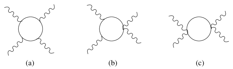
5.3 Four-point gauge vertices

The four-point gauge diagrams which contribute to the Yang-Mills action are shown in Fig. 5. They are given by the following integrals:

(5a) $$= -iN\frac{1}{4}{\rm Tr}\left[G\tilde{A}_{\mu}\hat{\partial}^{\mu}G\tilde{A}_{\nu}\hat{\partial}^{\nu}G\tilde{A}_{\rho}\hat{\partial}^{\rho}G\tilde{A}_{\sigma}\hat{\partial}^{\sigma}\right],$$ (5.19)

(5b) $$= -iN{\rm Tr}\left[G\tilde{A}_{\mu}\hat{\partial}^{\mu}G\tilde{A}_{\nu}\hat{\partial}^{\nu}G\tilde{A}_{\rho}\tilde{A}^{\rho}\right],$$ (5.20)

(5c) $$= -iN\frac{1}{2}{\rm Tr}\left[G\tilde{A}_{\mu}\tilde{A}^{\mu}G\tilde{A}_{\nu}\tilde{A}^{\nu}\right].$$ (5.21)

Calculation of the above integrals in the leading order of derivative expansion yields (See Appendix B)

$$\mbox{(5a)}+\mbox{(5b)}+\mbox{(5c)} = \frac{N}{4}f_{T}^{12}(0)\int_{x}~{}\Biggl{[}-\frac{1}{2}W_{[\mu}C_{\nu]}^{*}W^{[\mu}C^{\nu]}-b_{1}W_{\mu}C^{*\mu}W_{\nu}C^{\nu}$$ (5.22)

$$+\frac{1}{4}C^{\mu}C_{\mu}C^{*\nu}C_{\nu}^{*}-\frac{1}{2}\Bigl{(}2-b_{1}-\frac{3}{4}b_{3}\Bigr{)}C^{\mu}C_{\mu}^{*}C^{\nu}C_{\nu}^{*}\Biggr{]}.$$

where we have defined $b_{3}$ as

$$b_{3}\equiv\frac{f_{T}^{11}(0)+f_{T}^{22}(0)}{f_{T}^{12}(0)}.$$ (5.23)

At the self-dual limit, Eq. (5.22) is simplified to be the following form

$$\mbox{(5a)}+\mbox{(5b)}+\mbox{(5c)}=\frac{N}{96\pi m}\int_{x}\left[{\rm tr}\left\{[\tilde{A}_{\mu},\tilde{A}_{\nu}][\tilde{A}^{\mu},\tilde{A}^{\nu}]\right\}+O(\frac{\partial^{2}}{m^{2}})\right].$$ (5.24)

Figure 5: Four-point gauge vertices. (a) $n=4$. (b) $n=3$. (c) $n=2$.

5.4 Large-N effective action and the equations of motion

Combining Eqs. (5.12), (5.16) and (5.22), we obtain the $U(1)_{A}\times U(1)_{B}$ gauge invariant effective action

$${\cal L}_{\rm eff} = -\frac{1}{4{g_{A}}^{2}}F_{\mu\nu}F^{\mu\nu}(A)-\frac{1}{4{g_{B}}^{2}}F_{\mu\nu}F^{\mu\nu}(B)+M_{C}^{2}{V_{\mu}^{*}}V^{\mu}-\frac{1}{2}({\cal D}_{[\mu}V_{\nu]})^{*}({\cal D}^{[\mu}V^{\nu]})$$ (5.25)

$$-\frac{2}{3}(b_{1}+b_{2})({\cal D}_{\mu}V_{\nu})^{*}({\cal D}^{\nu}V^{\mu})-\frac{1}{3}(b_{1}-2b_{2})({\cal D}_{\mu}V^{\mu})^{*}({\cal D}_{\nu}V^{\nu})$$

$$-\Bigl{(}1-\frac{b_{1}}{3}-\frac{b_{2}}{3}\Bigr{)}iV^{\nu}V^{*\mu}F_{\mu\nu}(A)+\Bigl{(}1-\frac{b_{1}}{3}+\frac{b_{2}}{3}\Bigr{)}iV^{\nu}V^{*\mu}F_{\mu\nu}(B)$$

$$+\kappa\,V^{\mu}V_{\mu}V^{*\nu}V^{*}_{\nu}-2\kappa\,\Bigl{(}2-b_{1}-\frac{3}{4}b_{3}\Bigr{)}V^{\mu}V_{\mu}^{*}V^{\nu}V_{\nu}^{*},$$

where the gauge couplings $g_{A},g_{B}$ and the four-point coupling $\kappa$ are given by

$$g_{A}^{2}\equiv\frac{1}{Nf_{T}^{11}(0)},\quad g_{B}^{2}\equiv\frac{1}{Nf_{T}^{22}(0)},\quad\kappa\equiv\frac{1}{Nf_{T}^{12}(0)},$$ (5.26)

and ${\cal D}_{\mu}$ denotes the $U(1)_{A}\times U(1)_{B}$ covariant derivative ${\cal D}_{\mu}\equiv\partial_{\mu}-iW_{\mu}$. The $V$ field comes from the rescaling $\sqrt{Nf_{T}^{12}(0)}\,C_{\mu}\longrightarrow 2V_{\mu}$.

The field equations derived from the above Lagrangian are given as follows;

$$\partial^{\mu}F_{\mu\nu}(A)=g_{A}^{2}J^{+}_{\nu},$$ (5.27)

$$\partial^{\mu}F_{\mu\nu}(B)=g_{B}^{2}J^{-}_{\nu},$$ (5.28)

$$\partial^{\mu}F_{\mu\nu}(V)+b_{1}\partial_{\nu}\partial_{\mu}V^{\mu}+M_{C}^{2}V_{\nu}=\tilde{J}_{\nu},$$ (5.29)

where the $U(1)_{A}\times U(1)_{B}$ current $J^{\pm}_{\nu}$ and the source current for the $V$ field $\tilde{J}_{\nu}$ are given such that

$$J^{+}_{\nu} = i\Bigl{(}1-b_{1}-b_{2}\Bigr{)}\partial^{\mu}(V_{[\mu}V^{*}_{\nu]})+ib_{1}\Bigl{[}V^{*}_{\nu}\partial_{\mu}V^{\mu}-V_{\nu}\partial_{\mu}V^{*\mu}\Bigr{]}$$ (5.30)

$$+i\Bigl{[}V^{\mu}F_{\mu\nu}(V^{*})-V^{*\mu}F_{\mu\nu}(V)\Bigr{]}+(b_{1}-1)W^{\mu}V_{(\nu}V^{*}_{\mu)}+2W_{\nu}V^{*}_{\mu}V^{\mu},$$

$$J^{-}_{\nu} = -J^{+}_{\nu}-\frac{2b_{2}}{3}~{}i\partial^{\mu}(V_{[\mu}V^{*}_{\nu]}),$$ (5.31)

$$\tilde{J}_{\nu} = iW^{\mu}F_{\mu\nu}(V)+i{\cal D}^{\mu}(W_{[\mu}V_{\nu]})+ib_{1}\Bigl{[}\partial_{\nu}(W_{\mu}V^{\mu})+W_{\nu}{\cal D}_{\mu}V^{\mu}\Bigr{]}$$ (5.32)

$$-i\Bigl{(}1-b_{1}-b_{2}\Bigr{)}V^{\mu}F_{\mu\nu}(A)+i\Bigl{(}1-b_{1}-\frac{b_{2}}{3}\Bigr{)}V^{\mu}F_{\mu\nu}(B)$$

$$+4\kappa\Bigl{(}2-b_{1}-\frac{3}{4}b_{3}\Bigr{)}V^{\mu}V^{*}_{\mu}V_{\nu}-2\kappa V^{\mu}V_{\mu}V^{*}_{\nu}.$$

The first two field equations require the current conservation $\partial_{\nu}J^{\pm\nu}=0$ which we can confirm by using all the field equations together with the identity

$${\rm Im}\Bigl{[}V^{*}_{\nu}\tilde{J}^{\nu}\Bigr{]}=\frac{1}{2}\partial^{\nu}\Biggl{[}(b_{1}-1)W^{\mu}V_{(\nu}V^{*}_{\mu)}+2W_{\nu}V^{*}_{\mu}V^{\mu}\Biggr{]}.$$ (5.33)

Taking divergence of the third field equation yields

$$(b_{1}\Box+M_{C}^{2})\,\partial_{\mu}V^{\mu}=\partial_{\mu}\tilde{J}^{\mu}.$$ (5.34)

Note that the parameter $b_{1}$ is negative (See Eqs. (A.8) and (A.9) in Appendix A). Therefore, if we turn off all the interactions ($\partial_{\mu}\tilde{J}^{\mu}=0$), Eq. (5.34) tells us that the scalar mode of $V$ boson becomes a tachyon. As we will show shortly, the $V$ boson turns into the off-diagonal components of the enhanced $U(2)$ gauge bosons at the self-dual limit. In order to quantize the effective gauge theory (5.25), we have to take all the interaction terms into account even away from the self-dual points. In fact, $\partial_{\mu}\tilde{J}^{\mu}$ contains a term such as $A_{\nu}\partial^{\nu}(\partial_{\mu}V^{\mu})$ which may possibly change the tachyonic behavior of the scalar mode.

5.5 Yang-Mills action of the enhanced gauge symmetry

At the self-dual limit $r=1$, the effective action (5.25) turns into the $U(2)$ Yang-Mills action

$${\cal L}_{\rm eff}=\frac{N}{96\pi m}\,{\rm tr}\,F_{\mu\nu}F^{\mu\nu}(\tilde{A}),$$ (5.35)

where $F_{\mu\nu}(\tilde{A})\equiv\partial_{[\mu}\tilde{A}_{\nu]}+[\tilde{A}_{\mu},\tilde{A}_{\nu}]$ is the field strength of the enhanced nonabelian $U(2)$ gauge symmetry. Away from the self-dual points $m_{1}\neq m_{2}$, the effective gauge action (5.25) is no longer written as a single trace of $U(2)$ matrix. However the three-point and four-point gauge interactions still preserve the $U(1)_{A}\times U(1)_{B}$ gauge invariance.

We conclude this section by observing that the large-$N$ effective action is renormalizable in fewer than 3+1 dimensions. The only UV divergence is the one which arises in the gap equation and the other possible UV divergences in the vacuum polarization function are either forbidden by the gauge symmetry or related to the order parameters $\vec{v}_{1}$ or $\vec{v}_{2}$. The renormalization conditions (4.1) and (4.2) are enough to realize the UV finite large-$N$ theory. The higher order corrections in $1/N$-expansion can be systematically renormalized by using the counter terms which the large-$N$ effective action (3.1) suffices. Unfortunately, in 3+1 dimensions, there arises a logarithmic divergence in the large-$N$ gap equations (See Eq. (A.27) in Appendix A). This UV divergence prevents us from taking the continuum limit. To improve this involves modifying renormalization group equations by adding extra counter terms which absorb the logarithmic divergence and imposing a matching condition which requires the compositeness of dynamical gauge bosons [20, 21].

6 Conclusion and Discussion

We have performed the large $N$ path integral of a coupled $CP(N)$ model with dual symmetry and analyzed the vacuum structure and renormalization in the large-$N$ limit in 2+1 dimensions. The large-$N$ gap equation analysis yields a solution with two decoupled gap equations. Consequently, we have the dimensionless coupling constant $(u_{1},u_{2})$-plane separated into the four regions with two UV fixed lines. Then we find the breaking patterns of the global $SU(N)$ and the local $H$ symmetries which are summarized in Table 1.

Every transition between two of the four phases is the second order phase transition associated with the dynamical Higgs mechanism. However, the massive gauge boson which acquires a mass term through the Higgs mechanism is actually no longer stable and is dissociated into a pair of Nambu-Goldstone bosons (for example in the phase II, a massive $B$ boson decays into a pair of $\psi_{2}^{\dagger}$ and $\psi_{2}$). Note that the origin of $C$ boson mass is not the Higgs mechanism but rather the explicit breaking parameter $r$, the radius (or inverse radius) of $CP(N)$. The $C$ boson is therefore a propagating massive vector field even in broken phases.

We also have computed the effective gauge Lagrangian in the unbroken phase IV explicitly. The effective Lagrangian (5.25) tells us that other than dynamically generated gauge bosons $A$ and $B$, we have a propagating $C$ boson which acquires radiatively induced finite mass away from the UV fixed point. Besides, the RG analysis of Section 4 have shown that all the RG trajectories inside the phase IV flow into the self-dual UV fixed point where the two UV fixed lines intersect. Therefore we conclude that even if we start from the theory with two different $CP(N)$ radii, the theory favors the conformal fixed point with two coincident radii and the $U(1)_{A}\times U(1)_{B}$ gauge symmetry is enhanced to be a nonabelian $U(2)$ symmetry in UV limit. Note that the classical dual symmetry is not broken by the nonperturbative radiative corrections and survives in the effective action (5.25).

The dynamical generation of the $C$ boson mass considered in this paper is purely due to the finite radiative corrections, whereas the conventional dynamical Higgs mechanism is known to be unsatisfactory due to the hierarchy problem. Therefore, our results could have some realistic applications, if the present analysis could be extended to 3+1 dimensions [20, 21]. In this respect, it is useful to recall that one of the original motivations for the dynamical generation of gauge bosons through the nonlinear sigma model was to account for the gauge group which is large enough to accommodate the known standard model in ${\cal N}=8$ extended supergravity theory [22]. However, this theory has, although large enough, a non-compact sigma model sector and progress along this direction has been hampered by the no-go theorem [23] which states that the dynamical generation of gauge bosons does not occur for the non-compact target spaces. Therefore, it remains to be a challenging problem to overcome [24] the no-go theorem and extend our results to non-compact nonlinear sigma model in 3+1 dimensions.

phase	$[SU(N)]_{\rm global}$	$[H]_{\rm local}$
I.	$SU(N-2)\times U(1)\times U(1)$	fully broken
II.	$SU(N-1)\times U(1)$	$U(1)_{A}$
III.	$SU(N-1)\times U(1)$	$U(1)_{B}$
IV.	$SU(N)$ unbroken	$U(1)_{A}\times U(1)_{B}$ unbroken

Table 1: The breaking patterns of the global $SU(N)$ and the local $H$ symmetries.

T.I. was supported by the grant of Post-Doc. Program, Kyungpook National University (2000). P.O. was supported by the Korea Research Foundation through project number DP0087.

Appendix Appendix A Dimensional regularization

Throughout the calculation of vacuum polarization function and three- and four-point functions, we have used dimensional regularization which is simply calculating Feynman integrals in the space-time dimensionality $2\leq D\leq 4$. Two-dimensional results are obtained by introducing a small parameter $\epsilon\equiv(D-2)/2$ and taking the limit $\epsilon\to 0$. If we use another small parameter $\tilde{\epsilon}\equiv(4-D)/2$ and take the limit $\tilde{\epsilon}\to 0$, we can see four-dimensional results also.

The vacuum polarization function in $D$ dimensions is given by the same Feynman integral (5.3), except that the momentum integration is now $D$-dimensional, and is calculated such that

$$\Pi_{\mu\nu}^{ij}(p)=\left(g_{\mu\nu}-\frac{p_{\mu}p_{\nu}}{p^{2}}\right)\Pi_{T}^{ij}(p)+\left(\frac{p_{\mu}p_{\nu}}{p^{2}}\right)\Pi_{L}^{ij}(p),$$ (A.1)

with the transverse and longitudinal functions $\Pi_{T}$, $\Pi_{L}$ which are obtained in $D$ dimensions as

$$\Pi_{T}^{ij}(p) = \eta_{D}\Biggl{[}\frac{4}{D-2}\Biggr{]}\Biggl{[}\frac{\,m_{i}^{D-2}+m_{j}^{D-2}}{2}-\int_{0}^{1}dxK^{\frac{D-2}{2}}\Biggr{]}$$ (A.2)

$$\Pi_{L}^{ij}(p) = \eta_{D}\Biggl{[}\frac{\left(m_{i}^{2}-m_{j}^{2}\right)^{2}}{p^{2}}\Biggr{]}\Biggl{[}\frac{2}{D-2}\frac{\,m_{i}^{D-2}-m_{j}^{D-2}}{m_{i}^{2}-m_{j}^{2}}-\int_{0}^{1}dxK^{\frac{D-4}{2}}\Biggr{]}$$ (A.3)

where $K\equiv xm_{i}^{2}+(1-x)m_{j}^{2}-x(1-x)p^{2}$ and $\eta_{D}\equiv\Gamma(2-{D\over 2})/(4\pi)^{D\over 2}$. Actually, the vacuum polarization function $\Pi^{ij}_{\mu\nu}$ includes an extra constant term

$$g_{\mu\nu}\eta_{D}\Biggr{[}\frac{2}{2-D}\Biggr{]}\left(m_{i}^{D-2}-m_{j}^{D-2}\right)$$ (A.4)

which is asymmetric under interchanging $i$ and $j$. However, this term completely vanishes in the effective action due to the cancellation between two off-diagonal terms, say $C^{\mu}\Pi^{12}_{\mu\nu}C^{*\nu}$ and $C^{*\mu}\Pi^{21}_{\mu\nu}C^{\nu}$, so that we ignored it in Eq. (A.1).

The transverse and longitudinal functions are rewritten as

$$\Pi^{ij}_{T}(p)=c_{T}^{ij}+p^{2}f_{T}^{ij}(p),\quad\Pi^{ij}_{L}(p)=c_{L}^{ij}+p^{2}f_{L}^{ij}(p).$$ (A.5)

of which lowest order coefficients in momentum expansion are given by the integrals:

$$c_{T}^{ij} = \eta_{D}\Biggl{[}\frac{4}{D-2}\Biggr{]}\Biggl{[}\frac{\,m_{i}^{D-2}+m_{j}^{D-2}}{2}-\int_{0}^{1}dxM^{\frac{D-2}{2}}\Biggr{]},$$ (A.6)

$$c_{L}^{ij} = \eta_{D}\Biggl{[}\frac{D-4}{2}\Biggr{]}\left(m_{i}^{2}-m_{j}^{2}\right)^{2}\int_{0}^{1}dx\,x(1-x)M^{\frac{D-6}{2}},$$ (A.7)

$$f_{T}^{ij}(0) = 2\eta_{D}\int_{0}^{1}dx\,x(1-x)M^{\frac{D-4}{2}},$$ (A.8)

$$f_{L}^{ij}(0) = -\eta_{D}\Biggl{[}\frac{(D-4)(D-6)}{8}\Biggr{]}\left(m_{i}^{2}-m_{j}^{2}\right)^{2}\int_{0}^{1}dx\,x^{2}(1-x)^{2}M^{\frac{D-8}{2}},$$ (A.9)

where $M\equiv xm_{i}^{2}+(1-x)m_{j}^{2}$. We find that all coefficients are symmetric under interchanging $i$ and $j$. Moreover, $c_{T}^{ij}$ and $c_{L}^{ij}$ are equal to each other ($c_{T}^{ij}=c_{L}^{ij}\equiv c^{ij}$) and vanish for $i=j$. Note also that $f_{T}^{12}(0)$ is always positive, while both $c^{12}$ and $f_{L}^{12}(0)$ are negative in $D<4$. The non-zero coefficients are calculated and determined as follows.

Diagonal elements:

$$f_{T}^{11}(0)=\frac{\eta_{D}}{3}m_{1}^{D-4},\quad f_{T}^{22}(0)=\frac{\eta_{D}}{3}m_{2}^{D-4}.$$ (A.10)

Non-diagonal elements:

$$c^{12} = 2\eta_{D}\Biggl{[}\frac{1}{m_{1}^{2}-m_{2}^{2}}\Biggr{]}\Biggl{[}\frac{(D-4)(m_{1}^{D}-m_{2}^{D})}{D(D-2)}-\frac{m_{1}^{D-2}m_{2}^{2}-m_{1}^{2}m_{2}^{D-2}}{D-2}\Biggr{]},$$ (A.11)

$$f_{T}^{12}(0) = 8\eta_{D}\Biggl{[}\frac{1}{m_{1}^{2}-m_{2}^{2}}\Biggr{]}^{3}\Biggl{[}\frac{m_{1}^{D+2}-m_{2}^{D+2}}{D(D+2)}-\frac{m_{1}^{D}m_{2}^{2}-m_{1}^{2}m_{2}^{D}}{D(D-2)}\Biggr{]},$$ (A.12)

$$f_{L}^{12}(0) = 2\eta_{D}\Biggl{[}\frac{1}{m_{1}^{2}-m_{2}^{2}}\Biggr{]}^{3}\Biggl{[}\frac{m_{1}^{4}m_{2}^{D-2}-m_{1}^{D-2}m_{2}^{4}}{D-2}+2\frac{(D-6)(m_{1}^{D}m_{2}^{2}-m_{1}^{2}m_{2}^{D})}{D(D-2)}$$ (A.13)

$$-\frac{(D-4)(D-6)(m_{1}^{D+2}-m_{2}^{D+2})}{D(D-2)(D+2)}\Biggr{]}.$$

Specifically, they are given for $D=2,3,4$ as follows.

$D=2$:

$$c^{12} = \frac{1}{2\pi}\Biggl{[}1-\frac{m_{1}^{2}+m_{2}^{2}}{m_{1}^{2}-m_{2}^{2}}\ln\frac{m_{1}}{m_{2}}\Biggr{]},$$ (A.14)

$$f_{T}^{11}(0) = \frac{1}{12\pi m_{1}^{2}},\quad f_{T}^{22}(0)~{}~{}=~{}~{}\frac{1}{12\pi m_{2}^{2}},$$ (A.15)

$$f_{T}^{12}(0) = \frac{1}{4\pi}\Biggl{[}\frac{1}{m_{1}^{2}-m_{2}^{2}}\Biggr{]}^{3}\Biggl{[}m_{1}^{4}-m_{2}^{4}-4m_{1}^{2}m_{2}^{2}\ln\frac{m_{1}}{m_{2}}\Biggr{]},$$ (A.16)

$$f_{L}^{12}(0) = \frac{3}{4\pi}\Biggl{[}\frac{1}{m_{1}^{2}-m_{2}^{2}}\Biggr{]}^{3}\Biggl{[}m_{1}^{4}-m_{2}^{4}-\frac{2}{3}\left(m_{1}^{4}+m_{2}^{4}+4m_{1}^{2}m_{2}^{2}\right)\ln\frac{m_{1}}{m_{2}}\Biggr{]}.$$ (A.17)

$D=3$:

$$c^{12} = -\frac{1}{12\pi}\frac{(m_{1}-m_{2})^{2}}{m_{1}+m_{2}},$$ (A.18)

$$f_{T}^{11}(0) = \frac{1}{24\pi m_{1}},\quad f_{T}^{22}(0)~{}~{}=~{}~{}\frac{1}{24\pi m_{2}},$$ (A.19)

$$f_{T}^{12}(0) = \frac{1}{15\pi}\frac{m_{1}^{2}+3m_{1}m_{2}+m_{2}^{2}}{(m_{1}+m_{2})^{3}},$$ (A.20)

$$f_{L}^{12}(0) = -\frac{1}{20\pi}\frac{(m_{1}-m_{2})^{2}}{(m_{1}+m_{2})^{3}}.$$ (A.21)

$D=4$:

$$c^{12} = -\frac{1}{32\pi^{2}}\Biggl{[}m_{1}^{2}+m_{2}^{2}-\frac{4m_{1}^{2}m_{2}^{2}}{m_{1}^{2}-m_{2}^{2}}\ln\frac{m_{1}}{m_{2}}\Biggr{]},$$ (A.22)

$$f_{T}^{11}(0) = \frac{1}{48\pi^{2}}\Biggl{[}\frac{1}{\tilde{\epsilon}}-\gamma-\ln 4\pi-\ln\frac{m_{1}^{2}}{\mu^{2}}\Biggr{]},$$ (A.23)

$$f_{T}^{22}(0) = \frac{1}{48\pi^{2}}\Biggl{[}\frac{1}{\tilde{\epsilon}}-\gamma-\ln 4\pi-\ln\frac{m_{2}^{2}}{\mu^{2}}\Biggr{]},$$ (A.24)

$$f_{T}^{12}(0) = \frac{1}{48\pi^{2}}\Biggl{[}\frac{1}{\tilde{\epsilon}}-\gamma-\ln 4\pi-\ln\frac{m_{1}m_{2}}{\mu^{2}}\Biggr{]}$$ (A.25)

$$+\frac{1}{48\pi^{2}}\Biggl{[}\frac{1}{m_{1}^{2}-m_{2}^{2}}\Biggr{]}^{3}\Biggl{[}\frac{1}{6}\left(5m_{1}^{4}+5m_{2}^{4}-22m_{1}^{2}m_{2}^{2}\right)\left(m_{1}^{2}-m_{2}^{2}\right)$$

$$-\left(m_{1}^{2}+m_{2}^{2}\right)\left(m_{1}^{4}+m_{2}^{4}-4m_{1}^{2}m_{2}^{2}\right)\ln\frac{m_{1}}{m_{2}}\Biggr{]},$$

$$f_{L}^{12}(0) = -\frac{1}{96\pi^{2}}\Biggl{[}\frac{1}{m_{1}^{2}-m_{2}^{2}}\Biggr{]}^{3}\Biggl{[}\left(m_{1}^{2}-m_{2}^{2}\right)\left(m_{1}^{4}+10m_{1}^{2}m_{2}^{2}+m_{2}^{4}\right)$$ (A.26)

$$-12m_{1}^{2}m_{2}^{2}\left(m_{1}^{2}+m_{2}^{2}\right)\ln\frac{m_{1}}{m_{2}}\Biggr{]}.$$

In four dimensions there arises the same logarithmic divergence $\tilde{\epsilon}^{-1}$ in $f_{T}^{11}$, $f_{T}^{22}$ and $f_{T}^{12}$, which correspond to $U(1)_{A}$, $U(1)_{B}$ gauge couplings and the four-point self-coupling of $V$ boson, respectively. The same UV divergence also arises in the large-$N$ gap equation and breaks the renormalizability in $1/N$ expansion. Let us briefly look at how this goes on below. The dynamically generated boson masses $m_{1}$, $m_{2}$ are given by solving the gap equations in Section 3 in $D=4$ with setting $m_{3}=0$. In the symmetric phase, we obtain

$$\frac{1}{Ng_{i}^{2}}=\frac{1}{16\pi^{2}}\Biggl{[}\Lambda^{2}-m_{i}^{2}\ln\frac{\Lambda^{2}}{m_{i}^{2}}\Biggr{]}.$$ (A.27)

The logarithmic divergence in the right hand side prevents us from taking the continuum limit where each of $m_{i}$ becomes independent of the cutoff $\Lambda$. This logarithmic divergence is the same as the one in the vacuum polarization. They are related to each other through the correspondence

$$\ln\frac{\Lambda^{2}}{\mu^{2}}\leftrightarrow\frac{1}{\tilde{\epsilon}}-\gamma-\ln 4\pi$$ (A.28)

between two regularization schemes.

Appendix Appendix B Three- and four- point vertices in the large-N limit

Three-point functions given in Eqs. (5.14) and (5.15) are combined into the following single integral in the leading order of momentum expansion.

$$N\sum_{ijk}\int_{x}\tilde{A}^{\nu}_{jk}(x)\tilde{A}^{\rho}_{ki}(x)L^{ijk}_{\mu\nu\rho}(i\partial_{x})\tilde{A}^{\mu}_{ij}(x).$$ (B.1)

Each component of the integration kernel $L^{ijk}_{\mu\nu\rho}$ is determined such that

$$L_{\mu\nu\rho}^{111}(p) = -\frac{4A}{3D}p_{[\nu}g_{\rho]\mu},$$ (B.2)

$$L_{\mu\nu\rho}^{222}(p) = -\frac{4\bar{A}}{3D}p_{[\nu}g_{\rho]\mu},$$ (B.3)

$$L_{\mu\nu\rho}^{112}(p) = -\frac{4I}{3D}p_{[\nu}g_{\rho]\mu},$$ (B.4)

$$L_{\mu\nu\rho}^{221}(p) = -\frac{4\bar{I}}{3D}p_{[\nu}g_{\rho]\mu},$$ (B.5)

$$L_{\mu\nu\rho}^{121}(p) = -\frac{4}{3D}\Biggl{[}I_{+}p_{\nu}g_{\rho\mu}-I_{-}p_{\rho}g_{\mu\nu}+L^{\prime}p_{\mu}g_{\nu\rho}\Biggr{]},$$ (B.6)

$$L_{\mu\nu\rho}^{212}(p) = -\frac{4}{3D}\Biggl{[}\bar{I}_{+}p_{\nu}g_{\rho\mu}-\bar{I}_{-}p_{\rho}g_{\mu\nu}+\bar{L}^{\prime}p_{\mu}g_{\nu\rho}\Biggr{]},$$ (B.7)

$$L_{\mu\nu\rho}^{211}(p) = -\frac{4}{3D}\Biggl{[}I_{-}p_{\nu}g_{\rho\mu}-I_{+}p_{\rho}g_{\mu\nu}-L^{\prime}p_{\mu}g_{\nu\rho}\Biggr{]},$$ (B.8)

$$L_{\mu\nu\rho}^{122}(p) = -\frac{4}{3D}\Biggl{[}\bar{I}_{-}p_{\nu}g_{\rho\mu}-\bar{I}_{+}p_{\rho}g_{\mu\nu}-\bar{L}^{\prime}p_{\mu}g_{\nu\rho}\Biggr{]},$$ (B.9)

where the coefficients are given by the following Feynman integrals

$$A = \int^{k}k^{2}[G_{1}(k)]^{3},$$ (B.10)

$$I_{\pm} = I\pm L,\quad L^{\prime}~{}~{}=~{}~{}L-\frac{3D}{4}Z,$$ (B.11)

$$I = \int^{k}k^{2}[G_{1}(k)]^{2}G_{2}(k),$$ (B.12)

$$L = \frac{4}{D+2}\int^{k}(k^{2})^{2}[G_{1}(k)]^{2}G_{2}(k)\Bigl{[}G_{1}(k)-G_{2}(k)\Bigr{]},$$ (B.13)

$$Z = \int^{k}\Biggl{[}G_{1}(k)G_{2}(k)-\frac{4}{D}k^{2}G_{1}(k)[G_{2}(k)]^{2}\Biggr{]}.$$ (B.14)

where $\int^{k}\equiv\int d^{D}k/(2\pi)^{D}$ and $G_{i}(k)\equiv 1/(k^{2}+m_{i}^{2})$. The integrals with a bar symbol are obtained by switching $m_{1}$ and $m_{2}$, for example, $\bar{I}=I|_{G_{1}\leftrightarrow G_{2}}$. We can also confirm that $\bar{I}_{\pm}\equiv I_{\pm}$ and $\bar{L}^{\prime}\equiv L^{\prime}$. Computing the above integrals provides the following matching equations which yields Eq. (5.16) in Section 5.2.

$$f_{T}^{12}(0) = -\frac{4i}{3D}I_{-},$$ (B.15)

$$f_{L}^{12}(0) = \frac{4i}{3D}(I_{+}-I_{-}+L^{\prime}).$$ (B.16)

Note that $A$ and $\bar{A}$ do not contribute to the effective action after contracting with gauge fields. The integrals $I$ and $\bar{I}$ provide non-minimal gauge interactions which cannot be written in terms of the covariant derivative ${\cal D}_{\mu}=\partial_{\mu}-iA_{\mu}+iB_{\mu}$ in Section 5.4.

Similarly, four-point functions given in Eqs. (5.19), (5.20) and (5.21) are cast into the following single integral in the leading order of momentum expansion.

$$N\sum_{ijk}\int_{x}\Biggl{[}\tilde{A}^{\mu}_{ij}(x)\tilde{A}_{\mu kl}(x)\tilde{A}^{\nu}_{jk}(x)\tilde{A}_{\nu li}(x)W^{ijkl}+\tilde{A}^{\mu}_{ij}(x)\tilde{A}_{\mu jk}(x)\tilde{A}^{\nu}_{kl}(x)\tilde{A}_{\nu li}(x)L^{ijkl}\Biggr{]}.$$ (B.17)

Each component of the integral kernels $W^{ijkl}$ and $L^{ijkl}$ is given by the following Feynman integrals

$$L^{ijkl} = 2W^{ijkl}+W^{ijk}+W^{ik},$$ (B.18)

$$W^{ik} = -\frac{i}{2}\int^{k}G_{i}(k)G_{k}(k),$$ (B.19)

$$W^{ijk} = \frac{4i}{D}\int^{k}k^{2}G_{i}(k)G_{j}(k)G_{k}(k),$$ (B.20)

$$W^{ijkl} = -\frac{4i}{D(D+2)}\int^{k}(k^{2})^{2}G_{i}(k)G_{j}(k)G_{k}(k)G_{l}(k).$$ (B.21)

Note that $W^{ik}$, $W^{ijk}$ and $W^{ijkl}$ are all completely symmetric tensors. Again computing the above integrals provides the following matching conditions which yields Eq. (5.22) in Section 5.3.

$$f_{T}^{12}(0) = 2W^{1122}~{}~{}=~{}~{}-L^{1112}-L^{1211},$$ (B.22)

$$f_{L}^{12}(0) = 2W^{1122}-4W^{1112}-L^{1121}-L^{2111}$$ (B.23)

$$= L^{1122}+L^{2211}-L^{1112}-L^{1211}.$$

The four-point self-couplings of $V$ bosons, say $V^{*}_{\mu}V^{*\mu}V_{\nu}V^{\nu}$ and $V^{*}_{\mu}V^{\mu}V^{*}_{\nu}V^{\nu}$, which cannot be obtained from the covariant derivative ${\cal D}_{\mu}$, are given by $W^{1212}+W^{2121}$ and $L^{1212}+L^{2121}$ respectively.

References

- [1] S. Coleman, J. Wess, and B. Zumino, Phys. Rev. B 177 (1969) 2237; C. Callan, S. Coleman, J. Wess, and B. Zumino, Phys. Rev. B 177 (1969) 2247.
- [2] M. Bando, T. Kugo, and K. Yamawaki, Phys. Rep. 164 (1988) 217.
- [3] D. J. Gross and F. Wilczek, Phys. Rev. Lett. 30 (1973) 1343; Phys. Rev. D 8 (1973) 3633; H. D. Politzer, Phys. Rev. Lett. 30 (1973) 1346.
- [4] A. A. Belavin, A. M. Polyakov, A. S. Schwartz, and Yu. S. Tyupkin, Phys. Lett. B 59 (1975) 85; A. A. Belavin and A. M. Polyakov, JETP Lett. 22 (1975) 245.
- [5] S. Coleman, Aspects of Symmetry (Cambridge Univ. Press, Cambridge, 1985).
- [6] A. D’Adda, M. Lüscher, and P. Di Vecchia, Nucl. Phys. B 146 (1978) 63; ibid 152 (1979) 125; E. Witten, Nucl. Phys. B 149 (1979) 285.
- [7] M. B. Green, J. H. Schwarz, and E. Witten, Superstring Theory Vol. I and II (Cambridge Univ. Press, Cambridge,1987); J. Polchinski, String theory Vol. I and II (Cambridge Univ. Press, Cambridge, 1998).
- [8] A. Giveon, M. Porrati, and E. Rabinovici, Phys. Rep. 244 (1994) 77.
- [9] W. J. Zakrzewski, Low Dimensional Sigma Models (IOP Publishing Ltd, Bristol, 1989).
- [10] T. Itoh, P. Oh, and C. Ryou, Phys. Rev. D 64 (2001) 045005.
- [11] H. Eichenherr, Nucl. Phys. B 146 (1978) 215; V.L. Golo and A.M. Perelomov, Phys. Lett. B 79 (1978) 112.
- [12] A. J. Macfarlane, Phys. Lett. B 82 (1979) 239; R. D. Pisarski, Phys. Rev. D 20 (1979) 3358 ; E. Gava, R. Jengo, and C. Omero, Nucl. Phys. B 158 (1979) 381; E. Brezin, S. Hikami, and J. Zinn-Justin, Nucl. Phys. B 165 (1980) 528; S. Duane, Nucl. Phys. B 168 (1980) 32; G. Duerksen, Phys. Rev. D 24 (1981) 926.
- [13] B. Rosenstein, B. Warr, and S.H. Park, Phys. Rep. 205 (1991) 59.
- [14] I. Ya. Aref’eva and S. I. Azakov, Nucl. Phys. B 162 (1980) 298; I. Ya. Aref’eva, Ann. Phys. (N.Y.) 117 (1979) 393. I. Ya. Aref’eva, V.K. Krivoshchekov, P. B. Medvedev, Theor. Math. Phys. 40 (1980) 565.
- [15] T. Itoh and P. Oh, Phys. Lett. B 491 (2000) 362; Phys. Rev. D 63 (2001) 025019, hep-th/0006163 .
- [16] P. Oh and Q.-H. Park, Phys. Lett. B 383 (1996) 333; ibid B 400 (199) 157; (E) 416 (1998) 452; P. Oh, J. Phys. A: Math. Gen. 31 (1998) L325; Rep. Math. Phys. 43 (1999) 271; Phys. Lett. B 464 (1999) 19.
- [17] The coadjoint orbit formulation of nonlinear sigma model on proved to be very useful in many aspects of the subject, and the hidden local symmetry with is explicitly built in the coadjoint orbit variable. See E. Cremmer and B. Julia, Phys. Lett. B 80 (1978) 48; Nucl. Phys. B 159 (1979) 141; A. P. Balachandran, A. Stern, and C. G. Trahern, Phys. Rev. D 19 (1979) 2416; M. Bando, T. Kugo, and K. Yamawaki, Prog. Theo. Phys. 73 (1985) 1541 for the hidden local symmetry approach.
- [18] S. Helgason, Differential Geometry, Lie Groups, and Symmetric spaces (Academic Press, 1978).
- [19] See R. Jackiw, Int. J. Mod. Phys. B 14 (2000) 2011 and references therein;J.-M. Chung and P. Oh, Phys.Rev. D 60 (1999) 067702; R. Jackiw and Alan Kostelecky, Phys. Rev. Lett. 82 (1999) 3572; W. F. Chen, Phys. Rev. D 60 (1999) 085007; M. Perez-Victoria, Phys. Rev. Lett. 83 (1999) 2518; J.M. Chung, Phys. Lett. B 461 (1999) 138.
- [20] M. Bando, Y. Taniguchi, and S. Tanimura, Prog. Theor. Phys. 97 (1997) 665.
- [21] See also S. Weinberg, Phys. Rev. D 56 (1997) 2303; S. V. Ketov, Nucl. Phys. B 544 (1999) 181.
- [22] E. Cremmer and B. Julia, Ref. [17]
- [23] A. C. Davis, A. J. Macfarlane, and J. W. van Holten, Phys. Lett. B 125 (1983) 151; A. C. Davis, M. D. Freeman, and A. J. Macfarlane, Nucl. Phys. B 258 (1985) 393.
- [24] See J. W. van Holten, Phys. Lett. B 135 (1984) 427 and Nucl. Phys. B 258 (1984) 307 for earlier attempts to overcome the no-go theorem.