Abstract

We present a model with an infinite volume bulk in which a braneworld with a cosmological constant evolves to a static, 4-dimensional Minkowski spacetime. This evolution occurs for a generic class of initial conditions with positive energy densities. The metric everywhere outside the brane is that of a 5-dimensional Minkowski spacetime, where the effect of the brane is the creation of a frame with a varying speed of light. This fact is encoded in the structure of the 4-dimensional graviton propagator on the braneworld, which may lead to some interesting Lorentz symmetry violating effects. In our framework the cosmological constant problem takes a different meaning since the flatness of the Universe is guaranteed for an arbitrary negative cosmological constant. Instead constraints on the model come from different concerns which we discuss in detail.

I Introduction

Understanding why the vacuum energy density is essentially zero is a fundamental challenge of contemporary physics. The vacuum energy density is a free parameter of nature unprotected from large quantum corrections and, therefore, an exquisitely small value for this parameter is an unexplained fine-tuning.

One approach to dealing with this problem [1, 2] relies on braneworld theories with infinite volume extra dimensions. The first attempt of such models appeared in [3]; however, we consider theories based on a different approach [4, 5, 6, 7]. These theories exhibit the following unique properties. First, gravity becomes higher-dimensional at large distances; and second, the infinite volume extra dimensions allow for exact bulk supersymmetry (compatible with SUSY broken on the brane) which can control the value of the bulk cosmological term. As a result, it is natural to expect that the large scale cosmology is that of the higher-dimensional theory with a cosmological term that can be naturally zero due to unbroken bulk SUSY. Even so, there are questions that must be addressed before such a solution can be regarded as viable:

• What is the mechanism that makes gravity appear 4-dimensional on the brane?

• Can the Universe evolve to the desired (present) state without sacrificing successful features of standard Friedmann–Lemaître–Robertson–Walker (FLRW) cosmology during the earlier stages of the evolution?

To provide an answer to the first question we work in the framework of models with an induced intrinsic curvature term on the brane [4, 5, 6, 7]. In this framework gravity is 4-dimensional up to astronomical distances due to the large graviton kinetic term on the brane. Explicit cosmological solutions confirming large distance crossover behavior within this class of theories were already found in[6].

In the present paper we discuss a particular class of those cosmological scenarios where the cosmological constant on the brane is negative. Irrespective of the magnitude of this constant, the 4-dimensional metric on the brane automatically evolves to a static Minkowski spacetime for generic initial conditions with positive energy density. This attractive scenario does not requires fine-tuning; however, it cannot be regarded as a solution of the cosmological constant problem since phenomenological considerations require a small brane cosmological constant. Nevertheless, the example is rather remarkable since the meaning of cosmological constant problem is changed. Unlike the usual 4-dimensional scenario where the smallness of the vacuum energy is required for the observed flatness of the Universe, in the present framework the Universe is automatically flat for arbitrarily large negative vacuum energy. The constraint on the brane cosmological constant comes from completely different considerations, such as ultralarge distance gravity measurements and 4-dimensional FLRW–cosmological history. In other words, in our scenario we ask not: “Why is the Universe flat?” but rather: “Why does the Universe have FLRW–type history?”

Finally let us note that a byproduct of our scenario is small Lorentz-violating effects, for which there is a growing interest in both particle phenomenology contexts (see for example [8, 9]), as well as in braneworld scenarios [10, 11, 12, 13].

We first discuss the ingredients necessary to construct our model, as well as describe its cosmological evolution and the global 5-dimensional structure of spacetime. We then go on to evaluate the propagation of perturbations on the braneworld itself and phenomenological constraints. We discuss these limitations in detail in the concluding remarks.

II The Solution, Dynamics and Cosmology

Consider a three-brane embedded in a 5-dimensional spacetime. The bulk is empty; all energy-momentum is isolated on the brane. The action is

$$S_{(5)}=-\frac{1}{2}M^{3}_{(5)}\int d^{5}x\sqrt{-\tilde{g}}\tilde{R}+\int d^{4}x\sqrt{-g}{\cal L}_{m}\ .$$ (1)

The first term in Eq. (1) corresponds to the Einstein-Hilbert action in five dimensions for a 5-dimensional metric ${\tilde{g}}_{AB}$ (bulk metric) with Ricci scalar $\tilde{R}$. This action is sufficient to generate our flattening cosmological solution. However, in order to obtain 4-dimensional gravitation on the braneworld as well as 4-dimensional cosmology, we also consider an intrinsic curvature term which is generally induced by radiative corrections by the matter density on the brane [4]:

$$-\frac{1}{2}M^{2}_{(4)}\int d^{4}x\sqrt{-{g}}{R}\ .$$ (2)

Similarly, Eq. (2) is the Einstein-Hilbert action for the induced metric $g_{cd}$ on the brane, $R$ being its scalar curvature. The induced metric $g_{cd}$ is defined as usual from the bulk metric ${\tilde{g}}_{AB}$ by

$$g_{cd}=\partial_{c}X^{A}\partial_{d}X^{B}{\tilde{g}}_{AB}\ ,$$ (3)

where $X^{A}(x^{c})$ represents the coordinates of an event on the brane labeled by $x^{c}$. We neglect higher-derivative terms in the bulk and worldvolume actions as they lead to the modification of gravity at undetectably short distances.

For a brane embedded in a Minkowski spacetime with such an action, it is shown in Ref. [4] that the usual 4-dimensional Newton’s law for static point like sources on the brane is recovered at observable distances. At ultralarge cosmological distances the gravitational force is given by the 5-dimensional $1/r^{3}$ force law. The crossover length scale between the two different regimes is given by

$$r_{0}=\frac{M_{(4)}^{2}}{2M_{(5)}^{3}}\ .$$ (4)

We consider a system where there is a negative cosmological constant as well as some arbitrary matter localized on the brane. Another mass scale that arises in our discussion is

$$\mu^{2}={-\lambda\over M^{2}_{(4)}}\ ,$$ (5)

where $\lambda$ is the (negative) cosmological constant on the brane.

There exists a static solution for this system with a metric determined by the line element

$$ds^{2}~{}=~{}-\left(1+c|y|\right)^{2}d\tau^{2}~{}+~{}dx_{i}dx^{i}~{}+~{}dy^{2}\ ,$$ (6)

where the total energy momentum on the brane itself is given by ${\rm diag}(0,p_{b},p_{b},p_{b})$ and $c=p_{b}/2M^{3}_{(5)}$. The value of the pressure as a function of the cosmological constant, $\lambda$, is determined by the equation of state of the matter component on the brane. The energy density of that matter component is exactly balanced by the negative energy density of the cosmological constant. Note that the metric of the full spacetime explicitly breaks 4-dimensional Lorentz invariance, though if one is confined to the braneworld, the spacetime appears Minkowskian.

Although this static solution may appear to be fine-tuned, we will show that for generic initial states with net positive energy density, the system dynamically asymptotes to this static solution. The general time-dependent line element under consideration is of the form

$$ds^{2}=-N^{2}(\tau,y)d\tau^{2}+A^{2}(\tau,y)\gamma_{ij}dx^{i}dx^{j}+B^{2}(\tau,y)dy^{2}\ ,$$ (7)

and, the metric components are given by [6]

$$N = 1-|y|\ddot{a}\left(\dot{a}^{2}+k\right)^{-1/2}$$ (8)

$$A = a-|y|\left(\dot{a}^{2}+k\right)^{1/2}$$ (9)

$$B = 1\ ,$$ (10)

where $k=-1,0$ or $1$ is the intrinsic spatial curvature parameter. We take the total energy-momentum tensor which includes matter and the cosmological constant on the brane to be

$$T^{A}_{\quad B}|_{{}_{\rm brane}}=~{}\delta(y)\ {\rm diag}\left(-\rho_{b},p_{b},p_{b},p_{b},0\right)\ .$$ (11)

When the matter content on the brane is specified, the induced scale factor $a\equiv A(\tau,y=0)$ is determined by the Friedmann equations.

A Friedmann equations without intrinsic curvature

For simplicity, let us ignore for the moment the intrinsic curvature term Eq. (2) in the action. The Friedmann equations derived in [14, 15, 16, 17, 18] read

$$H^{2}+\frac{k}{a^{2}} = {1\over 36M^{6}_{(5)}}\rho_{b}^{2}$$ (12)

$$\frac{\ddot{a}}{a} = -{1\over 36M^{6}_{(5)}}\rho_{b}\left(2\rho_{b}+3p_{b}\right)\ ,$$ (13)

where $H$, the Hubble parameter on the brane, is defined by the usual expression $H={\dot{a}\over a}$. Energy-momentum conservation leads to [6, 15]

$$\dot{\rho}_{b}+3{\dot{a}\over a}(\rho_{b}+p_{b})=0\ .$$ (14)

Using Eqs. (12–13), the metric components in Eqs. (9) can be written as

$$N = 1+{1\over 6M^{3}_{(5)}}|y|\left(2\rho_{b}+3p_{b}\right)$$ (15)

$$A = a\left(1-{1\over 6M^{3}_{(5)}}|y|\rho_{b}\right)$$ (16)

$$B = 1\ .$$ (17)

We may now specify the matter content of our model. Consider a spatially flat brane ($k=0$), and a brane energy-momentum tensor given by the sum of that of a cosmological constant $\lambda$ and a matter energy momentum tensor, such that

$$\rho_{b}=\lambda+\rho\ ,\ \ \ \ \ p_{b}=-\lambda+p\ ,$$ (18)

where $\rho$ is the energy density of matter. We assume that matter obeys the usual equation of state of the form $p=w\rho$. In this case the brane energy density is given by

$$\rho_{b}=\frac{\rho_{0}}{a^{q}}+\lambda\ ,$$ (19)

where $q=3(1+w)$ and $\rho_{0}$ is the initial state matter density. Implicitly, we have chosen $a(t=t_{0})=1$. The Friedmann equations Eqs. (12–13) demand that the scale factor (for $\lambda\neq 0$) takes the form

$$\rho_{0}+\lambda a^{q}=\left(\rho_{0}+\lambda\right)\exp\left[\lambda q(t-t_{0})/(6M^{3}_{(5)})\right]\ .$$ (20)

Consider the case when the cosmological constant is negative. Initially, if the energy density is much larger than the magnitude of the cosmological constant, the evolution proceeds in the 5-dimensional analog of the big bang scenario: the scale factor increases as a power of time, the energy density decreases as an inverse-power with respect to time. However, as the energy density decreases, it crosses the threshold of order $|\lambda|$. The time-dependence of the scale factor changes. When the net energy density is much smaller than the scale of the cosmological constant, the energy density asymptotes exponentially to zero. Similarly, the scale factor asymptotes exponentially to a constant value. The brane pressure at late time is simply given by $|\lambda|(1+w)$ so that one sees from Eq. (16) that the metric asymptotes to the solution given in Eq. (6). The behavior described is generic. It is independent of the initial state, so long as the net energy density of that state is positive.

B Friedmann equations including intrinsic curvature

The dynamical behavior just described continues to holds true even in the presence of an intrinsic curvature term on the brane. This term is needed to recover 4-dimensional gravity and cosmology on the brane. The equations governing the dynamics are modified simply by replacing the brane energy density $\rho_{b}$ (respectively pressure $p_{b}$) by the sum of the brane energy density $\rho_{b}$ (pressure $p_{b}$) and the effective energy density $\rho_{curv}$ (effective pressure $p_{curv}$) due to the presence of the brane intrinsic curvature term. The quantities $\rho_{curv}$ and $p_{curv}$ are given by [6]

$$\rho_{curv} = -3M^{2}_{(4)}\left\{\frac{\dot{a}^{2}}{a^{2}}+\frac{k}{a^{2}}\right\}$$ (21)

$$p_{curv} = M^{2}_{(4)}\left\{\frac{\dot{a}^{2}}{a^{2}}+2\frac{\ddot{a}}{a}+\frac{k}{a^{2}}\right\}\ .$$ (22)

For example Eq. (12) now reads [6]

$$\sqrt{{H^{2}}+{k\over a^{2}}}=\frac{1}{6M^{3}_{(5)}}\rho_{b}-r_{0}\left(H^{2}+\frac{k}{a^{2}}\right)\ ,$$ (23)

which can, in turn, be rewritten

$$\sqrt{H^{2}+\frac{k}{a^{2}}}=\frac{1}{2r_{0}}\left[-1+\sqrt{1+\frac{2r_{0}}{3M^{3}_{(5)}}\rho_{b}}\ \right]\ .$$ (24)

The effect of including the intrinsic curvature term is only felt when the Hubble parameter is larger than some critical threshold determined by the parameter $r_{0}^{-1}$. Then the cosmological behavior is 4-dimensional. Eventually, the Hubble parameter decreases below this threshold, and the system behaves as though the intrinsic curvature term were not present. The system inevitably asymptotes to the static solutions under consideration. This can be seen solving explicitly the brane Friedmann equation, Eq. (24).

Assuming again that the brane content is given by Eqs. (18) and taking $k=0$, one can solve explicitly for the scale factor. Let us define some useful parameters:

$$B = 1-{4\over 3}r_{0}^{2}\mu^{2}$$ (25)

$$x = 1+{4\over 3}r_{0}^{2}\mu^{2}\left({\rho_{b}\over|\lambda|}\right)\ ,$$ (26)

where we have used the mass scale $\mu$ defined in the last section. Three distinct cases emerge. If $B<0$,

$${q\over 2r_{0}}(1-B)(t-t_{0})=\ln\left|\frac{x-B}{x-1}\frac{1+\sqrt{x}}{1-\sqrt{x}}\right|-2\sqrt{-B}\tan^{-1}\left(\frac{\sqrt{x}}{\sqrt{-B}}\right)\ .$$ (27)

If $B>0$ and $B\neq 1$,

$${q\over 2r_{0}}(1-B)(t-t_{0})=\ln\left|\frac{x-B}{x-1}\frac{1+\sqrt{x}}{1-\sqrt{x}}\left(\frac{\sqrt{B}-\sqrt{x}}{\sqrt{B}+\sqrt{x}}\right)^{\sqrt{B}}\right|\ .$$ (28)

Finally, if $B=1$,

$${q\over 2r_{0}}(t-t_{0})=-\frac{\sqrt{x}}{1-x}+\frac{1}{2}\ln\left|\frac{1+\sqrt{x}}{1-\sqrt{x}}\right|+\frac{1}{x-1}\ .$$ (29)

When the brane cosmological constant is negative, one can check that one recovers the asymptotic behavior mentioned previously. In this particular case one has $B<1$, and $B\neq 0$, the late time behavior is then given by considering the limit $x\rightarrow 1$ in the above equations. On the other hand, the early time limiting behavior is given by $x\rightarrow\infty$ and can easily be seen to match with standard cosmology.

The three cases correspond to when the energy scale $\mu$ is larger than the crossover energy scale ($r_{0}^{-1}$), when energy scale of the cosmological constant is smaller than the crossover scale, and when the cosmological constant is zero, respectively. If the crossover energy scale $r_{0}^{-1}$ is much smaller than $\mu$, we see that a system with very large initial positive energy density evolves with a conventional power-law behavior. As the energy density decreases past the scale of the cosmological constant, the system evolves as if to bounce and recollapse in finite time (the acceleration approaches a constant). This behavior would occur if the Hubble parameter were dominated by the second term under the square root in Eq. (24). However, before that bounce can happen, the energy density reaches the scale $r_{0}^{-1}M^{3}_{(5)}$, the Hubble parameter depends linearly on the energy density, and the system asymptotically approaches the static solution, and the bounce is averted.

C Scalar field evolution

$$V(\phi)={1\over 2}m^{2}\left(\phi^{2}-\phi^{2}_{0}\right)\ .$$ (30)

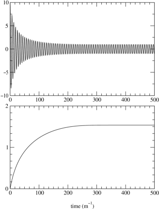
FIG. 1.: Evolution of the scalar field amplitude and scale factor for $mr_{0}=1000$ and $r^{2}_{0}\mu^{2}=50$.

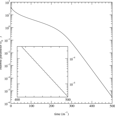
FIG. 2.: Evolution of the Hubble parameter for the example shown in Figure 1. The inset highlights the details in the evolution that result from the oscillating field.

This asymptotic dynamics is generic for systems with a negative cosmological constant and matter on a braneworld. As another example of a system that has these elements, consider a scalar field, $\phi$, living exclusively on the brane with the potential One can envision that this scalar field may be an inflaton, quintessence or other such cosmological field. The constant offset acts as a negative cosmological constant, with $\lambda=-m^{2}\phi_{0}^{2}/2$. Fluctuations in the field around the true vacuum state act as the matter. A more general potential may always be considered, but this example captures the qualitative features of interest. Consider the brane homogeneously filled with a scalar field possessing such a potential. The equations describing the scalar field evolutions is

$$\ddot{\phi}+3H\dot{\phi}+m^{2}\phi=0\ ,$$ (31)

and the Hubble parameter is determined by Eq. (24) when

$$\rho_{b}={1\over 2}\dot{\phi}^{2}+V(\phi)\ .$$ (32)

Once again, the precise evolution of the system is dependent on two parameters: the crossover scale, $r_{0}$, and the quantity $r^{2}_{0}\mu^{2}$, and the qualitative features are the same. Figures 1 and 2 depict the evolution of the scalar field, the scale factor, and the Hubble parameter of a typical case. With a positive energy density, the field oscillates with a damping proportional to the Hubble parameter. Eventually, the energy density is drawn toward zero, and the scalar field exponentially asymptotes to a dissipationless oscillation.

One expects that the oscillations in the scalar field amplify spatially inhomogeneous perturbations in that field. However, if the self-coupling of that field is small, such an amplification does not grow without bound. Also, unlike the matter considered earlier, the asymptotic metric of the spacetime is not static. Although the energy density vanishes, the pressure is a rapidly oscillating function.

III Global structure of spacetime

As shown explicitly in [6, 19] (see also[20]) the bulk spacetime in Eq. (9) is two identical pieces of 5-dimensional Minkowski spacetime glued across the braneworld worldvolume. The same holds true for the asymptotic solution, Eq. (6), where the bulk is now a piece of Rindler spacetime. In this latter case the $y={\rm constant}$ surfaces in the $(\tau,y)$ plane are hyperbolas ${\cal H}_{y}$ in the two dimensional Minkowski space time, so that the brane space-time (6) is the hyperbolic cylinder $\cal C$ defined by ${\cal H}_{0}\times E_{3}$, where $E_{3}$ is the 3 dimensional Euclidian plane. The whole spacetime reflected in Eq. (6) is then simply given by gluing two copies of one side of ${\cal C}$ along ${\cal C}$.

This picture of the global structure of spacetime may be verified explicitly using a new set of coordinates $Y^{A}$ ($A=0,1,2,3,5$) of 5-dimensional Minkowski spacetime. The line element may be written

$$ds^{2}=-(dY^{0})^{2}+(dY^{1})^{2}+(dY^{2})^{2}+(dY^{3})^{2}+(dY^{5})^{2}\ ,$$ (33)

where the coordinate change need to arrive at this line element is determined by equations given in [6, 19].

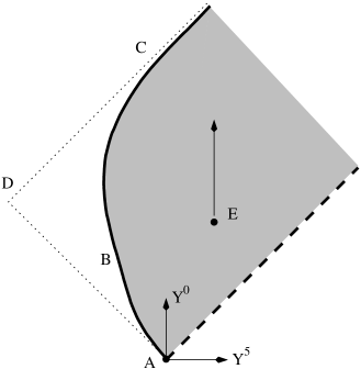
FIG. 3.: Global Minkowski space for a specific spatial slice. The shaded region represents the bulk spacetime and the solid line represents the boundary braneworld worldline on which two identical bulks are glued together. (A) For conventional matter content, the braneworld originates at a big bang singularity which evolves in a lightlike direction. (B) The evolution of the braneworld depends on the specific matter content. (C) Eventually, the braneworld asymptotes to a future Rindler horizon and to the static solution. Equal braneworld time curves approximately radiate outwards from the light cone origin at point (D). Note that a bulk observer (E) is always attracted to the braneworld and eventually encounters it. This picture is consistent with the braneworld point of view that suggests that bulk observers are attracted to the braneworld from a warp factor that increases as one goes out into the bulk.

We are mainly interested in the coordinate change for late times when the braneworld system approaches a static state. In this case, whether one considers an intrinsic curvature term Eq. (2) or not, we may use the solution in Eq. (20) for the scale factor. Equation (20) may be rewritten as

$$a=a_{\infty}(1-\epsilon)^{1/q}\ ,$$ (34)

with $a_{\infty}$ a constant given by

$$a_{\infty}=\left(-\frac{\rho_{0}}{\lambda}\right)^{1/q}$$ (35)

is the $t\rightarrow\infty$ limit of the scale factor if $a(t=t_{0})=1$. The quantity $\epsilon$ defined by

$$\epsilon\equiv\left(1+\frac{\lambda}{\rho_{0}}\right)e^{-(t-t_{0})/T}\ ,$$ (36)

which is small for asymptotically late times, and where the time scale $T$ is given by

$$T\equiv-6M_{(5)}^{3}/\lambda q\ .$$ (37)

Using the formulas given in [19], one finds at leading order in $\epsilon$

$$Y^{0}+Y^{5}-\frac{a_{\infty}r^{2}}{2} = \epsilon^{-1}\frac{qT^{2}}{2a_{\infty}}\left(1+\frac{|y|}{T}\right),$$ (38)

$$Y^{0}-Y^{5}-2a_{\infty} = -\epsilon\frac{2a_{\infty}}{q}\left(1+\frac{|y|}{T}\right),$$ (39)

$$Y^{i} = a_{\infty}x^{i}\ ,$$ (40)

where $r=x^{i}x_{i}$. One then easily sees that up to terms of order $\epsilon$ (and a change in the origin of the Y-coordinate system), one has for a given $r={\rm constant}$ slice

$${(Y^{0})}^{2}-{(Y^{5})}^{2}=-T^{2}\left(1+\frac{|y|}{T}\right)^{2}\ .$$ (41)

For asymptotically late times, the world line of the braneworld follows this hyperbola. At specific time slices, the braneworld coordinates, $Y^{0}$ and $Y^{5}$ evolve toward infinity asymptoting the light cone, and the values of those coordinates grow exponentially with cosmological (braneworld) time $t$. Figure 3 depicts the global 5-dimensional Minkowski space for a given spatial slice.

IV Four-dimensional gravity

A Propagator on the brane

We can now study the propagation of gravitons in this asymptotic static space. The line element reads as follows:

$$ds^{2}~{}=~{}-\left(1+r_{0}\mu^{2}|y|\right)^{2}d\tau^{2}~{}+~{}dx_{i}dx^{i}~{}+~{}dy^{2}~{}\ .$$ (42)

For simplicity we treat the graviton as a scalar particle. As was emphasized in [4, 21], the scalar part of the graviton propagator reduces to that of a minimally coupled spin-0 particle in various backgrounds which we study below.

Let us start with the action:

$$\int~{}d^{4}x~{}dy\left(~{}{M^{3}_{(5)}\over 2}\sqrt{{\tilde{g}}}~{}{\tilde{g}}^{AB}\partial_{A}\phi~{}\partial_{B}\phi~{}+~{}{M^{2}_{(4)}\over 2}~{}\delta(y)~{}\sqrt{{g}}~{}{g}^{ab}\partial_{a}\phi~{}\partial_{b}\phi~{}\right)~{}.$$ (43)

The first term here is a counterpart of the bulk Einstein action and the second one accounts for the induced curvature term. The equation for the Green function takes the form:

$$\left({M^{3}_{(5)}}~{}\partial_{A}\sqrt{{\tilde{g}}}\partial^{A}~{}+~{}\delta(y){M^{2}_{(4)}}~{}\partial_{b}\sqrt{{g}}\partial^{b}\right)G(x_{a},y)~{}=~{}M^{3}_{(5)}\sqrt{g}\delta^{(4)}(x)\delta(y)~{}.$$ (44)

Using (42) we find:

$$\left\{-{1\over(1+r_{0}\mu^{2}|y|)}\partial_{\tau}^{2}~{}+~{}(1+r_{0}\mu^{2}|y|)\partial_{i}^{2}~{}+~{}\partial_{y}(1+r_{0}\mu^{2}|y|)\partial_{y}\right\}~{}G(x_{a},y)~{} +$$ (45)

$$2r_{0}\delta(y)\left\{-{1\over(1+r_{0}\mu^{2}|y|)}\partial_{\tau}^{2}~{}+~{}(1+r_{0}\mu^{2}|y|)\partial_{i}^{2}~{}\right\}G(x_{a},y) = \delta^{(4)}(x)\delta(y)~{}.$$ (46)

To find the Green’s function it is convenient to perform Fourier transform to momentum space with respect to the four worldvolume coordinates $x_{a}$,

$$G(\tau,x_{i},y)~{}\equiv~{}\int{d\omega~{}d{\bf q}_{i}\over(2\pi)^{4}}e^{i\omega\tau}e^{-i{\bf q}\cdot{\bf x}}~{}{\tilde{G}}(\omega,{\bf q}_{i},y)~{}.$$ (47)

As a result, the equation takes the form:

$$\left\{{\omega^{2}\over(1+r_{0}\mu^{2}|y|)}~{}-~{}(1+r_{0}\mu^{2}|y|){\bf q}_{i}^{2}~{}+~{}\partial_{y}(1+r_{0}\mu^{2}|y|)\partial_{y}\right\}~{}{\tilde{G}}(\omega,q,y) +$$ (48)

$$2r_{0}\delta(y)\left\{\omega^{2}~{}-~{}{\bf q}_{i}^{2}~{}\right\}{\tilde{G}}(\omega,q,y) = \delta(y)~{}.$$ (49)

Let us introduce the following notation:

$${\tilde{G}}~{}\equiv~{}{1\over\sqrt{1+r_{0}\mu^{2}|y|}}\chi~{}.$$ (50)

Making use of this relation, the resulting equation reads as follows:

$$\chi^{\prime\prime}~{}+~{}\left[{\omega^{2}~{}+~{}(r_{0}\mu^{2})^{2}/4\over(1+r_{0}\mu^{2}|y|)^{2}}-{\bf q}_{i}^{2}\right]~{}\chi~{}+~{}2r_{0}\delta(y)\left\{\omega^{2}~{}-~{}{\bf q}_{i}^{2}~{}\right\}~{}\chi~{}=~{}\delta(y)\left[1+r_{0}\mu^{2}\chi(0)\right]~{}.$$ (51)

To find the solution of this equation with appropriate boundary conditions let us introduce the following substitution:

$$\chi(\omega,{\bf q}_{i},y)~{}=~{}B(\omega,{\bf q}_{i})~{}\Sigma(y)~{},$$ (52)

where $\Sigma$ satisfies the following equation:

$$\Sigma^{\prime\prime}~{}+~{}\left[{\omega^{2}~{}+~{}(r_{0}\mu^{2})^{2}/4\over(1+r_{0}\mu^{2}|y|)^{2}}-{\bf q}_{i}^{2}\right]~{}\Sigma~{}=~{}\delta(y)~{}.$$ (53)

From this definition, as well as from Eq. (52), one sees that the expression for the Green’s function on the brane ($y=0$) takes the form:

$${\tilde{G}}|_{y=0}~{}=~{}~{}\left[-2r_{0}q^{2}-r_{0}\mu^{2}+\Sigma(0)^{-1}\right]^{-1}\ ,$$ (54)

where we have defined $q^{2}=-\omega^{2}+{\bf q}_{i}^{2}$, the invariant 4-momentum squared.

The solution to Eq. (53) with asymptotically vanishing behavior as $|y|\rightarrow\infty$ is [22]

$$\Sigma(y)\sim\sqrt{u}K_{\nu}(u/2)\ ,$$ (55)

with

$$u=\frac{1+r_{0}\mu^{2}|y|}{r_{0}\mu^{2}}2|{\bf q}_{i}|\ ,$$ (56)

and $K_{\nu}$ is the MacDonald function of order $\nu=\pm i\omega/r_{0}\mu^{2}$. The normalization of $\Sigma(y)$ may be established by the delta function in the right-hand side of Eq. (53), indicating that

$$\Sigma^{\prime}(y=0^{+})=\frac{1}{2}\ .$$ (57)

One obtains

$$\Sigma(0)^{-1}=2|{\bf q}_{i}|\left[\frac{1-2\nu}{u_{0}}-\frac{K_{\nu-1}(u_{0}/2)}{K_{\nu}(u_{0}/2)}\right]\ ,$$ (58)

where we define

$$u_{0}\equiv u(y=0)=\frac{2|{\bf q}_{i}|}{r_{0}\mu^{2}}\ .$$ (59)

Using Eq. (54), one finds the exact expression of the propagator on the brane:

$${\tilde{G}}|_{y=0}~{}=~{}~{}\frac{1}{2r_{0}}\left[-q^{2}\mp\frac{i\omega}{r_{0}}-\frac{|{\bf q}_{i}|}{r_{0}}\frac{K_{-1\pm i\omega/r_{0}\mu^{2}}\left(|{\bf q}_{i}|/r_{0}\mu^{2}\right)}{K_{\pm i\omega/r_{0}\mu^{2}}\left(|{\bf q}_{i}|/r_{0}\mu^{2}\right)}\right]^{-1}\ .$$ (60)

In the above expression the first term on the right hand side represents the usual 4-dimensional Lorentz invariant propagator, whereas the two other terms are responsible for deviation from 4-dimensional behavior as well as for Lorentz violating effects.

B Asymptotic developments

We wish to elaborate on the propagator Eq. (60) in some special limits. We see that the propagator is 4-dimensional Lorentz symmetry violating in general. Let us first examine the limit in which the spatial momentum ${\bf q}_{i}\rightarrow 0$, with $\omega\neq 0$. Taking the propagator with outgoing radiative boundary conditions, at leading order

$${\tilde{G}}|_{y=0}^{-1}~{}=~{}2r_{0}\omega^{2}-2i\omega\ .$$ (61)

We see then a restoration of the propagator found in [4] in the same limit, indicating there is no massive graviton state stationary with respect to the cosmological frame.

Next we wish to take the limit where the propagator yields the static potential, $\omega\rightarrow 0$.

$${\tilde{G}}|_{y=0}^{-1}~{}=~{}-2r_{0}{\bf q}_{i}^{2}-2|{\bf q}_{i}\frac{K_{1}(|{\bf q}_{i}|/r_{0}\mu^{2})}{K_{0}(|{\bf q}_{i}|/r_{0}\mu^{2})}\ .$$ (62)

Note that this form is not covariant with respect to the form found in Eq. (61). For large distances ($|{\bf q}_{i}|\rightarrow 0$), the propagator reduces to

$${\tilde{G}}|_{y=0}~{}=~{}\frac{1}{2r_{0}\mu^{2}}\ln\frac{|{\bf q}_{i}|}{2r_{0}\mu^{2}}\ .$$ (63)

This form corresponds to a $r^{-3}$ static potential. For short distances, ($|{\bf q}_{i}|\rightarrow\infty$), the propagator reduces to

$${\tilde{G}}|_{y=0}~{}=~{}-\frac{1}{2r_{0}{\bf q}_{i}^{2}}\ ,$$ (64)

corresponding to a $r^{-1}$ static potential. Crossover behavior varies depending on the value of the dimensionless parameter, $r_{0}\mu$.

In order to see the restoration of 4-dimensional Lorentz invariance, we must go to large values of $\omega$ and ${\bf q}_{i}$. Taking $r_{0}\mu^{2}\rightarrow 0$ while holding $\omega$ and ${\bf q}_{i}$ fixed, the propagator becomes

$${\tilde{G}}|_{y=0}^{-1}~{}=~{}-2r_{0}q^{2}-2q-r_{0}\mu^{2}(1+\omega^{2}/q^{2})\ .$$ (65)

Note that when $r_{0}\mu^{2}\rightarrow 0$, explicit 4-dimensional Lorentz invariance is recovered and the propagator reduces to the form found in [4]. Equation (65) expresses the dominant off-shell behavior for the scalar graviton propagator.

Alternatively, when $q^{2}\rightarrow 0$, but in a manner such that $\omega^{2}\gg r_{0}^{2}\mu^{4}$ with $q/\omega<(r_{0}\mu^{2}/\omega)^{1/3}$, then

$${\tilde{G}}|_{y=0}^{-1}~{}=~{}-2r_{0}q^{2}-2\omega~{}\frac{\Gamma(2/3)}{\Gamma(1/3)}\left({6r_{0}\mu^{2}\over\omega}\right)^{1/3}\ .$$ (66)

The pole in the propagator in this regime indicates the following dispersion relationship for an on-shell particle:

$$\omega^{2}={\bf q}_{i}^{2}+\frac{\Gamma(2/3)}{\Gamma(1/3)}\left(6r_{0}\mu^{2}\right)^{1/3}({\bf q}_{i}^{2})^{1/3}\ .$$ (67)

As $|{\bf q}_{i}|\rightarrow\infty$, the first term in the expression is dominant and the expected relativistic dispersion relationship is recovered.

V Concluding Remarks

Our system has the property of having energy density evolve to zero from a generic set of initial conditions with positive energy density. The pressure of this asymptotic state is non-zero, so the full 5-dimensional spacetime explicitly breaks 4-dimensional Lorentz invariance, even while the induced metric on the braneworld is Minkowskian. The graviton propagator on such a braneworld also reflects a lack of 4-dimensional Lorentz symmetry, since that graviton can probe the full spacetime.

A static Minkowski braneworld coupled to a braneworld energy-momentum which explicitly violates 4-dimensional Lorentz symmetry is possible because the larger metric of the 5-dimensional space does not respect 4-dimensional Lorentz symmetry. Any slice of the 5-dimensional spacetime parallel to the braneworld is indeed Minkowski. However, the speed of light varies from slice to slice. If standard model particles trapped on the braneworld do not couple to the dark matter generating the 5-dimensional spacetime, then there should be no observable Lorentz symmetry violation in the standard model, except through graviton exchange.

One can ask how well this model complies with known phenomenology. We have two parameters that may be adjusted: the crossover scale, $r_{0}=M^{2}_{(4)}/2M^{3}_{(5)}$, which reflects the relative sizes of the 4-dimensional Planck mass and the 5-dimensional Planck mass, as well as $\mu^{2}=-\lambda/M^{2}_{(4)}$, which reflects the relative size of the brane cosmological constant to the 4-dimensional Planck scale.

We may place constraints on the system parameters at various stages. Let us first address solely the constraints from gravitational force law observations. The exchange of the tower of Kaluza-Klein (KK) modes may be understood from the 4-dimensional point of view as an exchange of a metastable graviton [3, 23, 1]. The decay width is controlled by the larger of the two energy scales $r_{0}^{-1}$ or $\mu$. Thus, both energy scales must be tuned to some sufficiently small value to be consistent with a stable, massless graviton. We know that the graviton is stable and massless up until $\sim 100$ parsecs (for a discussion, see [24]). We may choose the galactic size as well, but for here we settle for a strict confirmation of the $1/r^{2}$ force law. Then both $r_{0}$, and $\mu^{-1}$ must be as large as $100$ parsecs. This places constraints on $M_{(5)}<100\ {\rm GeV}$ and $|\lambda|<(10\ {\rm eV})^{4}$.

We may also constrain our system parameters based on the standard cosmological model. We found that early cosmology only follows the conventional hot big bang scenario when the energy density on the brane is much larger than $|\lambda|$ as well as a similar constraint between the Hubble parameter and the crossover scale $r_{0}^{-1}$. Cosmology constraints imply $M_{(5)}<100\ {\rm MeV}$ and $|\lambda|<(10^{-3}\ {\rm eV})^{4}$.

Having such a small fundamental Planck scale, $M_{(5)}$, does not contradict any astrophysical or particle physics bounds as long as there is a 4-dimensional induced Planck scale on the brane (see [7]), assuming quantum gravity becomes soft above this energy scale. However, in the present context this issue deserves clarification, due to the presence of a Lorentz symmetry violating metric which is not considered in [7]. Since the Lorentz violation is due to a tiny cosmological constant, the prior analysis should be valid, and any new effect should be a small perturbation. On the other hand, the warp factor (which parametrizes Lorentz symmetry violation) diverges as $M_{(5)}\rightarrow 0$. While this statement is true, Lorentz symmetry violation in the propagator on the brane is controlled by the second and thirds terms on the right-hand side of Eq. (60). For small $M_{(5)}$ (when $M_{(4)}$ and $\lambda$ are fixed) those terms are suppressed relative to the leading 4-dimensional contribution to the propagator. In other words, although the Lorentz violating warp factor becomes steep when $M_{(5)}$ is small, it cannot strongly affect brane observers since probing the bulk becomes more difficult. This can be also understood in the KK-mode expansion. In this language, the intrinsic curvature term repels KK-modes heavier than $1/r_{0}$, suppressing their wavefunction on the brane and shielding the brane from bulk gravity effects, in particular Lorentz symmetry violation.

All these observations imply that one cannot start with a large cosmological constant on the brane, and therefore this model cannot yield a resolution of the cosmological constant problem. The mechanism that so generously compels the total energy density to zero is equally unforgiving. Any combination of matter whose total energy density is on the order of magnitude of the cosmological constant evolves exponentially fast to a flat and perfectly static universe, in a time comparable to $M^{3}_{(5)}/|\lambda|$.

We have proposed a model which has some intriguing properties. It dynamically evolves to a zero energy-density state and provides a novel mechanism for producing a static, Lorentz symmetry violating universe. Perhaps these mechanisms may be applied to more phenomenologically promising models in the future.

- [1] G. Dvali, G. Gabadadze and M. Porrati, Phys. Lett. B 484, 112 (2000).
- [2] E. Witten, hep-ph/0002297.
- [3] R. Gregory, V. A. Rubakov and S. M. Sibiryakov, Phys. Rev. Lett. 84, 5928 (2000).
- [4] G. Dvali, G. Gabadadze and M. Porrati, Phys. Lett. B 485, 208 (2000).
- [5] G. Dvali and G. Gabadadze, Phys. Rev. D 63, 065007 (2001).
- [6] C. Deffayet, Phys. Lett. B 502, 199 (2001).
- [7] G. Dvali, G. Gabadadze, M. Kolanović and F. Nitti, hep-ph/0102216.
- [8] L. Gonzalez-Mestres, hep-ph/9610474.
- [9] S. Coleman and S. L. Glashow, Phys. Lett. B 405, 249 (1997), Phys. Rev. D 59, 116008 (1999).
- [10] M. Visser, Phys. Lett. B 159, 22 (1985).
- [11] G. Dvali and M. Shifman, Phys. Rept. 320, 107 (1999).
- [12] C. Csáki, J. Erlich, and C. Grojean, hep-th/0012143.
- [13] S. L. Dubovsky, hep-th/0103205.
- [14] P. Kraus, JHEP9912, 011 (1999).
- [15] P. Binétruy, C. Deffayet and D. Langlois, Nucl. Phys. B 565, 269 (2000).
- [16] T. Shiromizu, K. Maeda and M. Sasaki, Phys. Rev. D 62, 024012 (2000).
- [17] E. E. Flanagan, S. H. Tye and I. Wasserman, Phys. Rev. D 62, 044039 (2000).
- [18] P. Binétruy, C. Deffayet, U. Ellwanger and D. Langlois, Phys. Lett. B 477, 285 (2000).
- [19] N. Deruelle and T. Dolezel, Phys. Rev. D 62, 103502 (2000).
- [20] S. Mukohyama, T. Shiromizu and K. Maeda, Phys. Rev. D 62, 024028 (2000) [Erratum-ibid. D 63, 024028 (2000)].
- [21] B. Bajc and G. Gabadadze, Phys. Lett. B 474, 282 (2000).
- [22] G. N. Watson, Theory of Bessel Functions, Cambridge University Press, 1922.
- [23] C. Csaki, J. Erlich and T. J. Hollowood, Phys. Rev. Lett. 84, 5932 (2000); C. Csaki, J. Erlich, T. J. Hollowood, and J. Terning, Phys. Rev. D 63 065019 (2001).
- [24] C. M. Will, Phys. Rev. D 57, 2061 (1998).