Late-Time Evolution of Charged Massless Scalar Field in the Spacetime of Dilaton Black Hole

Abstract

We investigate the power-law tails in the evolution of a charged massless scalar field around a fixed background of dilaton black hole. Using both analytical and numerical methods we find the inverse power-law relaxation of charged fields at future timelike infinity, future null infinity and along the outer horizon of the considered black hole. We invisaged that a charged hair decayed slower than neutral ones. The oscillatory inverse power-law along the outer horizon of dilaton black hole is of a great importance for a mass inflation scenario along the Cauchy horizon of a dynamically formed dilaton black hole.

I Introduction

The late-time evolution of various fields outside a collapsing star plays an important role in major aspects of black hole physics, i.e., in the Wheeler’s no-hair theorem [1] and in mass inflation scenario [2]. In Ref.[3] the neutral external perturbations were studied and it was found that the late-time behaviour for a fixed $r$ is dominated by the factor $t^{-(2l+3)}$, for each multipole moment $l$. Next, Gundlach et al [4] studied the behaviour of neutral perturbations along null infinity and along future event horizon. Their conclusion was that along null infinity the decay is according the power law of the form $u^{-(l+2)}$, where $u$ is the outgoing Eddington-Filkenstein (ED) null coordinate. On the other hand, the neutral perturbations along the event horizon behave like $v^{-(l+3)}$, where $v$ is the ingoing ED coordinate. Bicak [5] analysed the scalar field perturbations on Reissner-Nordström (RN) background and found for $\mid Q\mid<M$ the relation $t^{-(2l+2)}$, while for $\mid Q\mid=M$ the late-time behaviour for a fixed $r$ was governed by the rule $t^{-(l+2)}$.

The late-time behaviours of a charged massless scalar field in RN spacetime were studied analytically and confirmed by the direct numerical studies of the fully nonlinear gravitational collapse in [6, 7, 8]. Among all, the conclusion was that a charged hair decayed slower than a neutral one, i.e., the charged scalar hair outside a charged black hole was dominated by a $t^{-(2l+2)}$ behaviour.

The problem of the late-time tails in gravitational collapse of a self interacting massive field were studied in [9] (see also [10, 11, 12]). At late-times the decays of a self-interacting hair is slower than any power law.

In our work we shall discuss the asymptotic evolution of a massless charged scalar field in the background of dilaton black hole. Focusing on no-hair theorem we shall be interested in the dynamical mechanism by which the charged hair is radiated away. In Sec.II we start with the outline of the system under consideration and we analitycally study the late-time evolution of charged scalar perturbations along timelike infinity, future null infinity and the black hole outer horizon. Then, in Sec.III we treated the problem numerically. Sec.IV outlines our conclusions and remarks.

II The Einstein-Maxwell-dilaton Equations

In this section we shall analytically study the evolution of a massless charged scalar field $\psi$ around a fixed background of electrically charged dilaton black hole. The wave Eq. for a massless charged scalar field is given by [13]

$$\nabla_{\mu}\nabla^{\mu}\psi-ieA_{\alpha}g^{\alpha\beta}(2\nabla_{\beta}\psi-ieA_{\beta}\psi)-ie\nabla_{\mu}A^{\mu}\psi=0,$$ (1)

where $e$ is a constant value and $A_{\beta}$ is the gauge potential.

The metric of the external gravitational field will be given by the static, spherically symmetric solution of Eqs. of motion derived from the low-energy string action (see e.g.[14]). The action has the form as follows:

$$S=\int d^{4}x\left[R-2(\nabla\phi)^{2}-e^{-2\phi}F^{2}\right],$$ (2)

where $\phi$ is the dilatonic field and $F_{\alpha\beta}=2\nabla_{[\alpha}A_{\beta]}$. The metric of the electrically charged dilaton black hole is as follows:

$$ds^{2}=-\left(1-{2M\over r}\right)dt^{2}+{dr^{2}\over\left(1-{2M\over r}\right)}+r\left(r-{Q^{2}\over M}\right)(d\theta^{2}+\sin\theta d\phi^{2}).$$ (3)

The event horizon is located at $r_{+}=2M$. For the case of $r_{-}={Q^{2}\over M}$ we have another singularity but it can be ignored because of the fact that $r_{-}<r_{+}$. The dilaton field is given by $e^{2\phi}=e^{-2\phi_{0}}\left(1-{r_{-}\over r}\right)$, where $\phi_{0}$ is the dilaton’s value at $r\rightarrow\infty$. The mass $M$ and the charge $Q$ are related by the relation $Q^{2}={r_{+}r_{-}\over 2}e^{2\phi_{0}}$.
Defining the tortoise coordinate $y$, as $dy={dr\over\left(1-{2M\over r}\right)}$ one can rewrite the metric (3) in the form

$$ds^{2}=\left(1-{2M\over r}\right)\left[-dt^{2}+dy^{2}\right]+r\left(r-{Q^{2}\over M}\right)(d\theta^{2}+\sin\theta d\phi^{2}).$$ (4)

For the spherical background each of the multipole of perturbation field evolves separetly so for the scalar field in the form $\psi=\sum_{l,m}\eta_{m}^{l}(t,r)Y_{l}^{m}(\theta,\phi)/R(r)$, one has the following Eqs. of motion for each multipole moment

$$\eta_{,tt}-2ieA_{t}\eta_{,t}-\eta_{,yy}+V\eta=0,$$ (5)

where

$$V=\left[{l(l+1)\over R^{2}}+{R^{\prime\prime}\over R}\left(1-{2M\over r}\right)+{2MR^{\prime}\over r^{2}R}\right]\left(1-{2M\over r}\right)-e^{2}A_{t}^{2}.$$ (6)

By $R$ we denoted $R=\sqrt{r\left(r-{Q^{2}\over M}\right)}$ and ^′ is the derivative with respect to the $r$-coordinate. As in Ref.[6] in order to get rid of the physically unimportant quantity $\tilde{\Phi}$, which appear in $A_{t}=\tilde{\Phi}-{Q\over r}$, one can define the auxilary field $\tilde{\psi}=e^{-ie\tilde{\Phi}t}\eta$. Then Eq.(5) may be written as

$$\tilde{\psi}_{,tt}+2ie{Q\over r}\tilde{\psi}_{,t}-\tilde{\psi}_{,yy}+{\tilde{V}}\tilde{\psi}=0,$$ (7)

where

$${\tilde{V}}=\left[{l(l+1)\over R^{2}}+{R^{\prime\prime}\over R}\left(1-{2M\over r}\right)+{2MR^{\prime}\over r^{2}R}\right]\left(1-{2M\over r}\right)-{e^{2}Q^{2}\over r^{2}}.$$ (8)

One can assume that the general solution of Eq.(7) is of the form

$$\tilde{\psi} = \sum_{k=0}^{l}A_{k}R^{-k}\left[e^{-ieQlnr}G(u)^{(l-k)}+(-1)^{k}e^{ieQlnr}F(v)^{(l-k)}\right]$$ (9)

$$+ \sum_{k=0}^{\infty}\left[B_{k}(R)G(u)^{(l-k-1)}+C_{k}F(u)^{(l-k-1)}\right],$$ (10)

where $F$ and $G$ are arbitrary functions of an retarded time coordinate $u=t-y$ and an advanced time coordinate $v=t+y$. The superindices on $F$ and $G$ have different meaning depending on negativity or positivity of them. The positive superindices indicate the number of times the function is differentiated, while the negative ones are to be interpreted as integrals [3]. The first sum in $\tilde{\psi}$ represents the primary waves in the wavefront while the second sum depicts the backscattered waves. The first sum in the above expression is the zeroth order solution.
The recursion relation for $B_{k}(R)$ is as follows:

$$2{\lambda}^{2}B_{k}(R)^{\prime} + {2ieQ\over r}B_{k}(R)-{\lambda}^{2}\left[{\lambda}^{2}B_{k-1}(R)^{\prime}\right]^{\prime}+{\lambda}^{2}\left[A_{k}(R)(kR^{\prime}+ieQ){1\over R^{k+1}r^{ieQ}}\right]^{\prime}$$ (11)

$$+ {\tilde{V}}\left[A_{k}(R)R^{-k}r^{-ieQ}+B_{k-1}(R)\right]+2A_{k+1}(R){\left[ieQ(R-r{\lambda}^{2})-{\lambda}^{2}rR^{\prime}(k+1)\right]\over R^{k+1}r^{ieQ+1}}=0,$$ (12)

where ${\lambda}=\left(1-{2M\over r}\right)$. We expand the $B_{k}(R)$ coefficient in the form

$$B_{k}(R)={a_{k}\over R^{k+1}r^{ieQ}}+{b_{k}\over R^{k+1}r^{ieQ+1}}+...,$$ (13)

where as in [3] $a_{k}=a_{k}(l,eQ)$, $b_{k}=b_{k}(l,eQ)$.
Using Eqs.(11) and (13) the lowest order coefficients yield

$$a_{k}=-ieQA_{k}(R){2k+1\over 2(k+1)}\left[1+{\cal O}(eQ)\right].$$ (14)

As was pointed out after starting of collapsing of the star surface it approached very fast the speed of light. Thus its word line is asymptotic to an ingoing null geodesics $v=v_{0}$. The time dilatation between static frames and infalling frames caused that the variation of the field $\tilde{\psi}$ on the star’s surface is asymptotically redshifted. This means that $\tilde{\psi}_{,u}$ will be small at late times. Then it is well justified to make an assumption that after some retarded time $u=u_{1}$ variations of the charged field $\tilde{\psi}$ on $v=v_{0}$ can be neglected.
In the first stage of evolution we shall consider the scattering in the region $u_{0}<u<u_{1}$. One has taken the variation of the field on $v=v_{0}$ to be neglected after $u_{1}$. Thus, we have no outgoing radiation for $u>u_{1}$, except from backscattering. This assumption about no late outgoing waves is equivalent to taking $G(u_{1})=0$. Summing it all up, for large $r$ at $u=u_{1}$ the dominant term in $\tilde{\psi}$ (the dominant backscatter of the primary waves) is as follows:

$$\tilde{\psi}(u=u_{1},r)=a_{l}{1\over r^{l+1}}G^{(-1)}(u_{1}).$$ (15)

In the next stage of the consideration we take a closer look at the asymptotic evolution of the charged scalar field. We shall take into consideration the region where $y\gg M,Q$ and for which $u>u_{1}$. In this region the leading order effect on the propagation of $\tilde{\psi}$, has the centrifugal term in the potential ${\tilde{V}}$, namely the evolution is dominated by a neutral flat spacetime terms. Thus one has

$$\tilde{\psi}_{,tt}-\tilde{\psi}_{,rr}+{l(l+1)\over r^{2}}\tilde{\psi}=0.$$ (16)

As in RN case in this region one can replace $r$ by $y$, because of the fact that $\tilde{\psi}_{,yy}\simeq\tilde{\psi}_{,rr}+{\cal O}(M)$. The solution to Eq.(16) can be written in the form

$$\tilde{\psi}=\sum_{l=0}^{k}A_{k}y^{-k}\left[g^{(l-k)}(u)+(-1)^{k}f^{(l-k)}(v)\right].$$ (17)

Matching (17) with initial data on $u=u_{1}$ Eq.(15), one has $f(v)=F_{0}v^{-1}$, where $F_{0}$ is of the same form as in RN case [6]. The standard procedure of expansion [3], for late times $t\gg y$ for $g(u)=\sum_{n=0}^{\infty}{(-1)^{n}\over n!}g^{(n)}(t)y^{n}$ and similary $f(v)=\sum_{n=0}^{\infty}{1\over n!}f^{(n)}(t)y^{n}$, enables one to rewrite (17) as follows:

$$\tilde{\psi}=\sum_{n=-1}^{\infty}K_{n}y^{n}\left[f^{(l+n)}(t)+(-1)^{n}g^{(l+n)}(t)\right],$$ (18)

where $K_{n}$ are given in Ref.[3] as in the neutral case.
Using the boundary conditions for small $r$ (see [3] and [4] for the details), one finds that the late time behaviour of the scalar field at timelike infinity $i_{+}$ is

$$\tilde{\psi}\simeq 2K_{l+1}y^{l+1}f^{(2l+1)}(t)=-2K_{l+1}F_{0}(2l+1)!t^{-2(l+1)}y^{l+1}+{\cal O}(eQ).$$ (19)

On a future null infinity $scri_{+}$ one has

$$\tilde{\psi}(v\gg u,u)\simeq A_{0}g^{(l)}(u)\simeq-F_{0}l!u^{-(l+1)}.$$ (20)

At the black hole outer horizon $H_{+}$ (as $y\rightarrow-\infty$) the Eq. of motion can be approximated by

$$\tilde{\psi}_{,tt}+{ieQ\over M}\tilde{\psi}_{,t}-\tilde{\psi}_{,yy}-{e^{2}Q^{2}\over 4M^{2}}\tilde{\psi}=0,$$ (21)

with the general solution of the form

$$\tilde{\psi}=e^{-{ieQ\over 2M}t}\left[\alpha(u)+\gamma(v)\right]=e^{-{ieQ\over 2M}t}\gamma(v).$$ (22)

We put $\alpha(u)=0$ because of the condition of neglecting the variation of the scalar field on $v=v_{0}$. To join the solution for $y\ll-M$ with $y\gg M$ for $i_{+}$, one uses the ansatz [4, 6] $\tilde{\psi}\simeq\tilde{\psi}_{stat}t^{-2(l+1)}$ for the solution in region $y\ll-M$ and $t\gg\mid y\mid$, i.e., we assume that for the whole range of $y$ the solution has the same late-time dependence as for $y\gg M$. This enables us to match the solution (22) with that for $i_{+}$. One concludes that the late-time behaviour on the horizon $H_{+}$ is

$$\tilde{\psi}(u\rightarrow\infty,v)=\Gamma_{0}e^{ieQy\over 2M}v^{-2(l+1)},$$ (23)

where the constant $\Gamma_{0}$ is detrmined by the condition that there is a static solution fulfilling $lim_{y\rightarrow\infty}\tilde{\psi}_{finstat}=\Gamma_{0}$ and $lim_{y\rightarrow\infty}\tilde{\psi}_{finstat}=-2K_{l}^{2l+1}F_{0}(1+2l)!r^{l+1}$. As was remarked in [3, 4], the coefficient $\Gamma_{0}$ and all other aspects of the late-time behaviour are governed by the initial backscattering.
As one can see the behaviour of the charged scalar field on a fixed dilatonic background at timelike null infinity $i_{+}$ and the future null infinity $scri_{+}$ is the same as in the RN black hole case. However, on the external horizon $H_{+}$ we have some changes, but the general form of the time dependence is maintained.

III Numerical method and results

In this section we shall numerically study Eqs.(7) and (8). First we transform Eq.(7) into $(u,v)$ coordinates. This yields:

$$4\tilde{\psi}_{,uv}+2ie{Q\over r}(\tilde{\psi}_{,u}+\tilde{\psi}_{,v})+{\tilde{V}}\tilde{\psi}=0.$$ (24)

Then we divide this Eq. into a set of coupled equations for real, $\tilde{\psi}_{\rm R}$, and imaginary, $\tilde{\psi}_{\rm I}$, parts of the field.

$$4\tilde{\psi}_{{\rm R},uv}-2e{Q\over r}(\tilde{\psi}_{{\rm I},u}+\tilde{\psi}_{{\rm I},v})+{\tilde{V}}\tilde{\psi}_{\rm R}=0.$$ (25)

$$4\tilde{\psi}_{{\rm I},uv}+2e{Q\over r}(\tilde{\psi}_{{\rm R},u}+\tilde{\psi}_{{\rm R},v})+{\tilde{V}}\tilde{\psi}_{\rm I}=0.$$ (26)

To solve these equations numerically we establish uniformally spaced grid $(u_{i},v_{i})$, $i=0,...,n$, with $u_{i}=v_{i}=ih$ and $\Delta u=\Delta v=h$. Next, we construct implicit difference scheme:

$$\tilde{\psi}_{\rm R}^{\rm N}-\tilde{\psi}_{\rm R}^{\rm W}-\tilde{\psi}_{\rm R}^{\rm E}+\tilde{\psi}_{\rm R}^{\rm S}-{eQh\over 2r}(2\tilde{\psi}_{\rm I}^{\rm N}-\tilde{\psi}_{\rm I}^{\rm W}-\tilde{\psi}_{\rm I}^{\rm E})+{{\tilde{V}}h^{2}\over 4}\tilde{\psi}_{\rm R}^{\rm N}=0,$$ (27)

$$\tilde{\psi}_{\rm I}^{\rm N}-\tilde{\psi}_{\rm I}^{\rm W}-\tilde{\psi}_{\rm I}^{\rm E}+\tilde{\psi}_{\rm I}^{\rm S}+{eQh\over 2r}(2\tilde{\psi}_{\rm R}^{\rm N}-\tilde{\psi}_{\rm R}^{\rm W}-\tilde{\psi}_{\rm R}^{\rm E})+{{\tilde{V}}h^{2}\over 4}\tilde{\psi}_{\rm I}^{\rm N}=0,$$ (28)

where if $\tilde{\psi}^{\rm S}$ denotes the value of the considered field at point with coordinates $(u_{0},v_{0})$, $\tilde{\psi}^{\rm W}$, $\tilde{\psi}^{\rm E}$, $\tilde{\psi}^{\rm N}$ are the values of the field at $(u_{0}+h,v_{0})$, $(u_{0},v_{0}+h)$, $(u_{0}+h,v_{0}+h)$, respectively (see Fig. 1).

FIG. 1.: Schemat of computational grid. Initial conditions are specified on $u=u_{0}$ axis, and boundary conditions on $v=v_{0}$ axis. Given the values of the field at W,S and E points we can calculate the field at N. Starting from lower corner of the grid calculation proceeds to upper corner row by row.

Thus given the initial values of the field on the $u=u_{0}$ axis and imposing boundary conditions on the $v=v_{0}$ axis one may integrate Eqs. (27) and (28) row by row. As an initial condition we choose the Gaussian impulse of the form

$$\tilde{\psi}=(1+i)\exp\left[-{(v-v^{*})^{2}\over\sigma}\right]$$ (29)

In all calculations presented here we use $v^{*}=100$ and $\sigma=400$. The size of the grid ranges from $0$ to $0$ to $10^{4}$ or $4\times 10^{4}$ in both $u$ and $v$ and usually $h$ equals at least $0.1$. Because of the scale invariance of the problem we choose $2M=1$. Unless otherwise noted we use $Q=0.45$ and $e=0.01$.

In Fig. 2 we present time evolution of the field on three different hypersurfaces: future timelike infinity $i_{+}$, future null infinity $scri_{+}$, and the future horizon $H_{+}$. In the numerical experiments these lines are approximated by the values of the field $\tilde{\psi}(y=400,t)$, $\tilde{\psi}(v=4000,u)$, and $\tilde{\psi}(u=2\times 10^{4},v)$ respectively. Calculations are done for $l=0$. After a short period of a quasinormal ringing the dominance of power-law tails becomes prominent. The solid lines indicate power law exponents $-1$ and $-2$ expected from the theoretical predictions of Sec. II. As can be seen the agreement between these predictions and the experiment is excellent. The highest discrepancy for $scrit_{+}$ results from the fact that theoretical assumption $v\gg u$ is not well maintained at the end of the line.

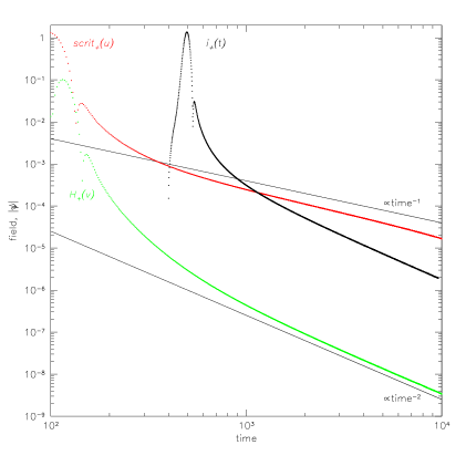
FIG. 2.: Time evolution of the scalar field from the Gaussian initial data. $i_{+}$ approximated by $\tilde{\psi}(y=400,t)$ represents future timelike inifinity while $scrit_{+}$ ($\tilde{\psi}(v=4\times 10^{4},u)$) and $H_{+}$ ($\tilde{\psi}(u=2\times 10^{4},v)$) represent future null infinity and the future horizon, respectively. Numerically calculated slopes for these curves are $-2.04$ for $i_{+}$, $-1.13$ for $scrit_{+}$, and $-1.99$ for $H_{+}$. Thin, solid lines have slopes equal to power-law exponents expected from theoretical predictions.

In Fig. 3 we examine the dependence of power-law exponents on the $l$-number. We studied the behaviour of the field on future timelike infinity $i_{+}$ for $l=0,1,2$. As in the previous example the thin solid lines indicate the theoretically predicted values of power-law exponents from Eq. (19). Once again the late time the power-law tails of the field converge to those theoretically predicted.

FIG. 3.: Field evolution on future timelike infinity, $i_{+}$, for different values of the parameter $l=0,1,2$. Curves have slopes of $-2.04$, $-4.07$, and $-6.06$, respectively. Thin solid lines indicate power- law exponents predicted from analytical investigations.

In order to check the late time behaviour of the field depends on the charge $Q$ we performed the calculation for two values of $(Q/M)^{2}$ ratios $0.1$ and $0.9$. For the Gaussian initial data with $l=0$. The results are presented in Fig. 4. Once again the theoretical predictions are in agreement with the numerical simulation. Fig. 4 envisages the evidence for the existence of power-law tails on the outer horizon of dilaton black hole for generic perturbations being of a great importance for the mass inflation scenario. For the first time the existence of power-law tails on the outer horizon of RN black hole was revealed in [4] studing a scalar field perturbations and also confirmed for the case of a massless charged scalar fields on RN background [6, 8].

FIG. 4.: Field evolution on future timelike infinity for different values of $(Q/M)^{2}$. Power-law exponents of the late-time tails are $-2.07$ for $(Q/M)^{2}=0.1$ and $-1.98$ for $(Q/M)^{2}=0.9$.

IV Conclusions

In our work we studied the asymptotic late-time behaviour of a massless charged scalar field in the background of dilaton black hole being the spherical solution of the so-called low-energy string theory. We confined the existence of oscillatory inverse power-law tails in a collapsing spacetime along asymptotic regions of future timelike infinity, future null infinity and along the outer horizon of the considered black hole.

On a null grid $(u,v)$ we integrated numerically the linearized charged scalar field Eqs. and confirmed the existence of the power-law tails. One also treated the dependence on the $l$-number, they converged to the results theoretically predicted. The numerical results confirmed our analytical conjecture that a charged hair decayed slower than a neutral one. The same statement was also revealed in RN case [6, 8]. The oscillatory inverse power-law tails along the outer horizon of dilaton black hole suggests the occurence of mass inflation along the Cauchy horizon of a dynamically formed dilaton black hole. It will be interesting to study the fully nonlinear gravitational collapse using a different scheme based on double null coordinates [15] which allows one to begin with regular initial conditions and continue the evolution all the way inside black hole. We hope to return to this problem elsewhere. Another problem for investigations is the problem of late-time behaviour of self-interacting scalar fields in the spacetime of dilaton black hole and the higher order string corrections modifying the initial action. [16].

Acknowledgements:
RM was partially supported by the Long Term Astrophysics grant NASA-NAG-6337 and NSF grant No. AST-9529175. MR was supported in part by KBN grant 2 P03B 093 18.

REFERENCES

-
[1]
M.Heusler, Black Holes Uniqueness Theorems
(Cambridge University Press, Cambridge, England, 1996),
K.S.Thorne, Black Holes and Time Warps (W.W.Norton and Company, New York, 1994). - [2] E.Poisson and W.Israel, Phys. Rev. D 41, 1796 (1990).
- [3] R.H.Price, Phys. Rev. D 5, 2419 (1972).
- [4] C.Gundlach, R.H.Price and J.Pullin, Phys. Rev. D 49, 883 (1994).
- [5] J.Bicak, Gen. Rel. Grav. 3, 331 (1972).
- [6] S.Hod and T.Piran, Phys. Rev. D 58, 024017 (1998).
- [7] S.Hod and T.Piran, Phys. Rev. D 58, 024018 (1998).
- [8] S.Hod and T.Piran, Phys. Rev. D 58, 024019 (1998).
- [9] S.Hod and T.Piran, Phys. Rev. D 58, 044018 (1998).
- [10] L.M.Burko, Abstracts of plenary talks and contributed papers, 15th International Conference on General Relativity and Gravitation, Pune, 1997, p.143, unpublished.
- [11] H.Koyama and A.Tomimatsu, Phys. Rev. D 63, 064032 (2001).
- [12] H.Koyama and A.Tomimatsu, gr-qc 0103086 (2001).
- [13] S.W.Hawking and G.R.F.Ellis, The Large Scale Structure of Space-Time (Cambridge University Press, Cambridge, England, 1973).
-
[14]
D.Garfinkle, G.T.Horowitz, and A.Strominger, Phys. Rev. D 43, 3140 (1991),
C.F.E.Holzhey and F.Wilczek, Nucl. Phys. B 380, 447 (1992). -
[15]
P.R.Brady and J.D.Smith, Phys. Rev. Lett. 75, 1256 (1995),
S.Hod and T.Piran, Phys. Rev. Lett. 81, 1554 (1998). - [16] R.Moderski and M.Rogatko (work in preparation).