On Symplectic, Multisymplectic Structures-Preserving
in Simple Finite Element Method

Han-Ying GUO¹, Xiao-mei JI ^1,2 Yu-Qi LI¹ and Ke WU¹

Abstract

    By the simple finite element method, we study the symplectic, multisymplectic structures and relevant preserving properties in some semi-linear elliptic boundary value problem in one-dimensional and two-dimensional spaces respectively. We find that with uniform mesh, the numerical schemes derived from finite element method can keep a preserved symplectic structure in one-dimensional case and a preserved multisymplectic structure in two-dimentional case respectively. These results are in fact the intrinsic reason that the numerical experiments indicate that such finite element schemes are accurate in practice.

Keywords: symplectic structure, finite element method, numerical scheme

1 Introduction

    It is well-known that the advantage of the finite element method is to adapt the flexible and complicated unstructured grids, whose mathematical theory is more profound and complete [1], and the systems to deal with by the method are Lagrangian ones in general. On the other hand, the symplectic algorithm [2] and multisymplectic algorithm [3] are also very powerful and successful for the finite and infinite dimensional Hamiltonian systems respectively in comparison with other non-symplectic and/or non-multi symplectic schemes. Therefore, there is a very natural but important and intriguing problem. Namely, what is the relation between these two extremely important aspects in scientific computing. More concretely, whether there exist some preserved symplectic and/or multisymplectic structures in finite element schemes. As far as we know, it is still an open problem.

In this paper, we study and definitely answer this problem by exploring certain concrete samples. We consider the boundary value problem of semi-linear elliptic equation with ordinary finite element schemes. In this method, we use linear elements for the spatial discretization. With uniform mesh, we have found that there exist certain preserved symplectic structure in one-dimensional space and certain multisymplectic structure that is also preserved in the discretized sense of the finite element method in two-dimensional space.

In the structure-preserving point of view, these results in fact are intrinsic reason why the numerical experiments state that such finite element algorithms are accurate in practice.

In what follows, we first consider the symplectic and multisymplectic geometry for the semi-linear elliptic equation in one-dimensional and two-dimensional spaces for both continuous and difference discrete cases in section 2. By introducing the Euler-Lagrange (EL) 1-forms, i.e. the null EL 1-form is given as the equation producting by a certain relevant 1-form which is cohomologically equivalent to the coboundary EL 1-forms, and EL condition, i.e. the closed EL 1-forms as well as their difference discrete versions [4] [5], we show that the symplectic structure in one-dimensional case and the multisymplectic structure in two-dimensional case and their difference discrete versions are preserved in the relevant configuration spaces in general rather than in the solution spaces of the equations only. In section 3, we briefly introduce relevant issues by the finite element scheme in one-dimensional and two-dimensional spaces for the boundary problem of the semi-linear elliptic equation. In section 4, we study the discrete versions of the symplectic and multisymplectic structures in the one-dimensional and two-dimensional finite element method for the semi-linear elliptic equation given in the section 3. We find explicitly the discrete versions of the symplectic and multisymplectic structures and their preserving properties respectively. Finally, we end with some remarks.

2 Symplectic geometry for semi-linear elliptic equation in 1-D and 2-D spaces

    In this paper, we consider the boundary value problem of the semi-linear elliptic equation in one-dimensional and two-dimensional spaces:

$$\triangle u=f(u)\quad in\quad\Omega,\quad u|_{\partial{\Omega}}=0\quad on\quad\partial\Omega.$$ (1)

$\Omega$ is a bounded domain in ${I\!\!R}^{n}$, $n=1,2$ and $f(u)$ is nonlinear and sufficiently smooth enough.

The weak formulation of the boundary value problem of the equation is: to find $u:\Omega\rightarrow H^{1}_{0}(\Omega)$ such that

$$\int_{\Omega}\nabla u\cdot\nabla vdx=-\int_{\Omega}f\cdot vdx\hskip 14.22636pt\forall v\in H^{1}_{0}(\Omega).$$ (2)

Let

$$a(u,v)=\int_{\Omega}\nabla u\cdot\nabla vdx,\quad(f,v)=-\int_{\Omega}f\cdot vdx,$$

then (2) becomes,

$$a(u,v)=(f,v).$$ (3)

It is important to note that in the one-dimensional case the equation is in fact an ODE with Lagrangian on ${I\!\!R}^{1}$. In the two-dimensional case the equation is also the one with Lagrangian. Therefore, in the continuous cases, they should be symplectic structure-preserving and multisymplectic structure-preserving respectively [2] [3] [4]. In this section, we briefly recall these facts with the help of the relevant Euler-Lagrange (EL) cohomology[4]. For the details of the symplectic and multisymplectic structures in the Lagrangian formalism, it can be found in [7] [8] [4]. The discrete versions of this kind of symplectic and multisymplectic structures are also derived from discrete variational principle [6] [7] [8] [4].

2.1 Symplectic structure in 1-D space case

    In one-dimensional space, the semi-linear equation becomes

$$u_{xx}=f(u)\quad in\quad\Omega,\quad u|_{\partial{\Omega}}=0\quad on\quad\partial\Omega.$$ (4)

where $u_{x}$ denotes the derivative of $u$ with respect to $x$, which is the coordinate of $\Omega$ and $\Omega$ a segment bounded domain in ${I\!\!R}^{1}$.

Let us first release both $u$ and $u_{x}$ from the solution space of the equation to the function space on $\Omega$. In order to do so, we introduce the EL 1-forms in the function space [4]

$$E(u,u_{x}):=\{u_{xx}-f(u)\}du,$$ (5)

and the EL condition [4], i.e. the EL 1-form is closed

$$dE(u,u_{x})=0,$$ (6)

leads to the symplectic structure and its preserving law.

It is easy to see that the null EL 1-form is equivalent to the equation. And it is a special case of the coboundary EL 1-forms given by,

$$E(u,u_{x})=d\alpha(u,u_{x}),$$ (7)

where $\alpha(u,u_{x})$ is an arbitrary function of $(u,u_{x})$ in the function space, automatically satisfying the EL condition. It is cohomologically trivial and equivalent to the null 1-form. Therefore, $u$ and $u_{x}$ in the EL 1-forms $E(u,u_{x})$ are Not in the solution space of the equation in general.

We may now introduce a new variable

$$v=u_{x}$$

in the function space and the EL condition becomes

$$v=u_{x},\quad d\{\{v_{x}-f(u)\}du\}=0,$$ (8)

Now it is easy to prove that the EL condition in the function space leads directly to the following equation:

$$\frac{d}{dx}\{dv\wedge du\}=0.$$ (9)

This means that there exists an intrinsic symplectic 2-form

$$\omega=dv\wedge du,$$ (10)

and it is divergence free in the sense

$$\frac{d}{dx}\omega=0.$$ (11)

In other words, the one-dimensional equation under consideration is symplectic structure-preserving.

We may also eliminate the variable $v$ to get symplectic 2-form in the Lagrangian formalism for the one-dimensional semi-linear elliptic equation as follows:

$$\omega=du_{x}\wedge du,$$ (12)

which is also preserved in the sense of divergence free

$$\frac{d}{dx}\omega=0.$$ (13)

In order to discretize the equation, we may take the difference with equal spatial step $h$ for the independent variable $x$,

$$x^{(n+1)}=x^{(n)}+h,\quad n=0,\cdots,N.$$

Then we may get the numerical integrator for the equation. For example,

$$u^{(n+1)}-u^{(n)}=hv^{(n)},\quad v^{(n+1)}-v^{(n)}=hf(u^{(n+1)}).$$ (14)

It is symplectic structure-preserving scheme in the following sense

$$dv^{(n+1)}\wedge du^{(n+1)}=dv^{(n)}\wedge du^{(n)}.$$ (15)

We will explain this issue later.

For the discrete case in difference, the discrete Euler-Lagrange (DEL) equation or the numerical scheme can be written as

$$u^{(n+2)}-2u^{(n+1)}+u^{(n)}=h^{2}f(u^{(n+1)}).$$ (16)

It can be proved that it is discretely symplectic structure-preserving [4]. The major points are as follows.

Introducing the DEL 1-form

$$E_{D}^{(n+1)}:=\{u^{(n+2)}-2u^{(n+1)}+u^{(n)}-h^{2}f(u^{(n+1)})\}du^{(n+1)},$$ (17)

the null DEL 1-form gives the DEL equation and also is a special case of the coboundary DEL 1-forms

$$E_{D}^{(n+1)}=d\alpha_{D}^{(n+1)}(u^{(n+1)}),$$ (18)

where $\alpha_{D}^{(n+1)}(u^{(n+1)})$ is an arbitrary function of $u^{(n+1)}$. Let us consider the DEL condition, i.e. the closed DEL 1-forms

$$dE_{D}^{(n+1)}=0.$$ (19)

It is straightforward to prove that from the DEL condition, it follows the symplectic preserving property:

$$du_{x}^{(n+1)}\wedge du^{(n+1)}=du_{x}^{(n)}\wedge du^{(n)},$$ (20)

where $u_{x}^{(n)}$ denotes the difference of $u$ at $x^{(n)}$ and the discrete symplectic 2-form is given by[6] [7] [8] [4] [5],

$$\omega_{D}^{(n)}=du_{x}^{(n)}\wedge du^{(n)}.$$ (21)

2.2 Multisymplectic structure in 2-D space case

    In the two-dimensional case, the semi-linear equation becomes

$$u_{x_{1}x_{1}}+u_{x_{2}x_{2}}=f(u)\quad in\quad\Omega,\quad u|_{\partial{\Omega}}=0\quad on\quad\partial\Omega.$$ (22)

where $u_{x_{i}}$, $i=1,2$, denote the partial derivative of $u$ w.r.t. $x_{i}$, $x_{i}$ the coordinates of $\Omega$ and $\Omega$ a bounded domain in ${I\!\!R}^{2}$.

Similar to the case of one-dimensional space, we can also introduce the EL 1-form,

$$E(u,u_{x_{i}}):=\{u_{x_{1}x_{1}}+u_{x_{2}x_{2}}-f(u)\}du,$$ (23)

such that the null EL 1-form is equivalent to the equation. And the coboundary EL 1-forms, i.e.

$$E(u,u_{x_{i}})=d\alpha(u,u_{x_{i}}),$$

where $\alpha(u,u_{x_{i}})$ is an arbitrary function of $(u,u_{x_{i}})$, are cohomologically equivalent to the null EL 1-form and they are cohomologically trivial.

Let us consider the following EL condition, i.e. the closed EL 1-forms

$$dE(u,u_{x_{i}})=0.$$ (24)

It is easy to see that $u(x_{i})$’s in the cohomological class are not the solution of the equation in general.

We may introduce two new variables in the function space on $\Omega$

$$v=u_{x_{1}},\quad w=u_{x_{2}}.$$ (25)

Then the EL condition becomes

$$v=u_{x_{1}},\quad w=u_{x_{2}},\quad d\{\{\frac{\partial}{\partial x_{1}}v+\frac{\partial}{\partial x_{2}}w-f(u)\}du\}=0,$$ (26)

where $(u,v,w)$ are in the function space on $\Omega$ rather than in the solution space of the equation only. By making use of the nilpotency of $d$, i.e. $d^{2}=0,$ it follows from the EL condition that

$$\frac{\partial}{\partial x_{1}}\{dv\wedge du\}+\frac{\partial}{\partial x_{2}}\{dw\wedge du\}=0.$$ (27)

This means that there are two intrinsic symplectic 2-forms

$$\omega=dv\wedge du,\quad\quad\tau=dw\wedge du.$$ (28)

and they are preserved in the sense of divergence free

$$\frac{\partial}{\partial x_{1}}\omega+\frac{\partial}{\partial x_{2}}\tau=0.$$ (29)

Therefore, the two-dimensional equation under consideration has what is called multisymplectic structure-preserving law that holds not only in the solution space but also in the function space under condition (24) as well.

For the difference discretized version, one of the discrete versions for the DEL equations or the numerical schemes can be given by,

$$\frac{u_{(i+1,j)}-2u_{(i,j)}+u_{(i-1,j)}}{{\Delta x_{1}}^{2}}+\frac{u_{(i,j+1)}-2u_{(i,j)}+u_{(i,j-1)}}{{\Delta x_{2}}^{2}}=f(u_{(i,j)}),$$ (30)

where $\Delta x_{i}$, $i=1,2$ are difference step-length in $x_{i}$.

We can also release $u_{(i,j)}$ ’s from the solution space to the function space by introducing the DEL 1-forms

$$E_{D}:=\{\frac{u_{(i+1,j)}-2u_{(i,j)}+u_{(i-1,j)}}{{\Delta x_{1}}^{2}}+\frac{u_{(i,j+1)}-2u_{(i,j)}+u_{(i,j-1)}}{{\Delta x_{2}}^{2}}-f(u_{(i,j)})\}du_{(i,j)},$$ (31)

and the null DEL 1-form is equivalent to the DEL equation as in the continuous case [4]. For the coboundary DEL 1-forms which are cohomologically trivial and equivalent to the null DEL 1-form. Then for the DEL 1-forms, specially for the closed DEL 1-forms, i.e. they satisfy the DEL condition

$$dE_{D}=0,$$ (32)

the $u_{(i,j)}$’s are in the function space in general rather than in the solution space only. Then it is straightforward from the DEL condition to get the discrete divergence free equations, i.e. the discrete multisymplectic structure-preserving property as follows:

$$\frac{1}{{\Delta x_{1}}^{2}}D_{x_{1}}(du_{x_{1}(i,j)}\wedge du_{(i,j)})+\frac{1}{{\Delta x_{2}}^{2}}D_{x_{2}}(du_{x_{2}(i,j)}\wedge du_{(i,j)})=0,$$ (33)

where $u_{x_{i}}$ is the difference of $u$ along $x_{i}$. These differences can be expressed as

$$D_{x_{1}}=E_{x_{1}}-1,\quad D_{x_{2}}=E_{x_{1}}-1,$$

and

$$E_{x_{1}}u_{(i,j)}=u_{(i+1,j)},\quad E_{x_{2}}u_{(i,j)}=u_{(i,j+1)}.$$

3 Finite element method in 1-D and 2-D spaces

    In this section, we consider certain spacial discretization and derive the relevant finite element schemes for the equation (1) in one-dimensional and two-dimensional cases. The problem on existence and uniqueness of the (weak) solution of schemes derived from finite element method for the semi-linear elliptic boundary problem will be given in [11]. In the next section we will show that the derived schemes in one-dimensional and two-dimensional cases are discretely symplectic and multisymplectic structure-preserving respectively.

3.1 Finite element scheme in one-dimensional space case

    Let $\Omega$ be a segment, $x_{i}$ the node, $\varphi_{i}$ shape function such that $\varphi_{i}(x_{j})=\delta_{ij}$, ${\cal T}$ the set of elements neighboring for given $x_{i}$, $\Omega_{i}=\cup_{T\in{\cal T}}T$, and $I_{T}$ the index set of the nodes of $T$ besides $x_{i}$. As usual, $u_{i}=u(x_{i})$. Let

$$u_{h}=\sum_{i=1}^{N_{1}}u_{i}\varphi_{i},\quad v_{h}=\sum_{i=1}^{N_{1}}v_{i}\varphi_{i},$$

so

$$a(u_{h},v_{h})=a(\sum_{j=1}^{N_{1}}u_{j}\varphi_{j},\sum_{i=1}^{N_{1}}v_{i}\varphi_{i}),\quad(f,v_{h})=(f,\sum_{i=1}^{N_{1}}v_{i}\varphi_{i}).$$

By the definition of weak solution, $a(u_{h},v_{h})=(f,v_{h})$, $\forall v_{i}$, we obtain

$$a(\sum_{j=1}^{N_{1}}u_{j}\varphi_{j},\varphi_{i})=(f,\varphi_{i}),\quad i=1,2,...,N_{1}.$$

we can get the finite element scheme as follows

$$\frac{u_{i+1}-2u_{i}+u_{i-1}}{h}=-(f(\sum_{i-1}^{i+1}u_{k}\varphi_{k}),\varphi_{i}).$$ (34)

3.2 Finite element scheme in two-dimensional space case

    Let $\Omega$ be a bounded polygonal domain in ${I\!\!R}^{2}$, $x_{i,j}$ the nodes, and $\varphi_{i,j}$ shape function such that $\varphi_{i,j}(x_{k,l})=\delta_{i,k}\delta_{j,l}$. For given $x_{i,j}$, let ${\cal T}$ be the set of elements neighboring $x_{i,j}$, $\Omega_{i,j}=\cup_{T\in{\cal T}}T$, and $u(x_{i,j})=u_{i,j}$. Similar to one-dimensional case, we can get the finite element scheme:

$$a(\sum_{i,j=1}^{N_{1}}u_{i,j}\varphi_{i,j},\varphi_{i,j})=-(f,\varphi_{i,j}),\quad i,j=1,2,...,N_{1}.$$ (35)

For $n=2$ we assume $\Omega$ is a square domain, and the mesh is uniform, that is, the plane ${I\!\!R}^{2}$ is divided into squares $\{x;i_{1}h\leq x_{1}\leq(i_{1}+1)h,i_{2}h\leq x_{2}\leq(i_{2}+1)h\},i_{1},i_{2}=0,\pm 1,\pm 2,\cdots$, and each square is further divided into two triangles by a straight line $x_{2}=x_{1}+ih$, $i$ integer. Take the node $x_{i,j}$ and $\Omega_{i,j}$ shown as figure 1. The elements are divided into two categories: the first category is shown as figure 2 and the second is shown as figure 3. For each element in the first category, the element stiff matrix is:

$$(a_{ij})=\begin{pmatrix}&\frac{1}{2}&-\frac{1}{2}&0\\ &-\frac{1}{2}&1&-\frac{1}{2}\\ &0&-\frac{1}{2}&\frac{1}{2}\\ \end{pmatrix},$$

For each element in the second category, the element stiff matrix is

$$(a_{ij})=\begin{pmatrix}&\frac{1}{2}&0&-\frac{1}{2}\\ &0&\frac{1}{2}&-\frac{1}{2}\\ &-\frac{1}{2}&-\frac{1}{2}&1\\ \end{pmatrix}.$$

We can get the finite element scheme as follows

$$u_{i,j+1}+u_{i+1,j}+u_{i,j-1}+u_{i-1,j}-4u_{i,j}$$

$$=\int_{\Omega_{i,j}}f(\sum u_{k,l}\varphi_{k,l})\varphi_{i,j}dx.$$ (36)

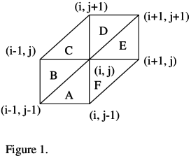
Figure 1:

Figure 2:

Figure 3:

4 The symplectic and multisymplectic structures in the 1-D and 2-D finite element methods

4.1 The symplectic structure in 1-D space

    In the case of 1-dimensional space, the equation (1) becomes an ODE as follows

$$u_{xx}=f(u)\quad u|_{\partial{\Omega}}=0,$$ (37)

where $x\in\Omega$, $\Omega$ is a segment of ${I\!\!R}^{1}$ with regular discretization of equal spatial step $h$.

From the finite element method, we get the scheme in last section

$$\frac{u_{i+1}-2u_{i}+u_{i-1}}{h}=\int_{i-1}^{i+1}f(\sum_{i-1}^{i+1}u_{k}\varphi_{k})\varphi_{i}dx.$$ (38)

The right side can be rewritten as

$$I_{i}:=\int_{i-1}^{i}f(u_{i-1}\varphi_{i-1}+u_{i}\varphi_{i})\varphi_{i}dx+\int_{i}^{i+1}f(u_{i}\varphi_{i}+u_{i+1}\varphi_{i+1})\varphi_{i}dx.$$ (39)

It should be noted as before that the variables $u_{i}$’s in the scheme can be released from the solution space to the function space by means of relevant DEL cohomologically equivalent relation. Therefore, as long as working with the DEL cohomology class associated with the DEL equation, the $u_{k}$’s can be regarded as in the function space in general rather than in the solution space only.

Introducing the DEL 1-forms

$$E_{Di}:=\{{u_{i+1}-2u_{i}+u_{i-1}}-hI_{i}\}du_{i},$$ (40)

such that the null DEL 1-form gives rise to the equation in the finite element method. Considering the coboundary DEL 1-form

$$E_{Di}=d\alpha_{Di},$$ (41)

where $\alpha_{Di}$ an arbitrary function on the function space, the null DEL 1-form is a special case of them. The DEL condition reads

$$dE_{Di}=0.$$ (42)

Namely, the DEL 1-forms are closed. Then it is easy to see that the variables $u_{i}$’s in the DEL 1-forms are in the function space in general and it is straightforward to see that from the DEL condition it follows

$$du_{i+1}\wedge du_{i}+du_{i-1}\wedge du_{i}$$ (43)

$$= h(\int_{i-1}^{i}f^{\prime}(u_{i-1}\varphi_{i-1}+u_{i}\varphi_{i})\varphi_{i-1}\varphi_{i}dx)du_{i-1}\wedge du_{i}$$

$$\quad+ h(\int_{i}^{i+1}f^{\prime}(u_{i}\varphi_{i}+u_{i+1}\varphi_{i+1})\varphi_{i+1}\varphi_{i}dx)du_{i+1}\wedge du_{i},$$

i.e.,

$$(1-h\int_{i}^{i+1}f^{\prime}(u_{i}\varphi_{i}+u_{i+1}\varphi_{i+1})\varphi_{i+1}\varphi_{i}dx)du_{i+1}\wedge du_{i}$$ (44)

$$= (1-h\int_{i-1}^{i}f^{\prime}(u_{i-1}\varphi_{i-1}+u_{i}\varphi_{i})\varphi_{i-1}\varphi_{i}dx)du_{i}\wedge du_{i-1}.$$

Let us define a 2-form as

$$\omega^{(i+1)}=(1-h\int_{i}^{i+1}f^{\prime}(u_{i}\varphi_{i}+u_{i+1}\varphi_{i+1})\varphi_{i+1}\varphi_{i}dx)du_{i+1}\wedge du_{i}.$$ (45)

It can be checked that this 2-form is closed with respect to $d$ on the function space and its coefficients are non-degenerate, so that it is a symplectic structure for the scheme derived from finite element method in the case of one-dimensional space and it is preserved in the sense

$$\omega^{(i+1)}=\omega^{(i)}.$$ (46)

4.2 Multisymplectic structure in 2-D space case

    Now we discuss the following semi-linear equation

$$u_{x_{1}x_{1}}+u_{x_{2}x_{2}}=f(u),$$ (47)

where $x_{1},x_{2}$ are coordinates in ${I\!\!R}^{2}$. We first discrete ${I\!\!R}^{2}$ with regular lattice ${I\!\!L}^{2}={I\!\!L}^{1}\otimes{I\!\!L}^{1}$, and ${I\!\!L}^{1}$ is of equal spatial step $h$.

The discrete scheme for this equation form finite element method is given by (36) as follows

$$u_{i,j+1}+u_{i+1,j}+u_{i,j-1}+u_{i-1,j}-4u_{i,j}$$

$$=\int_{\Omega_{i,j}}f(\sum u_{k,l}\varphi_{k,l})\varphi_{i,j}dx,$$

where the shape function $\varphi_{i,j}$ is linear continuous function defined as

$$\varphi_{i,j}(x_{k,l})=\delta_{i.k}\delta_{j,l}.$$

The right side of (36) can be denoted by

$$I_{\Omega_{i,j}} := \int_{\Omega_{i,j}}f(\sum u_{k,l}\varphi_{k,l})\varphi_{i,j}dx$$ (48)

$$= (\int_{A}+\int_{B}+\int_{C}+\int_{D}+\int_{E}+\int_{F})f(\sum u_{k,l}\varphi_{k,l})\varphi_{i,j}dx,$$

where

$$I_{\Omega_{i,j}A} := \int_{A}f(\sum u_{k,l}\varphi_{k,l})\varphi_{i,j}dx$$

$$= \int_{A}f(u_{i-1,j-1}\varphi_{i-1,j-1}+u_{i,j-1}\varphi_{i,j-1}+u_{i,j}\varphi_{i,j})\varphi_{i,j}dx.$$

$$I_{\Omega_{i,j}B} := \int_{B}f(\sum u_{k,l}\varphi_{k,l})\varphi_{i,j}dx$$

$$= \int_{B}f(u_{i-1,j-1}\varphi_{i-1,j-1}+u_{i-1,j}\varphi_{i-1,j}+u_{i,j}\varphi_{i,j})\varphi_{i,j}dx$$

$$I_{\Omega_{i,j}C} := \int_{C}f(\sum u_{k,l}\varphi_{k,l})\varphi_{i,j}dx$$

$$= \int_{C}f(u_{i-1,j}\varphi_{i-1,j}+u_{i,j}\varphi_{i,j}+u_{i,j+1}\varphi_{i,j+1})\varphi_{i,j}dx$$

$$I_{\Omega_{i,j}D} := \int_{D}f(\sum u_{k,l}\varphi_{k,l})\varphi_{i,j}dx$$

$$= \int_{D}f(u_{i+1,j+1}\varphi_{i+1,j+1}+u_{i,j}\varphi_{i,j}+u_{i,j+1}\varphi_{i,j+1})\varphi_{i,j}dx$$

$$I_{\Omega_{i,j}E} := \int_{E}f(\sum u_{k,l}\varphi_{k,l})\varphi_{i,j}dx$$

$$= \int_{E}f(u_{i+1,j+1}\varphi_{i+1,j+1}+u_{i,j}\varphi_{i,j}+u_{i+1,j}\varphi_{i+1,j})\varphi_{i,j}dx$$

$$I_{\Omega_{i,j}F} := \int_{F}f(\sum u_{k,l}\varphi_{k,l})\varphi_{i,j}dx$$

$$= \int_{F}f(u_{i+1,j}\varphi_{i+1,j}+u_{i,j}\varphi_{i,j}+u_{i,j-1}\varphi_{i,j-1})\varphi_{i,j}dx.$$

where the sub-index $A,B,C,D,E,F$ indicate the all elements neighboring $x_{i,j}$ in Figure 1.

Similar to the one-dimensional case, introducing the DEL 1-forms

$$E_{D\Omega_{i,j}}:=\{u_{i,j+1}+u_{i+1,j}+u_{i,j-1}+u_{i-1,j}-4u_{i,j}-I_{\Omega_{i,j}}\}du_{i,j},$$ (49)

such that the null DEL 1-form gives rise to the equation (36) in the finite element method. The coboundary DEL 1-forms are given by

$$E_{D\Omega_{i,j}}=d\alpha_{D\Omega_{i,j}},$$ (50)

where $\alpha_{D\Omega_{i,j}}$ an arbitrary function in the function space on $\Omega_{i,j}$. And the null DEL 1-form is a special case of them.

The DEL condition now reads

$$dE_{D\Omega_{i,j}}=0.$$ (51)

Although the null DEL 1-form gives rise to the equation and satisfies automatically the DEL condition, but in general

the $u_{j,k}$’s are still unknown functions rather than the ones in the solution space of the equation.

It is also straightforward to see that

in the function space it follows from the DEL condition that

$$du_{i,j+1}\wedge du_{i,j}+du_{i+1,j}\wedge du_{i,j}+du_{i,j-1}\wedge du_{i,j}+du_{i-1,j}\wedge du_{i,j}$$ (52)

$$= \int_{D}f^{\prime}(u_{i+1,j+1}\varphi_{i+1,j+1}+u_{i,j}\varphi_{i,j}+u_{i,j+1}\varphi_{i,j+1})\varphi_{i+1,j+1}\varphi_{i,j}dx\cdot du_{i+1,j+1}\wedge du_{i,j}$$

$$+ \int_{D}f^{\prime}(u_{i+1,j+1}\varphi_{i+1,j+1}+u_{i,j}\varphi_{i,j}+u_{i,j+1}\varphi_{i,j+1})\varphi_{i,j+1}\varphi_{i,j}dx\cdot du_{i,j+1}\wedge du_{i,j}$$

$$+ \int_{E}f^{\prime}(u_{i+1,j+1}\varphi_{i+1,j+1}+u_{i,j}\varphi_{i,j}+u_{i+1,j}\varphi_{i+1,j})\varphi_{i+1,j+1}\varphi_{i,j}dx\cdot du_{i+1,j+1}\wedge du_{i,j}$$

$$+ \int_{E}f^{\prime}(u_{i+1,j+1}\varphi_{i+1,j+1}+u_{i,j}\varphi_{i,j}+u_{i+1,j}\varphi_{i+1,j})\varphi_{i+1,j}\varphi_{i,j}dx\cdot du_{i+1,j}\wedge du_{i,j}$$

$$+ \int_{F}f^{\prime}(u_{i+1,j}\varphi_{i+1,j}+u_{i,j}\varphi_{i,j}+u_{i,j-1}\varphi_{i,j-1})\varphi_{i+1,j}\varphi_{i,j}dx\cdot du_{i+1,j}\wedge du_{i,j}$$

$$+ \int_{F}f^{\prime}(u_{i+1,j}\varphi_{i+1,j}+u_{i,j}\varphi_{i,j}+u_{i,j-1}\varphi_{i,j-1})\varphi_{i,j-1}\varphi_{i,j}dx\cdot du_{i,j-1}\wedge du_{i,j}$$

$$+ \int_{A}f^{\prime}(u_{i-1,j-1}\varphi_{i-1,j-1}+u_{i,j-1}\varphi_{i,j-1}+u_{i,j}\varphi_{i,j})\varphi_{i,j-1}\varphi_{i,j}dx\cdot du_{i,j-1}\wedge du_{i,j}$$

$$+ \int_{A}f^{\prime}(u_{i-1,j-1}\varphi_{i-1,j-1}+u_{i,j-1}\varphi_{i,j-1}+u_{i,j}\varphi_{i,j})\varphi_{i-1,j-1}\varphi_{i,j}dx\cdot du_{i-1,j-1}\wedge du_{i,j}$$

$$+ \int_{B}f^{\prime}(u_{i-1,j-1}\varphi_{i-1,j-1}+u_{i-1,j}\varphi_{i-1,j}+u_{i,j}\varphi_{i,j})\varphi_{i-1,j-1}\varphi_{i,j}dx\cdot du_{i-1,j-1}\wedge du_{i,j}$$

$$+ \int_{B}f^{\prime}(u_{i-1,j-1}\varphi_{i-1,j-1}+u_{i-1,j}\varphi_{i-1,j}+u_{i,j}\varphi_{i,j})\varphi_{i-1,j}\varphi_{i,j}dx\cdot du_{i-1,j}\wedge du_{i,j}$$

$$+ \int_{C}f^{\prime}(u_{i-1,j}\varphi_{i-1,j}+u_{i,j}\varphi_{i,j}+u_{i,j+1}\varphi_{i,j+1})\varphi_{i-1,j}\varphi_{i,j}dx\cdot du_{i-1,j}\wedge du_{i,j}$$

$$+ \int_{C}f^{\prime}(u_{i-1,j}\varphi_{i-1,j}+u_{i,j}\varphi_{i,j}+u_{i,j+1}\varphi_{i,j+1})\varphi_{i,j+1}\varphi_{i,j}dx\cdot du_{i,j+1}\wedge du_{i,j}.$$

Note that the right side is equal to the following terms that can be denoted as $S_{A\{i,j\}},\cdots,S_{F\{i,j\}}$.

$$S_{A\{i,j\}} = (\int_{D}f^{\prime}(u_{i+1,j+1}\varphi_{i+1,j+1}+u_{i,j}\varphi_{i,j}+u_{i,j+1}\varphi_{i,j+1})\varphi_{i+1,j+1}\varphi_{i,j}dx+$$

$$\int_{E}f^{\prime}(u_{i+1,j+1}\varphi_{i+1,j+1}+u_{i,j}\varphi_{i,j}+u_{i+1,j}\varphi_{i+1,j})\varphi_{i+1,j+1}\varphi_{i,j}dx)\cdot du_{i+1,j+1}\wedge du_{i,j},$$

$$S_{B\{i,j\}} = (\int_{D}f^{\prime}(u_{i+1,j+1}\varphi_{i+1,j+1}+u_{i,j}\varphi_{i,j}+u_{i,j+1}\varphi_{i,j+1})\varphi_{i,j+1}\varphi_{i,j}dx+$$

$$\int_{C}f^{\prime}(u_{i-1,j}\varphi_{i-1,j}+u_{i,j}\varphi_{i,j}+u_{i,j+1}\varphi_{i,j+1})\varphi_{i,j+1}\varphi_{i,j}dx)\cdot du_{i,j+1}\wedge du_{i,j},$$

$$S_{C\{i,j\}} = (\int_{E}f^{\prime}(u_{i+1,j+1}\varphi_{i+1,j+1}+u_{i,j}\varphi_{i,j}+u_{i+1,j}\varphi_{i+1,j})\varphi_{i+1,j}\varphi_{i,j}dx+$$

$$\int_{F}f^{\prime}(u_{i+1,j}\varphi_{i+1,j}+u_{i,j}\varphi_{i,j}+u_{i,j-1}\varphi_{i,j-1})\varphi_{i+1,j}\varphi_{i,j}dx)\cdot du_{i+1,j}\wedge du_{i,j},$$

$$S_{D\{i,j\}} = (\int_{F}f^{\prime}(u_{i+1,j}\varphi_{i+1,j}+u_{i,j}\varphi_{i,j}+u_{i,j-1}\varphi_{i,j-1})\varphi_{i,j-1}\varphi_{i,j}dx+$$

$$\int_{A}f^{\prime}(u_{i-1,j-1}\varphi_{i-1,j-1}+u_{i,j-1}\varphi_{i,j-1}+u_{i,j}\varphi_{i,j})\varphi_{i,j-1}\varphi_{i,j}dx)\cdot du_{i,j-1}\wedge du_{i,j},$$

$$S_{E\{i,j\}} = (\int_{A}f^{\prime}(u_{i-1,j-1}\varphi_{i-1,j-1}+u_{i,j-1}\varphi_{i,j-1}+u_{i,j}\varphi_{i,j})\varphi_{i-1,j-1}\varphi_{i,j}dx+$$

$$\int_{B}f^{\prime}(u_{i-1,j-1}\varphi_{i-1,j-1}+u_{i-1,j}\varphi_{i-1,j}+u_{i,j}\varphi_{i,j})\varphi_{i-1,j-1}\varphi_{i,j}dx)\cdot du_{i-1,j-1}\wedge du_{i,j},$$

$$S_{F\{i,j\}} = (\int_{B}f^{\prime}(u_{i-1,j-1}\varphi_{i-1,j-1}+u_{i-1,j}\varphi_{i-1,j}+u_{i,j}\varphi_{i,j})\varphi_{i-1,j}\varphi_{i,j}dx+$$

$$\int_{C}f^{\prime}(u_{i-1,j}\varphi_{i-1,j}+u_{i,j}\varphi_{i,j}+u_{i,j+1}\varphi_{i,j+1})\varphi_{i-1,j}\varphi_{i,j}dx)\cdot du_{i-1,j}\wedge du_{i,j}.$$

Note that all $S_{k\{i,j\}},k=A,\cdots,F$ are order of $h^{2}$.

Let us introduce two shift operators as

$$E_{1}f(u_{i,j})=f(u_{i+1,j}),$$

$$E_{2}f(u_{i,j})=f(u_{i,j+1}).$$

Then the following relations can be found

$$S_{A\{i,j\}} = -E_{1}E_{2}S_{E\{i,j\}},$$

$$S_{B\{i,j\}} = -E_{2}S_{D\{i,j\}},$$

$$S_{C\{i,j\}} = -E_{1}S_{F\{i,j\}},$$

$$du_{i,j+1}\wedge du_{i,j} = -E_{2}(du_{i,j-1}\wedge du_{i,j}),$$

$$du_{i+1,j}\wedge du_{i,j} = -E_{1}(du_{i-1,j}\wedge du_{i,j}).$$

It is easy to check that (52) becomes

$$(1-E_{2})(du_{i,j-1}\wedge du_{i,j})+(1-E_{1})(du_{i-1,j}\wedge du_{i,j})$$ (53)

$$= \{(1-E_{2}E_{1})S_{E\{i,j\}}+(1-E_{2})S_{B\{i,j\}}+(1-E_{1})S_{F\{i,j\}}\}.$$

Let us define

$$\omega_{D{i,j}}=du_{i-1,j}\wedge du_{i,j}-E_{2}S_{E\{i,j\}}-S_{F\{i,j\}},$$ (54)

$$\tau_{D{i,j}}=du_{i,j-1}\wedge du_{i,j}-S_{B\{i,j\}}-S_{E\{i,j\}}.$$ (55)

It is straightforward to show that $\omega_{D}$ and $\tau_{D}$ are two symplectic 2-forms. Namely, they are closed with respect to $d$ on the function space and non-degenerate. Then the equation (53) is in fact a discrete version of the multisymplectic conservation law as follows

$$D_{1}\omega_{D{i,j}}+D_{2}\tau_{D{i,j}}=0.$$ (56)

Here $D_{1}$ and $D_{2}$ are differences given by

$$D_{1}=E_{1}-1,\quad D_{2}=E_{2}-1,\quad$$ (57)

and they satisfy the relation

$$E_{2}E_{1}-1=D_{1}E_{2}+D_{2}.$$

5 Remarks

    In this paper we have explored the relations between symplectic and multisymplectic algorithms and the simple finite element method for the boundary value problem of the semi-linear elliptic equation in one-dimensional and two-dimensional spaces. Although what we have found are certain simple boundary value problem of the semi-linear elliptic equation in lower dimensions and also quite simple triangulization in the finite element method, the results still indicate that there should be very deep connections between the symplectic and/or multisymplectis algorithms and the finite element method. The discrete variational principle should be one of the key links between these two topics.

We have constructed the discrete symplectic 2-form in one-dimensional case and two discrete symplectic 2-forms in two-dimensional case and proved they are preserved in the sense of discretely divergence free. It is important to see that these results should be able to generalize to higher dimensional cases and more complicated boundary value problem. The most important point in our approach is that we work with the discrete Euler-Lagrange conditions rather than the discrete equations in the simple finite element method. Although they are cohomologically relevant, the discrete symplectic and discrete multisymplectic structures and their preserving properties hold not only in the solution space but also in the function space in general.

On the other hand, it should be mentioned that in this paper we have not employed the noncommutative differential calculus (NCDC). But, in principle some NCDC should be introduced in order to establish a more complete formulation for this issue [9] [10] [4]. The reason is very simple: since the space domain $\Omega$ (independent variables) is discretized in the finite element method, the ordinary differential calculus does not make precisely sense in order to construct the exterior forms in $\Omega$ and so forth. It should also be mentioned that the NCDC to be employed is also dependant on the triangulization version in the finite element method.

Finally, there are lots of relevant problems should to studied and some of them are under investigation. For instance, what about the symplectic or multisymplectic structure-preserving properties in the case for more complicated triangulation and boundary conditions etc. We will publish some results on these issues elsewhere.

References

- [1] P. G. Ciarlet, The Finite Element Method for Elliptic Problems, North-Holland, Amsterdam, 1978, and references therein. Selected Works of Feng Kang (I), Ed. by Z.C. Shi et. al. (1994), and references therein. C. Johnson, Numerical solution of partial differential equations by the finite element method. Cambridge University Press, 1994, and references therein. L.A. Ying, Notes of lectures about finite element method, (in Chieses) Peking University, (1986).
- [2] Selected Works of Feng Kang (II), Ed. by Z.C. Shi et. al. (1995), and references therein. J.M.Sanz-Serna and M.P.Calvo, Numerical Hamiltonian problem, (1994), Chapman and Hall, London, and references therein.
- [3] T.J. Bridges, multisymplectic structures and wave propagations, Math. Proc. Camb. Phil. Soc., 121 (1997)147-190. T.J. Bridges and S. Reich, multisymplectic integrators: numerical schemes for Hamiltonian PDEs that conserve symplecticity, preprint (1999). J.E. Marsden, G.W. Patrick and S.Shkoller, Multisymplectic geometry, variational integrators, and nonlinear PDEs, Commun. Math. Phys., 199 (1998) 351-395.
- [4] H.Y. Guo Y.Q. Li and K. Wu, On symplectic and multisymplectic structures and their discrete versions in Lagrangian formalism, ITP-preprint (March, 2001) hep-ph/0104064.
- [5] H.Y. Guo Y.Q. Li and K. Wu, A note on symplectic algorithms, ITP-preprint (March, 2001) physics/0104030.
- [6] A.P. Veselov, Integranble discrete-time system and difference operator, Funkts. Anal. Prilozhen., 22 (1988)1-13. J. Moser and A.P. Veselov, Discrete versions of some classical integrable systems and factorization of matrix polynomials, Commun. Math. Phys., 139 (1991)217-243.
- [7] J.M. Wendlandt and J.E. Marsden, Mechanical integrators derived from a discrete variation plinciple, Physica D 106 (1997)223-246.
- [8] Y.J. Sun and M.Z. Qin, Variational integrators and application for higher order differential equations, CCAST-WL workshop series: 118, 45-58.
- [9] H.Y. Guo, K.Wu, S.H. Wang, S.K. Wang and G.M.Wei, Noncommutative Differential Calculas Approach to Symplectic Algorithm on Regular Lattice, Comm. Theor. Phys., 34 (2000) 307-318.
- [10] H.Y.Guo, K.Wu and W.Zhang, Noncommutative Differential Calculus on Abelian Groups and Its Applications, Comm.Theor. Phys., 34 (2000) 245-250.
- [11] X.M. Ji, to appear.