A Geometrical Interpretation of Grassmannian Coordinates

Abstract

A geometrical interpretation of Grassmannian anticommuting coordinates is given. They are taken to represent an indefiniteness inherent in every spacetime point on the level of the spacetime foam. This indeterminacy is connected with the fact that in quantum gravity in some approximation we do not know the following information : are two points connected by a quantum wormhole or not ? It is shown that: (a) such indefiniteness can be represented by Grassmanian numbers, (b) a displacement of the wormhole mouth is connected with a change of the Grassmanian numbers (coordinates). In such an interpretation of supersymmetry the corresponding supersymmetrical fields must be described in an invariant manner on the background of the spacetime foam.

I Introduction

The idea of superspace enlarges the spacetime points labelled by the coordinates $x^{\mu}$ by adding two plus two anticommuting Grassmannian coordinates $\theta_{\alpha}$ and $\bar{\theta}_{\dot{\beta}}$ ($\alpha$ and $\dot{\beta}$ are the spinor indices). Thus the coordinates on superspace are $Z^{M}=(x^{\mu},\theta_{\alpha},\bar{\theta}_{\dot{\beta}})$ and for brevity we introduce $\theta=(\theta_{\alpha},\bar{\theta}_{\dot{\beta}})$. Ordinary anticommuting coordinates $\theta$ are abstract Grassmannian numbers. Nevertheless the following question should be asked : can the Grassmannian coordinates have some physical meaning ? In this paper I would like to show that a physical meaning can be given in terms of an indefiniteness inherent at every point of spacetime.

What kind of indefiniteness can be incorporated in spacetime ? We assume that such an indeterminacy can appear in quantum gravity on the level of the spacetime foam. The notion of the spacetime foam was introduced by Wheeler for describing the possible complex structure of spacetime on the Planck scale wheeler . It is postulated that the spacetime foam is a cloud of quantum wormholes with a typical linear size of the Planck length. Schematically in some rough approximation we can imagine the appearing/disappearing of quantum wormholes as pasting together two points with a subsequent break (see, Fig.1). In our approach we deliberately neglect the following information : whether two points $y^{\mu}$ and $x^{\mu}$ are connected by a quantum wormhole or not.

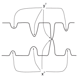
Figure 1: The wormhole in the spacetime foam as an identification of two points $y^{\mu}$ and $x^{\mu}$. We shall name such wormhole as in Ref. smolin : a minimalist wormhole. Such minimalist wormhole is an approximation of the real wormhole in which we neglect all linear sizes (longitudinal and cross section).

In such an approximation we have an indeterminacy for each spacetime point. We can say that in this approximation the spacetime foam in quantum gravity is described in some effective manner : quantum minimalist wormholes are approximated as an indefiniteness inherent in every spacetime point.

II Physical idea

Our assumption is that Grassmannian coordinate $\theta$ describes the indefiniteness (the loss of information) of our knowledge about two points $x^{\mu}$ and $y^{\mu}$ : we do not know if these points are connected by a quantum minimalist wormhole or not (see, Fig.2)

$$\theta=\left(\theta_{\alpha},\bar{\theta}_{\dot{\beta}}\right)=Id\left(x^{\alpha\dot{\beta}}\;\raisebox{6.45831pt}{$\underleftrightarrow{\scriptstyle{\;\;yes\;or\;no\;?\;\;}}$}\;y^{\alpha\dot{\beta}}\right)$$ (1)

where $Id(\ldots)$ is the designation for the identification procedure; $x_{\alpha\dot{\beta}}=\sigma_{\mu\alpha\dot{\beta}}x^{\mu}$; $\sigma^{\mu}_{\alpha\dot{\beta}}=\{\textbf{1},-\sigma^{i}\}$; $\sigma^{i}$ are the Pauli matrices; $\alpha,\dot{\beta}=1,2$ are the matrix indices; $\mu=0,1,2,3$ is the spacetime index; $i=1,2,3$ is the space index

$$x^{\alpha\dot{\beta}} = \varepsilon^{\alpha\gamma}\varepsilon^{\dot{\beta}\dot{\delta}}x_{\gamma\dot{\delta}},$$ (2)

$$\varepsilon^{\alpha\beta} = \varepsilon^{\dot{\alpha}\dot{\beta}}=\begin{pmatrix}0&1\\ -1&0\end{pmatrix},$$ (3)

$$\varepsilon_{\alpha\beta} = \varepsilon_{\dot{\alpha}\dot{\beta}}=\begin{pmatrix}0&-1\\ 1&0\end{pmatrix}.$$ (4)

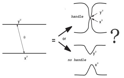
Figure 2: A geometrical interpretation of the Grassmannian coordinate $\theta$. The Grassmannian number $\theta$ describes the indefiniteness (the lack of knowledge) : are the points $y^{\mu}$ and $x^{\mu}$ identified or separated ?

Such an interpretation of $\theta$ is similar to the interpretation of spin : in certain situations we do not know the value of the $z-$ projection of spin $(\hbar/2$ or $-\hbar/2)$. In Pauli’s words spin is “a non-classical two-valuedness” or in the context of this paper it is an “indefiniteness” (“indeterminacy”). In modern terms “non-classical two-valuedness” is spin and it can be described only using spinors.

This comparison allows us to postulate that the above-mentioned indeterminacy connected with the spacetime foam (pasting together/cutting off of points) can be described using spinors. Let us introduce the scalar product for spinors $\psi$ and $\chi$ as (see, for example, Ref. bilal )

$$\psi\chi=\psi^{\alpha}\chi_{\alpha}=\varepsilon^{\alpha\beta}\psi_{\beta}\chi_{\alpha}.$$ (5)

For the scalar product should imply

$$\psi\chi=\chi\psi$$ (6)

but

$$\chi\psi=\varepsilon^{\alpha\beta}\chi_{\beta}\psi_{\alpha}$$ (7)

hence

$$\varepsilon^{\alpha\beta}\psi_{\beta}\chi_{\alpha}=-\varepsilon^{\alpha\beta}\chi_{\alpha}\psi_{\beta}$$ (8)

this means that

$$\psi_{\beta}\chi_{\alpha}=-\chi_{\alpha}\psi_{\beta},$$ (9)

i.e. the components of a spinor describing the above-mentioned indefiniteness are anticommuting Grassmannian numbers. These arguments allow us to say that the indefiniteness can be described using anticommuting Grassmannian coordinates.

III Spacetime foam and indefiniteness

III.1 Precedent results

In this subsection I would like to remind some definitions from Ref. smolin . Let us define an operator $\hat{A}(x,y)$ : it is an operator which identifies two points $x$ and $y$ or another words this operator creates a minimalist wormhole (see Fig. 1). It makes no sense to identify these points $(x,y)$ twice, therefore we have the following property

$$\left(\hat{A}(x,y)\right)^{2}=0.$$ (10)

Let us introduce Weyl fermion $\psi^{\alpha}(x)$ with the standard anticommuting relations

$$\left[\psi^{\alpha}(x),\psi^{\dagger}_{\beta}(y)\right]=\delta^{\alpha}_{\beta}\delta^{3}(x-y).$$ (11)

In the context of Ref. smolin we have the following relation between minimalist wormhole and Weyl fermion

$$\psi^{\alpha}(x)\psi^{\beta}(y)\Longleftrightarrow-\varepsilon^{\alpha\beta}\hat{A}(x,y).$$ (12)

Let us introduce an operator $\hat{B}(x\rightarrow x^{\prime})$ which moves a mouth of a wormhole from point $x$ to point $x^{\prime}$

$$\hat{B}(x\rightarrow x^{\prime})\hat{A}(y,x)=\hat{A}(y,x^{\prime}).$$ (13)

III.2 Mathematical definitions

In this subsection I would like to connect a modification of the operators $\hat{A}(x,y)$ and $B(x\rightarrow x^{\prime})$ introduced by Smolin with the Grassmanian coordinates.

Let we have an operator $\hat{A}^{AB}(x,y)$ describing a quantum state in which the space with two points $x$ and $y$ fluctuates between two possibilities : points $(x,y)$ either identified or not. Let the operator $\hat{A}^{AB}(x,y)$ like to the previous Smolin’s definition) has the following property

$$\hat{A}^{AB}(x,y)\hat{A}_{AB}(x,y)=0.$$ (14)

We should note that

• we do not here define the indices $(A,B)$;

• $\hat{A}_{AB}(x,y)=\epsilon_{AC}\epsilon_{BD}\hat{A}^{CD}(x,y)$ and the matrixes $\epsilon_{AB}$ we will define later.

The solution of Eq.(14) we search in the form

$$\hat{A}^{AB}(x,y)=\theta^{A}(x)\theta^{B}(y).$$ (15)

From Eq’s (14) and (15) we have

$$\theta^{A}(x)\theta^{B}(y)\theta_{A}(x)\theta_{B}(y)=0.$$ (16)

This equation has the following two simplest solution. The first is

$$A = \alpha,\;B=\beta,\;(\alpha,\beta=1,2),$$ (17)

$$\epsilon_{\alpha\beta} = \varepsilon_{\alpha\beta},$$ (18)

$$\hat{A}^{\alpha\beta}(x,y) = \varepsilon^{\alpha\beta}\hat{A}(x,y)=\theta^{\alpha}\theta^{\beta}.$$ (19)

It means that $\theta^{\alpha}$ is an undotted spinor of $(\frac{1}{2},0)$ representation of Sl(2,C) group.

$$\theta^{\alpha}(x) = \theta^{\alpha}(y)=\theta^{\alpha}=const,$$ (20)

$$\theta^{\alpha}\theta^{\beta} = -\theta^{\beta}\theta^{\alpha};\qquad\alpha\neq\beta,$$ (21)

$$\left(\theta^{\alpha}\right)^{2} = 0.$$ (22)

The second solution is the same but only with the replacement $\alpha\rightarrow\dot{\alpha}$ and $\beta\rightarrow\dot{\beta}$

$$A = \dot{\alpha},\;B=\dot{\beta},\;(\dot{\alpha},\dot{\beta}=1,2),$$ (23)

$$\epsilon_{\dot{\alpha}\dot{\beta}} = \varepsilon_{\dot{\alpha}\dot{\beta}},$$ (24)

$$\hat{A}^{\dot{\alpha}\dot{\beta}}(x,y) = \varepsilon^{\dot{\alpha}\dot{\beta}}\hat{A}(x,y)=\theta^{\dot{\alpha}}\theta^{\dot{\beta}},$$ (25)

$$\bar{\theta}^{\dot{\alpha}}(x) = \bar{\theta}^{\dot{\alpha}}(y)=\bar{\theta}^{\dot{\alpha}}=const,$$ (26)

$$\bar{\theta}^{\dot{\alpha}}\bar{\theta}^{\dot{\beta}} = -\bar{\theta}^{\dot{\beta}}\bar{\theta}^{\dot{\alpha}};\qquad\dot{\alpha}\neq\dot{\beta},$$ (27)

$$\left(\bar{\theta}^{\dot{\alpha}}\right)^{2} = 0.$$ (28)

In this case $\bar{\theta}^{\dot{\alpha}}$ is a dotted spinor of $(0,\frac{1}{2})$ representation. More concretely we have

$$\theta^{1}\theta^{2} = -\theta^{2}\theta^{1}\quad\text{or}\quad\bar{\theta}^{\dot{1}}\bar{\theta}^{\dot{2}}=-\bar{\theta}^{\dot{2}}\bar{\theta}^{\dot{1}},$$ (29)

$$\left(\theta^{1}\right)^{2} = \left(\theta^{2}\right)^{2}=\left(\bar{\theta}^{\dot{1}}\right)^{2}=\left(\bar{\theta}^{\dot{2}}\right)^{2}=0.$$ (30)

Such two-valuedness forces us to introduce both possibilities : $\theta=\{\theta^{\alpha},\bar{\theta}^{\dot{\alpha}}\}$.

Now we would like to introduce an infinitesimal operator $\delta\hat{B}(x^{\mu}\rightarrow{x^{\prime}}^{\mu})$ (like to Smolin) of a displacement of the wormhole mouth

$$\delta\hat{B}(x^{\mu} \rightarrow {x^{\prime}}^{\mu})\hat{A}^{\gamma\delta}(y^{\mu},x^{\mu})=\hat{A}^{\gamma\delta}(y^{\mu},{x^{\prime}}^{\mu}),$$ (31)

$$\hat{A}^{\gamma\delta}(y^{\mu},x^{\mu}) = \theta^{\gamma}\theta^{\delta},$$ (32)

$$\hat{A}^{\gamma\delta}(y^{\mu},{x^{\prime}}^{\mu}) = {\theta^{\prime}}^{\gamma}{\theta^{\prime}}^{\delta}=\left(\theta^{\gamma}+\varepsilon^{\gamma}\right)\left(\theta^{\delta}+\varepsilon^{\delta}\right)\approx$$

$$\theta^{\gamma}\theta^{\delta} + \varepsilon^{\gamma}\theta^{\delta}-\varepsilon^{\delta}\theta^{\gamma}$$ (33)

here $\varepsilon^{\alpha}$ is an infinitesimal Grassmannian number. Therefore we have the following equation for the definition of $\delta\hat{B}(x^{\mu}\rightarrow{x^{\prime}}^{\mu})$ operator

$$\delta\hat{B}\left(x^{\mu}\rightarrow{x^{\prime}}^{\mu}\right)\theta^{\gamma}\theta^{\delta}=\theta^{\gamma}\theta^{\delta}+\varepsilon^{\gamma}\theta^{\delta}-\varepsilon^{\delta}\theta^{\gamma}.$$ (34)

This equation has the following solution

$$\begin{split}\delta\hat{B}\left(x^{\mu}\rightarrow{x^{\prime}}^{\mu}\right)=1+&\varepsilon^{\alpha}\frac{\partial}{\partial\theta^{\alpha}}-i\varepsilon^{\alpha}\sigma^{\mu}_{\alpha\dot{\beta}}\bar{\theta}^{\dot{\beta}}\partial_{\mu}-\\ &\bar{\varepsilon}^{\dot{\alpha}}\frac{\partial}{\partial\bar{\theta}^{\dot{\alpha}}}+i\theta^{\alpha}\sigma^{\mu}_{\alpha\dot{\beta}}\bar{\varepsilon}^{\dot{\beta}}\partial_{\mu}\end{split}$$ (35)

For the proof, see Appendix A.

After this we can say that $\theta=\{\theta^{\alpha},\theta^{\dot{\alpha}}\}$ are the Grassmanian numbers which we should use as some additional coordinates for the description of the above-mentioned indefiniteness inherent at every spacetime point.

Such approach can give us an excellent possibility for understanding of geometrical meaning of spin-$\hbar/2$. Wheeler wheel has mentioned repeatedly the importance of a geometrical interpretation of spin-$\hbar/2$. He wrote: the geometrical description of $\hbar/2$-spin must be a significant component of any electron model ! In this connection it should be note that Friedman and Sorkin friedman for the first time have shown that the three manifold with non-trivial topology can have the quantum states of the gravitational field with half integral angular momentum.

IV Geometrical interpretation

In this approach superspace is an effective model of the spacetime foam, i.e. some approximation in quantum gravity. The indefiniteness connected with the creation/annihilation of quantum minimalist wormholes is described by Grassmannian coordinates (see, Fig.2). In this interpretation an infinitesimal Grassmannian coordinate transformation is associated with a displacement of the wormhole mouth, i.e. with a change of the identification procedure (see, Fig.3)

$$\begin{split}&\theta^{\prime}=\theta+\varepsilon=Id\biggl{(}y^{\mu}\;\raisebox{6.45831pt}{$\underleftrightarrow{\scriptstyle{\;\;yes\;or\;no\;?\;\;}}$}\;{x^{\prime}}^{\mu}=\\ &x^{\mu}-i\varepsilon^{\alpha}\sigma^{\mu}_{\alpha\dot{\beta}}\bar{\theta}^{\dot{\beta}}+i\theta^{\alpha}\sigma^{\mu}_{\alpha\dot{\beta}}\bar{\varepsilon}^{\dot{\beta}}\biggl{)}=\hat{A}\left(y^{\mu},{x^{\prime}}^{\mu}\right)\end{split}$$ (36)

here the identification procedure $Id(\ldots)$ is described by the operator $\hat{A}\left(y^{\mu},{x^{\prime}}^{\mu}\right)$. In this case the Grassmannian coordinate transformation has a very clear geometrical sense : it describes a displacement of the wormhole mouth or it is the change of the identification prescription. It is necessary to note that in Ref. gozzi there is a similar interpretation of the Grassmanian ghosts : they are the Jacobi fields which are the infinitesimal displacement between two classical trajectories.

In this geometrical approach supersymmetry means that a supersymmetrical Lagrangian is invariant under the identification procedure (1), i.e. the corresponding supersymmetrical fields must be described in an invariant manner on the background of the spacetime foam.

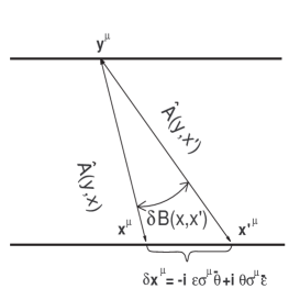
Figure 3: The distinction between two identification prescriptions $\theta$ and $\theta^{\prime}$ leads to a displacement $\delta x^{\mu}=-i\varepsilon^{\alpha}\sigma^{\mu}_{\alpha\dot{\beta}}\bar{\theta}^{\dot{\beta}}+i\theta^{\alpha}\sigma^{\mu}_{\alpha\dot{\beta}}\bar{\varepsilon}^{\dot{\beta}}$

V Acknowledgment

I am very grateful for Doug Singleton and Richard Livine for the comments and fruitful discussion.

Appendix A Calculation of $\delta\hat{B}$ operator

For the proof of Eq. (35) we shall calculate an effect of the $\delta B$ operator on the $\hat{A}$ operator. On the one hand we have

$$\begin{split}&\delta\hat{B}\left(x^{\mu}\rightarrow{x^{\prime}}^{\mu}\right)\hat{A}^{\gamma\delta}\left(y^{\mu},x^{\mu}\right)=\\ &\biggl{(}1+\varepsilon^{\alpha}\frac{\partial}{\partial\theta^{\alpha}}-i\varepsilon^{\alpha}\sigma^{\mu}_{\alpha\dot{\beta}}\bar{\theta}^{\dot{\beta}}\partial_{\mu}-\\ &\bar{\varepsilon}^{\dot{\alpha}}\frac{\partial}{\partial\bar{\theta}^{\dot{\alpha}}}+i\theta^{\alpha}\sigma^{\mu}_{\alpha\dot{\beta}}\bar{\varepsilon}^{\dot{\beta}}\partial_{\mu}\biggl{)}\theta^{\gamma}\theta^{\delta}=\\ &\theta^{\gamma}\theta^{\delta}+\varepsilon^{\gamma}\theta^{\delta}-\varepsilon^{\delta}\theta^{\gamma}\approx\\ &\left(\theta^{\gamma}+\varepsilon^{\gamma}\right)\left(\theta^{\delta}+\varepsilon^{\delta}\right)={\theta^{\prime}}^{\gamma}{\theta^{\prime}}^{\delta}\end{split}$$ (37)

here ${\theta^{\prime}}^{\alpha}=\theta^{\alpha}+\varepsilon^{\alpha}$. On the other hand

$$\begin{split}&\delta\hat{B}\left(x^{\mu}\rightarrow{x^{\prime}}^{\mu}\right)\hat{A}^{\gamma\delta}\left(y^{\mu},x^{\mu}\right)=\\ &\varepsilon^{\gamma\delta}\hat{A}\left(y^{\mu},\delta\hat{B}\left(x^{\mu}\rightarrow{x^{\prime}}^{\mu}\right)x^{\mu}\right)=\\ &\varepsilon^{\gamma\delta}\hat{A}\biggl{(}y^{\mu},\Bigl{(}1+\varepsilon^{\alpha}\frac{\partial}{\partial\theta^{\alpha}}-i\varepsilon^{\alpha}\sigma^{\mu}_{\alpha\dot{\beta}}\bar{\theta}^{\dot{\beta}}\partial_{\mu}-\\ &\bar{\varepsilon}^{\dot{\alpha}}\frac{\partial}{\partial\bar{\theta}^{\dot{\alpha}}}+i\theta^{\alpha}\sigma^{\mu}_{\alpha\dot{\beta}}\bar{\varepsilon}^{\dot{\beta}}\partial_{\mu}\Bigl{)}x^{\mu}\biggl{)}=\\ &\varepsilon^{\gamma\delta}\hat{A}\left(y^{\mu},x^{\mu}-i\varepsilon^{\alpha}\sigma^{\mu}_{\alpha\dot{\beta}}\bar{\theta}^{\dot{\beta}}+i\theta^{\alpha}\sigma^{\mu}_{\alpha\dot{\beta}}\bar{\varepsilon}^{\dot{\beta}}={x^{\prime}}^{\mu}\right)=\\ &\hat{A}^{\gamma\delta}\left(y^{\mu},x^{\mu}+\delta x^{\mu}\right)\end{split}$$ (38)

where

$$\delta x^{\mu}=-i\varepsilon^{\alpha}\sigma^{\mu}_{\alpha\dot{\beta}}\bar{\theta}^{\dot{\beta}}+i\theta^{\alpha}\sigma^{\mu}_{\alpha\dot{\beta}}\bar{\varepsilon}^{\dot{\beta}}.$$ (39)

Therefore we have

$$\hat{A}^{\gamma\delta}\left(y^{\mu},{x^{\prime}}^{\mu}=x^{\mu}+\delta x^{\mu}\right)=$$

$${\theta^{\prime}}^{\gamma}{\theta^{\prime}}^{\delta}=\left(\theta^{\gamma}+\varepsilon^{\gamma}\right)\left(\theta^{\delta}+\varepsilon^{\delta}\right)\approx$$

$$\theta^{\gamma}\theta^{\delta}+\varepsilon^{\gamma}\theta^{\delta}-\varepsilon^{\delta}\theta^{\gamma}.$$ (40)

It means that the operator $\hat{A}^{\gamma\delta}(y^{\mu},{x^{\prime}}^{\mu})$ with the shifted wormhole mouth is equivalent to the change of the Grassmanian coordinate $\theta^{\alpha}\rightarrow{\theta^{\prime}}^{\alpha}$.

References

• (1) C. Misner and J. Wheeler, Ann. of Phys., 2, 525(1957).
• (2) L. Smolin, “Fermions and topology”, gr-qc/9404010.
• (3) Adel Bilal, “Introduction to Supersymmetry”, hep-th/0101055.
• (4) J.Wheeler, Neutrinos, Gravitation and Geometry (Princeton Univ. Press, 1960).
• (5) J. L. Friedman and R. D. Sorkin, Phys. Rev. Lett. 44 (1900) 1100; Gen. Rel and Grav. 14 (1982) 615.
• (6) E. Gozzi, M. Reuter and W. D. Tacker, Phys. Rev., D40, 3363(1989).