Warped compactification on Abelian vortex in six dimensions

Abstract

We consider the possibility of localizing gravity on a Nielsen-Olesen vortex in the context of the Abelian Higgs model. The vortex lives in a six-dimensional space-time with negative bulk cosmological constant. In this model we find a region of the parameter space leading, simultaneously, to warped compactification and to regular space-time geometry. A thin defect limit is studied. Regular solutions describing warped compactifications in the case of higher winding number are also presented.

UNIL-IPT-01-4
hep-th/0104118
April 2001

I Introduction

Topological defects appearing in different field-theoretical models and residing in higher-dimensional space-time can be considered as a prototype of four-dimensional world provided the known particles and gravity are localized on them [1]–[5]. For example, a domain wall solution of a simple $\lambda\phi^{4}$ theory with spontaneous breaking of $\phi\rightarrow-\phi$ symmetry in five-dimensional space-time leads naturally to four-dimensional chiral fermions residing on a domain wall [1] and to four-dimensional gravity [5], if some fine-tuning of a bulk cosmological constant to the domain wall tension is made. A number of “thick” wall solutions in scalar field theory coupled to gravity has been found [6], and the possibility of gravity localization on these walls has been studied.

If a domain wall is replaced by a more complicated topological defect, such as string [7]-[11], monopole [12, 9, 13] or instanton [14, 15] (living, respectively, in 6, 7 or 8 dimensions), the structure of chiral fermionic zero modes, needed for construction of a realistic phenomenology in four dimensions, gets richer. Hence, if the possibility of constructing standard model interactions along these lines from higher dimensions is taken seriously, other fields (scalar, gauge and gravity) must be localized on topological defects as well.

In [11] was shown that a thin string in 6 dimensions could lead to localization of gravity if certain relations between the tension components are satisfied (for even higher-dimensional generalisations see [12, 16]). The aim of the present paper is to provide a field-theoretical realisation of this idea and show that an Abelian Higgs model[17], in which a string defect arises naturally, can lead, at once, to solutions which localize gravity and which have a geometry free of singularities. In the absence of branes a model with an Abelian magnetic field in six dimensions was considered in [18].

The plan of our paper is the following. In Section II the Abelian-Higgs model coupled to six-dimensional Einstein-Hilbert gravity is formulated. In Section III the properties of six-dimensional cylindrically symmetric warped geometries will be discussed in the absence of defects. This is a necessary step for a classification of the solutions in the presence of vortex-type defects. In Section IV the asymptotics of the solutions will be studied both for the metric and for the scalar and gauge fields. Necessary conditions in order to get string solutions will be formulated. Section VI contains numerical examples of the solutions localizing gravity whose parameter space is analyzed in detail. The thin string limit is considered. In Section VII we discuss solutions leading to gravity localization in the case of higher winding numbers and consider regular string solutions which do not localize gravity. Section VIII contains our concluding remarks. In the Appendix useful results concerning the interplay between the thin string limit and the Bogomolnyi limit have been collected.

II Abelian-Higgs model in six dimensions

A Basic equations

The total action of gravitating Abelian Higgs model in six dimensions can be written as

$$S=S_{\rm brane}+S_{\rm grav}~{},$$ (2.1)

where $S_{\rm brane}$ is the gauge-Higgs action and $S_{\rm grav}$ is the six-dimensional generalization of Einstein-Hilbert gravity. More specifically,

$$S_{\rm brane}=\int d^{6}x\sqrt{-G}{\cal L}_{\rm brane},~{}~{}{\cal L}_{\rm brane}=\frac{1}{2}({\cal D}_{A}\phi)^{*}{\cal D}^{A}\phi-\frac{1}{4}F_{AB}F^{AB}-\frac{\lambda}{4}\left(\phi^{*}\phi-v^{2}\right)^{2}~{},$$ (2.2)

where ${\cal D}_{A}=\nabla_{A}-ieA_{A}$ is the gauge covariant derivative, while $\nabla_{A}$ is the generally covariant derivative . In Eq. (2.2), $v$ is the vacuum expectation value of the Higgs field determining the masses of the Higgs and of the gauge boson

$$m_{H}=\sqrt{2\lambda}\,v,\,\,\,m_{V}=e\,v.$$ (2.3)

As usual the bulk action is

$$S_{\rm grav}=-\int d^{6}x\sqrt{-G}\left[\frac{R}{2\chi}+\Lambda\right],$$ (2.4)

where $\Lambda$ is a bulk cosmological constant, $\chi=8\pi G_{6}=8\pi/M_{6}^{4}$ and $M_{6}$ denotes the six-dimensional Planck mass.

From Eqs. (2.1)–(2.4) the coupled system of classical equations of motion can be derived

$$G^{AB}\nabla_{A}\nabla_{B}\phi-e^{2}A_{A}A^{A}\phi-ieA_{A}\partial^{A}\phi-ie\nabla_{A}(A^{A}\phi)+\lambda(\phi^{*}\phi-v^{2})\phi=0~{},$$ (2.5)

$$\nabla_{A}F^{AB}=-e^{2}A^{B}\phi^{*}\phi+\frac{ie}{2}\left(\phi\partial^{B}\phi^{*}-\phi^{*}\partial^{B}\phi\right)~{},$$ (2.6)

$$R_{AB}-\frac{1}{2}G_{AB}R=\chi\left(T_{AB}+\Lambda G_{AB}\right)~{},$$ (2.7)

where

$$T_{AB}=-{\cal L}_{\rm brane}G_{AB}\,+\,\frac{1}{2}\left[({\cal D}_{A}\phi)^{*}{\cal D}_{B}\phi+({\cal D}_{B}\phi)^{*}{\cal D}_{A}\phi\right]-\,F_{AC}{F_{B}}^{C}.$$ (2.8)

We are interested in static string-like solutions of Eqs. (2.5)–(2.7) that depend only on the extra coordinates and thus do not break general covariance along the four physical dimensions. For these solutions a six-dimensional metric is [20, 11]

$$ds^{2}=G_{AB}dx^{A}dx^{B}=M^{2}(\rho)g_{\mu\nu}dx^{\mu}dx^{\nu}-d\rho^{2}-L(\rho)^{2}d\theta^{2},$$ (2.9)

where $\rho$ and $\theta$ are, respectively, the bulk radius and the bulk angle, $g_{\mu\nu}$ is the four-dimensional metric and $M(\rho)$, $L(\rho)$ are the warp factors. The Nielsen-Olesen ansatz for the gauge-Higgs system reads:

$$\phi(\rho,\theta)=vf(\rho)e^{i\,n\,\theta},$$ (2.10)

$$A_{\theta}(\rho,\theta)=\frac{1}{e}[\,n\,-\,P(\rho)]~{},$$ (2.11)

where $n$ is the winding number.

Inserting Eq. (2.11) into Eqs. (2.5)–(2.7) and using the specific form of the metric given in Eq. (2.9), the equations of motion can be written as

$$f^{\prime\prime}+(4m+\ell)f^{\prime}+(1-f^{2})f-\frac{P^{2}}{{\cal L}^{2}}f=0,$$ (2.12)

$$P^{\prime\prime}+(4m-\ell)P^{\prime}-\alpha f^{2}P=0,$$ (2.13)

$$\ell^{\prime}+3m^{\prime}+\ell^{2}+6m^{2}+3\ell m=-\mu-\nu\tau_{0}+\frac{\mu_{\rm ph}}{M^{2}},$$ (2.14)

$$4m^{\prime}+10m^{2}=-\mu-\nu\tau_{\theta}+\frac{2~{}\mu_{\rm ph}}{M^{2}},$$ (2.15)

$$2m\ell+3m^{2}=-\frac{\mu}{2}-\frac{\nu}{2}\tau_{\rho}+\frac{\mu_{\rm ph}}{M^{2}}.$$ (2.16)

The four-dimensional metric $g_{\mu\nu}(\vec{x},t)$ obeys the equation:

$$R^{(4)}_{\mu\nu}-\frac{1}{2}R^{(4)}g_{\mu\nu}=\frac{8\pi}{M_{P}^{2}}\Lambda_{\rm ph}g_{\mu\nu}~{},$$ (2.17)

where the physical cosmological term, $\Lambda_{\rm ph}$, is an arbitrary integration constant and $M_{P}$ is the four-dimensional Planck mass. If $\Lambda_{\rm ph}=0$ we can choose $g_{\mu\nu}=\eta_{\mu\nu}$ where $\eta_{\mu\nu}$ is the Minkowski metric. This will be the case we will be mostly interested in, even though we will often keep the physical cosmological constant, for sake of completeness.

In Eqs. (2.12)–(2.16) the prime denotes the derivation with respect to the rescaled variable

$$x=\,{m_{H}\,\rho\over\sqrt{2}}~{}.$$ (2.18)

The function $L(\rho)$ appearing in the line element of Eq. (2.9) has also been rescaled, namely

$${\cal L}(x)=\frac{m_{H}}{\sqrt{2}}L(\rho).$$ (2.19)

Furthermore, the functions $m(x)$ and $\ell(x)$ are simply

$$m(x)=\frac{d\ln{M(x)}}{dx},\,\,\,\ell(x)=\frac{d\ln{{\cal L}(x)}}{dx}.$$ (2.20)

In Eqs. (2.12)–(2.16) dimensionless parameters have been defined as:

$$\alpha=2\frac{m^{2}_{V}}{m^{2}_{H}},~{}~{}~{}\mu=\frac{2\chi\Lambda}{m^{2}_{H}},~{}~{}~{}\nu=\chi\frac{m^{2}_{H}}{2\lambda},~{}~{}~{}\mu_{\rm ph}=\frac{16\pi\Lambda_{\rm ph}}{M_{P}^{2}m^{2}_{H}}.$$ (2.21)

Within the mentioned conventions the components of the energy-momentum tensor $T_{A}^{B}$ turn out to be

$$\tau_{0}(x) \equiv T_{0}^{0}=T_{i}^{i}=\frac{{f^{\prime}}^{2}}{2}+\frac{1}{4}(f^{2}-1)^{2}+\frac{{P^{\prime}}^{2}}{2\alpha{\cal L}^{2}}+\frac{f^{2}P^{2}}{2{\cal L}^{2}},$$ (2.22)

$$\tau_{\rho}(x) \equiv T_{\rho}^{\rho}=-\frac{{f^{\prime}}^{2}}{2}+\frac{1}{4}(f^{2}-1)^{2}-\frac{{P^{\prime}}^{2}}{2\alpha{\cal L}^{2}}+\frac{f^{2}P^{2}}{2{\cal L}^{2}},$$ (2.23)

$$\tau_{\theta}(x) \equiv T_{\theta}^{\theta}=\frac{{f^{\prime}}^{2}}{2}+\frac{1}{4}(f^{2}-1)^{2}-\frac{{P^{\prime}}^{2}}{2\alpha{\cal L}^{2}}-\frac{f^{2}P^{2}}{2{\cal L}^{2}}.$$ (2.24)

Eqs. (2.12)–(2.13) correspond, respectively, to the equations of motion for the scalar and gauge fields whereas Eqs. (2.14)–(2.16) correspond to the various components of Einstein’s equations. Eqs. (2.14)–(2.15) are truly dynamical since they involve $m^{\prime}(x)$ and $\ell^{\prime}(x)$. Eq. (2.16) connects $m(x)$ and $\ell(x)$ to the first derivatives of the gauge and scalar degrees of freedom and it is, therefore, a constraint. In the following part of the paper $\mu_{\rm ph}=0$ will be assumed.

B Boundary conditions

Regular solutions of the equations of motion can be investigated once the boundary conditions are specified. In order to describe a string-like defect in six dimensions we have to demand that the scalar field reaches, for large $\rho$, its vacuum expectation value, namely $|\phi(\rho)|\rightarrow v$ for $\rho\rightarrow\infty$. In the same limit, the magnetic field should go to zero. Moreover, close to the core of the string both fields should be regular. These requirements can be translated in terms of our rescaled variables as

$$f(0)=0, \lim_{x\rightarrow\infty}f(x)=1,$$ (2.25)

$$P(0)=n, \lim_{x\rightarrow\infty}P(x)=0.$$ (2.26)

The requirement of regular geometry in the core of the string reads:

$$M^{\prime}(0)=0~{},~{}~{}{\cal L}(0)=0~{},~{}~{}{\cal L}^{\prime}(0)=1~{},$$ (2.27)

and one can arbitrarily fix $M(0)=1$.

These conditions listed in Eqs. (2.26)–(2.27) completely specify a solution. Clearly, Eqs. (2.26)–(2.27) do not tell anything about the asymptotics of the metric at large distances from the string and thus a possibility of gravity localization on a defect remains open. The requirement of gravity localization is equivalent to the finiteness of the four dimensional Planck mass,

$$M_{P}^{2}=\frac{4\pi M^{4}_{6}}{m_{H}^{2}}\int dxM^{2}(x){\cal L}(x)<\infty~{},$$ (2.28)

which does not hold in general and requires a fine-tuning of parameters of the model, as it will be discussed.

III Bulk solutions

Outside the core of the string all source terms in Eqs. (2.22)–(2.24) vanish and a general solution to equations

$$\frac{\partial m}{\partial x}+\frac{5}{2}m^{2}+\frac{\mu}{4}=0,$$ (3.1)

$$\ell=-\frac{\mu}{4m}-\frac{3m}{2},$$ (3.2)

can be easily found [20]. We will consider the case $\Lambda\leq 0$ only, since the case of a positive cosmological constant in the bulk was studied in [20]. Defining

$$c=\sqrt{-\frac{\mu}{10}}>0,$$ (3.3)

the solutions of Eqs. (3.2) can be written as

$$m(x)=-c~{}\frac{1-\epsilon\,e^{5cx}}{1+\epsilon e^{5cx}}\,,$$ (3.4)

where $\epsilon$ is an integration constant. Once $m(x)$ is known, $\ell(x)$ can be determined from the second of Eqs. (3.2).

In order to understand whether gravity can be localized on any of those solutions we compute $M$ and ${\cal L}$:

$$M(x)=M_{0}e^{-cx}|1+\epsilon e^{5cx}|^{2\over 5}\,,$$ (3.5)

$${\cal L}(x)={\cal L}_{0}e^{-cx}\frac{|\epsilon e^{5cx}-1|}{|1+\epsilon e^{5cx}|^{3\over 5}}\,.$$ (3.6)

If $\epsilon>0$ or $\epsilon\leq-1$ we have that for $x\rightarrow\infty$ $M\sim{\cal L}\sim e^{cx}$. For this solution the integral in (2.28) diverges and thus gravity cannot be localized.

If $\epsilon=0$ the solution is simply

$$m(x)=\ell(x)=-c,$$ (3.7)

and the warp factors will be exponentially decreasing as a function of the bulk radius:

$$M(x)=M_{0}e^{-cx},\,\,\,$$ (3.8)

$${\cal L}(x)={\cal L}_{0}e^{-cx}.$$ (3.9)

The solution of Eqs. (3.7)–(3.9) leads to gravity localization and to a smooth AdS geometry far from the string core. We also note that a pure positive exponential solution can be derived for $\epsilon\rightarrow\pm\infty$ taking $M_{0}\sim{\rm c}_{1}/|\epsilon|^{2\over 5}$ and ${\cal L}_{0}\sim{\rm c}_{2}/|\epsilon|^{2\over 5}$ where ${\rm c}_{1}$ and ${\rm c}_{2}$ are two arbitrary constants.

If $-1<\epsilon<0$, $M(x_{0})=0$ where $x_{0}=\frac{1}{5c}\log{1/|\epsilon}|$. The geometry is singular at $x=x_{0}$ (see below) and $x<x_{0}$ should be required. In spite of the fact that ${\cal L}$ diverges at $x=x_{0}$, the integral (2.28) defining the four dimensional Planck mass is finite. So, these geometries can be potentially used for a gravity localization, provided the singularity at $x_{0}$ is resolved by some way, e.g. by string theory [19]. These types of singular solutions were discussed in [20] for the case of positive cosmological constant.

Finally, if the bulk cosmological constant is zero, the solutions have a power-law behaviour, namely

$$M(x)\sim x^{\gamma},\,\,\,{\cal L}(x)\sim x^{\delta},$$ (3.10)

with

$$d\gamma+\delta=1,\,\,\,\,d\gamma^{2}+\delta^{2}=1\,,$$ (3.11)

where $d=4$ is the number of dimensions of the metric $g_{\mu\nu}$. These solutions belong to the Kasner class. The Kasner conditions leave open only two possibility: either $\delta=1$ and $\gamma=0$ or $\gamma=2/5$ and $\delta=-3/5$, [the same fractions as in Eqs. (3.6)]. None of them could lead to localization of gravity.

In order to study the singularity structure of the bulk solutions without specifying $\epsilon$, the different curvature invariants may be computed. In the case of warped metrics the Riemann invariant has been calculated in [21]. The explicit form of all the curvature invariants for the metric of Eq. (2.9) is given in [19] and they are:

$$R = 20m^{2}+8m^{\prime}+2\ell^{\prime}+2\ell^{2}+8\ell m,$$ (3.12)

$$R_{AB}R^{AB} = 80m^{4}+20m^{\prime 2}+2\ell^{\prime 2}+2\ell^{4}+64m^{\prime}m^{2}+4\ell^{2}\ell^{\prime}+28m^{2}\ell^{2}$$ (3.13)

$$+ 32m^{3}\ell+8mm^{\prime}\ell+8m^{\prime}\ell^{\prime}+8m^{\prime}\ell^{2}+8m^{2}\ell^{\prime}+8m\ell\ell^{\prime}+8m\ell^{3},$$ (3.14)

$$R_{ABCD}R^{ABCD} = 4\ell^{4}-24m^{4}+8\ell^{2}\ell^{\prime}+4\ell^{\prime 2}+32m^{2}m^{\prime}+16m^{\prime 2},$$ (3.15)

$$C_{ABCD}C^{ABCD} = \frac{12}{5}\left[(m^{\prime}-\ell^{\prime})+\ell(m-\ell)\right]^{2}.$$ (3.16)

Let us first check the regularity properties of the bulk solutions (3.4). The Ricci and scalar curvature invariants are simply constant for any $\epsilon$:

$$R=30c^{2},\,\,\,R_{AB}R^{AB}=150c^{4}.$$ (3.17)

The Riemann and Weyl invariants are

$$R_{ABCD}R^{ABCD}=\frac{-20\,c^{4}\,\left(e^{-20\,c\,x}-12\,e^{-15\,c\,x}\,\epsilon-138\,e^{-10\,c\,x}\,\epsilon^{2}-12\,e^{-5\,c\,x}\,\epsilon^{3}+\epsilon^{4}\right)}{{\left(e^{-5\,c\,x}+\epsilon\right)}^{4}},$$ (3.18)

$$C_{ABCD}C^{ABCD}=\frac{3840\,c^{4}\,e^{-10\,c\,x}\,\epsilon^{2}}{{\left(e^{-5\,c\,x}+\epsilon\right)}^{4}}.$$ (3.19)

From these last two expressions we can see that if $\epsilon>0$ or $\epsilon<-1$ the Weyl and Riemann invariants do not have any pole and thus we have a regular geometry. For $\epsilon=0$ all curvature invariants are constant and we have a six-dimensional AdS space. On the other hand if $-1<\epsilon<0$ both Weyl and Riemann invariants diverge at a finite value of $x$ leading to a singular geometry. The case $\epsilon=-1$ is somewhat specific since a singularity of Kasner type is developed in the origin.

The parameters $\epsilon$, $M_{0}$, ${\cal L}_{0}$ are not fixed for a bulk space solution. If a string-like defects is placed at the origin $x=0$ these constants are no longer arbitrary and are functions of the three parameters of the model, namely, $\epsilon=\epsilon(\alpha,\mu,\nu)$, and so on. An everywhere regular geometry is simultaneously achieved together with gravity localization if the parameters lie on the surface $\epsilon(\alpha,\mu,\nu)=0$.

IV Asymptotics of the solutions

A The asymptotics of the solutions at the origin

The form of the solutions in the vicinity of the core of the vortex can be studied by expressing the metric functions together with the scalar and gauge fields as a power series in $x$, the dimensionless bulk radius. The power series will then be inserted into Eqs. (2.12)–(2.16). Requiring that the series obeys, for $x\rightarrow 0$, the boundary conditions of Eqs. (2.26) the form of the solutions can be determined as a function of the parameters of the model.

Consider, in particular, the case of $n=1$ . In this case asymptotic solutions close to the core can be written as :

$$f(x) \simeq Ax+\left(\frac{2\mu}{3}+\frac{\nu}{6}+\frac{4B^{2}\nu}{3\alpha}+\frac{2A^{2}\nu}{3}-1+2B\right)\frac{A}{8}x^{3},$$ (4.1)

$$P(x) \simeq 1+Bx^{2},$$ (4.2)

$$M(x) \simeq 1+\left(-\frac{\mu}{8}-\frac{\nu}{32}+\frac{\nu B^{2}}{4\alpha}\right)x^{2},$$ (4.3)

$${\cal L}(x) \simeq x+\left[\frac{\mu}{12}+\nu(\frac{1}{48}-\frac{5B^{2}}{6\alpha}-\frac{A^{2}}{6})\right]x^{3}.$$ (4.4)

In Eq. (4.4) $A$ and $B$ are two arbitrary constants which cannot be determined by the local analysis of the equations of motion. These constants are to be found by boundary conditions for $f(x)$ and $P(x)$ at infinity.

For completeness, we give also the limit of the components of the energy-momentum tensor in the vicinity of the origin:

$$\tau_{0}\simeq\biggl{[}\frac{1}{4}+A^{2}+\frac{2\,B^{2}}{\alpha}\biggr{]},$$ (4.5)

$$\tau_{\rho}\simeq\biggl{[}\frac{1}{4}-\frac{2B^{2}}{\alpha}\biggr{]},$$ (4.6)

$$\tau_{\theta}\simeq\biggl{[}\frac{1}{4}-\frac{2B^{2}}{\alpha}\biggr{]}.$$ (4.7)

B The asymptotics of the solutions at infinity

Consider now asymptotics of solutions at large $x$, assuming that the geometry is regular at infinity. This situation can be realized both in the case $\epsilon=0$ [i.e. Eq. (3.7)] and in the case Eq. (3.6) either with $\epsilon>0$ or with $\epsilon<-1$. We can write

$$P(x)=\overline{P}+\delta P(x),$$ (4.8)

$$f(x)=\overline{f}-\delta f(x),$$ (4.9)

where, according to Eqs. (2.26) for $x\gg 1$, $\overline{P}\sim 0$ and $\overline{f}\sim 1$.

First, we will consider the case $\epsilon=0$. From Eq. (2.13) it follows that

$$\delta P^{\prime\prime}-3c\delta P^{\prime}-\alpha\delta P=0,$$ (4.10)

which implies that, for $x\gg 1$

$$\delta P(x)\sim e^{\sigma_{1}x},\,\,\sigma_{1}=\frac{3c}{2}\bigl{[}1\pm\sqrt{1+\frac{4\alpha}{9c^{2}}}\,\,\bigr{]}~{}.$$ (4.11)

If $4\alpha\gg 9c^{2}$ (the limit of small bulk cosmological constant) the solution is compatible with the gauge field decreasing asymptotically as $\delta P\sim e^{-\sqrt{\alpha}x}$ which is the well known flat-space result of the Abelian-Higgs model.

The linearization of the scalar field equation, using a similar procedure, yields

$$\delta f^{\prime\prime}-5c\delta f^{\prime}-2\delta f=0,$$ (4.12)

leading to the solution

$$\delta f(x)\sim e^{\sigma_{2}x},\,\,\,\,\sigma_{2}=\frac{5c}{2}\bigl{[}1\pm\sqrt{1+\frac{8}{25c^{2}}}\,\,\bigr{]}~{}.$$ (4.13)

If $25c^{2}\ll 8$ the perturbed solution goes as $\delta f\sim e^{-\sqrt{2}x}$ which, again, is the flat-space result.

In Eqs. (4.11)–(4.13) a minus sign should be chosen to obtain an exponentially decreasing behaviour. Moreover, linear approximation is only valid if $\sigma_{2}>2\sigma_{1}+2c$, in the opposite case $\delta f\sim\exp(2\sigma_{1}+2c)$.

For $\epsilon\neq 0$ the sign in front of $c$ in equations (4.10,4.12) must be changed, and we get

$$\delta P(x)\sim e^{\sigma_{1}x},\,\,\sigma_{1}=-\frac{3c}{2}\bigl{[}1+\sqrt{1+\frac{4\alpha}{9c^{2}}}\,\,\bigr{]}~{},$$ (4.14)

$$\delta f(x)\sim e^{\sigma_{2}x},\,\,\,\,\sigma_{2}=-\frac{5c}{2}\bigl{[}1+\sqrt{1+\frac{8}{25c^{2}}}\,\,\bigr{]}~{}.$$ (4.15)

The linear approximation is valid if $\sigma_{2}>2\sigma_{1}-2c$, otherwise $\delta f\sim\exp(2\sigma_{1}-2c)$.

C String tensions

In the description of string-like defects in four-dimensions it is useful to study the relations obeyed by the string tensions. Indeed, some particular linear combinations of the string tensions may be related to the Tolman mass per unit length and to the angular deficit of the geometry. These quantities can be used in order to classify the physical properties of the solutions and in order to check if they are effectively asymptotically conical [22].

This analysis is also relevant in our case even though the physical interpretation changes and the specific algebraic relations are different from the well known four-dimensional cases. The components of the string tension are defined as

$$\mu_{i}=\int_{0}^{\infty}dxM^{4}(x){\cal L}(x)\tau_{i}(x).$$ (4.16)

The integrals appearing at the right hand side always converge for solutions with regular geometry, as follows from the results of the previous subsection.

We will show now that for $M(x)\rightarrow 0,~{}~{}{\cal L}(x)\rightarrow 0$ at $x\rightarrow\infty$ (i.e. in the case we are mostly interested in) the constant $B$ in Eq. (4.4) can be analytically determined.

Consider a specific linear combination of Eqs. (2.14)–(2.16), namely

$$2m^{\prime}+4m^{2}+m\ell=-\frac{\mu}{2}-\frac{\nu}{4}\left[\tau_{\rho}+\tau_{\theta}\right],$$ (4.17)

$$\ell^{\prime}+\ell^{2}+4\ell m=-\frac{\mu}{2}-\nu\left[\tau_{0}+\frac{1}{4}\tau_{\rho}-\frac{3}{4}\tau_{\theta}\right].$$ (4.18)

Integrating Eqs. (4.17)–(4.18) from zero to $x_{c}\to\infty$, we get

$$M^{3}(x_{c})M^{\prime}(x_{c}){\cal L}(x_{c})=-\frac{\mu}{2}\int_{0}^{x_{c}}M^{4}{\cal L}dx-\frac{\nu}{4}\left(\mu_{\rho}+\mu_{\theta}\right),$$ (4.19)

$$M(x_{c})^{4}{\cal L}^{\prime}(x_{c})=1-\frac{\mu}{2}\int_{0}^{x_{c}}M^{4}{\cal L}dx-\nu\left(\mu_{0}-\frac{3}{4}\mu_{\theta}+\frac{\mu_{\rho}}{4}\right).$$ (4.20)

In the limit $x_{c}\to\infty$, Eq. (4.19) is the six-dimensional analog of the relation determining the Tolman mass whereas Eq. (4.20) is the generalization of the relation giving the angular deficit. Therefore the following relation must hold:

$$\mu_{0}-\mu_{\theta}=\frac{1}{\nu}\,.$$ (4.21)

This is the fine-tuning relation which has been already found in [11, 12].

Let us note that if $\epsilon\neq 0$ one can use the asymptotics of the metric found in Eq.(3.6) for computation of the left-hand sides of (4.19,4.20). This gives a more general relation,

$$\mu_{0}-\mu_{\theta}=\frac{1}{\nu}(1-10\,c\,\epsilon\,M_{0}^{4}\,{\cal L}_{0})~{}.$$ (4.22)

The extra term vanishes also for $\epsilon\to\pm\infty$ given the scaling behaviour of $M_{0}^{4}\sim|\epsilon|^{-\frac{8}{5}}$ and ${\cal L}_{0}\sim|\epsilon|^{-\frac{2}{5}}$. So, the condition (4.21) is only necessary but not sufficient in order to have solutions leading to gravity localization.

Being an integral relation we can use (4.21) in order to get informations on the behaviour of the solution in the origin. In order to do so, the left hand side of Eq. (4.21) can be directly expressed in terms of the scalar and vector fields

$$\mu_{0}-\mu_{\theta}=\int M^{4}{\cal L}\left[\frac{P^{\prime 2}}{\alpha{\cal L}^{2}}+\frac{f^{2}P^{2}}{{\cal L}^{2}}\right]dx~{}.$$ (4.23)

Using now Eq. (2.13) we arrive at

$$\left(\frac{M^{4}P^{\prime}}{{\cal L}}\right)^{\prime}=\alpha\frac{f^{2}PM^{4}}{\cal L},$$ (4.24)

which can be inserted back into Eq. (4.23). Integrating by parts the obtained relation the term containing ${P^{\prime}}^{2}$ cancels and we arrive at

$$\mu_{0}-\mu_{\theta}=\frac{1}{\alpha}\biggl{(}\left.\frac{P\,P^{\prime}\,M^{4}}{\cal L}\right|_{\infty}-\left.\frac{P\,P^{\prime}\,M^{4}}{\cal L}\right|_{0}\biggr{)}~{}.$$ (4.25)

For the solutions we are interested in the boundary term at infinity vanishes. Using now the asymptotic behaviour for small $x$ of Eqs. (4.4) we obtain, from Eq. (4.25),

$$\mu_{0}-\mu_{\theta}=-\frac{1}{\alpha}\left.\frac{P^{\prime}}{\cal L}\right|_{0}.$$ (4.26)

In this case, from Eq. (4.21) and using Eq. (4.25) we have that

$$-\frac{\nu}{\alpha}\left.\frac{P^{\prime}}{\cal L}\right|_{0}=1\,.$$ (4.27)

According to Eq. (4.4), for $x\rightarrow 0$, $P\sim 1+Bx^{2}$. Using Eq. (4.27) the expression for $B$ can be exactly computed

$$B=-\frac{\alpha}{2\nu}\,.$$ (4.28)

This relation is very helpful for numerical integration of equations of motion performed in the following section.

Finally, we would like to notice that the magnetic field can be expressed as ${\cal B}(\rho)=-P^{\prime}(\rho)/(e\,L(\rho))$. Using now Eq. (4.28) we have that $8\pi{\cal B}(0)=e\,M_{6}^{4}$.

In closing the present Section we want to stress that the results obtained from the analysis of the relations among the tensions are only necessary conditions in order to find $\epsilon=0$ solutions. They are not sufficient because $f^{\prime}(0)\sim A$ still remains undetermined.

V Solutions with localization of gravity

In this Section, a numerical search for solutions that localize gravity will be performed. The general method of integration will be firstly outlined. Secondly, some interesting numerical solutions will be presented as an example. Finally, the scan of the parameter space of the model leading to $\epsilon(\alpha,\mu,\nu)=0$ will be presented.

A Numerical integration

In order to prepare the ground for the numerical integration the system of Eqs. (2.12)–(2.16) can be expressed in a form of a first order non-linear dynamical system. By linearly combining Eqs. (2.12)–(2.16) the following set of equations can be obtained:

$$f^{\prime}=g,$$ (5.1)

$$P^{\prime}=Q,$$ (5.2)

$${\cal L}^{\prime}=l,$$ (5.3)

$$g^{\prime}=-\left(4m+\frac{l}{{\cal L}}\right)g-(1-f^{2})f+\frac{P^{2}}{{\cal L}^{2}}f,$$ (5.4)

$$Q^{\prime}=-\left(4m-\frac{l}{{\cal L}}\right)Q+\alpha Pf^{2},$$ (5.5)

$$m^{\prime}=-\frac{5}{2}m^{2}-\frac{\mu}{4}-\frac{\nu}{4}\left(\frac{g^{2}}{2}+\frac{1}{4}(1-f^{2})^{2}-\frac{Q^{2}}{2\alpha{{\cal L}}^{2}}-\frac{f^{2}P^{2}}{2{\cal L}^{2}}\right),$$ (5.6)

$$l^{\prime}=-\frac{\mu}{4}{{\cal L}}+\frac{3}{2}m^{2}{{\cal L}}-3lm-\frac{\nu{\cal L}}{4}\left(\frac{g^{2}}{2}+\frac{1}{4}(1-f^{2})^{2}+\frac{7Q^{2}}{2\alpha{\cal L}^{2}}+\frac{7f^{2}P^{2}}{2{\cal L}^{2}}\right),$$ (5.7)

$$M^{\prime}=mM.$$ (5.8)

In order to solve this system the shooting method [23] has been employed. In the shooting method a boundary value problem is tackled as a series of Cauchy problem. Using forward integration in $x$ with a specific set of initial conditions, the asymptotic values of the fields are found. If the asymptotic values are different from the boundaries discussed in Eq. (2.26), the integration is performed again with a different set of initial conditions until the correct asymptotic boundary is reached.

The technical problem is twofold. On one hand the shooting method requires that the initial conditions are given in a range of the parameter space sufficiently close to the one admitting $\epsilon(\alpha,\mu,\nu)=0$ solutions. On the other hand, for the scalar and gauge fields the integration is a boundary value problem whereas, for the warp factors, the integration is a Cauchy problem. The shooting method is implemented in such a way that each forward integration is performed by a Runge-Kutta routine. The differences between the obtained values at large $x$ and the boundary values of Eq. (2.26) are considered as functions of the constants $A$ and $B$ appearing in the asymptotic solution in the vicinity of the core. The Newton method [23] is then used in order to find the values of $A$ and $B$ required in order to match the boundaries within the precision of the algorithm.

Therefore, in order to identify a correct set of initial conditions extensive use of backward integrations has been made. Backward integrations have been applied by giving final conditions on warped solutions at large $x$ and by integrating the equations from large to small $x$. This method allowed to identify a set of initial conditions leading to the correct asymptotic boundaries with warped metrics. This idea has also been applied in a different context always involving warped compactification in string inspired models with quadratic curvature corrections [19].

B Some numerical examples

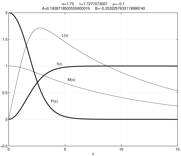
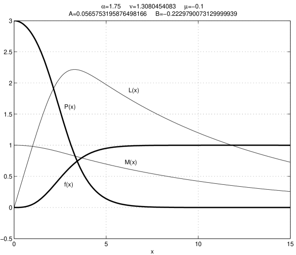
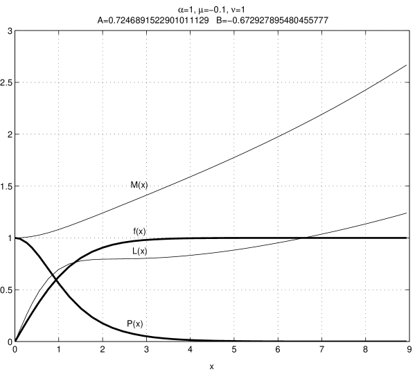
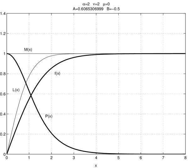
We are now going to give some examples of the numerical integration, see Fig. 1. The values of the scalar and gauge fields are the ones dictated by Eqs. (2.26). At the core of the vortex, the behaviour of the metric and of the other fields follows Eqs. (4.4). For large $x$ the metric functions decay exponentially. The asymptotic behaviour of the metric functions for large $x$ belongs to the class of solutions discussed in Section II for $\epsilon=0$, namely $m\sim\ell\sim-\sqrt{-\mu/10}$.

In the example of Fig. 1, $\alpha=1.16$. The relationship (4.28) is satisfied.

FIG. 1.: A vortex-like solution of the Abelian-Higgs model leading to gravity localization. With the full thick lines we report the behaviour of the scalar and gauge fields whereas with the thin lines the behaviour of the warp factors is illustrated. The same convention will be used throughout the paper.

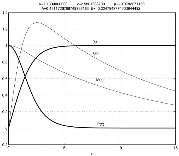
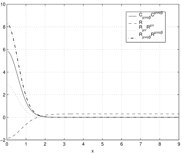
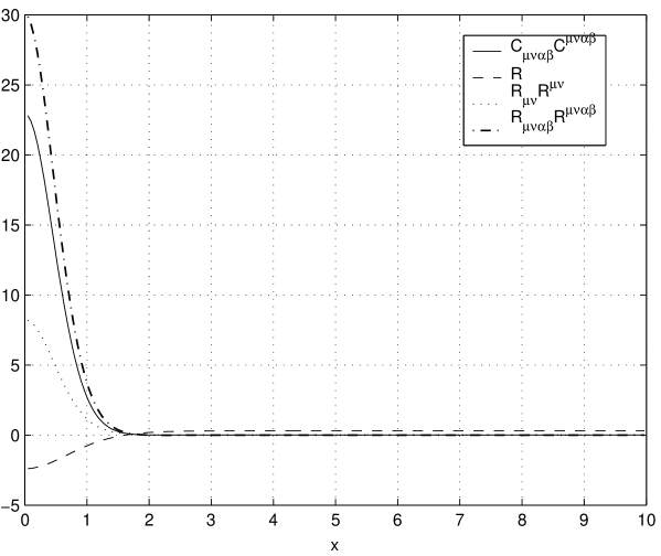
The curvature invariants (scalar curvature, Riemann, Weyl and Ricci invariants) defined in Eqs. (3.12)–(3.16) are plotted in Fig. 2 for the solution illustrated in Fig. 1.

FIG. 2.: The curvature invariants for the solution shown in Fig. 1.

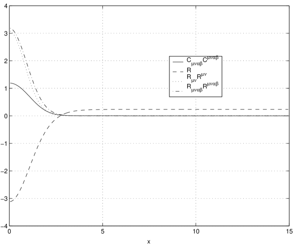
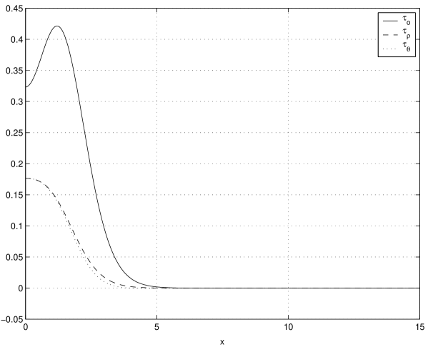
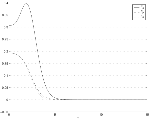
The Riemann and Ricci invariants go asymptotically to a constant which is ${\cal O}(c^{4})$, whereas the scalar curvature goes to a constant ${\cal O}(c^{2})$ as dictated by the asymptotic solutions with $\epsilon=0$ and derived in Eq. (3.7). The Weyl invariant goes to zero since, asymptotically, the space-time is isotropic. Finally it is interesting to check the behaviour of the various components of the energy momentum tensor, which are reported in Fig. 3.

FIG. 3.: The components of the energy momentum tensor of the sources in the case of the numerical solution described in Fig. 1.

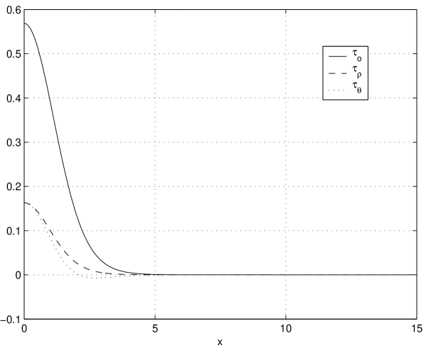
From Fig. 3 we notice that $\tau_{\theta}(x)$ gets negative and it approaches zero from negative values. This is due to the fact that, in $\tau_{\theta}(x)$ the magnetic stresses dominate leading to locally negative pressure.

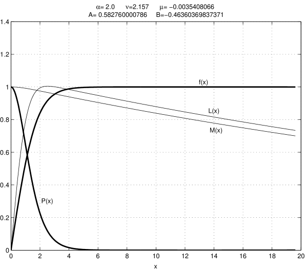
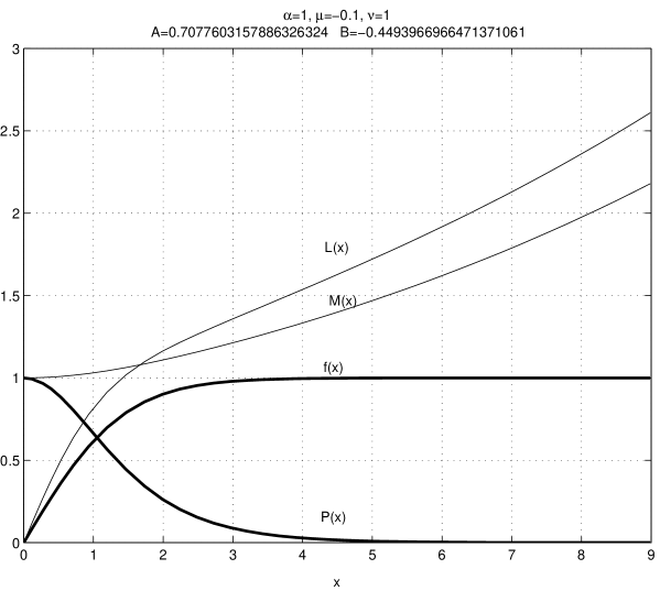
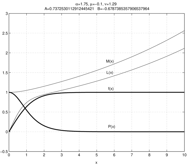
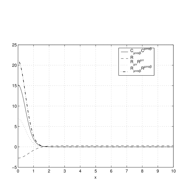
In Fig. 4, we show an example where the exponential damping of the metric is slower than in the case showed in Fig. 1. The reason for this behaviour stems from the fact that the value of the cosmological constant (i.e. the $\mu$ parameter) chosen in Fig. 4 is roughly one order of magnitude smaller than in the case discussed in Fig. 1. The case $\alpha=2$ corresponds to $m_{V}\equiv m_{H}$, i.e. Bogomolnyi limit where the Abelian-Higgs model in four dimensional flat space obeys interesting properties. This limit is discussed in some details in the Appendix.

FIG. 4.: A warped solution is illustrated in the case $\alpha=2$ where $m_{H}=m_{V}$.

To check for the accuracy of numerical integration procedure we consider the constraint equation (2.16) (which was not used in the numerical procedure) that connects $m(x)$ and $\ell(x)$ to the $\tau_{\rho}(x)$ component of the energy-momentum tensor:

$$2m\ell+3m^{2}+\frac{\mu}{2}+\frac{\nu}{2}\tau_{\rho}=0.$$ (5.9)

Inserting the numerical solutions obtained in the present Section into Eq. (5.9) we should find that Eq. (5.9) is numerically satisfied. The accuracy for which Eq. (5.9) is satisfied indicates the accuracy of the integration.

In Fig. 5 we plot the left hand side of Eq. (5.9) for the solution shown in Fig. 1 of this Section.

FIG. 5.: The constraint Eq. (5.9) is illustrated for the case of the solution given in Fig. 1.

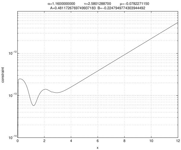
As we can see Eq. (5.9) is satisfied with a precision of $10^{-13}$ in the vicinity of the core and with a precision of $10^{-11}$ for large $x$. For the other solutions similar behaviour can be obtained for the constraint.

C The parameter space of the solutions with gravity localization

Up to this moment, examples of compactifications on a vortex were analyzed. A scan in the parameter space of the solution will now be performed.

In order to achieve this program in a systematic way the procedure is, in short, the following. Suppose that we have already a solution that satisfies all the requirements (for example, the one in Fig. 1 or 4). It can be found by a procedure of backward integration discussed above. Then one of the three parameters among $\alpha$, $\nu$ and $\mu$ is kept fixed, a second is changed by small steps and the third one is tuned to the first two by requiring that

$$\ell(x)+\sqrt{\frac{-\mu}{10}}=0,$$ (5.10)

$$m(x)+\sqrt{\frac{-\mu}{10}}=0,$$ (5.11)

are satisfied for large $x$. The zeroes of Eq. (5.11) are found by means of a simple bisection method [23].

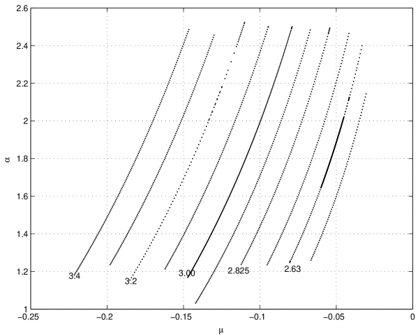
Using this procedure a scan of the parameter space of the model has been performed. Let us start by discussing the scan in the $(\mu,\alpha)$ plane at constant $\nu$. The results of the study are shown in Fig. 6.

FIG. 6.: We illustrate the variation of $(\alpha,\mu)$ for fixed $\nu$. Along each line in this plane the numerical $\nu$ is constant and it is given by the numerical values reported at the bottom of the curves.

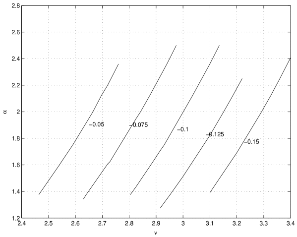
The same type of procedure can be carried on in the case of fixed $\mu$. As a result we will get the $(\alpha,\nu)$ projection of the parameter space of the solution. This result is presented in Fig. 7.

FIG. 7.: The $(\alpha,\nu)$ projection of the parameter space of the warped solution is illustrated. The curves correspond to lines of constant $\mu$.

Finally we can also investigate the $(\mu,\nu)$ plane at for fixed $\alpha$. In this case the results of our study are shown in Fig. 8.

FIG. 8.: We report the variation of $(\mu,\nu)$ for fixed $\alpha$. As in the previous figures the numerical values represent the values of $\alpha$ which is kept constant along each curve.

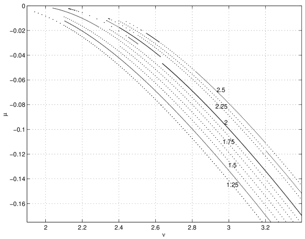
In Fig. 8 we can notice that the limit $\mu\rightarrow 0$ at $\alpha=2$ implies that $\nu\rightarrow 2$. This can be shown analytically, see Appendix.

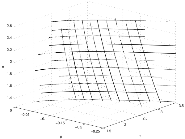
Finally, in order to give a visual feeling of the fine-tuning surface we can present a three-dimensional plot in the $(\alpha,\mu,\nu)$ plane. This surface is illustrated in Fig. 9. The points on this surface defines a fine-tuned solution of the types presented in Fig. 1 and Fig. 4.

FIG. 9.: We illustrate the three-dimensional picture of the fine-tuning surface in the $(\alpha,\mu,\nu)$ plane. The points on the surface correspond to warped solutions obeying the boundaries of Eq. (2.26).

D The thin-string limit

The thin string limit was used for gravity localization in [11]. In this limit the energy density of the vortex gets more and more localized in the origin while the exponential damping of the warp factors gets milder as in Fig. 4. Here we will show how the thin-string limit implemented in the Abelian Higgs model.

The main idea of a thin string limit is to replace the real thick string made of the scalar and gauge fields by a thin gravitating object characterized by three different string tensions defined in Eq. (4.16). Then the parameters of the metric outside the string $M_{0},~{}{\cal L}_{0},~{}\epsilon$ and four-dimensional Planck constant are related in a simple way to the string tensions [i.e. $\mu_{0},\mu_{\rho}$ and $\mu_{\theta}$], to the six-dimensional Planck constant, and to the bulk cosmological constant. These relationships were worked out for the gravity localizing solution in Ref.[11] (see also [24]), and they can be reproduced as well from Eqs. (4.19)–(4.20) assuming that $c\ll 1$, which is a condition for a thin string limit in dimensionless variables.

Here we will write somewhat more general equations valid also for $\epsilon\geq 0$ or $\epsilon<-1$ that lead to regular geometry at infinity. For $c\ll 1$ the integrals and limits $x_{c}\to\infty$ can be explicitly taken, and one gets

$$M_{0}^{4}{\cal L}_{0}c(1-\epsilon)^{2}+{\cal O}(c^{2})=-\frac{\nu}{4}\left(\mu_{\rho}+\mu_{\theta}\right)~{},$$ (5.12)

$$M_{0}^{4}{\cal L}_{0}c(1+8\epsilon+\epsilon^{2})+{\cal O}(c^{2})=1-\nu\left(\mu_{0}-\frac{3}{4}\mu_{\theta}+\frac{\mu_{\rho}}{4}\right)~{}.$$ (5.13)

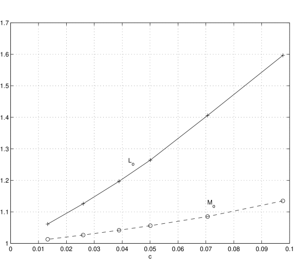
As the numerical analysis shows (see also analytic discussion in Appendix), in the limit $c\to 0$ the parameters $M_{0}$ and ${\cal L}_{0}$ go to some non-zero constants (see, e.g. Fig. 10). Then it is clear from Eqs. (5.12)–(5.13), that the combination $\mu_{\rho}+\mu_{\theta}$ scales as ${\cal O}(c)$. In fact, as shown in [24], this feature has a more general character and it is not related to the specific form of the Lagrangian of the Abelian-Higgs model.

FIG. 10.: The variation of $M_{0}$ and ${\cal L}_{0}$ as a function of $c$ for $\alpha=2$.

It is interesting to ask the question whether a thin string limit $c\ll 1$ can be organised in a way that :
(i) the four-dimensional Planck scale is a finite constant;
(ii) corrections to the four-dimensional Newton law stay small;
(iii) classical gravity is applicable in the bulk;
and, eventually
(iv) classical gravity is applicable in the core of the string.

In order to answer these questions let us go back to the dimension-full parameters of the model. They are

$$\Lambda\equiv M_{\Lambda}^{6},\,\,\,M_{6},\,\,\,m_{H},\,\,\,\lambda,\,\,\,e^{2}.$$ (5.14)

The other parameters can be expressed as a function of the previous ones since we know that, for instance,

$$\alpha=\frac{e^{2}}{\lambda}=2\frac{m_{V}^{2}}{m_{H}^{2}}~{}.$$ (5.15)

In order to have only two scales in the problem, we can then take $\alpha$ to be fixed to given value (for instance $\alpha=2$). Once $\alpha$ has been fixed, we can see if, in the limit $c\ll 1$, the requirements (i)–(iv) can be satisfied. In order to solve the problem, we should know the values of $M_{0}$ and $L_{0}$ defined in Eq. (3.7) in the thin string limit and also the limit of parameter $\nu$. An analytic discussion of these questions is contained in Appendix. Here we simply state the results. In the limit $c\rightarrow 0$ and for $\alpha=2$, $\nu=2$ [see Fig. 8], and $M_{0}={\cal L}_{0}=1$ [see Fig. 10].

(i) The four-dimensional Planck mass

$$M_{P}^{2}=\frac{4\pi M^{4}_{6}}{m_{H}^{2}}\int dxM^{2}(x){\cal L}(x)$$ (5.16)

for small $c$ and $\alpha=2$ is simply

$$M_{P}^{2}=\frac{\sqrt{10\pi}}{3}\frac{M^{6}_{6}}{m_{H}\sqrt{|\Lambda|}}~{},$$ (5.17)

which must be equal to $[1.22\times 10^{19}{\rm GeV}]^{2}$.

(ii) Corrections to 4d gravity were computed in [11] and are given by ${4\over 3\pi}(r_{0}/r)^{3}$. They are known to be small at the distances smaller than $0.2$ mm [25] and thus we require

$$r_{0}=\frac{0.2~{}{\rm mm}}{\xi}~{},~{}~{}\xi>1~{}.$$ (5.18)

(iii) To parameterize the Planck constant in the bulk, we write

$$M_{6}=\eta\,10^{3}{\rm GeV}~{}.$$ (5.19)

The choice of $\eta\sim 1$ makes the fundamental Planck scale to be of the order of the weak scale and may potentially lead to the solution of the gauge hierarchy problem [26]. To satisfy the third requirement, we must have the curvature in the bulk to be smaller than $M_{6}^{2}$, i.e. $M_{\Lambda}<M_{6}$.

(iv) If we require the validity of gravity on the string we should demand that the (quadratic) curvature invariants of the solution are always much smaller than $M_{6}^{4}$. In the small $x$ limit the curvature invariants are

$$R^{2}\sim m^{4}_{H}\,\frac{\,{\left(-8\,\alpha+\nu\,\left(4\,\mu+\nu\right)\right)}^{2}}{4\,{\nu}^{2}},$$ (5.20)

$$R_{AB}R^{AB}\sim m^{4}_{H}\,\frac{5\,{\left(-8\,\alpha+\nu\,\left(4\,\mu+\nu\right)\right)}^{2}}{64\,{\nu}^{2}},$$ (5.21)

$$R_{ABCD}R^{ABCD}\sim m^{4}_{H}\,\frac{{\left(-8\,\alpha+\nu\,\left(4\,\mu+\nu\right)\right)}^{2}}{16\,{\nu}^{2}},$$ (5.22)

$$C_{ABCD}C^{ABCD}\sim m_{H}^{4}\,\frac{3\,{\left(-8\,\alpha+\nu\,\left(4\,\mu+\nu\right)\right)}^{2}}{320\,{\nu}^{2}}.$$ (5.23)

So, we find that this requirement is satisfied if

$$\frac{m_{H}}{M_{6}}\ll 1~{}.$$ (5.24)

In numbers, the thin string limit $c\ll 1$ implies

$$c\simeq 70\times\frac{\xi^{2}}{\eta^{4}}\ll 1~{},$$ (5.25)

the third condition requires

$$\frac{\eta}{\xi}\gg 6\times 10^{-16},$$ (5.26)

and the ratio $\frac{m_{H}}{M_{6}}$ essential for the requirement (iv) is

$$\frac{m_{H}}{M_{6}}\simeq 2\times 10^{-17}\frac{\eta^{3}}{\xi}~{}.$$ (5.27)

One can see that all these conditions can be satisfied in a wide range of the parameters of the model. For example, the hierarchy $M_{6}\ll M_{P}$ can be easily achieved for $\eta\sim 10,~{}~{}\xi\sim 1$.

If the limit $c\to 0$ is taken in mathematical sense, it is impossible to satisfy all four conditions, because the curvature of the space inside the string diverges. However, the first three conditions can be satisfied, if the parameters of the model scale as:

$$m_{H}=E\biggl{(}{1\over c}\biggr{)}^{\beta}~{},$$ (5.28)

$$\Lambda=E^{6}\biggl{(}{1\over c}\biggr{)}^{4\beta-3},$$ (5.29)

$$M_{6}^{4}=E^{4}\biggl{(}{1\over c}\biggr{)}^{2\beta-1},$$ (5.30)

$$\lambda=E^{-2}\biggl{(}{1\over c}\biggr{)},$$ (5.31)

with $1<\beta<{3\over 2}$ and $E$ being an arbitrary energy scale.

VI Extensions

A Higher windings

The parameter space of the solutions discussed in the previous sections has been derived in the case $n=1$. It is also possible to discuss the case of higher windings $n\geq 2$. The study of these cases can be performed using the same techniques discussed in the case of $n=1$. There are obvious differences in the asymptotics of the solutions. For the gauge field we have to require that $P(0)=n$. This imposes a different asymptotic solution in the core, namely

$$f(x) = Ax^{n}+Fx^{n+2},$$ (6.1)

$$P(x) = n+Bx^{2},$$ (6.2)

$$M(x) = 1+Cx^{2},$$ (6.3)

$${\cal L}(x) = x+Dx^{3}.$$ (6.4)

For $n\geq 2$, we find:

$$C = -\frac{\mu}{8}-\frac{\nu}{32}+\frac{B^{2}\nu}{4\alpha},$$ (6.5)

$$D = \frac{\mu}{12}+\frac{\nu}{48}-\frac{5B^{2}}{6\alpha},$$ (6.6)

$$F = A\left(-1+2Bn-\frac{B^{2}\nu}{3\alpha}(n-5)+\frac{5n-1}{6}\left(\mu+\frac{\nu}{4}\right)\right).$$ (6.7)

With these solutions it is possible to integrate the system by repeating the same procedure discussed in the case $n=1$.

Since the winding number determines the value of the gauge field at the origin the relations among the string tensions will also be modified. In particular, Eq. (4.26) becomes, in the case of $n\geq 2$,

$$\mu_{0}-\mu_{\theta}=-\frac{n}{\alpha}\left.\frac{P^{\prime}}{\cal L}\right|_{0},$$ (6.8)

which implies that $B$, appearing in Eqs. (6.1)–(6.4), is now

$$B=-\frac{\alpha}{2n\nu}~{}.$$ (6.9)

As in the case $n=1$ the tuning of the string tensions expressed in terms of $B$ is only necessary (but not sufficient) in order to get solutions which lead to gravity localization. Thus, as in the case $n=1$, $A$ should be again tuned.

FIG. 11.: A solution leading to gravity localization in the case of winding $n=2$ is illustrated.

In Fig. 11 we illustrate an example of regular solutions with $n=2$. The components of the energy-momentum tensor corresponding to the solution of Fig. 11 are reported in Fig. 12.

FIG. 12.: The components of the energy-momentum tensor computed from the solution of Fig. 11 are illustrated.

In Fig. 13 a solution which localizes gravity is reported in the case $n=3$.

FIG. 13.: An example of solution with $n=3$.

In Fig. 14 the components of the energy-momentum tensor are reported for the solution illustrated in Fig. 13.

FIG. 14.: The components of the energy-momentum tensor in the case of the solution reported in Fig. 13.

The solutions illustrated in Fig. 11 and 13 lead to regular geometry since all the curvature invariants are finite for any $x$. As in the case $n=1$ a full scan of the parameter space could be performed following the same procedure outlined in the body of the paper. It is interesting to speculate that these solutions may have some implications in models trying to explain the origin of families in a higher dimensional context [27]. It would then be of some interest to study, in the context of solutions with higher windings, the structure and localization of the fermionic zero modes.

B String solutions without localization of gravity

The examples discussed up to this point illustrated mainly solutions whose warp factors decrease at infinity. In this section we will give some examples of solutions with the opposite type of behaviour.

In Fig. 15 we show a regular solution of Eqs. (2.12)–(2.16) where the warp factors increase at large distance from the core. The parameters of Fig. 15 are $\alpha=1$, $\nu=1$, $\mu=-0.1$.

FIG. 15.: We illustrate and anti-warped solution with parameters $\alpha=1$, $\nu=1$ and $\mu=-0.1$.

In the solution of Fig. 15 Eq. (4.28) does not hold. From Eq. (4.28) we should have $B=-0.5$ whereas, for Fig. 15 $B\neq-0.5$. In this sense the solution is not fine-tuned. In Fig. 16 we plot the curvature invariants pertaining to the solution of Fig. 15.

FIG. 16.: The curvature invariants for the solution shown in Fig. 15.

For large $x$ the asymptotic behaviour illustrated in Fig. 15 can be related to the solutions given in Eq. (3.4).

It is interesting that the same values of $\alpha$, $\nu$ and $\mu$ selected for the solution of Fig. 15 admit a physically distinct extra solution. It is shown in Fig. 17 and the related curvature invariants are illustrated in Fig. 18.

FIG. 17.: The parameters of the solution discussed in this plot are the same of Fig. 15 but with different $A$ and $B$. The curvature in the origin is larger than in the case of Fig. 16.

FIG. 18.: The curvature invariants for the solution of Fig. 17.

We will not attempt here a full classification of the solutions. We can notice, however, that the solutions illustrated in Fig. 15 and Fig. 17 can be distinguished (in a coordinate independent fashion) from the behaviour of the curvature invariants in the origin. As we can see from Figs. 16 and 18 the solution of Fig. 17 leads to larger curvature invariants in the origin.

Finally we want to demonstrate that the tuning of the string tensions as implied by Eq. (4.28) is not a sufficient condition in order to obtain solutions with localization of gravity. In Fig. 19 and Fig. 20 we illustrated a regular solution whose parameters are given by $\alpha=1.75$, $\nu=1.29$ and $\mu=-0.1$ and tensions fine tuned according to Eq. (4.28). Nevertheless, the metric increases at infinity.

FIG. 19.: We illustrate a solution where the string tensions have been fine-tuned according to Eq. (4.28) but with the metric growing at infinity.

FIG. 20.: The curvature invariants associated with the solution of Fig. 19.

Asymptotically for large $x$ the solution of Fig. 19 are the ones of Eq. (3.4) with $\epsilon\to\infty$.

VII Concluding remarks

In this paper we discussed the possibility of obtaining solutions which localize gravity in six-dimensions. The source of the gravitational field has been assumed to be a generalized version of the Nielsen-Olesen vortex living in the two-dimensional transverse space.

We show that the localization of gravity is possible on a “thick” string and found a fine-tuning condition leading to a set of physically interesting solutions. Since the geometries described in this paper are regular (i.e. curvature singularities are absent) gravity can be described in classical terms both in the bulk and on the vortex. We studied a thin string limit and identified the choice of parameters that may potentially lead to a solution to the gauge hierarchy problem.

Various questions are still open. Our explicit solutions couple together scalar, tensor and gauge degrees of freedom. Therefore they represent an ideal framework where the localization of fields of various spin can be explicitly analyzed in a completely regular geometry. There are also open questions concerning higher windings. It has been shown that also for higher windings there are solutions which localize gravity. It would be natural to ask if these solutions are as stable as the ones obtained in the case of the lowest winding. Finally, since the geometries discussed in this paper are completely regular (in a technical sense) it is interesting to understand their stability against first order (quadratic) corrections to the Einstein-Hilbert action [19] (which may naturally arise in a string theoretical context).

We thank P. Tinyakov and K. Zuleta for discussions. This work was supported by the FNRS grants no. 21-55560.98, 7SUPJ62239 and by the Tomalla Foundation.

A The Bogomolnyi limit

In this appendix we show analytically that for the case $\alpha=2$ (the Bogomolnyi limit [28]) the following limits hold:

$$\lim_{c\rightarrow 0}\nu(c)=2~{},$$ (A.1)

$$\lim_{c\rightarrow 0}M_{0}(c)=1~{},$$ (A.2)

and

$$\lim_{c\rightarrow 0}{\cal L}_{0}(c)=1~{},$$ (A.3)

if the string tensions are tuned according to Eqs. (4.25)–(4.26). The numerical solution for the Bogomolnyi limit is shown in Fig. 21.

FIG. 21.: A solution in the Bogomolnyi limit for $c\ll 1$.

In the Bogomolnyi limit and for $c=0$ the equations of motion for the gauge and scalar fields reduce to a coupled set of first order non-linear differential equations which can be written as

$${\cal L}\,f^{\prime}=f\,P,$$ (A.4)

$$\frac{P^{\prime}}{\cal L}=f^{2}-1.$$ (A.5)

If we insert Eqs. (A.5) into Eqs. (2.22)-(2.24) we obtain that

$$\tau_{\rho}(x)=\tau_{\theta}(x)=0.$$ (A.6)

The equation for $M$ becomes then

$$4m^{\prime}+10m^{2}=-\mu.$$ (A.7)

The limit $c\rightarrow 0$ implies that $\mu\rightarrow 0$. From Eq. (A.7) the only (regular) solution respecting the boundary conditions at the origin is then $M(x)=M_{0}=1$. Thus, this proves Eq. (A.2).

Since $\tau_{\rho}(x)=0$, from Eq. (4.7) we get $B^{2}=\alpha/8=1/4$ and from Eq. (4.28) $\nu=2$. Thus, this proves that, once the string tensions are tuned, Eq. (A.1) is valid.

Now, the difference of Eqs. (2.14) and (2.15) yields,

$$(M^{3}M^{\prime}L)^{\prime}-(M^{4}L^{\prime})^{\prime}=\nu M^{4}L(f_{o}-f_{\theta})~{}.$$ (A.8)

By using for $P(x)$ Eq. (2.13) we have:

$$M^{4}L(f_{o}-f_{\theta})=\left(\frac{PP^{\prime}M^{4}}{\alpha L}\right)^{\prime}~{}.$$ (A.9)

Thus all terms in (A.8) are total derivatives; integrating both sides from 0 to $x$ we obtain

$$m-\ell=\frac{\nu}{\alpha}\frac{PP^{\prime}}{L^{2}}-\left(1+\frac{\nu}{\alpha}n\left.\frac{P^{\prime}}{L}\right|_{0}\right)\frac{M_{o}^{4}}{M^{4}L}~{},$$ (A.10)

where $M_{o}$ is the value of $M$ on the core of the string and $n$ is the winding. In the case of fine-tuned solution, according to Eq. (4.28), the last term in Eq. (A.10) vanishes. Since we just showed that in the limit $\alpha\to 2$ we have $\nu\to 2$ and $M\to 1$, from Eq. (A.10) we get

$$LL^{\prime}=-PP^{\prime}~{},$$ (A.11)

which gives, after integration over $x$,

$$L^{2}=1-P^{2}~{},$$ (A.12)

where we used the fact that $P(0)=1$. This proves (A.3), because $P(x)\to 0$ for $x\to\infty$.

REFERENCES

- [1] V. Rubakov and M. Shaposhnikov, Phys. Lett. B 125 (1983) 136.
- [2] K. Akama, in Proceedings of the Symposium on Gauge Theory and Gravitation, Nara, Japan, eds. K. Kikkawa, N. Nakanishi and H. Nariai, (Springer-Verlag, 1983), [hep-th/0001113].
- [3] M. Visser, Phys. Lett. B 159 (1985) 22.
- [4] G. Dvali and M. Shifman, Phys. Lett. B 396 (1997) 64 [Erratum-ibid. B 407 (1997) 64].
- [5] L. Randall and R. Sundrum, Phys. Rev. Lett. 83 (1999) 3370.
- [6] M. Gremm, Phys. Lett. B 478 (2000) 434; A. Kehagias, and K. Tamvakis hep-th/0010112.
- [7] A. G. Cohen and D. B. Kaplan, Phys. Lett. B 470 (1999) 52;
- [8] A. Chodos and E. Poppitz, Phys. Lett. B 471 (1999) 119;
- [9] I. Olasagasti and A. Vilenkin, Phys. Rev. D 62 (2000) 044014;
- [10] R. Gregory, Phys. Rev. Lett. 84 (2000) 2564.
- [11] T. Gherghetta and M. Shaposhnikov, Phys.Rev.Lett. 85 (2000) 240.
- [12] T. Gherghetta, E. Roessl, M. Shaposhnikov, Phys.Lett.B 491 (2000) 353.
- [13] G. Dvali, hep-th/0004057.
- [14] S. Randjbar-Daemi, A. Salam and J. Strathdee, Phys. Lett. B 132 (1983) 56.
- [15] S. Randjbar-Daemi and M. Shaposhnikov, Phys. Lett. B 492 (2000) 361.
- [16] S. Randjbar-Daemi and M. Shaposhnikov, Phys. Lett. B 491 (2000) 329.
- [17] H.B. Nielsen and P. Olesen, Nucl. Phys.B 61 (1973) 45.
- [18] G. W. Gibbons and D. L. Wiltshire, Nucl. Phys. B 287 (1987) 717.
- [19] M. Giovannini, Phys. Rev. D 63 (2001) 064011; Phys.Rev.D 63 (2001) 085005.
- [20] V. Rubakov and M. Shaposhnikov, Phys. Lett. B 125 (1983) 139.
- [21] S. Randjbar-Daemi and C. Wetterich, Phys. Lett. B 166 (1986) 65.
-
[22]
Y. Brihaye and
M. Lubo Phys.Rev.D 62 (2000) 085004;
M. Christensen, A.L. Larsen and Y. Verbin, Phys. Rev. D 60 (1999);
Y. Verbin, Phys.Rev.D 59 (1999) 105015. - [23] W. H. Press, S. A. Teukolsky, W. T. Vettrling, B. P. Flannery, Numerical Recipies in Fortran 77, second edition, (Cambridge University Press, Cambridge United Kingdom, 1995).
- [24] P. Tinyakov and K. Zuleta, hep-th/0103062.
- [25] C. D. Hoyle et al., Phys. Rev. Lett. 86, 1418 (2001).
[26]
N. Arkani-Hamed, S. Dimopoulos, G. Dvali, Phys.Lett.B 429 (1998)
263;
I. Antoniadis, N. Arkani-Hamed, S. Dimopoulos, G. Dvali, Phys.Lett.B 436 (1998) 257;
I. Antoniadis, S. Dimopoulos, G. Dvali Nucl.Phys.B 516 (1998) 70. - [27] M.V. Libanov and S.V. Troitsky Nucl. Phys. B 599 (2001) 319; J. M. Frere, M.V. Libanov and S.V. Troitsky, hep-ph/0012306.
- [28] E. B. Bogomol’nyi, Sov. J. Nucl. Phys. 24 (1976) 449 [ Yad. Fiz. 24 (1976) 861].