Comments on the renormalizability of the Broken Symmetry Phase in Noncommutative Scalar Field Theory

Abstract

We study the noncommutative $\phi^{4}$ theory with spontaneously broken global O(2) symmetry in 4 dimensions. We demonstrate the renormalizability at one loop. This does not require any choice of ordering of the fields in the interaction terms. It involves regulating the ultraviolet and infrared divergences in a manner consistent with the Ward identities.

I introduction

Noncommutative spacetimes have been studied intensively over the last few years [1][2][3]. The fact that they occur as low energy limit of String Theory when a constant $B_{\mu\nu}$ background is turned on makes the subject even more interesting [3]. A perturbative study of $\phi^{4}$ field theory revealed an intriguing transmutation of some UV divergences into IR divergences [5]. This is very reminiscent of what happens in string perturbation theory where the world sheet duality or modular invariance maps the UV region into the IR region. This is the origin of the well known fact that there are no UV divergences in String Theory.

In the light of the above remarks it is natural to wonder about perturbative renormalizability of the noncommutative $\phi^{4}$ theory. It was argued in [5] that the UV divergences that continue to arise in the theory are from Planar graphs [4] and are exactly of the same form as in the commutative theory and hence can be renormalized away. The UV divergences from the non-planar graphs are, on the face of it, more severe. However they turn into IR divergences in an intriguing way and are UV finite. The non-planar graphs therefore do not threaten the renormalizability of the theory. Various other aspects of Noncommutative field theories have been studied in [6-34].

Issues concerning the renormalizability of theories with global O(N) symmetry, in the large N limit have been addressed in [15],[34]. One can also study these issues in theories with global O(2) symmetry, in their broken/unbroken phases. In commutative theories if the theory is renormalizable in the unbroken phase it is trivially renormalizable in the broken phase. The Ward Identities guarantee this as also the masslessness of the Goldstone Bosons, to all orders in perturbation theory. However it was found in [32] that in the noncommutative O(2) theory there seems to be a violation of these identities at the one loop level. The crucial point being that the counterterm that renormalized the $\sigma$-tadpole divergence could not remove the divergences in the $\pi$-$\pi$ two point function. It was also found [33],[32] that for a particular choice of ordering of fields in the $\phi^{4}$ couplings, the theory is renormalizable.

Given that both the path integral measure and the action of the noncommutative theory have global O(2) symmetry one would expect this symmetry to hold at one loop (in fact to all orders). We investigate this in this paper. We show that the apparent violation of the Ward identities can be traced to the dropping of surface terms in the effective action. These are UV divergent surface terms. If one modifies the prescription to keep these terms, the broken theory is renormalizable. The crucial point is to keep an infrared regulator while the continuum limit ($\Lambda\rightarrow\infty$) is taken for all the processes in the theory. This prescription allows one to maintain O(2) symmetry in the UV divergent terms. However the infrared divergences make it difficult to use the Ward Identities for the two point function in the limit $p\rightarrow 0$ (which is required to establish the masslessness of the pion).

This paper is organised as follows. In section II we describe the basic problem in the context of an O(2) model and point out the reason for it and suggest a resolution. In section III as a preliminary step we calculate one loop graphs in the symmetric phase and discuss the Ward Identity. In section IV as a next step we expand one of the fields about a background value, but only in external legs i.e. masses are kept at the symmetric (tachyonic) value. We show that one can preserve the Ward Identity if we set the momentum of the background to zero only at the end of the loop calculations. In section V we consider the broken phase of the theory where the masses in the loop are the physical (tree-level) masses and describe a prescription that allows the Ward Identities to be maintained (at one loop). We give our conclusions in section VI.

II Ward Identities and outline of the prescription

In this section we derive the relevant Ward Identities for the symmetric as well as for the broken phases and show in the following sections that the Ward Identities hold for one loop calculations.

Consider the global O(2) invariant action $S[\phi]$,

$$Z[J] = \int{\cal D}\phi_{1}{\cal D}\phi_{2}e^{i[S[\phi]+\int d^{4}x\phi_{i}J_{i}]}$$ (1)

$$[i = 1,2]$$ (2)

The action is invariant under the following transformation,

$$\phi^{i}\rightarrow\phi^{i}+\epsilon^{ij}\phi^{j}$$ (3)

where $\epsilon^{ij}$ is an infinitesimal parameter antisymmetric in the $i$, $j$ indices. So is the measure defined by,

$$\int{\cal D}\phi e^{[-\frac{1}{2}\int d^{4}x\phi*\phi]}=\int{\cal D}\phi e^{[-\frac{1}{2}\int d^{4}x\phi^{2}]}=1$$ (4)

Where, the $*$-product is defined by,

$$(\phi_{1}*\phi_{2})(x)=e^{\frac{i}{2}\theta^{\mu\nu}\partial_{\mu}^{y}\partial_{\nu}^{z}}\phi_{1}(y)\phi_{2}(z)\mid_{y=z=x}$$ (5)

$\theta^{\mu\nu}$ is real and antisymmetric. We have used the fact [5] that in quadratic terms the $*$-product can be replaced by an ordinary product. Since action and the measure are invariant under this transformation, the generating functional satisfies,

$$Z[J]=Z[J+\epsilon J]$$ (6)

or,

$$\epsilon^{ij}J^{i}\frac{\delta Z}{\delta J^{j}}=0$$ (7)

Using the definition of quantum effective action,

$$\Gamma[\phi]=-\int d^{4}x\phi^{i}(x)J^{i}(x)+W[J]$$ (8)

$$W[J]=-ilnZ[J]$$ (9)

We have the following set of Ward Identities,

$$\phi_{1}\frac{\delta\Gamma}{\delta\phi_{2}} = \phi_{2}\frac{\delta\Gamma}{\delta\phi_{1}}$$ (10)

$$\frac{\delta^{2}\Gamma}{\delta\phi_{1}^{2}}\mid_{\phi_{1}=\phi_{2}=0} = \frac{\delta^{2}\Gamma}{\delta\phi_{2}^{2}}\mid_{\phi_{1}=\phi_{2}=0}$$ (11)

$$\frac{\delta^{4}\Gamma}{\delta\phi_{1}^{4}}\mid_{\phi_{1}=\phi_{2}=0} = 3\frac{\delta^{4}\Gamma}{\delta\phi_{1}^{2}\delta\phi_{2}^{2}}\mid_{\phi_{1}=\phi_{2}=0}$$ (12)

where, $\frac{\delta^{n}\Gamma}{\delta\phi^{n}}\mid_{\phi=0}=\Gamma^{n\phi}$ generates all one particle irreducible $n$ point functions. Now if the symmetry is broken so that $\phi_{1}=\sigma+v$ and $\phi_{2}=\pi$, we get

$$v\frac{\delta^{2}\Gamma}{\delta\pi^{2}}\mid_{\sigma=\pi=0}=\frac{\delta\Gamma}{\delta\sigma}\mid_{\sigma=\pi=0}$$ (13)

Equation (10) says that if we set $v$ to a constant equal to the value of $\phi_{1}$ at the minimum of the potential then the $\pi$-mass is zero. This is Goldstone’s Theorem. There are Infrared divergences in the theory of the form $\frac{1}{pop}(\phi_{1}^{2}+\phi_{2}^{2})$ in $V(\phi)$, where $pop=-\frac{p^{\mu}\theta_{\mu\nu}^{2}p^{\nu}}{4}$. Naively this implies that the symmetric phase vacuum with $\phi=0$ is always a lower energy solution and therefore at one loop one has symmetry restoration. We are not sure if this is the right interpretation. A resolution of this requires a proper treatment of the IR divergences. We do not have any suggestions for this in this paper.

We consider the noncommutative O(2) model with the only interaction term $-\frac{\lambda}{4}(\delta^{ij}\phi^{i}*\phi^{j})^{2}$. We refer the reader to [5] for an introduction to Noncommutative field theories. As pointed out , if the symmetries of the classical theory are respected by the quantum theory, all UV divergent terms must be O(N) invariant if the UV regulator is chosen so that it respects this symmetry. We show that to one loop the symmetry is preserved i.e. the counterterms required to absorb the ultra violet divergences are O(2) symmetric.

The terms containing $\exp^{ik\wedge p}$ in the integrals, with $k$ as the loop momentum being integrated over, are regulated. We shall call such terms as Non-Planar(NP) terms. Such terms have $\Lambda$ dependence of the form $\frac{1}{\frac{1}{\Lambda^{2}}+pop}$ , where $\Lambda$ is the UV cut off. As suggested in [5] we shall treat these terms as potentially IR divergent terms when $p\rightarrow 0$.

The Ward Identity, equation (11) shows that the $\sigma$ and the $\pi$-$\pi$ amplitudes are identical in the broken theory. The Planar and the Non-Planar terms must be equal separately for both the amplitudes. However it was shown [32] that the Planar and the Non-Planar terms do not match in the broken theory thus raising the question of renormalizability of the theory. In fact naively the $\sigma$ tadpole amplitude does not have any Non-Planar term at all.

We now take another look at the problem. Let us expand the Non-Planar terms, which contain the factor $\Lambda_{eff}$

$$\Lambda_{eff}^{2}=\frac{1}{\frac{1}{\Lambda^{2}}+pop}=\Lambda^{2}-\Lambda^{4}pop+....$$ (14)

$$ln\Lambda_{eff}^{2}=ln[\frac{1}{\frac{1}{\Lambda^{2}}+pop}]=ln\Lambda^{2}-\Lambda^{2}pop+....$$ (15)

Note that an infinite number of increasingly UV divergent terms are summed to give an UV finite term. What is more, when multiplying a field, as in one of the terms of

$$\Gamma^{\sigma}\sim v_{0}\int d^{4}x\Lambda_{eff}(x)\sigma(x),$$ (16)

these are all surface terms. Where $p$ in $\Lambda_{eff}$ is replaced by $\partial$. The violation of the Ward Identity, (11) is thus due to the dropping of these surface terms. The $\sigma$ amplitude thus can be modified and made equal to the $\pi$-$\pi$ amplitude if we retain these terms.

We now outline a simple prescription that takes care of all these surface terms. We break the O(2) symmetry by shifting one of the fields by an amount $v$ that is not a constant. Thus the Ward Identity (11) becomes,

$$\int\frac{d^{4}p}{(2\pi)^{4}}v(-p)\frac{\delta^{2}\Gamma}{\delta\pi(p_{1})\delta\pi(p)}\mid_{\sigma=\pi=0}=\frac{\delta\Gamma}{\delta\sigma(p_{1})}\mid_{\sigma=\pi=0}$$ (17)

We shall treat $v$ as a background classical field and restrict it to a constant only after all loop computations. With this we would be taking all Infrared limits of the theory at the same time. This is a form of infrared regularization. Thus we keep an infrared regulator while the continuum limit $\Lambda\rightarrow\infty$ is taken. It ensures that the Ward Identities corresponding to the O(2) symmetry are satisfied.

In section IV we show how the renormalizability of this broken theory follows from the O(2) symmetry almost trivially. However this theory is tachyonic like the symmetric theory since the quadratic terms in $v$ being $x$-dependent are treated as mass insertions and so do not modify the masses of the resulting fields in the broken phase. In section V we show how we can do computations with the fields having modified masses by invoking some additional rules regarding mass insertions in the graphs that would preserve the division into Planar and Non-Planar diagrams so as to keep the renormalizability of theory intact.

III Symmetric Phase Calculation

We now compute the one loop amplitudes of the symmetric theory and show that the quantum effective action is O(2) symmetric to one loop.

The noncommutative O(2) invariant lagrangian is

$$\L_{S} = \frac{1}{2}(\partial_{\mu}\phi^{i})^{2}+\frac{1}{2}\mu^{2}(\phi^{i})^{2}-\frac{\lambda}{4}\phi^{i}*\phi^{i}*\phi^{j}*\phi^{j}+{\cal L}_{ct}$$ (18)

$${\cal L}_{ct} = \frac{\delta_{z}}{2}(\partial_{\mu}\phi^{i})^{2}+\frac{\delta_{\mu}}{2}(\phi^{i})^{2}-\frac{\delta_{\lambda}}{4}\phi^{i}*\phi^{i}*\phi^{j}*\phi^{j}$$ (19)

$$i,j = 1,2$$ (20)

where $\mu^{2}>0$, so the theory is tachyonic in this symmetric phase. Note that there are several inequivalent orderings of the fields possible for the quartic term. We have chosen one. Since the quartic term is O(2) invariant for any ordering one should expect O(2) symmetry to be preserved at the quantum level also. Furthermore the UV divergences come from the planar graphs where the ordering is not important. Therefore one expects the theory to be renormalizable for any choice of ordering. We are interested in showing that the quantum theory is symmetric and that the spontaneously broken theory is renormalizable. The Feynman rules for the symmetric phase are listed in the appendix. We shall not be keeping track of factors of $(4\pi)^{2}$. We shall be doing all computations in Euclidean space.

A Two point correlation functions

FIG. 1.:

$$\Gamma^{2\phi_{1}} = [-p^{2}+\mu^{2}]+\frac{1}{2}(-2\lambda)\int\frac{d^{4}k}{(2\pi)^{4}}\frac{2+cos(p\wedge k)}{k^{2}-\mu^{2}}+\frac{1}{2}(-2\lambda)\int\frac{d^{4}k}{(2\pi)^{4}}\frac{1}{k^{2}-\mu^{2}}+[-\delta_{z}p^{2}+\delta_{\mu}]$$ (21)

$$= \Gamma^{2\phi_{2}}$$ (22)

$$= [-p^{2}+\mu^{2}]+[-(2+1)\lambda(\Lambda^{2}+\mu^{2}ln(\frac{\Lambda^{2}}{-\mu^{2}}))+NP+F]+[-\delta_{z}p^{2}+\delta_{\mu}]$$ (23)

Equation (16) is the expression for the amplitude shown diagramatically in Fig.1. NP is the Non-Planar ultraviolet finite term regulated by the $cos$ present within the integral and F is the finite term. The contributions from each of the diagrams have been written down separately as these terms would be individually required when we show the renormalizability of the broken theory. It is clear that the quadratic term in the effective action is O(2) symmetric. In fact the ward identity, eqation (9) is trivially satisfied. We now show that the quartic terms are O(2) symmetric as well. The general four point amplitude for the theory is given in the appendix. Note that diagrams with more than four external legs are UV finite.

B Four point correlation functions

FIG. 2.:

Taking into account all the three channels (s,t,u) and writing out explicitly the UV contribution from each process we have,

$$\Gamma^{4\phi_{1}} = -2\lambda f_{1}(p_{1},p_{2},p_{3},p_{4})$$ (24)

$$+ 4\lambda^{2}(\frac{1}{2})[(2+\frac{1}{2})f_{1}(p_{1},p_{2},p_{3},p_{4})\int\frac{d^{4}k}{(2\pi)^{4}}\frac{1}{(k^{2}-\mu^{2})[(p-k)^{2}-\mu^{2}]}]+NP-2\delta_{\lambda}f_{1}(p_{1},p_{2},p_{3},p_{4})$$ (25)

$$= \Gamma^{4\phi_{2}}$$ (26)

$$= -2\lambda f_{1}(p_{1},p_{2},p_{3},p_{4})+2\lambda^{2}[(2+\frac{1}{2})f_{1}(p_{1},p_{2},p_{3},p_{4})ln(\frac{\Lambda^{2}}{-\mu^{2}})+NP+F]$$ (27)

$$- 2\delta_{\lambda}f_{1}(p_{1},p_{2},p_{3},p_{4})$$ (28)

where,

$$f_{1}(p_{1},p_{2},p_{3},p_{4})=[cos(p_{1}\wedge p_{2})cos(p_{3}\wedge p_{4}) + cos(p_{1}\wedge p_{3})cos(p_{2}\wedge p_{4})$$ (29)

$$+ cos(p_{1}\wedge p_{4})cos(p_{2}\wedge p_{3})]\delta(p_{1}+p_{2}+p_{3}+p_{4})$$ (30)

FIG. 3.:

$$\Gamma^{2\phi_{1}2\phi_{2}} = -2\lambda f_{2}(p_{1},p_{2},p_{3},p_{4})$$ (31)

$$+ 4\lambda^{2}(\frac{1}{2})[(1+1+\frac{1}{2})f_{2}(p_{1},p_{2},p_{3},p_{4})\int\frac{d^{4}k}{(2\pi)^{4}}\frac{1}{(k^{2}-\mu^{2})[(p-k)^{2}-\mu^{2}]}]+NP-2\delta_{\lambda}f_{2}(p_{1},p_{2},p_{3},p_{4})$$ (32)

$$= -2\lambda f_{2}(p_{1},p_{2},p_{3},p_{4})+[2\lambda^{2}(1+1+\frac{1}{2})f_{2}(p_{1},p_{2},p_{3},p_{4})ln(\frac{\Lambda^{2}}{-\mu^{2}})+NP]$$ (33)

$$- 2\delta_{\lambda}f_{2}(p_{1},p_{2},p_{3},p_{4})$$ (34)

where,

$$f_{2}(p_{1},p_{2},p_{3},p_{4})=[cos(p_{1}\wedge p_{2})cos(p_{3}\wedge p_{4})]\delta(p_{1}+p_{2}+p_{3}+p_{4})$$ (35)

$f_{1}(p_{1},p_{2},p_{3},p_{4}),f_{2}(p_{1},p_{2},p_{3},p_{4})$ will stand for these expressions everywhere in this paper.

Now, symmetrizing the $\Gamma^{4\phi_{1}}$, $\Gamma^{2\phi_{1}2\phi_{2}}$ amplitudes with respect to the external momenta $p_{1}$,$p_{2}$,$p_{3}$,$p_{4}$, we have,

$$\Gamma^{4\phi_{1}}=3\Gamma^{2\phi_{1}2\phi_{2}}$$ (36)

for the UV divergent terms, thus verifying the Ward Identity (10) for these terms. Note that the (A5) shows that the four point amplitude is manifestly O(2) symmetric. So the Ward Identity (10) holds separately for the UV finite terms (including the Nonplanar terms) as well, although we are not showing this explicitly.

IV One Loop renormalizability of Intermediate shifted theory

In this section we explicitly compute the correlation functions in the shifted theory and show that the Ward Identity (11) for this theory is satisfied, thereby proving the renormalisability of the theory. However we continue to use $-\mu^{2}$ as the $(mass)^{2}$. In the next section we shall remedy this. The euclidean form of the noncommutative lagrangian for the shifted theory is written down below. The star products have been omitted for convenience. As mentioned earlier we shall treat the shift $v$ as a background field and finally after taking the limit $\Lambda\rightarrow\infty$, restrict $v$ to be a constant field by putting all momenta on the external $v$ lines to zero.

$$\L_{B} = \frac{1}{2}(\partial_{\mu}\sigma)^{2}+\frac{1}{2}(\partial_{\mu}v)^{2}+\partial_{\mu}\sigma\partial^{\mu}v+\frac{1}{2}(\partial_{\mu}\pi)^{2}-\mu^{2}\sigma v$$ (37)

$$+ [-\frac{1}{2}\mu^{2}\sigma^{2}+\frac{\lambda}{4}(\sigma\sigma vv+\sigma v\sigma v+\sigma vv\sigma+vv\sigma\sigma+v\sigma\sigma v+v\sigma v\sigma)]$$ (38)

$$+ [-\frac{1}{2}\mu^{2}\pi^{2}+\frac{\lambda}{4}(\pi\pi vv+vv\pi\pi)]+\frac{\lambda}{4}(v\sigma\sigma\sigma+\sigma\sigma\sigma v+\sigma\sigma v\sigma+\sigma v\sigma\sigma)$$ (39)

$$+ \frac{\lambda}{4}\pi\pi\pi\pi+\frac{\lambda}{4}\sigma\sigma\sigma\sigma+[\frac{\lambda}{4}(\sigma vvv+vvv\sigma+vv\sigma v+v\sigma vv)]+\frac{\lambda}{4}[\sigma\sigma\pi\pi+\pi\pi\sigma\sigma]$$ (40)

$$+ \frac{\lambda}{4}(\sigma v\pi\pi+v\sigma\pi\pi+\pi\pi\sigma v+\pi\pi v\sigma]+{\cal L}_{ct}$$ (41)

In our computation we shall use the symmetric phase results for the correlation functions with the external $\phi_{1}$, $\phi_{2}$ lines replaced by $\sigma$, $\pi$, and $v$. With such a way of computing the correlation functions of this theory, the role played by O(2) symmetry in the renormalizability of this shifted theory is transparent. The expressions for the amplitudes corresponding to those of the $\sigma$ tadpole and the $\pi$-$\pi$ amplitude are worked out by restricting the background $v$ field to a constant.

Listed below is the diagramatic representation showing which symmetric phase process corresponds to which in the shifted theory. The contributions to the effective action from each of the symmetric phase processes are first written down, and then the $\sigma$ and $\pi$-$\pi$ correlation functions are extracted by finally setting $v$ to a constant field, $v_{0}$. The expressions related to a particular diagram are written down immediately below the diagram. As for the notation, in the expressions for the effective action, $S_{k}^{m\phi_{i}n\phi_{j}}$, the superscript stands for the process with $m-\phi_{i}$ and $n-\phi_{j}$ external lines. The subscript $k$ stands for the $k$-th contribution to the effective action $S^{m\phi_{i}n\phi_{j}}$ i.e. $S^{m\phi_{i}n\phi_{j}}=\Sigma S_{k}^{m\phi_{i}n\phi_{j}}$.

A $\sigma$ Tadpole Amplitude

FIG. 4.:

$$\ S_{1}^{2\phi_{1}} = \int dp_{1}dp_{2}\frac{1}{2}[p_{1}^{\mu}p_{2\mu}+\mu^{2}]\phi_{1}(p_{1})\phi_{1}(p_{2})\delta(p_{1}+p_{2})]$$ (42)

$$\Gamma_{1}^{\sigma}=v_{0}\mu^{2}$$ (43)

FIG. 5.:

$$\ S_{1}^{4\phi_{1}}=\int dp_{1}dp_{2}dp_{3}dp_{4}\frac{1}{4!}f_{1}(p_{1},p_{2},p_{3},p_{4})[-2\lambda]\phi_{1}(p_{1})\phi_{1}(p_{2})\phi_{1}(p_{3})\phi_{1}(p_{4})$$ (44)

$$\Gamma_{2}^{\sigma}=v_{0}^{3}[-\lambda]$$ (45)

FIG. 6.:

$$\ S_{2}^{2\phi_{1}} = \int dp_{1}dp_{2}\frac{1}{2}[-2\lambda(\Lambda^{2}+\mu^{2}ln(\frac{\Lambda^{2}}{-\mu^{2}}))+NP+F]\phi_{1}(p_{1})\phi_{1}(p_{2})\delta(p_{1}+p_{2})]$$ (46)

$$\Gamma_{3}^{\sigma}=v_{0}[-2\lambda(\Lambda^{2}+\mu^{2}ln(\frac{\Lambda^{2}}{-\mu^{2}}))+IR+F]$$ (47)

where NP stands for the nonplanar terms which gives the Infra-Red(IR) divergent terms when the external leg $v$ momenta are taken to zero, and F are the finite pieces.

FIG. 7.:

$$\ S_{2}^{4\phi_{1}}=\int dp_{1}dp_{2}dp_{3}dp_{4}\frac{1}{4!}[f_{1}(p_{1},p_{2},p_{3},p_{4})4\lambda^{2}ln(\frac{\Lambda^{2}}{-\mu^{2}})+NP+F]\phi_{1}(p_{1})\phi_{1}(p_{2})\phi_{1}(p_{3})\phi_{1}(p_{4})$$ (48)

$$\Gamma_{4}^{\sigma}=v_{0}^{3}[2\lambda^{2}ln(\frac{\Lambda^{2}}{-\mu^{2}})+IR+F]$$ (49)

FIG. 8.:

$$\ S_{3}^{2\phi_{1}} = \int dp_{1}dp_{2}\frac{1}{2}[-\lambda(\Lambda^{2}+\mu^{2}ln(\frac{\Lambda^{2}}{-\mu^{2}}))+NP+F]\phi_{1}(p_{1})\phi_{1}(p_{2})\delta(p_{1}+p_{2})]$$ (50)

$$\Gamma_{5}^{\sigma}=v_{0}[-\lambda(\Lambda^{2}+\mu^{2}ln(\frac{\Lambda^{2}}{-\mu^{2}}))+IR+F]$$ (51)

FIG. 9.:

$$\ S_{3}^{4\phi_{1}}=\int dp_{1}dp_{2}dp_{3}dp_{4}\frac{1}{4!}[f(p_{1},p_{2},p_{3},p_{4})\lambda^{2}ln(\frac{\Lambda^{2}}{-\mu^{2}})+NP+F]\phi_{1}(p_{1})\phi_{1}(p_{2})\phi_{1}(p_{3})\phi_{1}(p_{4})$$ (52)

$$\Gamma_{6}^{\sigma}=v_{0}^{3}[\frac{1}{2}\lambda^{2}ln(\frac{\Lambda^{2}}{-\mu^{2}})+IR+F]$$ (53)

Thus the total tadpole amplitude (coming from terms quartic in $\phi^{i}$ in $\Gamma(\phi^{i})$) upto one loop is,

$$\Gamma^{\sigma} = \Sigma\Gamma_{i}^{\sigma}$$ (54)

$$= v_{0}\mu^{2}-\lambda v_{0}^{3}+v_{0}[-3\lambda(\Lambda^{2}+\mu^{2}ln(\frac{\Lambda^{2}}{-\mu^{2}}))+IR+F]+v_{0}^{3}[\frac{5}{2}\lambda^{2}ln(\frac{\Lambda^{2}}{-\mu^{2}})+IR+F]$$ (55)

Note that the tree level $\sigma$ tadpole amplitude vanishes when the $v$ field is restricted to a constant, $v_{0}$ satisfying $v_{0}^{2}=\frac{\mu^{2}}{\lambda}$ as we would have got if we had restricted $v$ to this constant value at the Lagrangian level itself. This is because the tree level amplitudes are totally insensitive to the noncommutativity of the theory. The amplitude is also Infrared divergent. However this does not affect the UV renormalisability of the theory.

B $\pi$-$\pi$ Amplitude

FIG. 10.:

$$\ S_{1}^{2\phi_{2}} = \int dp\frac{1}{2}[-p^{2}+\mu^{2}]\phi_{2}(p)\phi_{2}(-p)$$ (56)

$$\Gamma_{1}^{\pi\pi}=-p^{2}+\mu^{2}$$ (57)

FIG. 11.:

$$\ S_{1}^{2\phi_{1}2\phi_{2}}=\int dp_{1}dp_{2}dp_{3}dp_{4}\frac{1}{4}f_{2}(p_{1},p_{2},p_{3},p_{4})[-2\lambda]\phi_{1}(p_{1})\phi_{1}(p_{2})\phi_{2}(p_{3})\phi_{2}(p_{4})\delta(p_{1}+p_{2}+p_{3}+p_{4})$$ (58)

$$\Gamma_{2}^{\pi\pi}=-v_{0}^{2}\lambda$$ (59)

FIG. 12.:

$$\ S_{2}^{2\phi_{2}} = \int dp_{1}dp_{2}\frac{1}{2}[-2\lambda(\Lambda^{2}+\mu^{2}ln(\frac{\Lambda^{2}}{-\mu^{2}}))+NP+F]\phi_{2}(p_{1})\phi_{2}(p_{2})\delta(p_{1}+p_{2})]$$ (60)

$$\Gamma_{3}^{\pi\pi}=[-2\lambda(\Lambda^{2}+\mu^{2}ln(\frac{\Lambda^{2}}{-\mu^{2}}))+IR+F]$$ (61)

FIG. 13.:

$$\ S_{2}^{2\phi_{1}2\phi_{2}}=\int dp_{1}dp_{2}dp_{3}dp_{4}\frac{1}{4}[f_{2}(p_{1},p_{2},p_{3},p_{4})2\lambda^{2}ln(\frac{\Lambda^{2}}{-\mu^{2}})+NP+F]\phi_{1}(p_{1})\phi_{1}(p_{2})\phi_{2}(p_{3})\phi_{2}(p_{4})$$ (62)

$$\Gamma_{4}^{\pi\pi}=v_{0}^{2}[\lambda^{2}ln(\frac{\Lambda^{2}}{-\mu^{2}})+IR+F]$$ (63)

FIG. 14.:

$$\ S_{3}^{2\Phi_{2}} = \int dp_{1}dp_{2}\frac{1}{2}[-\lambda(\Lambda^{2}+\mu^{2}ln(\frac{\Lambda^{2}}{-\mu^{2}}))+NP+F]\phi_{2}(p_{1})\phi_{2}(p_{2})\delta(p_{1}+p_{2})]$$ (64)

$$\Gamma_{5}^{\pi\pi}=[-\lambda(\Lambda^{2}+\mu^{2}ln(\frac{\Lambda^{2}}{-\mu^{2}}))+IR+F]$$ (65)

FIG. 15.:

$$\ S_{3}^{2\phi_{1}2\phi_{2}}=\int dp_{1}dp_{2}dp_{3}dp_{4}\frac{1}{2}[f_{2}(p_{1},p_{2},p_{3},p_{4})\lambda^{2}ln(\frac{\Lambda^{2}}{-\mu^{2}})+NP+F]\phi_{1}(p_{1})\phi_{1}(p_{2})\phi_{2}(p_{3})\phi_{2}(p_{4})$$ (66)

$$\Gamma_{6}^{\pi\pi}=v_{0}^{2}[\lambda^{2}ln(\frac{\Lambda^{2}}{-\mu^{2}})+IR+F]$$ (67)

FIG. 16.:

$$\ S_{4}^{2\phi_{1}2\phi_{2}}=\int dp_{1}dp_{2}dp_{3}dp_{4}\frac{1}{4}f_{2}(p_{1},p_{2},p_{3},p_{4})[\lambda^{2}ln(\frac{\Lambda^{2}}{-\mu^{2}})+NP+F]\phi_{1}(p_{1})\phi_{1}(p_{2})\phi_{2}(p_{3})\phi_{2}(p_{4})$$ (68)

$$\Gamma_{7}^{\pi\pi}=v_{0}^{2}[\frac{1}{2}\lambda^{2}ln(\frac{\Lambda^{2}}{-\mu^{2}})+IR+F]$$ (69)

Thus upto one loop the total $\pi$-$\pi$ amplitude (coming from terms quartic in $\phi^{i}$ in $\Gamma(\phi^{i})$) is,

$$\Gamma^{\pi\pi} = \Sigma\Gamma_{i}^{\pi\pi}$$ (70)

$$= -p^{2}+\mu^{2}-\lambda v_{0}^{2}+[-3\lambda(\Lambda^{2}+\mu^{2}ln(\frac{\Lambda^{2}}{-\mu^{2}}))+IR+F]+v_{0}^{2}[\frac{5}{2}\lambda^{2}ln(\frac{\Lambda^{2}}{-\mu^{2}})+IR+F]$$ (71)

Let us now analyse these results. Exactly as in the tadpole the tree level amplitude vanishes when $v$ is restricted to the constant value. The amplitude is also IR divergent as we would have expected from the Ward Identity (11). But even more important are the UV divergent terms. These are exactly same as the $\sigma$ tadpole amplitude, equation (34) i.e.

$$\Gamma^{\sigma}\mid{p=0}=v_{0}\Gamma^{\pi\pi}\mid{p=0}$$ (72)

for the UV divergent parts. Thus proving the renormalizability of the theory upto one loop. The way these computations are carried out, the symmetry of the unbroken phase makes the renormalizability of this shifted theory obvious. It is apparent from these results that keeping $v$ $x$-dependent while taking the continuum limit gives results consistent with the symmetries of the theory. Since the total theory has O(2) symmetry (action, including counterterms and the measure), the UV finite parts also should satisfy the WI, although we are not explicitly verifying it.

Note that the finite terms for the amplitudes of this shifted theory (where we have diagrams only with two or four external legs) are same as that of the shifted commutative O(2) theory (at one loop level), when the external momenta on the $v$ legs are set to zero. This is due to the following reason. A loop integral regulated due to noncommutativity is [5],

$$\int\frac{d^{4}k}{k^{2}-\mu^{2}}e^{ik\wedge p}=\Lambda_{eff}^{2}+\mu^{2}ln(\frac{\Lambda_{eff}^{2}}{-\mu^{2}})+O(1)$$ (73)

where

$$\Lambda_{eff}^{2}=\frac{1}{\frac{1}{\Lambda^{2}}+pop}$$ (74)

The nonnommutavity thus only regulates the UV divergent terms and transforms them into IR divergent terms. The finite terms (O(1)) do not have any dependence on the noncommutative parameter, $\theta$ and so can be added to the finite terms coming from the corresponding Planar graphs. This will be equal to the finite part from the commutative O(2) theory.

Goldstone Bosons : The $\pi$-$\pi$ amplitude shows that the UV divergent terms can be renormalized away. The finite terms vanishes when the external $\pi$ momentum is taken to zero. As mentioned these finite terms are the same as that of the commutative theory . The $\pi$ field is thus massless modulo the IR divergences present in the amplitude i.e. the Ward Identity is satisfied formally. The issue is whether there exists a minimum with $v\neq 0$ or not i.e. is it possible to choose $\Gamma^{\sigma}=0$ with $v\neq 0$? Recall that in 1+1 dimensions there is no spontaneous symmetry breaking [36] due to untameable IR divergences in the broken theory. In our case IR divergences are present in both phases. Nevertheless an infrared divergent contribution to the $(mass)^{2}$ may overwhelm the tree level $-\mu^{2}$ term and result in symmetry restoration. This can only be decided by more detailed RG analysis.

V Broken theory calculations

It is clear that working with a tachyonic theory leads to unphysical values of finite parts arising from the various amplitudes, which are actually relevant for physical predictions of the theory. One would naturally like to calculate the amplitudes putting in the expected masses of the fields in the broken theory. We show in this section how this can be done without affecting the renormalizability of the Broken Phase Theory.

Consider the shifted theory lagrangian (21). Now expanding the terms quadratic in $v$ such that $v=v_{0}+v_{1}$, where $v_{0}$ is the constant part of $v$, we have,

$$\L_{B} = \frac{1}{2}(\partial_{\mu}\sigma)^{2}+\frac{1}{2}(\partial_{\mu}v)^{2}+\partial_{\mu}\sigma\partial^{\mu}v+\frac{1}{2}(\partial_{\mu}\pi)^{2}-\mu^{2}\sigma v$$ (75)

$$+ \frac{1}{2}m_{\sigma}^{2}\sigma^{2}+\frac{1}{2}m_{\pi}^{2}\pi^{2}+\mbox{ terms containing $v_{1}$}$$ (76)

$$+ \frac{\lambda}{4}(v\sigma\sigma\sigma+\sigma\sigma\sigma v+\sigma\sigma v\sigma+\sigma v\sigma\sigma)$$ (77)

$$+ \frac{\lambda}{4}\pi\pi\pi\pi+\frac{\lambda}{4}\sigma\sigma\sigma\sigma+[\frac{\lambda}{4}(\sigma vvv+vvv\sigma+vv\sigma v+v\sigma vv)]+\frac{\lambda}{4}[\sigma\sigma\pi\pi+\pi\pi\sigma\sigma]$$ (78)

$$+ \frac{\lambda}{4}(\sigma v\pi\pi+v\sigma\pi\pi+\pi\pi\sigma v+\pi\pi v\sigma]+{\cal L}_{ct}$$ (79)

where,

$$m_{\sigma}^{2} = 3v_{0}^{2}\lambda-\mu^{2}$$ (80)

$$m_{\pi}^{2} = v_{0}^{2}\lambda-\mu^{2}$$ (81)

We have seen that the shifted theory is renormalizable for arbitrary value of $v_{0}$. Let us assume that $v_{0}$ is so chosen that the theory is non-tachyonic and compute the $\sigma$ tadpole and the $\pi$-$\pi$ amplitude. One can do the computations in this broken phase, however we shall borrow the results from section IV to avoid further computations. Other than the expansion of terms quadratic in $v$ we shall follow our previous prescription i.e. setting the $v$ field to a constant after all loop computations.

A $\sigma$ Tadpole Amplitude

The total amplitude to one loop is shown diagramatically below.

FIG. 17.:

The terms which would contribute to this amplitude are from equations (23), (25), (27) and (31) and is shown diagramatically in Fig.17. The other terms of the $\Gamma^{\sigma}$ do not contribute because of the absence of the quadratic terms in $v$ in this expanded lagrangian (53). The only difference being the masses. The interaction terms containing $v_{1}$ which would give rise to diagrams containing external $v_{1}$ legs would automatically vanish when we finally restrict $v$ to a constant value of $v_{0}$. Taking care of all these facts let us proceed to calculate the $\sigma$ tadpole amplitude.

The component of effective action which would finally contribute to this amplitude is given by,

$$S_{eff}^{\sigma} = \int dp[-p^{2}+\mu^{2}]v(p)\sigma(-p)+\int dp_{1}dp_{2}dp_{3}dp_{4}\frac{1}{3!}f_{1}(p_{1},p_{2},p_{3},p_{4})[-2\lambda]\sigma(p_{1})v(p_{2})v(p_{3})v(p_{4})$$ (82)

$$+ \int dp_{1}dp_{2}[-2\lambda(\Lambda^{2}-m_{\sigma}^{2}ln(\frac{\Lambda^{2}}{m_{\sigma}^{2}}))+NP+F]\sigma(p_{1})v(p_{2})\delta(p_{1}+p_{2})$$ (83)

$$+ \int dp_{1}dp_{2}[-\lambda(\Lambda^{2}-m_{\pi}^{2}ln(\frac{\Lambda^{2}}{m_{\pi}^{2}}))+NP+F]\sigma(p_{1})v(p_{2})\delta(p_{1}+p_{2})$$ (84)

$$\Gamma^{\sigma} = v_{0}\mu^{2}-v_{0}^{3}\lambda+v_{0}[-2\lambda(\Lambda^{2}+\mu^{2}ln(\frac{\Lambda^{2}}{m_{\sigma}^{2}})-3v_{0}^{2}\lambda ln(\frac{\Lambda^{2}}{m_{\sigma}^{2}}))+IR+F]$$ (85)

$$+ v_{0}[-\lambda(\Lambda^{2}+\mu^{2}ln(\frac{\Lambda^{2}}{m_{\pi}^{2}})-v_{0}^{2}\lambda ln(\frac{\Lambda^{2}}{m_{\pi}^{2}}))+IR+F]$$ (86)

Comparing this with equation (34) from section IV we see that the tree level amplitude and the quadratic divergence is identical. We have explicitly written down the masses $m_{\sigma}^{2}(=3v_{0}^{2}\lambda-\mu^{2})$ and $m_{\pi}^{2}(=v_{0}^{2}\lambda-\mu^{2})$ in the coeffecients of the logarithmically divergent terms. As can be seen in Figures A and B, mass insertions proportional to $v^{2}$ can change a planar graph into a nonplanar one. Thus when the physical masses $m_{\sigma}^{2}$ and $m_{\pi}^{2}$ are used in the propagators one has to remember that what looks like a planar graph has some nonplanarity in it. For the UV divergent terms we prescribe a rule that keeps account of these. For finite terms it is impossible to do this. Fortunately, for the finite terms there is no need to keep track of planar and nonplanar contributions separately.

We divide the $v_{0}^{2}$ insertions in the $\sigma$ propagators of the UV divergent terms in the ratio of 1:2 corresponding to the division as we would have got between Planar and Nonplanar terms in the tachyonic theory thus treating $\frac{1}{3}$ of it as Planar(UV divergent) and $\frac{2}{3}$ of it as Nonplanar(IR divergent). A similar consideration with the $\pi$ propagators show that the $v_{0}^{2}$ insertions there has to be divided in the ratio of 1:1 as P:NP. We explain the reason for this ratio diagramatically below.

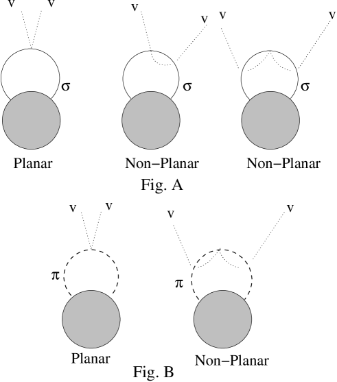
FIG. 18.: Fig. A gives the rule P:NP = 1:2 for $v^{2}$ insertions in $\sigma$ propagators and Fig. B gives the rule P:NP = 1:1 for $\pi$ propagators with $v^{2}$ insertions

Each $v^{2}$ insertion on the propagators would divide the diagram into Planar and Non-Planar parts as shown in Figures A and B. The ratio in which these insertions should divide the diagrams in order to preserve renormalizability of the theory has been worked out by remembering that the $v$ and the $\sigma$ lines originally correspond to $\phi_{1}$ lines in the unbroken theory and the $\pi$ to the $\phi_{2}$.

With this rule of dividing the UV divergent terms into Planar and Nonplanar parts, the Planar terms from equation (57) are,

$$\Gamma_{P}^{\sigma} = v_{0}\mu^{2}-v_{0}^{3}\lambda+v_{0}[-2\lambda(\Lambda^{2}+\mu^{2}ln(\frac{\Lambda^{2}}{m_{\sigma}^{2}})-v_{0}^{2}\lambda ln(\frac{\Lambda^{2}}{m_{\sigma}^{2}}))]+v_{0}[-\lambda(\Lambda^{2}+\mu^{2}ln(\frac{\Lambda^{2}}{m_{\pi}^{2}})-\frac{1}{2}v_{0}^{2}\lambda ln(\frac{\Lambda^{2}}{m_{\pi}^{2}}))]$$ (87)

$$= v_{0}\mu^{2}-v_{0}^{3}\lambda+v_{0}[-3\lambda\Lambda^{2}-3\lambda\mu^{2}ln(\frac{\Lambda^{2}}{m_{\sigma}^{2}})+\frac{5}{2}v_{0}^{2}\lambda^{2}ln(\frac{\Lambda^{2}}{m_{\sigma}^{2}}))+\frac{1}{2}\lambda^{2}v_{0}^{2}ln\frac{m_{\sigma}^{2}}{m_{\pi}^{2}}-\lambda\mu^{2}ln\frac{m_{\sigma}^{2}}{m_{\pi}^{2}}]$$ (88)

Apart from the tree-level and the UV divergent pieces, equation (59) contains the $ln(\frac{m_{\sigma}^{2}}{m_{\pi}^{2}})$ terms. While showing that the Ward Identity (11) holds, we would need to show that these terms also add up to the same for the $\sigma$ tadpole and the $\pi$-$\pi$ amplitudes. We shall not be verifying that the Ward Identity holds for all the nonplanar terms, but only for the coefficient of $ln(\frac{m_{\sigma}^{2}}{m_{\pi}^{2}})$ terms coming from these nonplanar terms. Note that the IR terms in equation (57) result from the Nonplanar terms when we finally set the external momentum on the $v$ legs to zero. These Nonplanar terms are of the form,

$$S_{NP(1)}^{\sigma}=\int dp_{1}dp_{2}[-\lambda(\Lambda_{eff}^{2}+\mu^{2}ln(\frac{\Lambda_{eff}^{2}}{m_{\sigma}^{2}})-3v_{0}^{2}\lambda ln(\frac{\Lambda_{eff}^{2}}{m_{\sigma}^{2}}))]\sigma(p_{1})v(p_{2})\delta(p_{1}+P_{2})$$ (89)

There are other contributions to the Nonplanar terms. These are from equation (57), when the $v_{0}^{2}$ terms are divided into P:NP. These are,

$$S_{NP(2)}^{\sigma}=\int dp_{1}dp_{2}[4v_{0}^{2}\lambda^{2}ln(\frac{\Lambda_{eff}^{2}}{m_{\sigma}^{2}})+\frac{1}{2}v_{0}^{2}\lambda^{2}ln(\frac{\Lambda_{eff}^{2}}{m_{\pi}^{2}})]\sigma(p_{1})v(p_{2})\delta(p_{1}+P_{2})$$ (90)

$$S_{NP}^{\sigma} = S_{NP(1)}^{\sigma}+S_{NP(2)}^{\sigma}$$ (91)

$$= \int dp_{1}dp_{2}[-\lambda\Lambda_{eff}^{2}-\lambda\mu^{2}ln(\frac{\Lambda_{eff}^{2}}{m_{\sigma}^{2}})+\frac{15}{2}v_{0}^{2}\lambda^{2}ln(\frac{\Lambda_{eff}^{2}}{m_{\sigma}^{2}})+\frac{1}{2}v_{0}^{2}\lambda^{2}ln(\frac{m_{\sigma}^{2}}{m_{\pi}^{2}})]\sigma(p_{1})v(p_{2})\delta(p_{1}+P_{2})$$ (92)

The other finite terms are the same as that of the broken phase of the commutative O(2) theory as explained earlier. Note that the external momenta dependences in the $\Lambda_{eff}^{2}$ in equations (60), (61) may be different. However we are only interested in the coefficient of the $ln(\frac{m_{\sigma}^{2}}{m_{\pi}^{2}})$ term which is shown in equation (63). Now, taking the contributions from both the planar and the nonplanar parts, the coefficient of $ln(\frac{m_{\sigma}^{2}}{m_{\pi}^{2}})$ in $\sigma$ tadpole amplitude is, $(\lambda^{2}v_{0}^{2}-\lambda\mu^{2})$.

We now proceed with the computation of the $\pi$-$\pi$ amplitude and show that this rule can be consistently used to show the renormalizability of this Broken Phase.

B $\pi$-$\pi$ Amplitude

FIG. 19.:

The terms that will contribute here are from equations (36), (38), (40), (44) and (48) and is shown diagramatically in Fig.19.

$$S_{eff}^{\pi\pi} = \int dp\frac{1}{2}\pi(p)[-p^{2}+\mu^{2}-\lambda v_{0}^{2}]\pi(-p)$$ (93)

$$+ \int dp_{1}dp_{2}\frac{1}{2}[-2\lambda(\Lambda^{2}-m_{\pi}^{2}ln(\frac{\Lambda^{2}}{m_{\pi}^{2}}))+NP+F]\pi(p_{1})\pi(p_{2})\delta(p_{1}+p_{2})$$ (94)

$$+ \int dp_{1}dp_{2}\frac{1}{2}[-\lambda(\Lambda^{2}-m_{\sigma}^{2}ln(\frac{\Lambda^{2}}{m_{\sigma}^{2}}))+NP+F]\pi(p_{1})\pi(p_{2})\delta(p_{1}+p_{2})$$ (95)

$$+ \int dp_{1}dp_{2}dp_{3}dp_{4}\frac{1}{4}f_{2}(p_{1},p_{2},p_{3},p_{4})[\lambda^{2}\int_{0}^{1}dxln(\frac{\Lambda^{2}}{\Delta^{2}})+NP+F]\pi(p_{1})\pi(p_{2})v(p_{3})v(p_{4})$$ (96)

$$\Gamma^{\pi\pi} = [-p^{2}+\mu^{2}-\lambda v_{0}^{2}]+[-2\lambda(\Lambda^{2}+\mu^{2}ln(\frac{\Lambda^{2}}{m_{\pi}^{2}})-\lambda v_{0}^{2}ln(\frac{\Lambda^{2}}{m_{\pi}^{2}}))+IR+F]$$ (97)

$$+ [-\lambda(\Lambda^{2}+\mu^{2}ln(\frac{\Lambda^{2}}{m_{\sigma}^{2}})-3\lambda v_{0}^{2}ln(\frac{\Lambda^{2}}{m_{\sigma}^{2}}))+IR+F]$$ (98)

$$+ [\frac{1}{2}\lambda^{2}v_{0}^{2}\int_{0}^{1}dxln(\frac{\Lambda^{2}}{\Delta^{2}})+IR+F]$$ (99)

The expressions under the integral over $x$ is the planar contribution from the last graph of Fig.19. If $p$ be the total momentum going in and out of the loop then,

$$-\Delta^{2}=p^{2}x(1-x)+x(m_{\sigma}^{2}-m_{\pi}^{2})-m_{\sigma}^{2}$$ (100)

After the division of the UV divergent terms into Planar and Nonplanar terms in appropriate ratios, we have,

$$\Gamma_{P}^{\pi\pi} = [-p^{2}+\mu^{2}-\lambda v_{0}^{2}]+[-2\lambda(\Lambda^{2}+\mu^{2}ln(\frac{\Lambda^{2}}{m_{\pi}^{2}})-\frac{1}{2}\lambda v_{0}^{2}ln(\frac{\Lambda^{2}}{m_{\pi}^{2}}))]$$ (101)

$$+ [-\lambda(\Lambda^{2}+\mu^{2}ln(\frac{\Lambda^{2}}{m_{\sigma}^{2}})-\lambda v_{0}^{2}ln(\frac{\Lambda^{2}}{m_{\sigma}^{2}}))]+[\frac{1}{2}\lambda^{2}v_{0}^{2}ln(\frac{\Lambda^{2}}{m_{\sigma}^{2}})]-[\frac{1}{2}\lambda^{2}v_{0}^{2}\int_{0}^{1}dxln(\frac{\Delta^{2}}{m_{\sigma}^{2}})]$$ (102)

$$\Gamma_{P}^{\pi\pi}\mid_{p=0} = [\mu^{2}-\lambda v_{0}^{2}]+[-3\lambda\Lambda^{2}-3\lambda\mu^{2}ln(\frac{\Lambda^{2}}{m_{\sigma}^{2}})+\frac{5}{2}\lambda^{2}v_{0}^{2}ln(\frac{\Lambda^{2}}{m_{\sigma}^{2}})+\lambda^{2}v_{0}^{2}ln(\frac{m_{\sigma}^{2}}{m_{\pi}^{2}})-2\lambda\mu^{2}ln(\frac{m_{\sigma}^{2}}{m_{\pi}^{2}})]-\frac{1}{4}[\lambda^{2}v_{0}^{2}-\lambda\mu^{2}]$$ (103)

The last term in the bracket in equation (68) is the contribution from the integral over $x$, the integration is performed in the limit $p\rightarrow 0$.

We now write down the Nonplanar terms including the contributions from equation (65) occuring from the division of $v_{0}^{2}$ terms in the UV divergent terms. Here again the purpose is to extract the coefficient of $ln(\frac{m_{\sigma}^{2}}{m_{\pi}^{2}})$ term, and although the various $\Lambda_{eff}^{2}$ may have different momenta dependences these terms are all IR divergent when $v$ is set to a constant and the external $\pi$ momentum is zero.

$$S_{NP(1)}^{\pi\pi} = \int dp_{1}dp_{2}[-\lambda(\Lambda_{eff}^{2}+\mu^{2}ln(\frac{\Lambda_{eff}^{2}}{m_{\pi}^{2}})-\lambda v_{0}^{2}ln(\frac{\Lambda_{eff}^{2}}{m_{\pi}^{2}}))+\frac{7}{2}\lambda^{2}v_{0}^{2}\int_{0}^{1}dxln(\frac{\Lambda_{eff}^{2}}{\Delta^{2}})]\pi(p_{1})\pi(p_{2})\delta(p_{1}+p_{2})$$ (104)

$$S_{NP(2)}^{\pi\pi} = \int dp_{1}dp_{2}[\lambda^{2}v_{0}^{2}ln(\frac{\Lambda_{eff}^{2}}{m_{\pi}^{2}})+2\lambda^{2}v_{0}^{2}ln(\frac{\Lambda_{eff}^{2}}{m_{\sigma}^{2}})]\pi(p_{1})\pi(p_{2})\delta(p_{1}+p_{2})$$ (105)

$$S_{NP}^{\pi\pi} = S_{NP(1)}^{\pi\pi}+S_{NP(2)}^{\pi\pi}$$ (106)

$$= \int dp_{1}dp_{2}[-\lambda\Lambda_{eff}^{2}-\lambda\mu^{2}ln(\frac{\Lambda_{eff}^{2}}{m_{\pi}^{2}})+\frac{15}{2}\lambda^{2}v_{0}^{2}ln(\frac{\Lambda_{eff}^{2}}{m_{\pi}^{2}})+2\lambda^{2}v_{0}^{2}ln(\frac{m_{\sigma}^{2}}{m_{\pi}^{2}})-\lambda\mu^{2}ln(\frac{m_{\sigma}^{2}}{m_{\pi}^{2}})$$ (107)

$$- \frac{7}{2}\lambda^{2}v_{0}^{2}\int_{0}^{1}dxln(\frac{\Delta^{2}}{m_{\sigma}^{2}})]\pi(p_{1})\pi(p_{2})\delta(p_{1}+p_{2})$$ (108)

The integral in $x$ can be done with $p\rightarrow 0$, when the nonplanar terms become IR divergent. The coefficient of the $ln(\frac{m_{\sigma}^{2}}{m_{\pi}^{2}})$ term from the nonplanar parts is, $[2\lambda^{2}v_{0}^{2}-\lambda\mu^{2}]-[\frac{7}{4}(\lambda^{2}v_{0}^{2}-\lambda\mu^{2})]$. Now adding the contributions from both the planar as well as the nonplanar parts the coefficient is,$(\lambda^{2}v_{0}^{2}-\lambda\mu^{2})$, which is exactly equal to what we had obtained for the $\sigma$ tadpole amplitude.

Comparing the UV divergences of $\Gamma_{P}^{\sigma}$ equation (59) and $\Gamma_{P}^{\pi\pi}$ equation (68), the quadratic and the lograthimic divergences are identical and thus can be cancelled by the counterterms. This shows that we have retained the renormalizability of the theory. Note that the weights of the nonplanar terms in equations (63) and (72) also match (although we have not verified equality of these terms with proper momenta dependences). Furthermore, since the action and the measure are O(2) invariant, as are the UV divergent pieces, we can conclude that the rest of the UV finite (including IR divergent) parts of $\Gamma$ satisfy the Ward identity. This would normally imply the masslessness of the pion. However we do not know whether the IR divergences imply that the symmetric vacuum has lower energy.

VI conclusion

We have shown that for the spontaneously broken noncommutative scalar field theory with global O(2) symmetry there is no violation of Ward Identity and the theory is renormalizable to one loop. The violations of Ward Identity as shown in [32] can be traced to the dropping of UV divergent surface terms. A modification of the prescription, where we treat the shift $v$ as nonconstant background field and restrict it to a constant only after all loop computations, allows us to keep track of all these surface terms. It is also necessary to keep track of the division of the terms into Planar and Non-Planar parts. In particular the mass insertions corresponding to the $v_{0}^{2}$ terms have to be divided into appropriate proportions to preserve the renormalizability of the broken theory.

The one loop Infrared divergences seem to provide an infinite positive $(mass)^{2}$ for all the fields of the theory. Thus for finite negative tree level $(mass)^{2}$ values, one would conclude that there is symmetry restoration at one loop. However until one has a way to make sense of the IR divergences this would be quite speculative. We think this is one of the outstanding issues in this area. Perhaps string theory can provide a clue to the resolution.

Acknowledgements :

We thank N. D. Haridass for useful discussions and careful reading of the manusctipt.

A Feynman Rules for the Symmetric phase

Propagators :

FIG. 20.:

$$\phi_{1}:\frac{1}{k^{2}-\mu^{2}}$$ (A1)

$$\phi_{2}:\frac{1}{k^{2}-\mu^{2}}$$ (A2)

Interaction Vertex :

FIG. 21.:

$$=-2\lambda[\delta^{ij}\delta^{kl}cos(\frac{p_{1}\wedge p_{2}}{2})cos(\frac{p_{3}\wedge p_{4}}{2})+\delta^{ik}\delta^{jl}cos(\frac{p_{1}\wedge p_{3}}{2})cos(\frac{p_{2}\wedge p_{4}}{2})$$ (A3)

$$+ \delta^{il}\delta^{jk}cos(\frac{p_{1}\wedge p_{4}}{2})cos(\frac{p_{2}\wedge p_{3}}{2})]$$ (A4)

where,

$$p_{i}\wedge p_{j}=p_{i\mu}\theta^{\mu\nu}p_{j\nu}$$ (A5)

Four Point Amplitude :

FIG. 22.:

$$=4\lambda^{2}\frac{1}{2}\int\frac{d^{4}k}{(2\pi)^{4}}\frac{V_{T}(p_{1},p_{2},p_{3},p_{4},p,k)}{(k^{2}-\mu^{2})[(p-k)^{2}-\mu^{2}]}$$ (A6)

Where,

$$V_{T}(p_{1},p_{2},p_{3},p_{4},p,k) = [2\delta^{ij}\delta^{kl}[cos^{2}(\frac{k\wedge p}{2})cos(\frac{p_{1}\wedge p_{2}}{2})cos(\frac{p_{3}\wedge p_{4}}{2})$$ (A7)

$$+ cos(\frac{p\wedge k}{2})cos(\frac{p_{1}\wedge p_{2}}{2})cos(\frac{p_{3}\wedge(p_{4}+k)}{2})cos(\frac{p_{4}\wedge k}{2})$$ (A8)

$$+ cos(\frac{p\wedge k}{2})cos(\frac{p_{1}\wedge p_{2}}{2})cos(\frac{p_{4}\wedge(p_{3}+k)}{2})cos(\frac{p_{3}\wedge k}{2})$$ (A9)

$$+ cos(\frac{p\wedge k}{2})cos(\frac{p_{3}\wedge p_{4}}{2})cos(\frac{p_{2}\wedge(p_{1}-k)}{2})cos(\frac{p_{1}\wedge k}{2})$$ (A10)

$$+ cos(\frac{p\wedge k}{2})cos(\frac{p_{3}\wedge p_{4}}{2})cos(\frac{p_{1}\wedge(p_{2}-k)}{2})cos(\frac{p_{2}\wedge k}{2})]$$ (A11)

$$+ \delta^{il}\delta^{jk}[cos(\frac{p_{1}\wedge k}{2})cos(\frac{p_{4}\wedge k}{2})cos(\frac{p_{2}\wedge(p_{1}-k)}{2})cos(\frac{p_{3}\wedge(p_{4}+k)}{2})$$ (A12)

$$+ cos(\frac{p_{2}\wedge k}{2})cos(\frac{p_{3}\wedge k}{2})cos(\frac{p_{1}\wedge(p_{2}-k)}{2})cos(\frac{p_{4}\wedge(p_{3}+k)}{2})]$$ (A13)

$$+ \delta^{ik}\delta^{jl}[cos(\frac{p_{1}\wedge k}{2})cos(\frac{p_{3}\wedge k}{2})cos(\frac{p_{2}\wedge(p_{1}-k)}{2})cos(\frac{p_{4}\wedge(p_{3}+k)}{2})$$ (A14)

$$+ cos(\frac{p_{2}\wedge k}{2})cos(\frac{p_{4}\wedge k}{2})cos(\frac{p_{1}\wedge(p_{2}-k)}{2})cos(\frac{p_{3}\wedge(p_{4}+k)}{2})]$$ (A15)

$$p_{1}+p_{2}=p=-(p_{3}+p_{4})$$ (A17)

The other two channels (s and u) can be obtained by interchanging j and k and j and l and the appropriate momenta.

REFERENCES

• [1] A. Connes, J. Lott, Nucl.Phys.Proc.Suppl. 18B (1991) 29-47 A. Connes, M. R. Douglas, and A. Schwarz, hep-th/9711162, JHEP 02 (1998) 003
• [2] A. P. Balachandran, G. Bimonte, E. Ercolessi, G. Landi, F. Lizzi, G. Sparano and P. Teotonio-Sobrinho, hep-th/9403067, Nucl.Phys.Proc.Suppl. 37c (1995)
• [3] N. Seiberg and E. Witten, hep-th/9908142 JHEP 09 (1999) 032
• [4] T. Filk, Phys. Lett. B376 (1996)
• [5] S. Minwalla, M.V. Raamsdonk and N. Seiberg, hep-th/9912072 JHEP 02 (2000) 020
• [6] M.V. Raamsdonk and N. Seiberg, hep-th/0002186 JHEP 03 (2000) 035
• [7] J. C. Virally and J. M. Gracia-Bondia, hep-th/9804001 Int. J. Mod. Phys. A14 (1999) 1305
• [8] M. Chaichian, A. Demichev and P. Presnajder, hep-th/9812180, hep-th/9904132
• [9] M. Sheikh-Jabbari, hep-th/9903107, JHEP 06 (1999) 015
• [10] A. P. Balachandran, T. R. Govindarajan, B. Ydri, hep-th/9911087 Mod. Phys. Lett. A15 (2000) 1279
• [11] C. P. Martin and D. Sanchez-Ruiz, hep-th/9903007, Phys.Rev.Lett. 83 (1999)
• [12] I. Chepelev and R. Roiban, hep-th/9911098,JHEP 05 (2000) 037
• [13] W. H. Huang, hep-th/0009067 Phys.Lett. B496 (2000)
• [14] I. A. Aref’eva, D. M. Belov and A. S. Koshelev,hep-th/9912075,Phys. Lett. B476 (2000) 431; hep-th/0001215 I. Ya. Aref’eva, D. M. Belov, A. S. Koshelev and O. A. Rytchkov hep-th/0003176
• [15] S. S. Gubser and S. L. Sondhi, hep-th/0006119
• [16] A. Micu, M.M. Sheikh-Jabbari, hep-th/0008057
• [17] N. Seiberg, L. Susskind, N. Toumbas, hep-th/0005015, JHEP 06 (2000) 044
• [18] J. Gomis and T. Mehen, hep-th/0005129, Nucl.Phys. B591 265 (2000)
• [19] R. Gopakumar, S. Minwalla, and A. Strominger, hep-th/0003160, JHEP 05 (2000) 020
• [20] Alec Matusis, Leonard Susskind, Nicolaos Toumbas, hep-th/0002075
• [21] S. Iso, H. Kawai and Y. Kitazawa, hep-th/0001027, Nucl.Phys. B576 (2000)
• [22] T. Krajewski and R. Wulkenhaar, hep-th/9903187, Int.J.Mod.Phys A15 (2000)
• [23] M. Haykawa, hep-th/9912167
• [24] C. P. Martin and D. Sanchez-Ruiz, hep-th/0012024, Nucl.Phys. B598 (2000) 348-370
• [25] M. M. Sheikh-Jabbari, hep-th/0001167, Phys.Rev.Lett.84 (2000) 5265
• [26] M. Chaichan, A. Demichev, P. Presnajder, M. M. Sheikh-Jabbari and A. Tureanu, hep-th/0012175
• [27] A. Matusis, L. Susskind and N. Toumbas, hep-th/0002075, JHEP 0012 (2000) 002
• [28] F. Ardalan and N. Sadoogi, hep-th/0002143
• [29] I. F. Raib and M. M. Sheikh-Jabbari, hep-th/0008132, JHEP 08 (2000) 045
• [30] N. Chair and M. M. Sheikh-Jabbari, hep-th/0009037
• [31] F. Ruiz-Ruiz, hep-th/0012171, Phys.Lett. B502 (2001) 274-278
• [32] B. A. Campbell and K. Kaminsky, hep-th/0003137 Nucl. Phys B581 240 (2000), hep-th/0102022
• [33] Frank J. Petriello, hep-th/0101109
• [34] Emil T. Akhmedov, Philip DeBoer and Gordon W. Semenoff, hep-th/0010003, hep-th/0103199
• [35] M. Peskin and D. Schroeder, An Introduction to Quantum Field Theory, Perseus Books, (1995)
• [36] S. Coleman,Commun.Math.Phys.31 259-264,(1973)