Pyrotechnic Universe

Abstract

One of the central points of the ekpyrotic cosmological scenario based on Hor̆ava-Witten theory is that we live on a negative tension brane. However, the tension of the visible brane is positive in the usual HW phenomenology with stronger coupling on the hidden brane, both for standard and non-standard embedding. To make ekpyrotic scenario realistic one must solve the problem of the negative cosmological constant on the visible brane and fine-tune the bulk brane potential with an accuracy of $10^{-50}$. In terms of a canonically normalized scalar field $\phi$ describing the position of the brane, this potential must take a very unusual form ${\cal V}(\phi)=-10^{-22}M_{p}^{4}\exp\left(-{5000\,\phi\over M_{p}}\right)$. We describe the problems which appear when one attempts to obtain this potential in string theory. The mechanism for the generation of density perturbations in this scenario is not brane-specific; it is a particular limiting case of the mechanism of tachyonic preheating. Unlike inflation, this mechanism exponentially amplifies not only quantum fluctuations, but also initial inhomogeneities. As a result, to solve the homogeneity problem in this scenario, one would need the branes to be parallel to each other with an accuracy better than $10^{-60}$ on a scale $10^{30}$ times greater than the distance between the branes. Thus, at present, inflation remains the only robust mechanism that produces density perturbations with a flat spectrum and simultaneously solves all major cosmological problems.

I Introduction

After 15 years of development of string theory and M-theory we are still faced with the challenging problem of constructing a consistent and realistic stringy cosmology. An interesting step in this direction has recently been made by Khoury, Ovrut, Steinhardt and Turok, who suggested a three-brane cosmological model based on the Hor̆ava-Witten theory, and argued that it may resolve all major cosmological problems without any use of inflation [1]. Their model was called the ekpyrotic universe, from the Greek-derived word ekpyrosis.

The basic idea of this scenario is that initially the universe was in a nearly BPS state consisting of two parallel branes, and that we live on the brane with negative tension. Then the brane with positive tension splits into two positive tension branes, one of which (bulk brane) starts moving towards our brane. The big bang corresponds to the moment when the bulk brane hits our brane; the collision makes the universe hot. It was argued that the flatness of the branes in the nearly BPS state solves the homogeneity and flatness problems, whereas quantum fluctuations of the bulk brane result in the large-scale density perturbations on our brane when these branes collide. In this paper we re-examine some of the basic premises of this model. We will try to verify whether it follows from string theory and whether it indeed can solve all major cosmological problems without the help of inflation. In this sense, our paper will be devoted to an epicrisis of ekpyrosis.

One of the central points of the ekpyrotic scenario is that we live on a negative tension brane, and the warp factor (the volume of the Calabi-Yau space) decreases towards the visible brane. In the original version of Ref. [1] one can read: As we will see in Section VB, it will be necessary for the visible brane to be in the small-volume region of space-time. The authors repeatedly emphasized that this condition is very important for their scenario and argued that it results in a distinguishing feature of their model: a blue spectrum of density perturbations.

However, as we will explain in Section III, the standard HW phenomenology [3, 4, 5] (both for standard and non-standard embedding) is based on the assumption that the tension of the visible brane is positive, and the warp factor increases towards the visible brane. There were two main reasons for such an assumption. First of all, in practically all known versions of the HW phenomenology, with few exceptions, a smaller group of symmetry (such as $E_{6}$) lives on the positive tension brane and provides the basis for GUTs, whereas the symmetry $E_{8}$ on the negative tension brane may remain unbroken. It is very difficult to find models where $E_{6}$ or $SU(5)$ live on the negative tension brane [6, 7].

There is another reason why the tension of the visible brane is positive in the standard HW phenomenology [3, 4, 5]: The square of the gauge coupling constant is inversely proportional to the Calabi-Yau volume [3]. On the negative tension brane this volume is greater than on the positive tension one, see e.g. [1]. In the standard HW phenomenology it is usually assumed that we live on the positive tension brane with small gauge coupling, ${g^{2}_{GUT}\over 4\pi}\sim 0.04$. On the hidden brane with negative tension the gauge coupling constant becomes large, ${g^{2}_{hidden}\over 4\pi}=O(1)$, which makes the gaugino condensation possible [3, 4, 5]. It is not impossible to have a consistent phenomenology with the small gauge coupling on the hidden brane, but this is an unconventional and not well explored possibility [6].

Thus, we believe that the ekpyrotic scenario is at odds with the standard HW phenomenology as defined in [3, 4, 5]. The relevant issue is not the standard versus non-standard embedding, but Hor̆ava-Witten phenomenology [3, 4, 5] versus Benakli-Lalak-Pokorski-Thomas [6] phenomenology. As explained in Section VB of [1], the reason to assume that the CY volume should decrease towards the visible brane was rooted in the idea that this is required for generation of density perturbations in the ekpyrotic scenario. However, as we will show in Section IV, this requirement is not necessary.

To improve the ekpyrotic scenario one would need to change the sign of the brane tension. In this case the warp factor decreases towards the hidden brane. This changes the shape of the spectrum of density perturbations from blue to red. However, one cannot simply flip the sign of the tension in the model leaving all other parameters intact because it would introduce a singularity between the branes. One needs to change other parameters of the model as well. We will call the improved scenario pyrotechnic to emphasize its relation to the ekpyrotic scenario, but also to indicate that it remains vulnerable to other problems to be discussed below. In this scenario, unlike in the ekpyrotic scenario, we will not make any attempts to avoid inflation.

The critical assumption of the ekpyrotic scenario discussed in Section V is that the bulk brane interacts with the visible brane with the negative potential

$$V(Y)=-ve^{-|\alpha|mY}\ .$$ (1)

However, in cases where this potential has been explicitly calculated, it was shown to be positive [13]. Moreover, in general the potential contains two terms, $e^{-|\alpha|mY}$ and $e^{-|\alpha|m(R-Y)}$, to include bulk brane interactions with hidden and visible branes. Originally, potentials of such type were supposed to describe interactions of the visible brane or the bulk brane with the hidden brane with unbroken $E_{8}$ [14]. In such a case the potential would be $V(Y)\sim-ve^{-|\alpha|m(R-Y)}$, where $R-Y$ is the distance between the bulk brane and the hidden brane. In the ekpyrotic scenario all terms like that should be forbidden, which may be difficult to achieve unless one assumes that originally our brane was the end-of-the-world $E_{8}$ brane, and it became the physical brane after the brane collision. No theoretical description of such a process is presently available; all previous attempts to do so assumed that $E_{8}$ is already broken and colliding branes have comparable tensions, which is not the case in [1].

The peculiar nature of the brane potential $V(Y)\sim-ve^{-|\alpha|mY}$ becomes manifest if one writes it in terms of a canonically normalized scalar field $\phi$ describing the position of the brane: ${\cal V}(\phi)=-10^{-22}M_{p}^{4}\exp\left(-{5000\,\phi\over M_{p}}\right)$ for the specific choice of the parameters $v$, $\alpha$, $m$ requested by [1]. While potentials $\sim\exp{c\phi\over M_{p}}$ with $c=O(1)$ often appear in string theory, such terms as $\exp\left(-{5000\,\phi\over M_{p}}\right)$ are rather unprecedented.

At the first glance, the theory of the generation of density perturbations in the ekpyrotic scenario seems very complex and brane-specific, as indicated by the statement of [1] that this mechanism requires the warp factor to decrease towards the visible brane. However, in Section IV we show that the theory of the generation of density perturbations used in [1] is in fact a limiting case of the theory of tachyonic preheating recently developed in [10]. The theory of this effect is very simple. It works for branes in 5d as well as for the usual scalar field in 4d due to the exponential growth of long wavelength fluctuations in theories with concave effective potentials ($V^{\prime\prime}<0$). The spectrum of perturbations may be flat, but it may also be red or blue, depending on the choice of the potential. Power-law potentials typically are unacceptable. One should make the very special choice of a nearly exponential potential to produce a cosmologically acceptable spectrum. To make this mechanism realistic, one must solve the problem of the negative cosmological constant on the visible brane and fine-tune the value of the bulk brane potential with an accuracy of $10^{-50}$. If one does not perform this fine-tuning, the standard inflationary mechanism for the generation of density perturbations turns on, and the model becomes very similar to the model of brane inflation proposed by Dvali and Tye [11].

If one resolves all of these problems, and the tachyonic mechanism for the generation of density perturbations begins to work, then we will have a new problem, which may be much more serious than the previous ones: tachyonic instability exponentially amplifies not only quantum fluctuations but also initial inhomogeneities. As a result, to solve the homogeneity problem in this scenario one would need the branes to be parallel to each other with an accuracy better than $10^{-60}$ on a scale $10^{30}$ times greater than the distance between the branes, see Section VI. Since the initial state is not really a true BPS state but rather some unstable and evolving configuration, we do not see any reason why our universe must be so incredibly homogeneous from the very beginning.

Thus we believe that at present inflation remains the only robust mechanism that produces density perturbations with a flat spectrum and simultaneously solves all major cosmological problems.

II General setup for ekpyrotic universe

The ekpyrotic scenario consists of many parts related to the M-theory and cosmology. M-theory issues, including the sign of the tensions of the visible and hidden brane and the BPS nature of the 3 brane solution, will be discussed in Sec. 3. For a cosmologist, the end result of the story from M-theory as presented in [1] is the following:

There is a static three brane solution for the space-time metric and the dilaton $e^{\phi}$ (volume of the Calabi-Yau space) given by

$$ds^{2}=D(y)(-N^{2}d\tau^{2}+A^{2}d\vec{x}^{2})+B^{2}D^{4}(y)dy^{2}\ ,$$ (2)

$$e^{\phi}=BD^{3}(y)\ ,$$ (3)

$$D(y)=\alpha y+C\;\;\;\;\;\;\;\;\;\;\;\;\;\;\;\;\;\;\;\;\;\;\;\;\;\;{\rm for}\;\;y<Y$$ (4)

$$\;\;\;\;\;\;\;\;\;=(\alpha-\beta)y+C+\beta Y\;\;\;\;\;\;\;{\rm for}\;\;y>Y,$$ (5)

where $A,B,C,N$ are constants and $C>0$. The boundary branes are located at $y=0$ and $y=R$, and the bulk brane is located at $y=Y$, where $0\leq Y\leq R$. The tension of the visible brane at $y=0$ is $-\alpha$ and is negative. The tension of the bulk brane $\beta$ is positive and the tension of the hidden brane at $y=R$ is positive and equals $\alpha-\beta$. One assumes that $\beta\ll\alpha$, so the bulk brane is relatively light. The visible brane at $y=0$ lies in the region of smaller volume while $y=R$ lies in the region of larger volume. Indeed, $D(0)=C$ and $D(R)=C+\alpha R$ and $\alpha$ is positive, so $D(0)<D(R)$. This property is considered one of the most important features of the scenario.

The light bulk brane may either appear spontaneously from the hidden brane or it may also exist from the very beginning, i.e. one starts with two boundary branes and one bulk brane. The three brane configuration is assumed to be in a nearly BPS state. It is argued that the universe must be homogeneous because the BPS brane configuration is homogeneous. The bulk brane has a kinetic term and a potential, which for a “successful example” is chosen to be $V(Y)=-ve^{-m\alpha Y}$. Additionally it is assumed that at small $Y$ the potential suddenly becomes zero due to some nonperturbative effects.

Due to the slight contraction of the scale factor on the bulk brane, the bulk brane carries some residual kinetic energy immediately before the collision with the visible brane. After the collision, this residual kinetic energy transforms into radiation which will be deposited in the three dimensional space of the visible brane. The visible brane, now filled with hot radiation, somehow begins to expand as a flat FRW universe. However, the temperature is not high enough to trigger phase transitions in GUTs and produce primordial monopoles. Quantum fluctuations of the position of the bulk brane generated during its motion from $Y=R$ to $Y=0$ will result in density fluctuations with a nearly flat spectrum. The spectrum will have a slightly blue tilt for the exponential potential $V(Y)$.

The set of parameters used in [1] is $\alpha=250M_{5}$, $\beta=0.1M_{5}$, $B=10^{-3}$, $C=100$, $R=M_{5}^{-1}$, $v\sim 10^{-10}$, $m=1$, and $M_{5}=10^{-2}M_{pl}$. A sketch of the model is given in Fig. 1.

The total setup is rather complicated, but the final picture allows for a dramatic simplification. Indeed, let us look first at the behavior of the factor $D(Y)$, which determines the metric in (5), during the whole process of motion of the bulk brane towards the visible brane. The motion begins at $Y=R=M_{5}^{-1}$ and ends at $Y=0$. During this process $D(Y)$ changes from $350$ to $100$, which is not that much. A more complicated analysis performed in [1] shows that the scale factors on all branes also do not change much. This suggests that the expansion of the universe and other complicated gravitational effects cannot be of any relevance to the possibility to solve major cosmological problems and to the basic mechanism of the generation of density perturbations. On the other hand, the authors of Ref. [1] emphasized that the decrease of $D(Y)$ towards the brane is crucially important and used the notion of the effective scale factor $a_{\rm{eff}}$ to explain the mechanism of production of density perturbations.

In this paper we will attempt to analyse this situation, starting from the M-theory part, and ending with a discussion of the cosmological density perturbations and homogeneity problem.

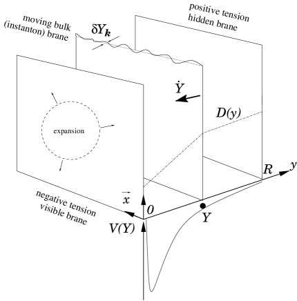
FIG. 1.: Sketch of the ekpyrotic scenario. We live on a brane with negative energy density. The Big Bang occurs when the bulk brane hits our brane. The bulk brane has potential energy $V(Y)$ which is postulated to have a very specific form: it is negative everywhere except on our brane, and its absolute value decreases exponentially at large $Y$. An important feature of this scenario is that the volume of space, controlled by the metric $D(Y)$, decreases near our brane, which makes the spectrum of perturbations blue.

III Supersymmetry and hidden-visible branes

A The action and the static solution

Here we consider the specific construction of [1] which starts with the solution of two boundary branes with almost opposite tensions and a bulk brane in between. We will explain the reason why the status of unbroken supersymmetry (BPS property) of this solution is problematic.

An effective five-dimensional action of heterotic M-theory is given in [1] the form:

$$S=\frac{M_{5}^{3}}{2}\int_{{\cal M}_{5}}d^{5}x\sqrt{-g}\left(R-\frac{1}{2}(\partial\phi)^{2}-\frac{e^{2\phi}{\cal F}^{2}}{5!}\right)$$ (6)

$$-3\sum_{i=1}^{3}\alpha_{i}M_{5}^{3}\int_{{\cal M}_{4}^{(i)}}d^{4}\xi_{(i)}\Bigl{(}\sqrt{-h_{(i)}}e^{-\phi}-\frac{\epsilon^{\mu\nu\kappa\lambda}}{4!}{\cal A}_{\gamma\delta\epsilon\zeta}\partial_{\mu}X^{\gamma}_{(i)}\partial_{\nu}X^{\delta}_{(i)}\partial_{\kappa}X^{\epsilon}_{(i)}\partial_{\lambda}X^{\zeta}_{(i)}\Bigr{)}\ .$$ (7)

Here $\phi$ the is the modulus of the Calabi-Yau (CY) threefold and ${\cal A}_{\gamma\delta\epsilon\zeta}$ is a 4-form gauge field. According to [1], the left brane is the visible one and it is assigned a negative tension $-\alpha=\alpha_{3}$, the bulk brane has positive tension $\beta=\alpha_{2}$ and the hidden brane has a positive tension $\alpha-\beta=\alpha_{1}$. The solution for the 5-form was written as follows:

$${\cal F}_{0123y}=\alpha D^{-2}\quad{\rm for}\qquad y<Y\,;\qquad{\cal F}_{0123y}=(\alpha-\beta)D^{-2}\quad{\rm for}\qquad y>Y$$ (8)

This action with three branes was not derived from supersymmetric theory. The action with two branes, which was derived in [5, 15, 16] from Hor̆ava-Witten (HW) theory, does not have a 4-form ${\cal A}_{\gamma\delta\epsilon\zeta}$, either in the bulk or on the branes. The appearance and the role of the 4-form gauge field in the five-dimensional supersymmetric bulk & brane action was explained in [17], but not in the context of HW theory. Recently it was shown in [18] that one can actually derive the action of the type of (7), but the factor in the action in front of ${\cal F}^{2}$ has to be corrected so that the action correspond to a bosonic part of the supersymmetric action. Also the factor and the sign in (8) have to be changed. It is easy to verify that the WZ term in the brane action does not cancel the BI term for the ‘solution’ given in [1], which proves that it is not a BPS solution before the correction is made. Thus one can find a BPS solution with the boundary and bulk brane present, see [18], but it is somewhat different from the one presented in [1].

Note that the BPS property of the classical solution is not the same as the requirement of unbroken supersymmetry. If the unbroken supersymmetry is established, the solution always has a BPS feature: the energy takes its minimal value and the supersymmetry bound is saturated, see e.g. [19]. However, non-supersymmetric BPS configurations are also possible. The difference is that for supersymmetric solutions one may expect that they will remain BPS states even with an account taken of quantum corrections, because of non-renormalization theorems for supersymmetric BPS states [20]. Meanwhile, non-supersymmetric BPS solutions may loose their BPS properties when quantum corrections are taken into account.

The issue of the unbroken supersymmetry for multi-domain wall solutions is more complicated than for other multi-brane solutions with co-dimension greater than 2, like multi-black-holes, multi-3-branes etc. The major difference is the behavior of the form fields at large distances. The supersymmetric domain walls are charged and the form fields are constant. They exist therefore only in the compact space with the vanishing total charge. The explicitly supersymmetric solution requires apart from supergravity the presence of the supersymmetric source actions which take care of the jump conditions on the wall.

The status of unbroken supersymmetry of the solution with two boundary branes without a bulk brane may be inferred from an action in [15] and [16] where the Born-Infeld part of the brane actions at the fixed points of the orbifold was given. However when the bulk brane is present in addition to boundary branes, the issue of unbroken supersymmetry is less clear. The supersymmetric bulk & brane construction of [17] (and HW theory) allows one to prove clearly the unbroken supersymmetry only for the case that the positive and negative tension branes are placed at the fixed points $0$ and $R$ of the orbifold ${S^{1}\over{\bf Z}_{2}}$. When the brane is not at the fixed points, the supersymmetry variation of the 4-form field in the Wess-Zumino term of the brane source action is not compensated by the supersymmetry variation of the Born-Infeld term. This makes the unbroken supersymmetry of the multi-domain walls problematic despite the fact that the bosonic solution with the jump of the 5-form field strength can be given.

Analogous problem exists for the multi-domain walls in D8-O8-system of type IIA string theory [21]. The variation of the R-R 9-form in the Wess-Zumino terms of the brane action depends on the NS-NS 2-form $B_{\mu\nu}$, whereas the supersymmetry variation of the Born-Infeld term does not depend on $B_{\mu\nu}$. Therefore the BI+WZ source action at the fixed points of the orientifolds is supersymmetric due to the fact that the NS-NS 2-form $B_{\mu\nu}$ is odd under ${\bf Z}_{2}$-symmetry and vanishes at the fixed points, but not between them. Therefore only when all D8 domain walls are coincident with orientifold planes, the supersymmetric bulk&brane action is available and the unbroken supersymmetry of the solution can be proven in [21]. The situation with the supersymmetry of the multi-wall solutions remains an open issue.

B Tension on visible brane

Let us now compare the ekpyrotic construction with HW theory. At the time when HW theory was suggested the issue of brane tension was not emphasized. More recently in the Randall-Sundrum I scenario [22] the positive and negative tension branes were given the names, ‘hidden’ and ‘visible’ brane, respectively. In this version the hidden brane was at the left, at $y=0$, and the visible brane at the right, at $y=\pi r_{c}$. The ‘visible’ brane, called sometimes the “TeV brane”, was designed to provide a solution of the hierarchy problem due to the fact that the warp factor decreases exponentially towards the ‘visible’ brane. In RS II [23] a dramatic change of the setup was made as the labels of ‘hidden’ and ‘visible’ branes were reversed. The former ’visible’ became hidden, the former ‘hidden’ became visible and it was suggested to send the negative tension hidden brane out of the world.

With all this in mind we will consider the known facts about HW and heterotic M-theory and the tensions of various branes in agreement with supersymmetry.

1 Standard embedding

In case of boundary branes of the original HW theory a standard embedding corresponds to a positive tension visible brane and negative tension hidden brane. Let us shortly remind how this happens. We will look at the heterotic M-theory in [16] where the Born-Infeld part of the brane actions were derived from HW theory. The tension of the visible brane is given by $-\alpha_{vis}$, where (we ignore here some irrelevant positive constants)

$$-\alpha_{vis}={1\over 8\pi^{2}}\int_{C}trR\wedge R=n\ ,$$

see for example eq. (3.13) in [16]. Here the integration is over a supersymmetric cycle of the CY manifold, and $R$ is the curvature form of the internal manifold. The integer $n$ characterizes the first Pontrjagin class of CY. Thus the tension of the visible brane is positive.

Let us present here a few important steps of the derivation of the tension formula. The tension on each brane, according to [16], is proportional to $-\alpha_{vis}={1\over 4\pi^{2}}\int_{C}(trF^{vis}\wedge F^{vis}-{1\over 2}trR\wedge R)\ ,$ and $-\alpha_{hid}={1\over 4\pi^{2}}\int_{C}(trF^{hid}\wedge F^{hid}-{1\over 2}trR\wedge R)$.

So far the visible and hidden brane are treated on an equal footing. The difference is in spin embedding in which only the visible brane participates. On the visible brane a standard spin connection embedding was performed so that the background is $trF^{vis}\wedge F^{vis}=trR\wedge R,\,F^{hid}=0,$ which implies that $tr(F^{vis}\wedge F^{vis}+F^{hid}\wedge F^{hid})-trR\wedge R=0\ .$. The $E_{8}$ gauge theory on the visible brane was broken to its subgroup $SU(3)\times E_{6}$ and after spin embedding on the visible brane there are $E_{6}$ gauge field excitations and on the hidden brane there are $E_{8}$ gauge field excitations. On the visible brane, where spin embedding takes place and $trF^{vis}\wedge F^{vis}=trR\wedge R$, we have

$$-\alpha_{vis}={1\over 8\pi^{2}}\int_{C}trR\wedge R>0\ ,$$ (9)

on the hidden one with $F^{hid}=0$ the tension is

$$-\alpha_{hid}=-{1\over 8\pi^{2}}\int_{C}trR\wedge R<0\ .$$ (10)

This explains how the visible brane in the original HW theory with standard embedding acquires a positive tension.

In [3] it was explained by Witten that the volume of the CY space $e^{\phi}=V$ at the visible brane at $y=0$ is larger than that at the hidden brane at $y=R$: $V(0)>V(R)$ and the gauge coupling on the hidden brane is stronger than the one on the visible brane, $g^{2}_{v}<g^{2}_{h}$ due to the inverse relation between the CY volume and the gauge coupling:

$${g^{2}_{v}\over g^{2}_{h}}\sim{V_{h}\over V_{v}}\sim{D^{3}(R)\over D^{3}(0)}\ .$$ (11)

The subsequent work on HW phenomenology [4] is based on a strong coupling at the hidden brane required for gaugino condensation on the hidden brane.

2 Non-standard embedding

The presence of the bulk brane requires using the non-standard embedding. The total tension (and the total charge) of all branes must vanish. In HW case the tension of the visible brane was positive and opposite to the tension of the hidden brane: $\alpha_{v}=-\alpha_{h}>0$. Now the new relation between brane tensions is

$$\alpha_{v}+\alpha_{h}+\beta=0\ .$$ (12)

This correspond to a cohomology constraint

$$c_{2}(V_{1})+c_{2}(V_{2})-c_{2}(TX)+[W]=0\ ,$$ (13)

where $[W]$ is the cohomology class associated with the five-branes and $c_{2}(V_{1}),c_{2}(V_{2}),c_{2}(TX)$ are the second Chern class of the gauge bundles $V_{1},V_{2}$ and of the tangent bundle $TX$, respectively.

The situation with the tension in non-standard embedding is the following. If one adds the bulk brane as a small modification of the previous two-brane configuration, one still has the visible brane with positive tension. However, in general one can have examples of both positive and negative tension on visible brane [6, 7].

In the ekpyrotic scenario the ratio between the tensions of boundary and bulk branes was chosen to be extremely small, ${\beta\over\alpha}=4\cdot 10^{-4}$. No examples with negative tension visible brane and ${\beta\over\alpha}\ll 1$ have been considered in the literature until very recently [7]. The examples considered in [7] require a special assumption that the volume of the base curves is much larger than the volume of the fiber curve in CY space. But even for such examples one still has an additional problem, which we are going to explain now.

The switch to the non-standard embedding does not change the relation between the volume of the Calabi-Yau space and the gauge coupling, Eq. (11). When the visible brane tension is positive (the warp factor decreases towards the negative tension brane), the standard HW phenomenology applies. One can have small gauge coupling ${g^{2}_{GUT}\over 4\pi}\sim 0.04$ on the visible brane, and large coupling ${g^{2}_{hidden}\over 4\pi}=O(1)$ on the hidden brane, which may lead to gaugino condensation [3, 4, 5].

However, when the visible brane tension is negative, a substantial modification of the standard HW phenomenology is required since in this case the gauge coupling constant on the hidden brane is smaller than on the visible brane. For example, with the parameters of [1] one has ${g^{2}_{hidden}\over 4\pi}\sim 10^{-3}$ on the hidden brane, which is way too small for the gaugino condensation. In general, one may try to develop acceptable phenomenology with stronger coupling observable sector [6], but this unconventional possibility is much less understood and developed that the standard HW phenomenology [3, 4, 5].

3 Tensions and BPS harmonic functions

The relation between brane tensions and the volume of CY manifold (inverse to the square of the gauge coupling) can be seen in the BPS solution where the sign of the tension on the visible brane defines the slope of the CY volume. The volume of the CY space is given by a harmonic function

$$e^{\phi}=BD^{3}\ ,\qquad D=C+\alpha y,\qquad y<Y\ ,$$ (14)

in notation of [1]. In [16], where the standard embedding was used, $C>0$, but the sign of $\alpha$ was not discussed. If it were noticed in [16] that $\alpha$ in this equation is negative one would be forced to rewrite the harmonic function as follows:

$$\tilde{D}=C-|\alpha|y\ ,\qquad\alpha<0\ ,$$ (15)

and comment on the existence of the critical distance between walls

$$\tilde{D}(y_{crit})=0\qquad\Rightarrow\qquad y_{crit}={C\over|\alpha|}\ .$$ (16)

This would prompt a requirement that the second wall has to cut off the singularity of the space time-metric when $\tilde{D}=0$ and therefore

$$R<y_{crit}\ .$$ (17)

Precisely this situation occurs in many cases of supersymmetric domain walls in [17, 21] where always the warp factor falls down away from the visible positive tension brane and one has to take care of the maximal distance between the walls.

However it was not noticed that the tension of the visible brane is positive in [16], where the standard embedding was used and the harmonic function was taken in the form $D=C+\alpha y$ instead of $\tilde{D}=C-|\alpha|y$. The authors of [1] used the same notation as in [16] and assumed, as equation $D=C+\alpha y$ suggests, that $\alpha$ is positive, i.e. the brane tension is negative, and $D(y)$ decreases near the visible brane at $y=0$. This assumption, combined with the idea that the density perturbations are produced in their scenario because of the decrease of $D(y)$ at small $y$, has led to the conclusion that it is “necessary for the visible brane to be in the small-volume region of space-time” [1].

However, as we will show in Sect. IV, this requirement is not necessary. We do not see any obvious reason to use unconventional versions of the HW theory and insist that we must live on the negative tension brane.

On the other hand, one cannot improve the situation by flipping the sign of $\alpha$ in all expressions in [1]. Indeed, according to the original version of the ekpyrotic scenario, $C=100$, and $\alpha=250M_{5}$. If we simply change the sign of $\alpha$ and take $\alpha=-250M_{5}$ we will find that the singularity of the metric appears between the walls at $y=0$ and at $y=R=M_{5}^{-1}$:

$$\tilde{D}=C-|\alpha|y=100-250M_{5}y\ ,$$ (18)

$$y_{crit}={2\over 5}M_{5}^{-1}<R=M_{5}^{-1}\ .$$ (19)

A quick fix of this problem is possible: one can change the parameters, e.g. by making $C$ larger or $|\alpha|$ smaller so that $y_{crit}={C\over|\alpha|}>R$ and the naked singularity at $y_{crit}$ is cut off by the hidden wall.

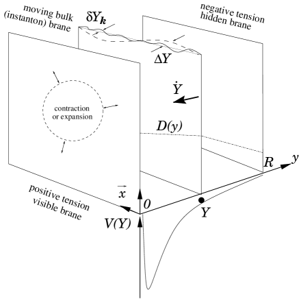
FIG. 2.: Sketch of the pyrotechnic scenario. We live on a brane with positive energy density. The volume of space controlled by the metric $D(Y)$ decreases near our brane, which gives a red tilt to the spectrum of perturbations. The mechanism for the generation of fluctuations $\delta Y_{k}$ in this scenario, as well as in the ekpyrotic scenario, amplifies all inhomogeneities, including classical inhomogeneities $\Delta Y$ of the bulk brane.

In what follows we will call the improved model the ‘pyrotechnic universe,’ see Fig. 2, where a sketch of the properties of the model is given. This model will have many of the same problems as the ekpyrotic scenario, but it has two advantages. First of all, it is based on the conventional HW phenomenology. Second advantage is that we are not going to insist that this model solves all cosmological problems without using inflation. As we will see, it is very hard or even impossible to do so. Moreover, avoiding inflation requires additional fine-tuning. In the ekpyrotic scenario one should deviate from the usual HW phenomenology and give up all advantages of inflationary theory. We do not see any reason to do it.

IV A new mechanism for the generation of density perturbations with any kind of spectrum…and why it might not work

A A simple 4d example

In this section we will consider the mechanism for the generation of density perturbations in the ekpyrotic and pyrotechnic scenarios. Instead of considering a complicated setting with three branes moving in an expanding five-dimensional universe, let us first consider a simple problem of motion of a scalar field falling down from the top of the effective potential $V(\phi)$ with $V^{\prime\prime}<0$ in four-dimensional Minkowski space. As we will see, these two problems are directly related to each other.

In what follows we will consider two particular examples: $V=-V_{0}e^{-\phi/M}$ and $V=-{\lambda_{n}}\phi^{n}/M^{n-4}$ with $n>2$; $M$ is some constant of dimension of mass. In general, one needs to add to these potentials some other terms that stabilize the motion of the scalar field after it falls down and ensure that the effective potential vanishes at its minimum. We will return to this important point later.

In both cases the curvature of the potential is negative, $V^{\prime\prime}(\phi)<0$, and its absolute value grows when the field falls down to smaller values of $V(\phi)$. Conservation of energy implies that ${\dot{\phi}^{2}\over 2}+V(\phi)=E$, where $E$ is some constant. We will assume for simplicity that the field was falling from the top of the potential with vanishing initial energy, $E=0$, so that

$$|\dot{\phi}|=\sqrt{-2V(\phi)}\ .$$ (20)

Quantum fluctuations of the scalar field $\delta\phi_{k}(t)e^{i{\vec{k}\cdot\vec{x}}}$ living in a background of a homogeneous field $\phi(t)$ satisfy the equation

$$\ddot{\delta\phi_{k}}+\left(k^{2}+m^{2}(\phi)\right)\delta\phi_{k}=0\ ,$$ (21)

where $m^{2}(\phi)=|V^{\prime\prime}(\phi)|$. If $V^{\prime\prime}<0$ the modes with $k^{2}<|V^{\prime\prime}(\phi)|$ do not oscillate. Instead, they grow exponentially. For example, if $V^{\prime\prime}=-m^{2}=const$, one has $\delta\phi_{k}\sim\exp{\sqrt{m^{2}-k^{2}}\ t}$. The initial amplitude of the growing modes depends on the initial conditions. Since the initial curvature of the potential is very small, one may assume that the initial amplitude of fluctuations is the same as in the theory of a massless scalar field, so that $\langle\delta\phi^{2}\rangle=\int{dk^{2}\over 8\pi^{2}}$. Ignoring the coefficients $2$ and $\pi$, one may say that the average amplitude of fluctuations with momenta $\sim k$ is proportional to $k$: $\delta\phi(k)\sim k$. (This is analogous to the famous relation $\delta\phi(k)\sim H/2\pi$ during inflation.) At large $t$ this amplitude grows as $\delta\phi(k)\sim k\exp{\sqrt{m^{2}-k^{2}}t}$. Exponential growth of $\delta\phi(k)$ can be interpreted as generation of a classical field $\delta\phi(k)$. This is the basic feature of the theory of tachyonic preheating developed recently in [10] in a different context.

In the models such as $V=-V_{0}e^{-\phi/M}$ and $V=-{\lambda_{n}}\phi^{n}/M^{n-4}$ with $n>2$, the curvature of the effective potential grows while the field falls down from the top of the potential. Therefore, in the beginning only the modes with extremely small $k$ are growing exponentially, whereas short wavelength perturbations with $k>\sqrt{|V^{\prime\prime}|}$ are oscillating with a nearly constant amplitude. However, when the field $\phi$ grows, the value of $|V^{\prime\prime}|$ grows too, and new modes with momenta $k<|V^{\prime\prime}|$ stop their oscillations and start growing, with the initial amplitude $\delta\phi(k)\sim{k}\sim{\sqrt{|V^{\prime\prime}(\phi)|}}$ [10].

These fluctuations change the local value of the field $\phi$ and therefore they lead to a delay of the moment when the field $\phi$ rolls down to some value $\phi_{0}$, which corresponds to the minimum of $V(\phi)$ where the process of reheating begins (or to the brane collision in the five-dimensional setting if $\phi$ is identified with the modulus $Y$). A detailed discussion of the process of the growth of fluctuations will be given in the Appendix. Here we will give a simple shortcut to the answer.

To calculate the delay of reheating produced by these fluctuations one should divide $\delta\phi$ by $|\dot{\phi}|$. This can be done at any time after $\delta\phi_{k}$ stops oscillating. Indeed, for small $k$ the equations for $\delta\phi$ and $|\dot{\phi}|$ coincide, so their ratio remains constant. Suppose that we transplant this picture into an expanding universe with the value of the Hubble constant $H$ induced by the field $\phi$. Then for the wavelength $\lambda\sim k^{-1}$ greater than the size of the horizon, the time delay $\delta t_{k}$, according to [24], results in adiabatic density perturbations

$${|\delta_{k}|}\sim H\delta t_{k}\sim H{\delta\phi(k)\over\dot{\phi}}\sim H\cdot{\sqrt{|V^{\prime\prime}(\phi)|}\over\sqrt{|V(\phi)|}}\ .$$ (22)

The numerical coefficient in these equations depends on various details such as the equation of state of the universe, but typically it is of order unity, so we will omit it in what follows.

For the exponential potential $V=-V_{0}e^{-\phi/M}$ one finds density perturbations

$${|\delta_{k}|}\sim{H\over M}\ .$$ (23)

Note that this amplitude does not depend on $k$, i.e. these perturbations have a flat spectrum, $n_{s}=1$, like in inflation, but without any inflation! To obtain this result we did not need any brane physics or string theory, it is a trivial consequence of the tachyonic instability.

For the power-law potential $V=-{\lambda_{n}}\phi^{n}/M^{n-4}$ we find

$${|\delta_{k}|}\sim\sqrt{n(n-1)}~{}{H\over\phi}\ ,$$ (24)

or, in terms of $k\sim\sqrt{|V^{\prime\prime}(\phi)|}$,

$${|\delta_{k}|}\sim(n(n-1))^{n\over 2(n-2)}~{}{H\over M^{n-4\over n-2}}~{}k^{-{2\over n-2}}\ .$$ (25)

The spectral index is given by

$$n_{s}=1+{d\log|{\delta_{k}}|^{2}\over d\log k}=1-{{4\over n-2}}<1\ .$$ (26)

We see that the spectrum in the class of power-law potentials is always red, $n_{s}<1$. For instance, for $n=3,4,5$ we have $n_{s}=-3,-1,-1/3$, respectively. All of these spectra are observationally unacceptable (too red). To have $|n_{s}-1|<0.1$, as suggested by cosmological observations [25], we must have $n>40$.

These results are valid for the power-law potentials with negative $n$ as well, in which case the spectrum becomes blue. For example, for $V=-{\lambda_{n}}M^{4-n}/\phi^{n}$ one has

$$n_{s}=1+{d\log|{\delta_{k}}|^{2}\over d\log k}=1+{{4\over n+2}}<1\ .$$ (27)

Once again, to have $|n_{s}-1|<0.1$ we must have $n>40$. Thus, one should make the very special choice of a nearly exponential potential to produce a cosmologically acceptable spectrum.

In general, the “color” of the spectrum depends on the way $|V^{\prime\prime}(\phi)|$ behaves with respect to $|V(\phi)|$ when the field $\phi$ rolls down to the minimum of $V(\phi)$. For example, the potential $V=-V_{0}e^{-\phi^{2}/M^{2}}$ would lead to a blue spectrum of density perturbations, decreasing as $\log^{1/2}k$ at small $k$.

B The same mechanism in 5d brane cosmology

The reason we discussed this mechanism here is that it provides a simple interpretation and generalization of the mechanism of production of density perturbations in the ekpyrotic and pyrotechnic scenarios [1]. The discussion of this effect in [1] is very involved because the authors were trying to follow simultaneously the expansion of the universe, motion of all three branes and perturbations of the bulk brane. At first glance it seems to be an extremely complicated gravitational problem. To treat it properly the authors introduced the effective scale factor which was not a real scale factor but in fact something very much different, and as a result the physical meaning of this effect became rather difficult to analyse.

However, the motion of all branes and the total change of metric during the whole duration of the process of motion of the bulk brane towards the visible brane is rather insignificant. As we will see, in order to understand the mechanism for the generation of density perturbations in the first approximation, one can completely neglect expansion of the universe. In this case, the equation of motion for the brane at a distance $Y(x)$ from the visible brane is completely analogous to the equation for the scalar field discussed above, and it becomes clear that the mechanism of generation of density perturbation in the ekpyrotic scenario is exactly equivalent to the effect of tachyonic instability described in the previous subsection.

Indeed, density perturbations discussed in [1] are produced due to the fluctuations of the bulk brane. According to [1], the effective Lagrangian of the brane in the lowest approximation in ${\beta\over\alpha}$ is given by

$${\cal L}_{\beta}=3\beta M_{5}^{3}B\left[\frac{1}{2}D(Y)^{2}\eta^{\mu\nu}\partial_{\mu}Y\partial_{\nu}Y-V(Y)\right].$$ (28)

This Lagrangian looks like a Lagrangian of a scalar field $Y(x)$ with a nonminimal kinetic term. To properly normalize $Y$ (ignoring for a moment the insignificant dependence of $D(Y)$ on $Y$ at $Y\approx R$) one should multiply $Y$ by $\sqrt{3\beta M_{5}^{3}B}$, i.e. introduce the variable

$$\phi(x)=\sqrt{3\beta M_{5}^{3}B}\,D(Y)\,Y(x).$$ (29)

This is necessary in order to find the correct amplitude of quantum fluctuations of $Y$. A properly normalized potential is ${\cal V}(\phi)=3\beta M_{5}^{3}B\,V(Y)$ and a properly normalized term ${\cal V}^{\prime\prime}(\phi)={d^{2}{\cal V}\over d\phi^{2}}$ is ${d^{2}V\over dY^{2}}D^{-2}(Y)$. So the properly normalized amplitude of quantum perturbations of the field $\phi$ at the moment when it stops oscillating is $\sqrt{|{d^{2}V\over dY^{2}}|}D^{-1}(Y)$. (For simplicity, here and in the following equations we are ignoring factors of 2, 3 and $\pi$.)

Returning to the amplitude of fluctuations of $Y$, one finds

$$\delta Y(k) \sim {\delta\phi\over\sqrt{\beta M_{5}^{3}B}}\sim{\sqrt{|{\cal V}^{\prime\prime}|}\over\sqrt{\beta M_{5}^{3}B}\,D(Y)}$$ (30)

$$\sim {k\over\sqrt{\beta M_{5}^{3}B}\,D(Y)}\sim{\sqrt{|{d^{2}V\over dY^{2}}|}\over\sqrt{\beta M_{5}^{3}B}\,D^{2}(Y)}.$$ (31)

Dividing this result by $\dot{Y}=D^{-1}(Y)\sqrt{|V(Y)|}$ one finds the time delay

$$\delta t(k)\sim{\sqrt{|{d^{2}V\over dY^{2}}|}\over\sqrt{\beta M_{5}^{3}B\ V(Y)}\,D(Y)}.$$ (32)

For the exponential potential $V(Y)=-ve^{-\alpha mY}$ one has

$$\delta Y(k)\sim{m\alpha\sqrt{ve^{-\alpha mY}}\over\sqrt{\beta M_{5}^{3}B}\,D^{2}(Y)},$$ (33)

and the time delay

$$\delta t(k)\sim{m\alpha\over\sqrt{\beta M_{5}^{3}B}\,D(Y)}.$$ (34)

This result coincides with the result obtained in Eq. (72) of Ref. [1] up to a factor of $1/\sqrt{3B}\sim 20$. After multiplying this result by $H$, we again obtain a nearly flat spectrum. It is slightly blue if $D(Y)$ decreases towards small $Y$, as assumed in [1], and it is slightly red if $D(Y)$ increases towards small $Y$ as in the pyrotechnics scenario. But the mechanism of generation of perturbations works (or does not work) independently of the slow decrease or slow increase of $D(Y)$, and the color of the spectrum often is much more sensitive to the choice of the potential $V(Y)$ rather than to the behavior of $D(Y)$. In particular, for any power-law potential $V(Y)\sim-Y^{n}$ one would get an unacceptably red spectrum unless $n>40$. The red tilt introduced by the growth of $D(Y)$ at small $Y$ implies that $n$ must be even greater. In this respect the ekpyrotic/pyrotechnic scenario is much less robust than the inflationary universe scenario where the spectrum is nearly flat for almost all inflationary models.

C Is this a realistic mechanism?

It could seem that now we have a new realistic mechanism for the generation of density perturbations, which does not require inflation, and which can produce perturbations with any spectrum we like, depending on the choice of $V(Y)$ or $V(Y)$. As we have seen, there is nothing brane-specific in this mechanism. Explanation of this mechanism required nothing but two simple equations, (22) and (23). So why did we not use this mechanism before if it is so trivial? Is there a catch?

There are two different problems related to it. First of all, we needed to assume that the universe was flat and homogeneous from the very beginning. Of course, one may argue that our universe initially must be flat and homogeneous for some reason to be discovered later. This was the ideology of the models of structure formation due to topological defects or textures, which sometimes were advertised as the models that “match the explanatory triumphs of inflation while rectifying its major failings” [26]. In our opinion, if we find that inflationary theory does not work, we may use such models as a “plan B,” but we will definitely loose a lot by doing so.

A more serious problem is that in our discussion of fluctuations in 4d we neglected expansion of the universe induced by the effective potential (i.e. the term $3H\dot{\delta\phi_{k}}$ in eq. (21)). Therefore, our results apply only for the short wavelength fluctuations with $k^{2}\sim|V^{\prime\prime}|>H^{2}$, where $H$ is the Hubble constant. This means that all perturbations that are correctly described by this method must have wavelength $k^{-1}$ smaller than $H^{-1}$. Thus, these perturbations are of no interest for the theory of the large-scale structure formation unless one makes some trick to make $H$ exponentially small during the process of generation of the perturbations. This does not mean that no perturbations are produced with wavelength larger than $H^{-1}$. At the stage when $|V^{\prime\prime}|\ll H^{2}$, the universe experiences inflation, so we get usual inflationary perturbations. A good thing about it is that such perturbations have a flat spectrum for a much broader range of potentials such as $-\phi^{n}$ with $n<40$, as well as with $n>40$. Thus we are back to inflationary theory.

Nevertheless, if our goal is to avoid using anything inflationary, we may still try to do so. For example, we can avoid any gravitational backreaction if we assume that the effective potential vanishes near its maximum, so that it does not induce any Hubble constant during the first part of the process. This was exactly the assumption made in [1]. They considered the potential $V(Y)=-v\exp({-\alpha mY})$ which nearly vanishes at $Y=R$. Therefore, the Hubble constant initially also vanishes, and the new mechanism for the generation of density perturbations works. However, the price one may pay for it is that after the field $\phi({\vec{x}})$ (or $Y({\vec{x}})$) rolls down to the minimum of the effective potential and the energy of its oscillations dissipates, the effective potential remains large and negative, and we may find ourselves in a universe with a large negative cosmological constant. The authors of [1] are aware of this problem but argue that it can be somehow resolved, assuming that $V(Y)$ may suddenly rise to zero at $Y=0$ due to some nonperturbative effects. Until this problem is resolved, the existence of a novel realistic mechanism for the generation of density perturbations with a flat spectrum remains an interesting but speculative possibility.

Of course this issue would not arise if we assume that initially $V(Y)$ is positive, and then eventually the bulk brane falls to $Y=0$ with $V(Y)=0$. But in this case initially we will have inflation, which will produce inflationary perturbations with flat spectrum. Thus, having inflation as a part of brane cosmology may not be a bad idea after all.

Let us check how easy it would be to avoid inflation while still producing density perturbations with a flat spectrum on a scale comparable to the observable part of the universe, $l\sim 10^{28}$ cm. At the beginning of the big bang (brane collision) our part of the universe was smaller by a factor of $T/T_{0}$, where $T\sim 10^{11}$ GeV in the reheating temperature in the ekpyrotic scenario [1] and $T_{0}$ is the present temperature $\sim 3K$. This ratio is about $10^{24}$. This means that the wavelength of the perturbations we are discussing was $k_{0}^{-1}\sim 10^{4}$ cm at the moment of the brane collision, so that

$$k_{0}\sim 10^{-17}{\rm GeV}\sim 10^{-32}M_{5}\ .$$ (35)

To produce perturbations on this scale by the tachyonic instability rather than due to inflation one needs to have $H<k_{0}$. According to Eq. (20) of [1],

$$H^{2}=\left({\dot{a}\over a}\right)^{2}=b\left({1\over 2}D^{2}\dot{Y}^{2}+V(Y)\right),$$ (36)

where $b\sim 10^{-14}M_{5}^{2}$. The authors of [1] have chosen $V(R)$ to be nearly zero, $V(R)=-ve^{-\alpha mR}\sim-10^{-120}$, whereas at small $Y$ one has $V(Y)\sim-10^{-10}$. This negative potential has not been really derived from a fundamental theory, and, as it was argued in [11], where a similar scenario was developed as a basis for inflationary theory, this potential may contain many other terms of different nature. One of the problems with this potential becomes obvious if one tries to assume that the bulk brane initially did not move, $\dot{Y}=0$, which looks like a very natural assumption. Then the equation $H^{2}\sim b({1\over 2}D^{2}\dot{Y}^{2}+V(Y))$ becomes inconsistent for negative $V$. This is an indication that either the bulk brane has a more complicated geometry, like an open universe created by tunneling, or one should add some positive term to $V(Y)$. So let us see whether anything will change if we add to it a very small positive constant $V_{\Lambda}$ such that $|V(R)|\ll V_{\Lambda}\ll|v|$.

In such a case, the later stages of the bulk brane motion will not change at all, but in the beginning of its evolution it will experience inflation with $H^{2}>10^{-14}M_{5}^{2}V_{\Lambda}$. This will be similar in spirit to the Dvali-Tye scenario [11]. Inflation will induce the usual inflationary perturbations with flat spectrum on a scale $k_{0}\sim 10^{-32}M_{5}$ unless one fine-tunes $V_{\Lambda}$ to be incredibly small, $V_{\Lambda}<10^{-50}$.

To summarize, if one wants to use a tachyonic instability to produce density perturbations with a flat spectrum, one must fine-tune the functional form of the potential. For example, one should avoid such potentials as $-Y^{\pm n}$ with $n<40$. Then one must solve the problem of the negative cosmological constant at the end of the process and fine-tune the value of $V(Y)$ near the hidden brane with accuracy $10^{-50}$ in the natural units of $M_{5}^{4}$. This last step should be made if one wants to avoid using a much more robust method of generation of density perturbations provided by inflation.

V Problems with the bulk brane potential $V(Y)$.

One of the most crucial assumptions of the ekpyrotic scenario is the existence of the exponential potential of the bulk brane,

$$V(Y)\sim-ve^{-|\alpha m|Y}\ .$$ (37)

This potential was added to the model by hand. It was also necessary to assume that this potential is not purely exponential, but it rises to zero at $Y=0$. But does this potential correctly describe the situation, or something else should be added to it? This is a very important issue because this potential is of the order $10^{-120}$ near the hidden brane [1], so one must avoid any corrections to this potential with an accuracy $10^{-120}$ to keep the scenario intact.

If one adds an exponentially small positive constant to $V(Y)$, one gets inflation, as in [11]. Such terms as $Y^{\pm n}$ with $n<40$ also should be forbidden. If the brane configuration is a supersymmetric BPS state, one may assume that such terms cancel each other and vanish. However, as we already mentioned, supersymmetry of the three-brane configuration in HW setting is not rigorously established. Moreover, there is no supersymmetry in the real world, so the cancellation of the long-range forces cannot be exact. Can we really suppress power-law terms with accuracy $10^{-120}$? Also, even if these terms were absent for exactly parallel branes, they would appear again if the branes are not exactly parallel, or if they become non-parallel because of the quantum fluctuations $\delta Y$ produced due to the tachyonic instability [27]. Indeed, if the branes are non-parallel, they are not in a BPS state, and the cancellation of the long-range forces acting between the branes is again not exact, see e.g. [28, 29]. Meanwhile we need it to be exact with accuracy $10^{-120}$.

There are other issues to consider as well. In the ekpyrotic scenario the positive tension hidden brane splits into two positive tension branes. As we have shown, however, this setting contradicts the usual HW phenomenology. If one makes the standard assumption that the hidden brane in HW scenario has negative tension, does it mean that it splits into two negative-tension branes? It is very hard to imagine that such a process is possible. But it is equally hard to imagine that it splits into a positive tension bulk brane and a negative tension hidden brane with an increased absolute value of tension. Do we have a run-away brane instability where the brane tension tends to become indefinitely large?

Let us return now to a much simpler and less ambiguous issue and analyse the assumption made in [1] that the energy of the bulk brane is negative and is given by $V(Y)\sim-ve^{-|\alpha m|Y}$. According to [1], such Yukawa-type terms may appear for precisely parallel branes because of non-perturbative effects such as the exchange of virtual M2-branes between the bulk brane and either of the boundary branes. However, as shown by Moore, Peradze and Saulina [13], the structure of the potential can be much more complicated.

Before discussing the general structure of the potential obtained in [13], let us first discuss the mechanism outlined in [1] that could lead to the potentials such as $V(Y)\sim-ve^{-|\alpha m|Y}$.

First of all, let us represent this potential as a function of $\phi(x)=\sqrt{3\beta M_{5}^{3}B}\,D(Y)\,Y(x)$, as we did when we discussed the mechanism of generation of density perturbations. This representation is only approximate since $D(Y)$ changes a few times when $Y$ changes from $0$ to $R$. However, as we have already seen, this simple approximation is very useful if one wants to understand the most important features of the theory. Let us use the same parameters as in [1]. In this case $D(0)=100$ and $D(R)=350$. For definiteness, let us take $D\sim 300$, which corresponds to the beginning of the process. Then one finds $\phi(x)\approx 5M_{5}^{2}Y(x)=5\cdot 10^{-2}M_{p}M_{5}Y(x)$. According to (28), the effective Lagrangian of a properly normalized field $\phi$ is given by

$$L_{\rm eff} \approx \frac{1}{2}(\partial_{\mu}\phi)^{2}-{\cal V}(\phi)$$ (38)

$$= \frac{1}{2}(\partial_{\mu}\phi)^{2}+10^{-22}M_{p}^{4}\exp\left(-{5000\,\phi\over M_{p}}\right)\ .$$ (39)

Exponents such as $\exp{C\phi\over M_{p}}$ with $C=O(1)$ often appear in string theory. However, it is an challenge to find a realistic model with a potential ${\cal V}(\phi)\propto-10^{-22}M_{p}^{4}\exp\left(-{5000\,\phi\over M_{p}}\right)$. Note that the huge coefficient $5000$ in the exponent is crucially important for obtaining long-wavelength perturbations with a nearly flat spectrum in the ekpyrotic scenario, as well as in the pyrotechnic scenario, see Appendix B.

It is argued in [1] that one may think of $V(Y)$ as the potential derived from the superpotential $W\sim e^{-cY}$ for the modulus $Y$ in the 4d low energy theory, where $c$ is a positive parameter with dimension of mass. The corresponding potential in terms of the field $\phi$ is constructed from $W$ and the Kähler potential $K$,

$$V=e^{K/M_{pl}^{2}}\left[K^{ij}D_{i}W\,\bar{D_{j}W}-\frac{3}{M_{pl}^{2}}W\bar{W}\right],$$ (40)

where $D_{i}=\partial/\partial\phi^{i}+K_{i}/M_{pl}^{2}$, $K_{i}=\partial K/\partial\phi^{i}$, $K_{ij}=\partial^{2}K/\partial\phi^{i}\partial\phi^{j}$.

Let us indeed try to calculate the corresponding potential. Note that the properly normalized field $\phi$ is very small, $\phi<0.05M_{p}$ for $Y<R=M_{5}^{-1}$. In such a situation one may expect that in the first approximation $e^{K/M_{pl}^{2}}\approx 1$, $D_{i}\approx\partial/\partial\phi^{i}$. This is what happens if one has minimal Kähler potential for the properly normalized field $\phi$, as suggested by (39). In reality, the Kähler potential may be quite complicated, involving many other fields, and the superpotential will contain contributions of other fields in addition to $\phi$. Still it is quite instructive to see what happens if one considers a single field $\phi$ with the minimal Kähler potential.

To obtain ${\cal V(\phi)}\sim\exp\left(-{5000\,\phi\over M_{p}}\right)$ one should take $W(\phi)\sim\exp\left(-{2500\,\phi\over M_{p}}\right)$. Then the first, positive term in (40) will be $10^{6}$ times greater than the second, negative term, so that the second term can be neglected, just as in a globally supersymmetric theory. Therefore, even though the potential will be proportional to $\exp\left(-{5000\,\phi\over M_{p}}\right)$, as expected in [1], it will be positive rather than negative. In this case the bulk brane will be attracted to the hidden brane and it will never fall to the visible brane.

The positive sign appears in this expression not by accident. If one would take $W\sim e^{-c\phi/M_{p}}$ with $c\ll 1$, the sign would be negative, as required. But in this case the scenario would not work because the spectrum of perturbations would be strongly red. That is why in [1] one has $c\sim 2500$. But in this case the scenario does not work anyway because the potential becomes positive and the bulk brane does not move towards the visible brane. It might be possible to resolve this problem by taking a completely different set of parameters as compared to the ones taken in [1]. Finding a proper set of parameters is a separate problem to be addressed.

Now let us forget for a while about this problem and simply assume that the potential energy of interactions between the branes produces the negative potential $V(Y)=-ve^{-\alpha mY}$, where $Y$ is the distance between the branes. Indeed, we will see shortly that similar (though somewhat different) terms may appear if one considers a contribution of other matter fields. But then one should take into account interactions between the bulk brane and both of the other branes. This would add at least one new term to the potential:

$$V(Y)\sim-v_{1}e^{-c_{1}Y}-v_{2}e^{-c_{2}(R-Y)}\ .$$ (41)

Here $c_{i}$ are some positive constants. The first term describes the Yukawa-type interaction of the bulk brane with the visible brane, the second term, which was not present in [1], describes a similar interaction of the bulk brane with the hidden brane. Potentials of this type may indeed appear in a three-brane configuration [13]. In general, they may contain many other terms, the coefficients $v_{i}$ may be functions of various moduli, and may be either positive or negative. Before discussing this more complicated situation outlined in [13], we will discuss our toy potential (41) to develop some intuition.

The appearance of the second term in the expression for $V(Y)$ is very important. Now the potential near the hidden brane is entirely dominated not by the exponentially small term $-v_{1}\exp(-c_{1}Y)$, but by the second term $-v_{2}\exp(-c_{2}(R-Y))$. If both $v_{1}$ and $v_{2}$ are positive, then the bulk brane is attracted to the hidden brane and never moves towards our brane. Meanwhile, if $v_{2}$ is negative, there will be a large repulsive force between the hidden brane and the bulk brane. As a result, the bulk brane will be rapidly moving towards the visible brane. The total duration of the process will be very short, and therefore no long wavelength perturbations $\delta Y(k)$ will be produced.

The only way to overcome this problem would be to have the second exponential term extremely small. In this case the bulk brane could stay for a while in the shallow minimum of $V(Y)$ near $Y=R$, then tunnel through the barrier and fall to our brane. However, it must tunnel to the

part of the potential with the curvature smaller than $k_{0}^{2}\sim 10^{-64}M_{5}^{2}$ if one wants to produce density perturbations on the scale of the present horizon. Simple estimates indicate that it would only be possible if $v_{2}<10^{-60}$. In other words, one should completely forbid any contribution to the superpotential coming from the interaction of the bulk brane with the hidden brane.

An example of the calculation of the effective potential $V(Y)$ due to the nonperturbative instanton effects in HW theory was given in [13]. The calculation was very complicated, and it was based on several carefully specified assumptions. In particular, they assumed that the contributions of the hidden and of visible branes to the superpotential are of comparable magnitude, and they included contributions of just a few matter fields assuming special relations between their values. Still their results are very interesting and instructive. We will present them in notation of [13]. The nonperturbative potential is schematically represented as

$$U = \frac{1}{VJ^{2}}\Biggl{(}\alpha C^{4}-\beta(1-x)|C|^{3}|e^{-Jx}\mp e^{-J(1-x)}|$$ (42)

$$+ \gamma V\Bigl{[}\bigl{(}e^{-Jx}\mp e^{-J(1-x)}\bigr{)}^{2}+\frac{2J}{3V}\bigl{(}1-2x\bigr{)}e^{-2J(1-x)}\pm\frac{4Jx}{3V}e^{-J}\Bigr{]}\Biggr{)}.$$ (43)

Here $V$ and $J$ are some slowly moving moduli, $C$ are charged scalars living on the visible brane, $x$ is the bulk brane coordinate changing from $0$ (visible brane) to $1$ (hidden brane). This result is valid under several conditions including the requirement $Jx\gg 1$, $J(1-x)\gg 1$ (i.e. the exponents $e^{-Jx}$ and $e^{-J(1-x)}$ must be exponentially small indeed). The exponent $e^{-Jx}$ in notation of [13] corresponds to $e^{-\alpha mY}$ in [1].

This expression has positive and negative terms, with exponential and non-exponential factors which may rise or fall near each of the branes. The term $\alpha C^{4}$ is positive; it does not depend on $x$ (i.e. on $Y$ in notation of [1]). The term $-\beta(1-x)|C|^{3}e^{-Jx}$, which appears due to interference of the nonperturbative superpotential with the superpotential of charged scalars $C$, is the only term with the desired behavior $\sim-e^{-Jx}$. However, it is shown in [13] that this term is subdominant and the sum of all terms is always positive within the domain of validity of Eq. (42). To obtain the negative exponential potential required in the ekpyrotic scenario one would need to forbid all terms except the negative term $\sim-e^{-Jx}$ in Eq. (42). This term must appear because of the interaction of the bulk brane with the visible brane where the group $E_{8}$ is broken. In particular, we would need to forbid all terms $\sim\pm e^{-J(1-x)}$ that would appear because of the interaction of the bulk brane with the $E_{8}$ brane.

This is a rather nontrivial task. According to [14], the nonperturbative contribution to the superpotential is only nonvanishing if the restriction of vector bundle to the holomorphic curve around which the supermembrane is wrapped is trivial. This condition is satisfied when the bulk brane interacts with the end-of-the-world (hidden) brane with unbroken $E_{8}$. That is why the superpotential calculated in [14] described interaction of the bulk brane with the $E_{8}$ hidden brane, but not with the visible brane. But in our case such interaction would induce the term $\sim e^{-c_{2}(R-Y)}$, which should be forbidden in the ekpyrotic scenario. Does it mean that this scenario requires that our brane was in fact the $E_{8}$ brane before the brane collision, and then $E_{8}$ was broken down to the symmetry of the standard model after the collision of the brane with tension $\alpha$ with the brane with an extremely small tension $\beta=\alpha/2500$? So far no realization of such a scenario was proposed. All previous works on this subject assumed that we live on the brane where $E_{8}$ was already broken to some smaller group prior to the collision, and that the colliding branes had comparable tensions, which is not the case in [1].

Now let us look at this situation from a somewhat different perspective. Historically, one of the main reasons to calculate the nonperturbative brane potential was to find a mechanism of brane stabilization in the HW scenario. Indeed, at the classical level these branes can stay at any distance from each other, as long as no naked singularity appears between the branes. The hope was that the distance between the branes will be stabilized due to nonperturbative effects. The result of the calculations performed in [13] shows that under the conditions specified in this work the nonperturbative effects instead of the brane stabilization produce a small destabilizing repulsion between the branes, proportional to $e^{-J}$. In the language of the ekpyrotic variables, this would correspond to the repulsion proportional to $e^{-\alpha mR}\sim e^{-250}$.

This result has several important implications. First of all, at present the problem of brane stabilization in the HW scenario remains unsolved. Second, if the brane stabilization occurs due to the nonperturbative effects considered in [13], then the stabilizing forces will be vanishingly small if one uses the parameters of the ekpyrotic scenario. There is no much freedom in making $e^{-\alpha mR}$ larger because the absolute value of the curvature of the effective potential ${\cal V}(\phi)$ near the hidden brane must be smaller than $k_{0}^{2}\sim 10^{-64}M_{5}^{2}$ if one wants to produce density perturbations by the mechanism of tachyonic instability, see Appendix B. Thus we really need to have $\alpha mR>10^{2}$. Consequently, the $T$ moduli (or the $\phi$ field in our notation) corresponding to the brane excitations will be nearly massless. This does not seem to be phenomenologically acceptable. In addition, in the absence of a sufficiently powerful mechanism of brane stabilization there is no obvious reason to expect that the branes must be parallel to each other from the very beginning. In the beginning of the evolution of the universe different parts of the branes at large distance from each other “did not know” where they should stay. As we will see in the next section, this leads to a severe problem of homogeneity.

On the other hand, if eventually we will discover the mechanism of brane stabilization in the HW scenario, then most probably this mechanism will apply not only to the visible and hidden branes, but to the bulk brane as well. This will imply that the potential ${\cal V}(\phi)$ will acquire much greater curvature than $10^{-64}M_{5}^{2}$, in which case the mechanism of tachyonic instability will be unable to generate large-scale density perturbations.

Can we have the best of both worlds: brane stabilization and large-scale density perturbations? Yes, we hope that it is possible, but only if we have inflation.

VI Homogeneity and entropy problems

Now let us be very optimistic and assume that all previously mentioned problems can be resolved and let us see whether this scenario can solve the homogeneity problem. Of course, one may assume that the universe from the very beginning was entirely homogeneous. The idea is that our universe starts its evolution in a BPS state, which is a completely stable lowest energy state containing two homogeneous branes.

Here we have several important issues at once. First of all, one may indeed expect that the universe after a long and violent evolution ends up in a ground state. Thus, one could argue that the final state of the universe, rather than its initial state, could be a BPS state. But is it possible to start with the universe being in a ground state? Is it possible that a ground state of a theory decays? A decaying state cannot be a true ground state. The existence of the non-vanishing potential $V(Y)$ violates the BPS nature of the initial state and leads to the instability the brane configuration which develops within finite time. But a nonsingular state with finite lifetime cannot be a true initial state of the universe, at least not in the classical theory of gravity.

Essentially we have two different options. The first one is that the universe appeared from an initial singularity or was created “from nothing,” then it experienced a period of expansion, cooling down, and eventually reached its ground state. Here, there is no obvious reason to expect that it begins in a ground state.

Another option is that we are in a self-reproducing false vacuum state. There is no initial singularity, and there is an ongoing repetitive process of creation of new parts of the universe. The first semi-realistic version of this idea was proposed in [30, 31] in the context of the eternal new inflation scenario. However, it was immediately realized that this idea will not work and the universe in the new inflation scenario must have a beginning because of geodesic incompleteness of an expanding de Sitter universe [32], see also [33]. A similar conclusion may not be valid for chaotic inflation [34], so it remains to be seen whether eternal inflation in the simplest versions of the chaotic inflation scenario [35] requires any beginning.

However, in the ekpyrotic scenario there is no inflation, by design, and no self-reproduction. The properties of the BPS state (the tension of the branes) change each time a new bulk brane is born. Thus, it is not a stationary process, so one cannot avoid the question of the initial conditions that could create the two- or three-brane near-BPS state. In such a case, the required homogeneity of the two- or three-brane universe should be explained rather than postulated. The initial homogeneity of the two- or three-brane configuration postulated in the ekpyrotic scenario is not a solution of the problem but rather a problem to be solved.

Of course, it may happen that an approximate homogeneity on a very small scale is all we need. This is the case in the simplest versions of chaotic inflation where an approximate homogeneity on the Planck scale is the only condition required to trigger an eternal chain reaction of self-reproduction of the inflationary universe [35]. Let us see whether an approximate homogeneity on small scales is good enough for the consistency of the ekpyrotic scenario.

Suppose that initially the position of the bulk brane was slightly perturbed, so that it was equal to $Y(0)+\Delta Y(x)$, with $Y(0)\approx R$. For simplicity one may assume that this perturbation can be represented by a sinusoidal wave $\Delta Y(k)\sin kx$. Then we immediately see a possible problem: A very small classical inhomogeneity $\Delta Y(x)$ of the initial position of the bulk brane can be exponentially enhanced by the tachyonic instability, which may lead to a strong inhomogeneity of the visible brane upon collision. In other words, the same mechanism that produces large scale classical perturbations from small quantum fluctuations may greatly amplify small initial inhomogeneities of the position of the bulk brane. If the amplitude of the classical perturbations $\Delta Y(k)$ is greater than the average amplitude of quantum fluctuations $\delta Y(k)$, we will see unacceptably large irregularities in the CMB spectrum. To avoid this problem we must require that the classical perturbations of the bulk brane position $\Delta Y(k)$ are smaller than the quantum perturbations $\delta Y(k)$ for all wavelengths that we can presently observe.

To evaluate the significance of this effect we will estimate the initial amplitude of quantum fluctuations $\delta Y(k)$ on the scale corresponding to our present horizon, $l_{0}\sim 10^{28}$ cm. As we have shown in the previous section, at the moment of the brane collision such perturbations had momentum $k_{0}\sim 10^{-17}$ GeV $\sim 10^{-32}M_{5}$. The corresponding length scale $k_{0}^{-1}$ was $10^{30}$ times larger than the proper distance between the branes $R\sim BD^{2}M_{5}^{-1}\sim 10^{2}M_{5}^{-1}$.

Eq. (30) gives the following expression for the average amplitude of quantum fluctuations $\delta Y(k_{0})$:

$$\delta Y(k_{0})\sim{k_{0}\over\sqrt{\beta M_{5}^{3}B}D}\sim 10^{-32}M_{5}^{-1}.$$ (44)

To avoid problems with anomalously large CMB anisotropy one should have $\Delta Y(k_{0})<\delta Y(k_{0})\sim 10^{-32}M_{5}^{-1}$. Dividing this by the initial value $Y\approx R=M_{5}^{-1}$ one finds that in order to avoid unacceptably large density perturbations and CMB anisotropy in the observable part of the universe one must have the branes positioned exactly parallel to each other with accuracy

$${\Delta Y(k_{0})\over Y}\sim 10^{-32}$$ (45)

on the macroscopically large scale $k_{0}^{-1}\sim 10^{4}$ cm, which is 30 orders of magnitude greater than the physical distance between the branes $BD^{2}M_{5}^{-1}$. In other words, the angle $\theta$ between the branes on the scale $k_{0}^{-1}\sim 10^{32}M_{5}^{-1}$ must be smaller than $10^{-62}$ from the very beginning. This incredible fine-tuning cannot be considered a solution of the homogeneity problem.

Can we do something about it? One possible idea would be to deviate from the static setting describing initial configuration of two or three branes in a near BPS state, as suggested in [1], and instead consider the process of cosmological evolution which could eventually result in creation of such a configuration. For example, one may imagine that initially there was a stage of inflation which made the universe homogeneous and the branes parallel. Another possibility is to consider a non-inflationary Friedmann evolution starting with a cosmic singularity and resulting in formation of two branes. If there exists a powerful mechanism of brane stabilization, then the branes could stay at a distance approximately equal to $M_{5}^{-1}$ for an exponentially long time. Then the energy density of matter on the branes, including the energy of their inhomogeneities, will be diluted by cosmic expansion, and eventually the branes will become almost exactly parallel to each other.

Let us assume for a moment that we were able to make the universe homogeneous by this mechanism (which is not a part of the ekpyrotic scenario assuming static initial conditions). Could we solve all major cosmological problems due to the stage of the cosmological expansion preceding the onset of the pyrotechnic stage? Suppose that the universe is closed, and initially it was filled with radiation. Then, according to [36], its total lifetime is given by $t\sim S^{2/3}M_{p}^{-1}$, after which it collapses. Ignoring for a moment the possible time-dependence of $M_{p}$, we find that in order to survive until the moment $t\sim k_{0}\sim 10^{32}M_{5}\sim 10^{34}M_{p}$, the universe must have the total entropy greater than $10^{50}$. In other words, the universe must contain at least $10^{50}$ elementary particles from the very beginning. Thus in order to explain why the total entropy (or the total number of particles) in the observable part of the universe is greater than $10^{88}$ one must assume that it was greater than $10^{50}$ from the very beginning. This is the so-called entropy problem [36]. If the universe initially has the Planckian temperature, its total initial mass must be greater than $10^{50}M_{p}$.

On the other hand, if the bulk brane was created due to the tunneling, then one must make sure that the tunneling is extremely strongly suppressed so that it does not happen during an exponentially large time required for the branes to become parallel with accuracy of $10^{-62}$. One must also ensure that the tunneling does not take place twice within the time $10^{32}M_{5}^{-1}$ that is required for the formation of our part of the universe. Indeed, each tunneling makes the universe inhomogeneous, but if only one such event occurred, it may be interpreted as a creation of a homogeneous open universe. However, such interpretation will fail if there were many bubbles within the cosmological horizon.

More importantly, our mechanism of brane “homogenization” could work only if there were some reason for the branes to be dynamically stabilized immediately after the beginning of the evolution of the universe, at the same distance all over the huge domain many orders of magnitude greater than the brane separation. However, the problem of brane stabilization in the HW scenario still remains unsolved, and in the ekpyrotic scenario there are no forces that would keep the branes at a fixed distance. It is possible that nonperturbative effects similar to those responsible for generation of the potential $V(Y)$ will fix the distance between the branes [4, 13, 37]. But with the parameters used in [1] such stabilizing forces would be suppressed by the same kind of exponents as $V(R)\sim 10^{-120}$, i.e. they will be incredibly weak.

Meanwhile, if the branes were even slightly inhomogeneous from the very beginning, they were out of the BPS regime, and the long-range forces of attraction and repulsion were not compensated [28, 29]. Our estimates indicate that if the initial angle between the branes was greater than $10^{-62}$, these forces could be much stronger than the nonperturbative potential $V(Y)$. The potential $V(Y)$ would contain a large power-law contribution [11] which would lead to a premature fall of the bulk brane to our brane. In such a case the perturbations with a flat spectrum would not be produced.

Moreover, if one considers a generic inhomogeneous regime in the early universe, where the initial fluctuations of metric could be $O(1)$ on the Planckian scale, and the branes were not parallel at all, then the non-BPS long range forces of attraction and repulsion could be dozens of orders of magnitude greater than $V(R)\sim 10^{-120}$. In this case we do not see any way to make the universe even marginally homogeneous on the scale $10^{30}$ times greater than the brane separation.

In comparison, in the simplest versions of chaotic inflation scenario the homogeneity problem is solved if our part of the universe initially was relatively homogeneous on the smallest possible scale $O(M_{p}^{-1})$ [12]. The whole universe could have originated from a domain with total entropy $O(1)$ and total mass $O(M_{p})$. Once this process begins, it leads to eternal self-reproduction of the universe in all its possible forms [35, 36]. Nothing like that is possible in the ekpyrotic scenario.

VII Conclusions

In this paper we were trying to evaluate the claims that the recently proposed ekpyrotic scenario is fully motivated by string theory and resolves all major cosmological problems without using inflation. These are very serious claims since so far all attempts to replace inflation by an equally valid paradigm were unsuccessful.

In our opinion, this new attempt is not an exception. We have found that the ekpyrotic scenario is not entirely string motivated and must be modified. In particular, to obtain this scenario from the Hor̆ava-Witten model one must change the signs of the brane tensions, which entails many other changes in the parameters and properties of the model.

One must also find the way to generate the brane potential $V(Y)$, which in terms of the effective field $\phi$ is given by a very unusual expression $-10^{-22}M_{p}^{4}\exp\left(-{5000\phi\over M_{p}}\right)$. To find such potentials one must allow nonperturbative interaction of the bulk brane with the visible brane and entirely suppress interaction of the bulk brane with the hidden brane. This is a requirement which is difficult to satisfy. And in the end one would need this potential to vanish at $\phi=0$. As we have argued, existence of such potentials is hardly compatible with string phenomenology and with the possibility to achieve brane stabilization in the HW scenario.

Many other features of this model are equally questionable. Is it really possible for BPS states to decay? Does the bulk brane have flat geometry? What exactly happens when the branes collide? If the bulk brane brings too much non-expanding matter to our world, our universe may collapse rather than expand. Indeed, prior to the collision, our brane was empty. If one simply deploys there a lot of matter, the universe may collapse. It is not sufficient to reheat our brane and create matter there. One must make sure that this matter expands rather than implodes, and that it expands in such a way that the kinetic energy of matter is exactly equal to its potential energy, because otherwise our universe will not be flat, and there will be no inflation to make it flat later.

To study this problem one would need to use the Israel junction conditions for the extrinsic curvature $K^{\mu}_{\nu}$ for the colliding branes embedded into 5d bulk. Usually the hypersurface $\Sigma$ in the junction conditions is a time-like hypersurface. In this model we have to consider a space-like hypersurface $t_{0}$, where the four-dimensional brane energy momentum tensor $T^{\mu}_{\nu}$ experiences a jump from the vacuum-like form $T^{\mu}_{\nu}=\sigma\delta^{\mu}_{\nu}$ to the radiation form $T^{\mu}_{\nu}=\rho\ {\rm diag}(1,-1/3,-1/3,-1/3)$. Therefore the extrinsic curvature (embedding) of the visible brane also will have a jump at $t_{0}$. This means that cosmology at the visible brane after the collision may be more complicated than what one may naively expect.

All of these issues are very non-trivial. Our experience with brane cosmology tells us that it is often dangerous to make approximations which at the first glance seem very natural. For example, we have found that if one takes the two-brane Randall-Sundrum model and adds there a scalar field in order to achieve brane stabilization without changing the brane tension, as in the Goldberger-Wise scenario [38], the branes become exponentially expanding [39]. To avoid this expansion one must adjust the brane tensions in a specific fine-tuned way [40]. We suspect that a similar adjustment is necessary in the ekpyrotic/pyrotechnic scenario as well.

But the main problem is related to the claims that the ekpyrotic scenario provides us with a new non-inflationary brane-specific mechanism of generation of density perturbations with nearly flat spectrum, and that it also provides a solution to the homogeneity, horizon and flatness problems. In this paper we have shown that there is nothing brane-specific in the ekpyrotic mechanism of production of density perturbation. It is based on the simple mechanism of tachyonic instability, which works in 4d theory as well. But to make it realistic one must consider a narrow subclass of potentials with $V^{\prime\prime}<0$ that would lead to inflation if their maxima would correspond to $V>0$. Then if one wants to avoid inflation one must fine-tune the height of the maximum with accuracy about $10^{-120}$. Finally, one must ensure that with this setting we do not wind up in AdS universe with large negative cosmological constant.

It is ironic that if this goal is achieved, we will unleash a mechanism of tachyonic instability which will exponentially amplify not only quantum fluctuations, but also initial inhomogeneities.

To understand the nature of the problem one may compare this scenario with inflation. Consider, for example, a potential with $V^{\prime\prime}(\phi)<0$ used in new inflation. Inflation occurs if $|V^{\prime\prime}|\ll H^{2}$. Therefore the exponential tachyonic instability, which is controlled by $\sqrt{|V^{\prime\prime}|}$ (and dampened by inflation) develops much more slowly than the exponential stretching of the universe controlled by $H$: $\delta\phi\sim\exp\left({|V^{\prime\prime}|\over 3H}t\right)$, whereas $a\sim\exp(Ht)$. As a result, all perturbations which could exist prior to inflation are stretched away. This combination of two instabilities dominated by expansion is a unique and very important property of inflation.

Meanwhile in the ekpyrotic scenario the only instability is the tachyonic one. If it is powerful enough to produce classical perturbations out of quantum fluctuations, it is equally powerful in making small classical perturbations exponentially large. To see CMB anisotropy generated by quantum fluctuations but not by initial inhomogeneities, the initial inhomogeneities must be below the level of quantum noise.

Thus, inflation removes all previously existing inhomogeneities, whereas in the ekpyrotic scenario even very small initial inhomogeneities become exponentially large. Therefore instead of resolving the homogeneity problem, it makes this problem much worse. Moreover, if the universe in this scenario was even slightly inhomogeneous, the long-range forces, which would be cancelled in a BPS state, appear again. This may completely change the whole scenario.

To avoid this problem one must provide a physical mechanism which would make the branes parallel to each other with accuracy $10^{-60}$ on the scale 30 orders of magnitude greater than the distance between the branes.

In addition, in order to survive until the horizon becomes 30 orders of magnitude greater than the distance between the branes, our universe from the very beginning must have entropy greater than $10^{50}$, which constitutes the entropy problem.

This demonstrates once again how difficult it is to construct a consistent cosmological theory without using inflation.

The authors are grateful to T. Banks, M. Dine, P. Greene, S. Dimopoulos, G. Dvali, N. Kaloper, G. Moore, P. Nilles, A. Peet, G. Peradze, N. Saulina, G. Shiu and L. Susskind for important comments. We thank NATO Linkage Grant 975389 for support. L.K. was supported by NSERC and by CIAR; R.K. and A.L. and were supported by NSF grant PHY-9870115; A.L. was also supported by the Templeton Foundation.

Note Added: Recently the authors of the ekpyrotic scenario issued a paper replying to some of our comments on their theory [41]. However, since they incorporated many of our results and suggestions in the revised version of their paper [1], we no not think that there is any real disagreement with respect to our results.

The only “incorrect” statement they have found in our work was our conclusion that the HW phenomenology requires visible brane with positive tension. However, it is definitely true that this requirement is satisfied in all works on the HW phenomenology [3, 4, 5] to which the authors of [1] referred in their paper. The only exception that we are aware of is provided by the unconventional approach to the HW phenomenology outlined in [6, 7]; see a detailed discussion of this issue in Section III of our paper and in [18]. Instead of repeating this discussion here, we just mention that the authors of [1] removed the statement that the visible brane must be in the small-volume region of space-time (i.e. that it must have negative tension) from the revised version of their paper [1]. They also removed the “justification” of this statement in Section VB. After that they said [41] that they never claimed that the tension of the visible brane must be negative.

Another point of criticism was related to our use of the theory of tachyonic preheating [10] for the derivation of the amplitude of the density perturbations in the ekpyrotic scenario. This derivation allowed us to show that the assumption that $D(Y)$ must decrease towards the visible brane was not necessary for generation of density perturbations. This assumption was the basis for the statement that the density perturbations in the ekpyrotic scenario have blue spectrum [1]. We also found an error by a factor of $(3B)^{-1/2}\sim 20$ in the expression for density perturbations in Eq. (75) of [1]. After that, the authors of [1] have withdrawn the statement that the spectrum of the density perturbations in the ekpyrotic scenario must be blue. They improved Eq. (75), and made a dramatic modification of all parameters of their model in order to keep it consistent with the observational data.

The remaining points of disagreement are rather philosophical. For example, it is argued in [41] that until a theory of quantum gravity is fully developed, we will not know which initial conditions are better. However, we still believe that it is much easier to imagine that the early universe was relatively homogeneous on the Planck scale $O(10^{-33})$ cm, as required for the eternal process of chaotic inflation to begin [36], than to assume that the universe from the very beginning was huge and nearly exactly homogeneous on a scale $10^{30}$ times greater than the Planck scale.

Appendix A. Spectrum of fluctuations produced by the tachyonic instability

Let us derive more rigorously the spectrum of fluctuations considered in Section IV. We shall consider the equation for quantum fluctuations (21). Let us begin with a class of power-law potentials $V(\phi)=-\lambda\phi^{n}/M^{n-4}$, $n>2$. The equation for the temporal part of the eigenmode function $\delta\phi_{k}(t)e^{-i{\vec{k}\vec{x}}}$ is

$$\ddot{\delta\phi_{k}}+\left(k^{2}-n(n-1)\lambda{\phi^{n-2}\over M^{n-4}}\right)\delta\phi_{k}=0\ .$$ (46)

Initially the field rolls from the top of the potential, $\phi\approx 0$, towards large $\phi$, $\dot{\phi}>0$ (in the context of the moduli field between branes we shall simply redefine $\phi\to\phi_{0}-\phi$). Assuming that the initial energy of background field vanishes, we find the time evolution of the background field in the form

$$t_{0}-t={2\over{n-2}}{M^{(n-4)/2}\over\sqrt{2\lambda}}\left(\phi(t)^{(2-n)/2}-\phi_{0}^{(2-n)/2}\right).$$ (47)

We will consider the evolution of the field until it hits a certain value $\phi_{0}$. It is convenient to choose $t_{0}={2\over{n-2}}{M^{(n-4)/2}\over\sqrt{2\lambda}}\phi_{0}^{(2-n)/2}$, then time $t$ flows from the initial value to $t_{0}$. Substituting expression (47) into eq. (46), we reduce (46) to the Bessel equation

$$\ddot{\delta\phi_{k}}+\left(k^{2}-{{n(n-1)}\over(n-2)^{2}}\cdot{2\over{t^{2}}}\right)\delta\phi_{k}=0\ .$$ (48)

A solution corresponding to the positive-frequency initial vacuum fluctuations in given in terms of the Hankel function

$$\delta\phi_{k}(t)=N\sqrt{t}{\cal H}^{(2)}_{\mu}(kt)$$ (49)

with the index

$$\mu^{2}=1/4+2{{n(n-1)}\over(n-2)^{2}}.$$ (50)

Early time asymptotic value for the large argument $kt$ should be $\delta\phi_{k}(t)={1\over\sqrt{2k}}e^{-ikt}$, so we choose the normalization factor $N={\sqrt{\pi}\over 2}e^{-i\pi\mu/2}$. The spectrum of fluctuations at the moment $t_{0}$ is given by the expression (49) at $t_{0}$ as a function of $k$. For large $kt_{0}>1$ the spectrum will be an oscillating function of $k$. However, for large wavelengths fluctuations with $k<t_{0}={2\over{n-2}}{M^{(n-4)/2}\over\sqrt{2\lambda}}\phi_{0}^{(2-n)/2}$, the fluctuations are frozen with the amplitude which can be estimated from the small argument asymptotic of the Hankel function,

$$|\delta\phi_{k}(t_{0})|\sim k^{-\mu}\ .$$ (51)

Further, we can find the spectrum of density fluctuations in the large wavelength limit. The density fluctuations are given by $\delta_{k}\simeq H{{\delta\phi_{k}(t_{0})}\over{\dot{\phi}(t_{0})}}({k\over{2\pi}})^{3/2}$. The only $k$ dependence is in the $\delta\phi_{k}(t_{0})$. Therefore the spectrum of the density fluctuations $|\delta_{k}|^{2}\sim k^{3-2\mu}$. We will use the spectral index of the density fluctuations, which is defined by the formula $|\delta_{k}|^{2}\sim k^{(n_{s}-1)}$. We have

$$n_{s}=1+(3-2\mu)\ .$$ (52)

Substituting here expression (50) for $\mu$, we find simple formula

$$n_{s}=1-{4\over{(n-2)}}.$$ (53)

Remarkably, this is precisely the same result as derived in Section IV by elementary methods. We see that the spectrum in the class of the power-law potentials is always red, $n_{s}<1$.

In the limit $n\to\infty$, which can be considered as a shortcut answer for the exponential potential, one may expect the flat spectrum, $n_{s}=1$. Indeed, let us consider this very specific potential $V=-V_{0}e^{-\phi/M}$, which plays a special role in the ekpyrotic scenario. We shall consider the evolution of quantum fluctuations at the time when the field $\phi$ rolls from the top of the potential (i.e. from large $\phi$) to $\phi=0$. For the temporal part of the eigenmode function $\delta\phi_{k}(t)$ we have

$$\ddot{\delta\phi_{k}}+\left(k^{2}-{V_{0}\over M^{2}}e^{-\phi/M}\right)\delta\phi_{k}=0\ .$$ (54)

Assuming that the initial energy of background field is vanishingly small, we find

$$-t+t_{0}={M\over\sqrt{V_{0}/2}}\left(e^{\phi/2M}-1\right).$$ (55)

Here $\phi(t_{0})=0$, and the time $t$ flows from $-\infty$ to $t_{0}$ as the field $\phi$ rolls from the top of the potential (large $\phi$) to $\phi=0$. It is convenient to choose $t_{0}=-{M\over\sqrt{V_{0}/2}}$, then $e^{-\phi/M}={2M^{2}\over V_{0}}{1\over t^{2}}$. Substituting this expression into eq. (54), we obtain

$$\ddot{\delta\phi_{k}}+\left(k^{2}-{2\over t^{2}}\right)\delta\phi_{k}=0\ .$$ (56)

A solution corresponding to the positive-frequency initial vacuum fluctuations in given in terms of the Hankel function

$$\delta\phi_{k}(t)=N_{1}t^{1/2}{\cal H}^{(1)}_{3/2}(k|t|)\ ,$$ (57)

where ${\cal H}^{(1)}_{3/2}(z)=-\sqrt{2\over{\pi z}}e^{iz}(1+{i\over z})$, and we choose the normalization factor $N_{1}=-{\sqrt{\pi}\over 2}$. Indeed, for $|t|\to\infty$ we have $\delta\phi_{k}(t)={1\over\sqrt{2k}}e^{ikt}$ (time is negative). However, the most interesting asymptotic corresponds to the moment $t_{0}$. For the modes $k|t_{0}|={{kM}\over\sqrt{V_{0}/2}}\ll 1$, we have

$$|\delta\phi_{k}(t_{0})|={1\over{\sqrt{2}|t_{0}|k^{3/2}}}={\sqrt{V_{0}}\over{2M}}{1\over k^{3/2}},$$ (58)

$$\delta\phi(k)=({k\over{2\pi}})^{3/2}|\delta\phi_{k}(t_{0})|\simeq{\sqrt{V_{0}}\over M}\ .$$ (59)

Cosmological fluctuations would have a flat spectrum with the amplitude

$$\delta_{k}\simeq{H\over M}\ .$$ (60)

The spectrum of density fluctuations will be exactly flat, $n_{s}=1$.

Appendix B. The choice of parameters and the bulk brane potential $V(Y)$ in the pyrotechnic scenario

As we have shown in Section V, the effective potential of a properly normalized field $\phi$ in the ekpyrotic scenario has a very peculiar form

$${\cal V}(\phi)\sim-3\beta BM_{5}^{3}v\exp\left(-{\alpha m\phi\over\sqrt{3\beta BM_{5}^{3}}\,D}\right)\sim-10^{-22}M_{p}^{4}\exp\left(-{5000\,\phi\over M_{p}}\right)\ .$$ (61)

The huge coefficient $5000$ in the exponent makes this scenario rather suspicious from the point of view of string phenomenology. Usually the coefficients which appear in the exponential potentials in string theory are $O(1)$.

This large number appears when we are using the same parameters as in the ekpyrotic scenario [1]. One may wonder whether it is possible to obtain a much smaller number by a proper choice of the parameters. Indeed, one must change these parameters anyway if one wants to describe a realistic model with $D(Y)$ decreasing towards the hidden brane, as in the pyrotechnic scenario.

In order to answer this question we will first outline some (though not all) requirements for the parameters of the pyrotechnic scenario. Here $\alpha$ is a positive tension of the visible brane. In this scenario one has

$$D(Y)=C-\alpha Y\ .$$ (62)

Thus one should have

$$\alpha M_{5}^{-1}=\alpha R<C\ .$$ (63)

The absolute value of the second derivative of the effective potential ${\cal V}(\phi)$, which is given by $\alpha^{2}m^{2}D^{-2}ve^{-\alpha mY}$, determines the square of the comoving momenta $k^{2}$ of the fluctuations generated due to the tachyonic instability. This quantity should be further divided by $D$ to obtain the square of the physical momentum [1]. One can obtain density perturbations on the scale comparable to the size of the observable part of the universe if $\alpha^{2}m^{2}D^{-3}ve^{-\alpha mR}<k_{0}^{2}$, where $k_{0}$ is the momentum corresponding to our present horizon, $k_{0}^{2}\sim 10^{-64}M_{5}^{2}\sim e^{-150}M_{5}^{2}$, see Eq. (35). If this condition is not satisfied, there will be no large-scale structure in the observable part of the universe. The expression for $k_{0}$ can be a few orders smaller or greater, depending on the choice of the parameters, but this will not affect our final estimate in a noticeable way. Combining all numbers together, we get the following constraint on $\alpha mM_{5}$:

$$\alpha mR=\alpha mM_{5}^{-1}\gtrsim 120\ .$$ (64)

Thus the exponent $e^{-\alpha mY}$ near the hidden brane must be smaller than $e^{-120}$ if we want to explain the large-scale structure of the universe by the tachyonic instability. This is an important constraint, since it shows that all corrections to $V(Y)$ near the hidden brane must be suppressed with accuracy $e^{-120}\sim 10^{-50}$.

Another important relation that we are going to use is $M_{p}^{2}=BM_{5}^{3}I_{3}(0)$, where for $\beta\ll\alpha$ one has $I_{3}(0)={1\over 2\alpha}[D^{4}(0)-D^{4}(R)]$ [1]. Since in the realistic theory one must have $D(R)$ several times smaller than $D(0)=C$, in the first approximation one has $I_{3}(0)\approx{C^{4}\over 2\alpha}$. Consequently,

$$M_{p}\approx{\sqrt{BM_{5}^{3}}C^{2}\over\sqrt{2\alpha}}\ .$$ (65)

Using these relations one can represent ${\cal V}(\phi)$ as follows:

$${\cal V}(\phi)\sim-3\beta BM_{5}^{3}v\exp\left(-{\alpha m\phi C^{2}\over\sqrt{6\beta\alpha}M_{p}\,D}\right)\ .$$ (66)

Here we will concentrate on the absolute value of the coefficient ${\alpha m\phi C^{2}\over\sqrt{6\beta\alpha}M_{p}\,D}$ in the exponent. Using the inequalities $C>D$, $C>\alpha M_{5}^{-1}$, and $\alpha mM_{5}^{-1}\gtrsim 120$, one finds

$${\alpha m\phi C^{2}\over\sqrt{6\beta\alpha}M_{p}\,D}>{\alpha m\phi C\over\sqrt{6\beta\alpha}M_{p}}>{50\phi\over M_{p}}\sqrt{\alpha\over\beta}\ .$$ (67)

Note that $\alpha\gg\beta$. Thus the factor in the exponent in the expression for ${\cal V}(\phi)$, Eq. (66), is much greater than ${50\phi\over M_{p}}$ for any choice of parameters in the pyrotechnic scenario. In particular, if one takes $\alpha/\beta\sim 2500$ as in [1], one finds that the factor in the exponent must be greater than ${2500\phi\over M_{p}}$.

REFERENCES

- [1] J. Khoury, B. A. Ovrut, P. J. Steinhardt and N. Turok, “The Ekpyrotic Universe: Colliding Branes and the Origin of the Hot Big Bang,” hep-th/0103239.
- [2] P. Hor̆ava and E. Witten, “Eleven-dimensional supergravity on a manifold with boundary,” Nucl. Phys. B475 (1996) 94 [hep-th/9603142].
- [3] E. Witten, “Strong Coupling Expansion Of Calabi-Yau Compactification,” Nucl. Phys. B 471, 135 (1996) [hep-th/9602070]; P. Horava, “Gluino condensation in strongly coupled heterotic string theory,” Phys. Rev. D 54, 7561 (1996) [hep-th/9608019].
- [4] S. Ferrara, R. R. Khuri and R. Minasian, “M-Theory on a Calabi-Yau Manifold,” Phys. Lett. B 375, 81 (1996) [hep-th/9602102]; T. Banks and M. Dine, “Couplings and Scales in Strongly Coupled Heterotic String Theory,” Nucl. Phys. B 479, 173 (1996) [hep-th/9605136]; I. Antoniadis and M. Quiros, “Large radii and string unification,” Phys. Lett. B 392, 61 (1997) [hep-th/9609209]; H. P. Nilles, M. Olechowski and M. Yamaguchi, “Supersymmetry breaking and soft terms in M-theory,” Phys. Lett. B 415, 24 (1997) [hep-th/9707143]; H. P. Nilles, M. Olechowski and M. Yamaguchi, “Supersymmetry breakdown at a hidden wall,” Nucl. Phys. B 530 (1998) 43 [hep-th/9801030].
- [5] A. Lukas, B. A. Ovrut and D. Waldram, “On the four-dimensional effective action of strongly coupled heterotic string theory,” Nucl. Phys. B 532, 43 (1998) [hep-th/9710208]; “Gaugino condensation in M-theory on S**1/Z(2),” Phys. Rev. D 57, 7529 (1998) [hep-th/9711197].
- [6] K. Benakli, “Scales and cosmological applications of M-theory,” Phys. Lett. B 447, 51 (1999) [hep-th/9805181]; Z. Lalak, S. Pokorski and S. Thomas, “Beyond the standard embedding in M-theory on ,” Nucl. Phys. B 549, 63 (1999) [hep-ph/9807503].
- [7] R. Y. Donagi, J. Khoury, B. A. Ovrut, P. J. Steinhardt and N. Turok, “Visible Branes with Negative Tension in Heterotic M-Theory,” hep-th/0105199.
- [8] A. Lukas, B. A. Ovrut and D. Waldram, “Non-standard embedding and five-branes in heterotic M-theory,” Phys. Rev. D 59, 106005 (1999) [hep-th/9808101].
- [9] B. A. Ovrut, T. Pantev and J. Park, “Small instanton transitions in heterotic M-theory,” JHEP 0005, 045 (2000) [hep-th/0001133].
- [10] G. Felder, J. Garcia-Bellido, P. B. Greene, L. Kofman, A. Linde and I. Tkachev, “Dynamics of symmetry breaking and tachyonic preheating,” Phys. Rev. Lett. 87, 011601 (2001), hep-ph/0012142; G. Felder, L. Kofman and A. Linde, “Tachyonic Instability and Dynamics of Spontaneous Symmetry Breaking,” hep-th/0106179.
- [11] G. Dvali and S. H. Tye, “Brane inflation,” Phys. Lett. B 450, 72 (1999) [hep-ph/9812483].
- [12] A. D. Linde, “Chaotic Inflation,” Phys. Lett. B 129, 177 (1983).
- [13] G. Moore, G. Peradze and N. Saulina, “Instabilities in heterotic M-theory induced by open membrane instantons,” hep-th/0012104.
- [14] E. Lima, B. Ovrut, J. Park and R. Reinbacher, “Non-perturbative superpotential from membrane instantons in heterotic M-theory,” hep-th/0101049; E. Lima, B. Ovrut and J. Park, “Five-brane superpotentials in heterotic M-theory,” hep-th/0102046.
- [15] A. Lukas, B. A. Ovrut, K. S. Stelle and D. Waldram, “The universe as a domain wall,” Phys. Rev. D 59, 086001 (1999) [hep-th/9803235].
- [16] A. Lukas, B. A. Ovrut, K. S. Stelle and D. Waldram, “Heterotic M-theory in five dimensions,” Nucl. Phys. B552, 246 (1999) [hep-th/9806051].
- [17] E. Bergshoeff, R. Kallosh and A. Van Proeyen, “Supersymmetry in singular spaces,” JHEP 0010, 033 (2000) [hep-th/0007044]; R. Kallosh, T. Mohaupt and M. Shmakova, “Excision of singularities by stringy domain walls,” hep-th/0010271.
- [18] R. Kallosh, L. Kofman, A. Linde, and A. Tseytlin, “BPS Branes in Cosmology,” hep-th/0106241.
- [19] R. Kallosh, A. Linde, T. Ortin, A. Peet and A. Van Proeyen, “Supersymmetry as a cosmic censor,” Phys. Rev. D 46, 5278 (1992) [hep-th/9205027].
- [20] R. Kallosh, “Supersymmetric black holes,” Phys. Lett. B 282, 80 (1992) [hep-th/9201029].
- [21] E. Bergshoeff, R. Kallosh, T. Ortin, D. Roest and A. V. Proeyen, “New formulations of D = 10 supersymmetry and D8 - O8 domain walls,” hep-th/0103233.
- [22] L. Randall and R. Sundrum, “A large mass hierarchy from a small extra dimension,” Phys. Rev. Lett. 83, 3370 (1999) [hep-ph/9905221].
- [23] L. Randall and R. Sundrum, “An alternative to compactification,” Phys. Rev. Lett. 83, 4690 (1999) [hep-th/9906064].
- [24] V. F. Mukhanov and G. V. Chibisov, JETP Lett. 33, 532 (1981); S. W. Hawking, Phys. Lett. 115B, 295 (1982); A. A. Starobinsky, ibid. 117B, 175 (1982); A. H. Guth and S.-Y. Pi, Phys. Rev. Lett. 49, 1110 (1982); J. Bardeen, P. J. Steinhardt and M. S. Turner, Phys. Rev. D 28, 679 (1983); V.F. Mukhanov, JETP Lett. 41, 493 (1985); V.F. Mukhanov, H.A. Feldman, and R.H. Brandenberger, Phys. Rept. 215. 203 (1992).
- [25] A.H. Jaffe et al, “Cosmology from Maxima-1, Boomerang and COBE/DMR CMB Observations,” astro-ph/0007333.
- [26] D. Spergel and N. Turok, “Textures and cosmic structure,” Scientific American 266, 52 (1992).
- [27] G. Dvali, privite communication.
- [28] A. A. Tseytlin, “*No-force* condition and BPS combinations of p-branes in 11 and 10 dimensions,” Nucl. Phys. B 487, 141 (1997) [hep-th/9609212].
- [29] G. Dvali and M. Shifman, “Tilting the brane, or some cosmological consequences of the brane universe,” Phys. Rept. 320, 107 (1999) [hep-th/9904021].
- [30] J. R. Gott, “Creation Of Open Universes From De Sitter Space,” Nature 295, 304 (1982).
- [31] A. D. Linde, “Nonsingular Regenerating Inflationary Universe,” Cambridge University preprint Print-82-0554 (1982).
- [32] A. D. Linde, “The New Inflationary Universe Scenario,” in The Very Early Universe, eds. G.W. Gibbons, S. W. Hawking and S. Siklos (Cambridge University Press, Cambridge 1982) 205-249.
- [33] A. Borde and A. Vilenkin, “Eternal inflation and the initial singularity,” Phys. Rev. Lett. 72, 3305 (1994) [gr-qc/9312022]; A. Borde and A. Vilenkin, “Singularities in inflationary cosmology: A review,” Int. J. Mod. Phys. D 5, 813 (1996) [gr-qc/9612036].
- [34] A. Borde and A. Vilenkin, “Violation of the weak energy condition in inflating spacetimes,” Phys. Rev. D 56, 717 (1997) [gr-qc/9702019].
- [35] A. D. Linde, “Eternally Existing Selfreproducing Chaotic Inflationary Universe,” Phys. Lett. B 175, 395 (1986).
- [36] A.D.Linde, Particle Physics and Inflationary Cosmology (Harwood, Chur, Switzerland,1990).
- [37] T. Banks, “M theory and cosmology,” hep-th/9911067.
- [38] W. D. Goldberger and M. B. Wise, “Modulus stabilization with bulk fields,” Phys. Rev. Lett. 83, 4922 (1999) [hep-ph/9907447].
- [39] G. Gibbons, R. Kallosh and A. Linde, “Brane world sum rules,” JHEP0101, 022 (2001) [hep-th/0011225].
- [40] O. DeWolfe, D. Z. Freedman, S. S. Gubser and A. Karch, “Modeling the fifth dimension with scalars and gravity,” Phys. Rev. D62, 046008 (2000) [hep-th/9909134].
- [41] J. Khoury, B. A. Ovrut, P. J. Steinhardt and N. Turok, “A Brief Comment on ”The Pyrotechnic Universe”,” hep-th/0105212.