A universe in a global monopole
Abstract
We investigate brane physics in a universe with an extra dimensional global monopole and negative bulk cosmological constant. The graviton zero mode is naturally divergent; we thus invoke a physical cut-off to induce four dimensional gravity on a brane at the monopole core. Independently, the massive Kaluza-Klein modes have naturally compactified extra dimensions, inducing a discrete spectrum. This spectrum remains consistent with four dimensional gravity on the brane, even for small mass gap. Extra dimensional matter fields also induce four dimensional matter fields on the brane, with the same Kaluza-Klein spectrum of excited states. We choose parameters to solve the hierarchy problem; that is, to induce the observed hierarchy between particle and Planck scales in the effective four dimensional universe.
pacs:
PACS numbers: 11.10.Kk, 04.50.+h, 98.80.CqI Introduction
In the 1920’s Kaluza and Klein proposed that our universe may be embedded in higher (five) dimensional spacetime [1]. They sought to unify gravitational and electromagnetic forces in such a proposal; specifically, to induce four dimensional gauge interactions solely by the five dimensional geometry. Their fifth dimension was compactified and small in size, producing negligible corrections to the traditional gravitational-force laws observed in four dimensions.
Recently the possibility of very large extra dimensions, with interesting cosmological and particle consequences, was proposed by Arkani-Hamed, Dimopoulos and Dvali [2]. In their proposal the compactified extra dimensions can be as large as millimeter size without endangering four dimensional gravitational-force laws. Through such large extra dimensions they solved the hierarchy problem, by inducing a large effective 4D Planck mass from higher dimensional Planck mass, through the relation
| (1) |
Here, and are the four and dimensional Planck mass, is the number of extra dimensions, and is the volume of the extra dimensions.
Soon after, Randall and Sundrum proposed that an extra dimension can be infinitely large [3]. Their model exploited a non-factorizable metric introduced by Rubakov and Shaposhnikov [4], in which a “warp factor” decreases exponentially along the fifth coordinate. Randall and Sundrum realized this non-trivial geometry by embedding a 4D-matter brane in 5D spacetime with a negative bulk cosmological constant. They showed that the warp factor localizes massless gravitons on the brane, reproducing the observed gravitational force, with mild corrections due to a continuum of excited Kaluza-Klein (KK) graviton states. They also showed that, in integrating over the fifth dimension to establish an effective four dimensional universe, the warped metric can induce the observed hierarchy between the particle and effective Planck scales.
Randall and Sundrum posited the brane, and intrinsically four dimensional matter fields confined to it, from string theoretic motivations. Subsequent work realized the four dimensional universe more naturally, as a sub-manifold associated with topological defects formed by a matter condensate in the extra dimensions. The defect solution determines the warped metric, and binds both gravitons and matter fields to a four dimensional internal space at the defect’s core. Such binding for matter fields is well-established (see, for example, Refs. [5, 4, 6] for 4D matter bound to extra dimensional domain walls). Solutions for warped extra dimensional defect metrics appeared in Ref. [7]; more complete explorations of solutions, showing bound four dimensional gravity plus corrections, and solved hierarchy problems, appeared in Refs. [8, 10, 11]. Ghergetta, Roessl and Shaposhnikov found gauged and global defects inducing theories with massless gravitons and a continuum of Kaluza-Klein graviton states, inducing small gravitational corrections. Cohen and Kaplan considered an extra dimensional global string, and also found massless gravitons; however, they found extra dimensions to be essentially compactified by the existence of a singularity, yielding a discrete spectrum of Kaluza-Klein modes with acceptable gravitational corrections.
In this paper we investigate the effective four dimensional universe induced by an extra dimensional global monopole. The monopole forms in the extra three spatial dimensions of a 7D universe with negative cosmological constant, generating a warped metric solution distinct from those considered previously. Each point in the extra transverse space corresponds to a 3D brane. The spacetime of this global monopole is singularity free in its geometry [7] unlike the global string model of Cohen and Kaplan [8]. Therefore, the extra dimensional space stretches without bound.
The volume of the extra dimensions in our model is infinite. As usual in models of infinite volume, the gravity zero mode is not normalizable. To normalize it, and achieve 4D gravity on the brane, we introduce a cut-off. We regard this cut-off as a natural element in our dynamical theory, measuring the typical separation between global monopoles formed in the dimension-reducing phase transition. We choose it so that the effective Planck scale flows upward to generate the hierarchy.
Our model also contains a more inherent compactification of the extra dimensions. Specifically, in transforming Einstein’s equations for Kaluza-Klein graviton modes into a Schrodinger-like equation, to establish their mass spectrum, we find an effective radial variable which is bounded. This necessarily yields a discrete graviton mass spectrum. Unlike Cohen and Kaplan’s bounding of the radial variable, imposed to avoid a singularity, or our earlier introduction of a cut-off, this compactification emerges necessarily from the form of our nonsingular metric, in the presence of negative seven dimensional cosmological constant. We find a model-dependent mass gap. Whether this gap is small or large, we show the massive-graviton modes can yield acceptable gravitational corrections.
We also investigate localization of 7D matter fields on the brane. We find that 4D matter fields are induced on the brane, along with a tower of excited Kaluza-Klein states whose mass gap and wave functions are identical to the graviton modes.
The structure of this paper is as follows. In Sec. II we present the model. In Sec. III we discuss the graviton zero mode. In Sec. IV we discuss massive Kaluza-Klein modes. In Sec. V matter fields are discussed, and we conclude in Sec. VI.
II The model
We consider a global monopole formed in extra transverse dimensions. The general static form of the (4+3) dimensional metric with spherical symmetry in the extra three dimensions is
| (2) |
where is the apparent 4D metric and we take the mainly sign convention.‡‡‡Note that the capital Roman index runs over all seven dimensions, while the Greek index runs over our four longitudinal dimensions and the small Roman index runs over the extra three transverse dimensions.
The action is
| (3) |
where is the 7D gravitational constant , is the 7D cosmological constant, and is the Lagrangian of the monopole field given by
| (4) |
where is the scalar triplet, , and is the symmetry-breaking scale.
With the given action and metric Einstein’s equation is
| (5) |
where and is the energy-momentum tensor given by
| (6) |
Then each component of Einstein’s equation becomes
| (7) | |||||
| (8) | |||||
| (9) |
where is the 4D Ricci scalar induced by . Note that we have exploited diagonality of the stress-energy tensor within the longitudinal subspace, to set , where is the 4D Einstein tensor induced by .
The field equation for the scalar field is
| (10) |
The scalar field takes a hedgehog configuration with boundary conditions
| (11) |
We first determine asymptotic behavior of solutions to these field equations. Near the origin, the scalar field has linear dependence on ,
| (12) |
Imposing the regularity condition on the gravitational fields gives their asymptotic form at as
| (13) | |||||
| (14) |
Here, is determined by Eq. (10),
| (15) |
and is arbitrary up to a constant multiplication. We choose this constant so that .
Asymptotics at large depend on our choice of . For , the asymptotic geometry at large is conical. If the symmetry-breaking scale exceeds the Planck scale, , the geometry possesses a coordinate singularity at a finite distance from the monopole core. For , the asymptotic geometry mimics de Sitter spacetime in the higher dimensions, with a coordinate singularity corresponding to the de Sitter horizon. For , the case we present, the geometry approaches that of anti-de Sitter space asymptotically. As in the case, the geometry of super-Planckian monopoles possesses a coordinate singularity close to its core. More varieties of the geometry for extra dimensional global defects were discussed in Ref. [7].
We examine the case quantitatively. Asymptotically, for and , where
| (16) |
the local curvature becomes dominated by the cosmological constant , rather than the monopole stress energy. The Einstein equations (8) then also have sources dominated by . They give asymptotic solutions for the metric
| (17) | |||||
| (18) |
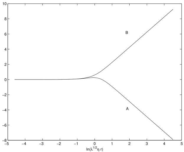
under the ansatz . Note that the coefficient for is fixed, giving the correct signature only when is negative. The coefficient is unrestricted by the Einstein equations; however, our choice to set at the origin determines . For this asymptotic metric, the scalar-field equation (10) yields asymptotic form for the monopole as
| (19) |
We display numerical solutions for and over the whole range of in Fig. 1. The appropriate asymptotic behavior is noted.
From now on we focus on inducing a four dimensional universe on the brane which is like our own. The seven dimensional theory induces an effective four dimensional theory, with Einstein equations
| (20) |
Here, barred terms are those induced by the apparent 4D metric , and is the apparent 4D cosmological constant, which includes contributions from the 7D cosmological constant, the 7D curvature , and the monopole stress-energy tensor. No term appears, as we absorb the monopole’s stress energy, diagonal in the longitudinal brane dimensions, into the effective cosmological constant . Note that our full Einstein equations (8), which told us , can be read as an effective equation for , with effective 4D cosmological constant
| (21) |
However, this detailed relationship need not be exploited. Henceforward we take the 4D background metric flat, . This results in apparent 4D Minkowski space, , with the numerical and asymptotic solutions to Einstein’s equations shown. These solutions automatically have vanishing 4D cosmological constant , because Einstein’s equations (8) are equivalent to the effective 4D equations (20), which require when .
Before we close this section, let us comment on the physical parameters in the model. The 7D Planck mass, , we take to be at the particle scale of TeV; our model solves the hierarchy problem by inducing from this natural the large effective 4D Planck mass . This leaves three free parameters, , , and . The self-coupling constant is always accompanied by to give the mass of the monopole field, . Since this mass is seven dimensional, we expect its upper bound does not exceed TeV scale. The symmetry-breaking scale is not limited; however, we confine ourselves to sub-Planckian monopoles (), which remain nonsingular at all . , which is negative for our solution, can have arbitrary magnitude.
III Graviton zero mode and Planck mass
In this section we discuss localization of the graviton zero mode. We assume a small perturbation to the background metric whose 4D part is flat. Then the metric becomes
| (22) | |||||
| (23) |
Here, gives the apparent 4D graviton field. We assume the only non-zero components of the perturbation are (). We also apply transverse-traceless gauge on , and , where the vertical bar in the subscript denotes the covariant derivative with respect to the background metric. Einstein’s equations for give
| (24) |
Here, the superscript (B) represents that the quantity is evaluated in the unperturbed background metric . With given gauge conditions on all terms but the first two cancel. Therefore, the equation for reduces to that in the curved vacuum background,
| (25) |
Equation (25) is equivalent for every component of . We thus seek solutions of the form . Equation (25) reduces to
| (26) | |||||
| (27) |
where is the d’Alembertian in flat 4D Minkowski space. We separate variables, taking . Here, determines the apparent 4D graviton mass . The angular equation
| (28) |
is solved by spherical harmonics, . This leaves the radial wave function, . Because the apparent four dimensional graviton is described by [from Eq. (23)], we solve instead for its wave function, . From Eq. (27), this satisfies
| (29) |
To determine allowed solutions and boundary conditions, we rewrite equation (29) in Sturm-Liouville form:
| (30) |
This is a Sturm-Liouville equation singular at both the origin and infinity, where regular boundary conditions must hold:
| (31) |
We seek solutions for allowed values of the eigenvalue ; for simplicity, we restrict ourselves to the case for gravitons.
We consider first the graviton zero mode, . In this case Eq. (29) is integrable, with solution
| (32) |
where and are constants. At , and . The second term in the solution becomes proportional to . It is irregular at . Even though it is normalizable, we exclude this term because of its irregular behavior at the origin. Then the only possible solution is which is a constant. This solution is regular everywhere, but is not normalizable. From the Sturm-Liouville form of the radial equation (30), the normalization weight for this zero mode solution is . Thus the graviton zero mode has normalization
| (33) |
which diverges. Physically, the origin of this divergence lies in the infinite volume of the extra dimensions.
This normalization of the zero mode is directly related to the localization of 4D gravity on the brane. When the zero mode is non-normalizable, 4D gravity cannot be realized, as the induced 4D Planck mass on the brane becomes infinite.
This effective 4D Planck mass can be calculated directly. For general , our seven dimensional theory has in its action the gravitational term
| (34) | |||||
| (35) |
Here, we have evaluated the 7D Ricci scalar , in terms of , the 4D Ricci scalar induced by , and , the 7D Ricci scalar, evaluated when is the flat 4D Minkowski metric. Viewing the term as an effective 4D gravitational action, we read off its effective coupling constant
| (36) |
after the substitution . The integral in Eq. (36) is directly proportional to the normalization of the graviton zero mode in Eq. (33). Again, this integration is divergent, making the 4D Planck mass infinite.
In the models of , the integral of Eq. (36) is finite due to the exponentially decreasing warp factor. However, in our model, the warp factor is at large and the integral diverges. Therefore, in order to have normalizable graviton zero mode and finite 4D Planck mass GeV, we introduce a cut-off. Such a cut-off should arise dynamically, due to formation of other topological defects around the monopole. It can be imposed formally, by considering a monopole and anti-monopole pair.
We estimate the cut-off radius inducing the observed hierarchy; that is, inducing 4D GeV from a 7D Planck mass of TeV scale, TeV. The main contribution to the integral in Eq. (36) comes from the region outside the core where is much larger than unity. In this region, from the result of the previous section, . Then Eq. (36) becomes
| (37) |
This gives the cut-off radius
| (38) |
where is a mass scale, undetermined because is a free parameter. However, a range of allowed parameters yield a cut-off radius acceptable by current observation. Regarding as the size of the extra dimensions in our model, gravity takes its usual 4D form so long as the separation of probe particles in the brane remains larger than . Therefore, the cut-off radius cannot not exceed 1 mm, the current observational resolution of gravitational measurement.
IV Massive Kaluza-Klein modes
In this section we discuss the massive Kaluza-Klein gravitons and their correction to the Newtonian gravitational potential on the brane.
Massive gravitons obey the radial graviton equation (30), with boundary conditions (31). This Sturm-Liouville problem for the 4D graviton wave function leads directly to two conclusions: first, the existence of the zero-mode solution examined in the previous section; and second, by standard Sturm-Liouville arguments, to positive definiteness of the allowed mass eigenvalues, , with the regular boundary conditions (31). In this form we thus see that our theory allows no tachyonic graviton modes.
To find the allowed mass eigenvalues, however, we recast the radial equation (30) as a non-relativistic Schrödinger-type equation. We rescale both the radial coordinate and the wave function by
| (39) | |||||
| (40) |
where is a constant. Then the radial equation becomes
| (41) |
with potential
| (42) |
Here, the prime denotes differentiation with respect to . Equation (41) is in the form of a Schrödinger-type equation in three dimensions, with spherically symmetric effective potential and energy eigenvalue . Therefore, the shape of the effective potential provides insight both into the allowed mass spectrum, and into how gravitons are confined in space.
However, the boundary conditions are nontrivial. Note that we must reproduce the boundary conditions (31) of the original Sturm-Liouville problem for , in order to reproduce the proper mass spectrum (eigenvalue spectrum) . These boundary conditions occur at , where , and at , where takes on the finite positive value
| (43) |
This is finite because the integrand falls as at large . These boundary conditions require that , related to by Eq. (40), must remain bounded at , or , and that
| (44) | |||||
| (45) |
where the prime again denotes differentiation with respect to . We note that the quantity in parentheses vanishes automatically for the zero mode, for which , and for no other solution. For all other modes, this quantity scales as , leading to effective regularity conditions
| (46) |
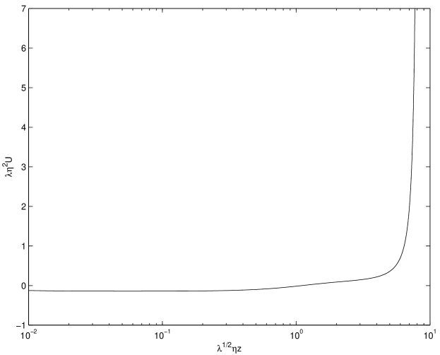
With these boundary conditions in mind, we consider our Schrödinger equation (41) with effective potential (42). Since we know the functional form for and at and , let us evaluate the functional form of and the wave function in these two asymptotic regions. The numerical plot of for the whole range is shown in Fig.2.
For small , with the aid of and in Eq. (14), we approximate . The potential reads
| (47) |
This constant potential must automatically lay below zero, as we know the zero mode, with “energy eigenvalue” , remains a solution to the transformed Schrödinger equation (41). Therefore, the wave function approaches the plane-wave solution for the given eigenvalue . To the lowest-order correction to , the solution to the wave equation (41) becomes
| (48) |
where . The cosine part is irregular at , where becomes unbounded. We thus exclude it, setting .
At large distances
| (49) |
The potential in this region becomes
| (50) |
where . As (), goes to infinity. The solution to the wave equation with this is given by
| (51) |
where . () is the Bessel function of the first (second) kind. The -function becomes irregular as , violating our nontrivial effective regularity condition (46). We thus exclude it, . From the two asymptotic behaviors of the wave function and the shape of the potential, it is clear that the wave function for the massive mode is normalizable regardless of the cut-off.
Now we are in a position to evaluate the mass spectrum. Equation (41) is in the form of a non-relativistic Schrödinger equation, whose binding potential suggests a discrete spectrum of eigenvalues. More strictly, as a Sturm-Liouville equation over the finite variable , this equation must yield discrete eigenvalues . We know, from our problem statement in radial variables, that the smallest eigenvalue is , with eigenfunction automatically obeying the regular boundary conditions (45).
Quantization of the spectrum is usually acquired by imposing regular boundary conditions on the excited eigenfunction solutions. Here, however, we know only these solutions’ asymptotic behaviors, and thus cannot impose both boundary conditions on a single candidate solution. That is, while we may discard irregular asymptotic behavior, we have no guarantee that an eigenfunction regular at the origin continues to one that is regular also at . Yet it is precisely the special case where this continuation remains regular, which determines the allowed eigenvalues .
To investigate the eigenvalue spectrum, then, we must approximate our equation (41) in such a way that a single closed-form solution connects the two asymptotic regions and . We achieve this by approximating our potential by
| (52) |
This potential approximates Eqs. (47) and (50) in the two asymptotic regions ( and ). The intermediate region is also well approximated. Even though this approximate potential is not exactly the same as the original one, we can estimate the mass eigenvalues in a good approximation. Further corrections could be found numerically by the variational method, for a specific parameter choice.
With this approximate the solution of the graviton equation (41) is
| (53) | |||||
| (54) |
Imposing our effective regularity condition (46) at excludes the -solution, . At , it forces the -solution to vanish. Thus the argument of at must be a zero of the Bessel function,
| (55) |
Here, ’s are the zeros of and is a very good approximation even for . The discrete mass spectrum is then given by
| (56) |
The mass gap between the adjacent modes is
| (57) |
The value of depends on which is given by
| (58) |
The last approximation comes after we separate the integration at beyond which we know the asymptotic and . From the above description it is clear that depends much on the parameters of the model. The estimation of is not quite possible because of the integration over the inner region.
We note that this spectrum describes the excited Kaluza-Klein modes, with . The exact mode (32) does not appear as a solution to our approximate potential (52), nor does it obey the imposed effective regularity conditions (46); although it automatically obeys the more general regularity conditions (45) transcribed directly from the radial graviton problem, Eq. (30). , with , is then the first Kaluza-Klein mode obeying the excited boundary conditions (46) , and is thus guaranteed by the Sturm-Liouville form of the original radial problem Eq. (30) to be positive. Its positiveness is not apparent from its form (56); however, self-consistency of the eigenvalue problem requires that the highly derivative quantities and must emerge with values such that .
The correction to the Newtonian potential by the massive KK gravitons is given by
| (59) |
where x is the distance between the particles of mass and in the 4D brane. For , the correction is exponentially suppressed. If (especially the lowest mode) is massive enough, the correction to the Newtonian potential will be negligable at the observational resolution, unless the KK-graviton couplings diverge.
With the wave function (54) we can evaluate these couplings of KK gravitons to the brane located at the center of the monopole, . The normalization of the wave function (54), , gives the normalization constant
| (60) |
Here, we used the relation (55) for and its definition, . Then the coupling reads
| (61) | |||||
| (62) | |||||
| (63) |
where we used the recurrence formula .
Since and emerge as such parameter-dependent quantities, let us consider the possibility of small mass gap . For small mass gap, we take the continuum limit, . The Kaluza-Klein correction to the gravitational potential is then
| (64) |
where the additional factor comes from the extra dimensional plane-wave continuum density of states, and is the unit mass. From Eqs. (55) and (63) this correction becomes
| (65) |
This correction negligibly affects the behavior of the Newtonian potential in four dimensions.
V Matter fields
In this section we investigate the effective field theory induced on the brane for 7D matter fields. Either Dirac or Klein-Gordon scalar fields obey a 7D Klein-Gordon field equation:
| (66) |
where and are the 7D field and its mass. To induce an effective 4D field, we separate variables,
| (67) |
with radial equation
| (68) |
where determines the effective 4D mass. This eigenvalue equation determines the induced 4D mass of the scalar field and its Kaluza-Klein excitations.
The radial equation is exactly the same as equation (29) for gravitons, with one more term coming from the 7D mass. Due to this additional term, for nonzero, no zero-mode type solution exists. However, we may recast this equation to the Schrödinger-type equation (41) by the same transformations (39) and (40). The potential for the KG-wave equation is then given by
| (69) |
Therefore, the potential is corrected from the graviton potential by adding a term with the 7D mass. At small it asymptotes to
| (70) |
and at large it goes to
| (71) |
Then the properties of the potential and the wave function are the same with those for massive gravitons after we substitute two constants and with and . The localization behavior is the same as that of massive KK gravitons. Therefore, we have a 4D KG field localized on the brane, with discrete mass spectrum , for .
VI conclusions
We investigated the brane physics induced by a global monopole formed in three extra dimensions. The metric induced by the monopole background, with negative cosmological constant, makes the volume of the extra dimensions infinite. As usual in models of infinite extra dimensional volume, the graviton zero mode is not normalizable without a cut-off. We view a cut-off as physically natural, due to formation of adjacent defects during the dimension-reducing phase transition, and choose the cut-off radius to induce a hierarchical 4D Planck mass (GeV) from a unified 7D Planck mass (TeV). We have a possible range of parameters to make this cut-off radius (size of extra dimensions) consistent with current observations.
Our model admits a discrete spectrum of massive Kaluza-Klein gravitons. These massive modes are not harmful to 4D gravity on the brane, whether the mass gap is large or small.
Recently it was suggested that 4D gravity can be induced by the massive KK gravitons even when the zero mode is not normalizable [12]. Four dimensional gravity in that scenario is viable in the intermediate length scale. The induced graviton is meta-stable on the brane and decays to the bulk at a finite life time. Therefore, at a large scale higher dimensional gravity applies. The scenario is still under dispute. However, it will be challenging to examine its validity in our model in which the zero mode is not naturally normalizable.
In addition to gravitons we found that 7D matter fields can induce 4D matter fields on the brane. The localization picture is very similar to that of massive gravitons. It will be interesting to study the effective field theory of matter interactions on the brane, and the resultant brane cosmology.
Acknowledgements.
We are grateful to Gia Dvali, Alex Vilenkin, Takahiro Tanaka, and Gaume Garriga for helpful discussions. I.C. also acknowledges Chi-Ok Hwang. This work was supported by the University Research Committee of Emory University.REFERENCES
- [1] T. Kaluza, Preus. Acad. Wiss. K 1, 966 (1921); O. Klein, Zeit. Phys. 37, 895 (1926).
- [2] N. Arkani-Hamed, S. Dimopoulos and G. Dvali, Phys. Lett. B 429, 263 (1998); Phys. Rev. D 59, 086004 (1999).
- [3] L. Randall and R. Sundrum, Phys. Rev. Lett. 83, 3370 (1999); ibid. 4690 (1999).
- [4] V. Rubakov and M. Shaposhnikov, Phys. Lett. B 125, 139 (1983).
- [5] V. Rubakov and M. Shaposhnikov, Phys. Lett. B 125, 136 (1983).
- [6] G. Dvali and M. Shifman, Phys. Lett. B 396, 64 (1997).
- [7] I. Olasagasti and A. Vilenkin, Phys. Rev. D 62, 044014 (2000).
- [8] A. Cohen and D. Kaplan, Phys. Lett. B 470, 52 (1999).
- [9] R. Gregory, Phys. Rev. Lett. 84, 2564 (2000).
- [10] T. Gherghetta and M. Shaposhnikov, Phys. Rev. Lett. 85, 240 (2000).
- [11] T. Gherghetta, E. Rossel and M. Shaposhnikov, Phys. Lett. B 491, 353 (2000).
- [12] R. Gregory, V. Rubakov and S. Sibiryakov, Phys. Rev. Lett 84, 5928 (2000); Phys. Lett B 489, 203 (2000); C. Csaki, J. Erlich and T. Hollowood, Phys. Rev. Lett. 84, 5932 (2000); Phys. Lett. B 481, 107 (2000); G. Dvali, G. Gabadadze and M. Porrati, Phys. Lett. B 484, 112 (2000); ibid. 129 (2000).