Abstract

We obtain a solution describing a gravitational shockwave propagating along a Randall-Sundrum brane. The interest of such a solution is twofold: on the one hand, it is the first exact solution for a localized source on a Randall-Sundrum three-brane. On the other hand, one can use it to study forward scattering at Planckian energies, including the effects of the continuum of Kaluza-Klein modes. We map out the different regimes for the scattering obtained by varying the center-of-mass energy and the impact parameter. We also discuss exact shockwaves in ADD scenarios with compact extra dimensions.

1 Introduction

No matter how small the rest mass of a particle is, when it is accelerated to energies in or above the Planck scale its gravitational field becomes so strong that it can not be neglected. It has been known for some time what this field looks like: a planar shock wave, whose rays propagate parallelly to the direction of motion [1, 2]. When another particle crosses this wavefront, its trajectory is altered—in other words, the second particle is scattered by the attractive gravitational field of the Planckian-energy particle. It was shown in [3] that the amplitude for this sort of scattering can be exactly calculated. As it turns out, this way of computing the scattering between the two particles corresponds to the leading approximation to the forward scattering of two particles in quantum gravity, for center-of-mass energy much larger than the momentum transfer [4, 5, 6, 7, 8, 9].

It has been commonly assumed that, given the enormous value of the Planck scale, Planckian energies would very hardly be attainable. However, it has been realized in recent years that the fundamental scale for quantum gravity may not be the usual four-dimensional Planck scale, $M_{Pl}\sim 10^{18}$ GeV. Rather, the fundamental scale $M_{*}$ might be essentially anywhere between the TeV scale and $M_{Pl}$. The latter would be a derived magnitude, adequate for describing gravity only at low energies/large distances, and its large value would arise as a consequence of the existence of large (ADD [10]), or warped (RS1 [11]), extra dimensions. If some form of scenario of low-scale quantum gravity were actually realized, Planckian energies might be much more accesible than previously thought. For $M_{*}$ in the TeV range, it could be reached in colliders in the near future, whereas intermediate, as well as low, scales might perhaps be probed by extreme energy cosmic rays. Currently, the case for the latter is still open, see e.g., [12], but it should be noted that the regime probed by these cosmic rays appears to be precisely the one described in the previous paragraph.

Given these considerations, it is natural to try to extend the analysis of the shockwave of an ultra-high-energy particle to such scenarios with extra dimensions. Among these, a large and particularly interesting class regards our universe as a three-brane embedded in a higher dimensional bulk [13, 14, 10, 11, 15]. The focus of this paper will be on such brane-world scenarios, and, mostly, on the Randall-Sundrum model with an infinite extra dimension [15], henceforth RS2.

The phenomenology of RS2 is not as much developed as that of ADD or RS1. Some steps were taken in [16]. The main difference is that RS2 is not designed to address the hierarchy problem. In fact, in RS2 the fundamental and effective four-dimensional gravity scales are related as $M_{*}=(M_{Pl}^{2}/\ell)^{1/3}$, and since experiment bounds $\ell$—the curvature scale of the extra dimension—to be not larger than 1 mm, then $M_{*}>10^{5}$ TeV, which still might be within the reach of cosmic rays. Nevertheless, there are variants of RS2 [17] with $n$ extra dimensions which allow for much lower values of $M_{*}$ through $M_{*}=(M_{Pl}^{2}/\ell^{n})^{1/(n+2)}$. We will focus exclusively on RS2, but the extension of our analysis to the models of [17] should not present technical difficulties.

From the conceptual point of view, the RS2 model has resulted extremely fruitful, opening up new avenues for thinking about gravity in extra dimensions. However, the structure of the model—a three-brane in a constant negative curvature background—has made it very difficult to analyze gravity on it in an exact way. It is particularly important to know what is the gravitational field created by sources localized to the brane. So far, the only known exact solutions, constructed in [18], describe black holes in a lower-dimensional setting—a two-brane in a four-dimensional bulk. Hence, the construction of other simple, exact solutions in this model is of obvious interest. A main part of this paper (Section 2) is devoted to constructing the exact gravitational shockwave of an effectively massless particle within the RS2 model. To our knowledge, these are the first exact solutions to describe the gravitational field of a localized source on a RS brane in $AdS_{5}$ (or higher dimensions). With this solution in hand, we will follow [3] and [5] in Section 3 to describe certain aspects of Planckian scattering on the brane.

Finally, given their phenomenological interest, one would also like to have a similarly exact description of shockwaves in ADD scenarios. If the gravitational backreaction of the brane is neglected (as it usually is, but see [19]), this turns out to be much easier than in the RS2 model. Therefore, we will present these solutions in Section 4.

Throughout this paper we will denote the conventional (four-dimensional) Planck mass as $M_{Pl}\equiv G_{4}^{-1/2}$, while $M_{*}=G_{5}^{-1/3}$ will be the fundamental (five-dimensional) mass. What is precisely meant by ‘Planckian energy’, and in which regime, will be discussed in Section 3. We also take $\ell$ to be larger than the fundamental (or string) scale. This seems reasonable, since otherwise the semiclassical description of the RS setup using Einstein gravity would not be reliable.

2 Gravitational Shockwave on the RS Brane

Working in an arbitrary number of dimensions, the RS2 scenario describes a $(d-1)$-brane in the $AdS_{d+1}$ spacetime, the case of most relevance being obviously $d=4$. The ground state metric is

$$ds^{2}=dy^{2}+e^{-2|y|/\ell}\eta_{\mu\nu}dx^{\mu}dx^{\nu}\,,$$ (1)

with $\mu,\nu=0,\dots,d-1$. The coordinate $y$ measures the proper distance transverse to the brane, which is itself located at the orbifold point $y=0$. It is at times also convenient to use another form for the metric, by changing the bulk coordinate to

$$z=\ell(e^{y/\ell}-1)\,,$$ (2)

so

$$ds^{2}={\ell^{2}\over(\ell+|z|)^{2}}(dz^{2}+\eta_{\mu\nu}dx^{\mu}dx^{\nu})\,.$$ (3)

The brane is now at $z=0$.

Our starting point is a particle at rest on the brane. In Ref. [1], Aichelburg and Sexl showed that, in four flat dimensions, the metric for the shockwave could be constructed by performing a boost to the speed of light on the Schwarzschild solution. In the present case, exact solutions for black holes on RS branes in $AdS_{d+1}$ are unknown except for the low-dimensional model in $d=3$ [18]. We will instead use the approximations that have been constructed up to linearized order. As in the case of [1], performing an ultrarelativistic boost will have the effect that only the linearized part of the solutions remains important.

Therefore, let us place a source on the brane, localized on it, which means that its stress-energy tensor $t_{\mu\nu}(x)$ has components only along the brane-world indices, and that it depends solely on the brane-world coordinates. The equations for the linearized perturbation $\eta_{\mu\nu}+h_{\mu\nu}$ induced by the source have been the subject of a number of papers, including [15, 20, 21, 22]. The final result can be given in terms of Fourier transforms with respect to the brane-world coordinates,

$$h_{\mu\nu}(q,y)=\int d^{4}x\;e^{-iq_{\sigma}x^{\sigma}}h_{\mu\nu}(x,y)\,,$$ (4)

in the form [22]

$$\tilde{h}_{\mu\nu}(q,y)=8\pi G_{d+1}\left[t_{\mu\nu}(q)-{1\over d-1}\left(\eta_{\mu\nu}-{q_{\mu}q_{\nu}\over q^{2}}\right)t\right]e^{d|y|\over 2\ell}{K_{d/2}(e^{|y|/\ell}\ell q)\over qK_{d/2-1}(\ell q)}\,.$$ (5)

The tilde denotes the tracefree perturbation $\tilde{h}_{\mu\nu}=h_{\mu\nu}-{1\over d}\eta_{\mu\nu}h$, and the solution is expressed in terms of Bessel $K_{\nu}$ functions. Also, $G_{d+1}=M_{*}^{-d+1}$ is the $d+1$ dimensional gravitational constant. The trace of the perturbation must satisfy

$$h|_{y=0}=-{32\pi G_{d+1}\over(d-1)\ell q^{2}}t\,,$$ (6)

but in fact we will not need it.

For a point particle at rest, of mass $m$, the stress-energy tensor is $t_{00}(q)=2\pi m\delta(q_{0})$. The corresponding metric perturbation can be readily found from the above formulas, even if the inverse Fourier transforms can only be explicitly evaluated in certain limits. Nevertheless, we can still boost the solution in Fourier space. When boosted to high energies the particle becomes ultrarelativistic, and then we can effectively take $v\to 1$, while keeping the momentum $p=\gamma mv$ fixed. Instead of boosting the solution $h_{\mu\nu}$ for a particle at rest, we will, equivalently, find the solution that corresponds to the stress-energy tensor of a boosted particle. This stress-energy tensor transforms under the boost, and then as $v\to 1$, as

$$t_{00}(q) = 2\pi\gamma m\;\delta(q_{0}+vq_{1})\to 2\pi p\;\delta(q_{0}+q_{1})\,,$$

$$t_{01}(q) = vt_{00}(q)\to t_{00}(q)\,,$$ (7)

$$t_{11}(q) = v^{2}t_{00}(q)\to t_{00}(q)\,,$$

which is effectively the stress-energy tensor of a massless particle. We can now plug this into equation (5) to obtain the desired form of the solution. It is important to note that the stress-tensor (2) is trace-free. Hence the metric perturbation $h_{\mu\nu}$ can be taken to be trace-free too. This implies that the so-called “brane-bending” effect [20] is absent. The gravitons with polarizations transverse to the brane are not excited and hence the brane does not bend into the bulk.

Given that we are dealing with a limiting lightlike source, it is convenient to work with the light-cone coordinates $u=t-x$, $v=t+x$. In terms of these, the perturbed metric for a null source takes the form

$$ds^{2}=dy^{2}+e^{-2|y|/\ell}(-dudv+dx^{i}dx^{i}+h_{uu}(u,x^{i},y)du^{2})\,,$$ (8)

where $i=2,\dots,d-1$ labels the coordinates in the brane-directions transverse to the propagation. Plugging the stress-energy tensor

$$t_{uu}=2\pi p\;\delta(q_{0}+q_{1})\,,$$ (9)

into (5), and transforming back to coordinate space we get

$$h_{uu}(u,x^{i},y)={4G_{d+1}\over(2\pi)^{d-3}}p\;\delta(u)e^{d|y|\over 2\ell}\int d^{d-2}q_{i}\;e^{iq_{i}x^{i}}{K_{d/2}(e^{|y|/\ell}\ell q)\over qK_{d/2-1}(\ell q)}\,,$$ (10)

where now $q=|q_{i}q_{i}|^{1/2}$ is the modulus of the projection of $q_{\mu}$ on the plane transverse to the propagation of the particle, i.e., parallel to the wavefront. The Fourier transforms cannot, for $d\geq 4$, be carried out fully explicitly, but at least the angular integrations that appear can be performed,

$$h_{uu}(u,r,y)={4G_{d+1}\over(2\pi)^{d-4\over 2}}p\;\delta(u){e^{d|y|\over 2\ell}\over r^{d-4\over 2}}\int_{0}^{\infty}dq{q}^{d-4\over 2}J_{d-4\over 2}(qr){K_{d/2}(e^{|y|/\ell}\ell q)\over K_{d/2-1}(\ell q)}\,,$$ (11)

where $r$ is the radial distance on the wavefront on the brane, transverse to the direction of propagation of the particle. Note that away from the wavefront, the perturbation vanishes.

This solution is in fact an exact one: for a $d+1$-dimensional metric of the plane wave form (8) the exact Einstein tensor is

$$G_{yy} = {d(d-1)\over 2\ell^{2}}g_{yy},$$

$$G_{\mu\nu} = \left({d(d-1)\over 2\ell^{2}}-{2(d-1)\over\ell}\delta(y)\right)g_{\mu\nu}-{1\over 2}\partial_{\mu}u\partial_{\nu}u\left[e^{-2|y|/\ell}\left(\partial^{2}_{y}-{d\over\ell}\partial_{y}\right)+\nabla^{2}_{x}\right]h_{uu}\,.$$ (12)

All other components vanish. This exact Einstein tensor is linear in $h_{uu}$. Hence by solving the equations at linearized order we have actually solved them to all orders. This linearization, which had been noted earlier in [23], allows to construct exact plane waves localized on the brane in the RS model.

Therefore, the solutions (11) provide an exact description of the gravitational field of a lightlike point source localized on the brane.

Let us now focus on the case of $d=4$, and in particular, on the metric at the location of the brane, $y=0$. Although we have not been able to perform the last integration in (11) explicitly, we can approximate it in several limits. At large distances from the source on the wavefront on the brane, $r\gg\ell$, we can expand the Bessel functions for small $q$, to find

$$h_{uu}=-4G_{4}p\;\delta(u)\left[\log(r^{2}/\ell^{2})-{\ell^{2}\over r^{2}}+{2\ell^{4}\over r^{4}}\left(\log(r^{2}/\ell^{2})-1\right)+\dots\right]\,.$$ (13)

This result has been written already in terms of the effective gravitational coupling constant induced on the brane, $G_{4}=G_{5}/\ell$. As was the case for static point masses, the first correction, $\sim-\ell^{2}/r^{2}$, does not resemble the profile of a five-dimensional shockwave (which would go like $\ell/r$), rather that of a six-dimensional one. However, at short distances ($r^{2}+y^{2}\ll\ell^{2}$), instead, it is easy to see that the five dimensional form of the shockwave is recovered, due to dominance of KK modes. More explicitly, on the brane at $r\ll\ell$,

$$h_{uu}=-4G_{4}p\;\delta(u)\left[-{\ell\over r}+{3\over 2}\log(r/\ell)+{3r\over 8\ell}+\dots\right]\,.$$ (14)

A different form for the solution, which is better suited for numerical evaluation of the integrals, can be obtained by applying the analysis in [20] to the source of (9):

$$h_{uu}(u,r,y)= -4G_{4}p\;\delta(u)\biggl{[}e^{-2|y|/\ell}\log(r^{2}/\ell^{2})$$ (15)

$$-{2\ell\over\pi}\int_{0}^{\infty}dm\;K_{0}(mr){Y_{1}(m\ell)J_{2}(m\ell e^{|y|/\ell})-J_{1}(m\ell)Y_{2}(m\ell e^{|y|/\ell})\over J_{1}^{2}(m\ell)+Y_{1}^{2}(m\ell)}\biggr{]}\,.$$

The zero mode term has been split from the continuum of Kaluza-Klein modes of mass $m$. Again, this is an exact form for the solution. The factor $e^{-2|y|/\ell}$ indicates the suppression of the solution into the bulk. On the brane the solution becomes

$$h_{uu}(u,r,y=0)=-4G_{4}p\;\delta(u)\left[\log(r^{2}/\ell^{2})-{4\over\pi^{2}}\int_{0}^{\infty}{dm\over m}{K_{0}(mr)\over J_{1}^{2}(m\ell)+Y_{1}^{2}(m\ell)}\right]\,.$$ (16)

We have used this latter form of the solution to plot $h_{uu}(r)$ in Fig. 1. The figure very clearly shows how the Kaluza-Klein modes introduce, at distances $r<\ell$, an enhancement of the gravitational shockwave relative to the zero-mode truncation, i.e., the leading log term in (13) and (16). In Fig. 2 we exhibit how the exact solution interpolates between the four-dimensional behavior at large distances, and five-dimensional gravity at short distances. In the latter case, it is interesting to note that the leading order approximation, $1/r$, yields a weaker effect than the exact value. The first correction in (14), $\sim-3\log(r/\ell)/2$, becomes in fact of some importance.

Figure 1: Log-scale plot of the profile of the shockwave $h_{uu}(r)$ on the RS three-brane. It clearly exhibits the deviation, due to the Kaluza-Klein modes, from the four-dimensional logarithmic solution (dotted line). The units for $r$ are such that $\ell=1$.

Figure 2: The shockwave profile $h_{uu}(r)$ on an RS three-brane (solid line). It interpolates between the leading order behaviors at short distance ($\sim r^{-1}$) and large distance ($\sim-\log r$), in dotted lines. Again, we have set $\ell=1$.

The shockwave on a two-brane

It is interesting to consider separately the low-dimensional case of $d=3$, corresponding to a domain wall in $AdS_{4}$. For the shock wave solution all the calculations can be carried out explicitly to the end, since the Bessel functions involved can be finitely expressed in terms of elementary functions. Using the form of the metric in terms of the $z$ coordinate of (3) we find

$$h_{uu}=-4G_{4}p\;\delta(u)\left(\log(r^{2}+z^{2})+{2|z|\over\ell}+{2r\over\ell}\arctan{r\over|z|}\right)\,.$$ (17)

Along the brane at $z=0$ this reduces to

$$h_{uu}(u,r,z=0)=-8G_{3}p\;\delta(u)\left(\pi|r|+\ell\log(r^{2})\right)\,,$$ (18)

where we have used $G_{4}=2\ell G_{3}$. As explained above, the linearized solution is in fact an exact one. As was the case for black holes on a two-brane constructed in [18], the exact metric on the brane (18) is precisely the sum of the $2+1$ dimensional ($\propto|r|$) and $3+1$ dimensional ($\propto\log(r^{2})$) solutions. Observe that in the bulk of spacetime, the four-dimensional form of the solution ($\sim\log(r^{2}+z^{2})$) is recovered for small $r$ and $z$.

In [2] it was shown how the Aichelburg-Sexl solution can be constructed by a cut-and-paste method performed in flat Minkowski space. It would be interesting to show how this exact solution is obtained by similarly cutting and pasting patches of $AdS_{4}$ (see [24] for possibly related work).

3 Planckian Scattering on the Brane

We will now study the elastic forward scattering amplitude, in a regime where the center-of-mass energy is at a very large scale, and is much larger than the momentum transfer, $s/|t|\gg 1$. Gravitons are expected to dominate over other interactions above the Planck energy. Obviously, one must specify what is meant by ‘Planckian energies’ here, i.e., whether $E>M_{*}$ or $E>M_{Pl}=M_{*}\sqrt{M_{*}\ell}\gg M_{*}$. Recall that the assumption of ‘Planckian center-of-mass energies’ has several motivations. First, it ensures that the rest mass $m_{0}$ of the particle is negligible. To this effect, we just need energies $E\gg m_{0}$, but not necessarily Planckian. More importantly, at energies above the Planck scale the effective dimensionless coupling $\alpha_{G}\equiv s/M_{Pl}^{2}$ becomes large and gravity is expected to be strongly coupled. Furthermore, due to the growth of this coupling with energy, it will dominate over any other interactions. In the present case, however, one should consider first the distance scale that is being probed. If the impact parameter $b$ is much larger than $\ell$, then the graviton zero-mode dominates over KK modes. In this regime, Planckian energy will necessarily mean $E>M_{Pl}$. The graviton zero-mode will then be strongly coupled. Instead, for $b<\ell$ the KK modes dominate and the interaction becomes five-dimensional. Here our methods can also be applied to the regime of $M_{*}<E<M_{Pl}$, but this will not necessarily imply that the KK modes are strongly coupled—we will discuss when they are. Gravity need not dominate over other interactions in this regime. But for $E>M_{Pl}$ five-dimensional gravity will always be strongly coupled.

The forward scattering of two particles (or strings) at Planckian energies has been studied in the past [3, 4, 5], however, the possibility of new dimensions opening up was not generally considered. Some discussion of this point has been given in [25]. Our analysis is somewhat complementary to that in [25], but we will go into more detail at several points. From the technical point of view, we mainly build up on the work of [3] and [5, 6]. The regime of Planckian energies and large $s/|t|$ can be treated in the eikonal approximation—a resummation of an infinite number of graviton ladder and cross-ladder diagrams, which dominates the elastic forward scattering. Although it resums contributions from all orders in the coupling constant, this approximation does not actually probe quantum gravity effects. Effectively, graviton loops are suppressed if the impact parameter $b$ is much larger than the fundamental length $M_{*}^{-1}$ (the momentum exchanged by each graviton is much less than $M_{*}$). Hence, corrections in $1/(bM_{*})^{2}$ are neglected. Notice also that four-dimensional graviton loops are suppressed by the much larger factor $1/(bM_{Pl})^{2}$.

Another important point is the possibility of black hole physics entering at impact parameters of the order of the Schwarzschild radius associated to a given center-of-mass energy. Precise calculations are way beyond any computational scheme available (it involves tree-level graviton exchange to all orders, and possibly beyond perturbation theory), but we will discuss this later in mostly qualitative terms.

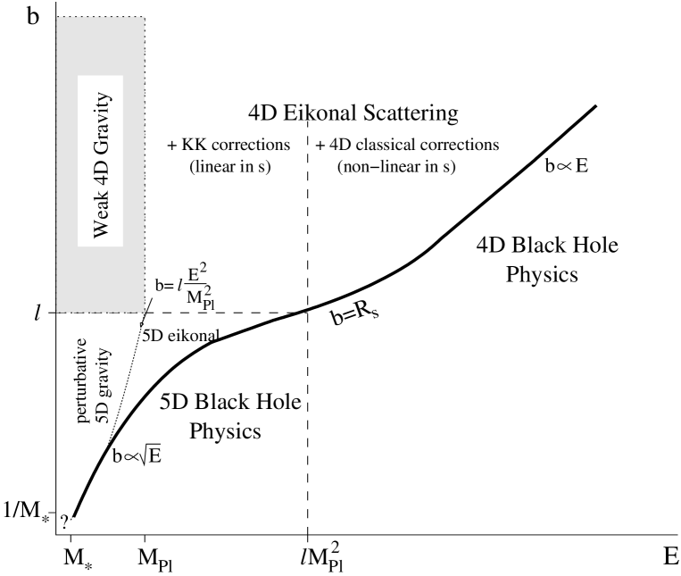
Figure 3: The different regimes for the scattering at energies $E>M_{*}$ and impact parameters $b>1/M_{*}$. The boundaries between regimes are merely indications of where the crossover from one behavior to another takes place.

Following [3] (see also [26]) the shockwave geometry directly yields the relevant information needed to compute the eikonalized gravitational scattering amplitude for two particles at large center of mass energy $\sqrt{s}=2E$. Let $a(s,b)$ be the scattering amplitude expressed as a function of the impact parameter $b$. In eikonal form

$$a(s,b)=e^{2i\delta(s,b)}\,.$$ (19)

If we identify the impact parameter $b$ with the distance in the direction transverse to the propagation of the shockwave, $b=\sqrt{x^{i}x^{i}}$, then $\delta(s,b)$ can be read off from the shockwave metric as

$$h_{uu}=8p\;\delta(u){\delta(s,b)\over s}\,.$$ (20)

Having $a(s,b)$, one can compute the amplitude for a given momentum transfer, $t=-q_{i}q_{i}=-|q|^{2}$, by transforming

$${1\over s}a(s,t) = {2\over i}\int d^{2}x\;e^{iq_{i}x^{i}}\left(e^{2i\delta(s,b)}-1\right)$$ (21)

$$= {4\pi\over i}\int_{0}^{\infty}db\;bJ_{0}(bq)e^{2i\delta(s,b)}\,.$$

It is important to notice here that the Fourier transform is a two-dimensional one, even if the shockwave front is three-dimensional. The reason is that we are considering the scattering of particles confined to the brane, and therefore the impact parameter is restricted to the two transverse directions along the brane. The available phase space is reduced in comparison to particles that propagate freely in the bulk. As a consequence, even at short distances $b\ll\ell$ the scattering amplitude $a(s,t)$ will differ from the “really five-dimensional” one.

Let us first consider impact parameters $b$ larger than $\ell$. In this regime, which is essentially four-dimensional, the eikonal approach is only justified if $E>M_{Pl}$, and not for $M_{*}<E<M_{Pl}$. At $b>\ell$ and energies below $M_{Pl}$, the gravitational interaction is very weak and likely to be dominated by other interactions. But for $E>M_{Pl}$ gravitons dominate and we can obtain the eikonal from (13) and (20). Keeping only the two first terms, we get

$$\delta(s,b)=-G_{4}s\left(\log(b/\ell)-{\ell^{2}\over 2b^{2}}\right)\,.$$ (22)

The KK correction to the leading logarithmic term,

$$\delta_{KK}(s,b)=G_{4}{s\ell^{2}\over 2b^{2}}\,,$$ (23)

grows linearly with $s$, just like the four-dimensional term, a fact that distinguishes it from other non-linear corrections. The expansion parameter for KK corrections is $\ell^{2}/b^{2}$. Classical corrections to the eikonal, that include the graviton self-interaction vertices, but still at graviton tree level, have the expansion parameter $G_{4}^{2}s/b^{2}=s/(M_{Pl}^{2}b^{2})$ [6]. Since we are assuming that $M_{Pl}\gg\ell^{-1}$, then the KK corrections will be larger than these 4D classical corrections up to energies $E\sim M_{Pl}^{2}\ell$.

With (22), the integral (21) can be evaluated at a saddle point $b=b_{s}$ such that

$$q=-2{\partial\delta(s,b)\over\partial b}|_{b_{s}}\\ \simeq{2G_{4}s\over b_{s}}\left(1+{\ell^{2}\over b_{s}^{2}}\right)\,.$$

As long as the saddle point satisfies $b_{s}>\ell$, it is justified to ignore the physics at smaller $b$ in the integral (21). Notice that the momentum exchanged at a given impact parameter is larger than in four dimensions, due to the exchange of KK modes. Equivalently, the deflected angle,

$$\theta\simeq 2\sqrt{-t\over s}\simeq{4G_{4}E\over b_{s}}\left(1+{\ell^{2}\over b_{s}^{2}}\right)\,,$$ (24)

is increased, showing the extra attraction that KK modes induce.

Let us now move to the short distance regime $b<\ell$. In this case, keeping just the leading order from (14) one gets

$$\delta(s,b)\simeq{G_{4}s\ell\over 2b}\,.$$ (25)

This eikonal phase is small if $2b>G_{4}s\ell=s/M_{*}^{3}$, and therefore leads to a perturbative regime, which, for the fixed $t$ amplitude, is at momentum transfer $q<2/(G_{4}s\ell)$. This is, the Born term dominates the expansion, and one can do without the eikonal resummation. This is in contrast to the previous situation, where the amplitude was always non-perturbative, and dominated by a saddle point. Gravity here is five-dimensional (it involves all the KK modes), and the interaction is stronger than it would be in a four dimensional setup. But it is not strongly coupled.

Starting at fixed energy $M_{*}<E<M_{Pl}$, one enters this regime when the impact parameter gets below $\ell$. The fixed-$t$ amplitude becomes

$$a(s,t)\simeq 8\pi s\int_{0}^{\infty}db\;bJ_{0}(bq)\delta(s,b)=4\pi G_{4}\ell\;{s^{2}\over q}\,.$$ (26)

This is different from the usual perturbative result for gravity, which is (in any dimension) $\sim G_{n}s^{2}/q^{2}$. The reason has been explained above: although the interaction is five dimensional, the scattered particles are confined to the four-dimensional brane.

For $q>2/(G_{4}\ell s)$ we enter a strong coupling regime and the amplitude $a(s,t)$ is again dominated by a saddle point, this time at

$$q\simeq{G_{4}s\ell\over b_{s}^{2}}\,.$$ (27)

In this case the full eikonal resummation is relevant, and the amplitude evaluated at the saddle point is

$$a(s,t)\simeq 4\pi\sqrt{G_{4}\ell\over 2}\left({s\over q}\right)^{3/2}e^{2i\sqrt{G_{4}\ell sq}-i\pi/2}\,.$$ (28)

The non-analytic dependence on the coupling shows the non-perturbative character of the amplitude.

Let us note that the ’t Hooft poles [3] do not appear in these amplitudes. When the eikonal phase is purely logarithmic (i.e., 4D), these poles arise from the $b\to 0$ region in the integral (21). Here, however, the eikonal changes from 4D behavior to 5D behavior before getting to $b\to 0$, and the poles disappear. Since the ’t Hooft poles could be interpreted as a remnant of the bound states in the 4D Coulomb potential [7, 9, 27], it is no surprise that they are absent here, since the 5D Coulomb potential does not have (stable) bound states.

The results above cease to be reliable when the impact parameter becomes of the order of, or smaller than the gravitational (Schwarzschild) radius, $R_{s}$. Indeed, for $b\ll R_{s}$ one expects gravitational collapse to take place. The details, though, are expected to be very complicated, particularly for intermediate scales $b\sim R_{s}$. Although the full scattering problem is way beyond the techniques used here (see [28]), one can assume this regime will be dominated by black hole physics. Hence the discussion will be at a qualitative level. Additional discussion of related issues can be found in [29].

In a scenario like this, the Schwarzschild radius $R_{s}$ changes depending on the regime one is in. In the effective four dimensional regime of distances larger than $\ell$, the classical gravitational radius is

$$R_{s}\simeq 2G_{4}E\,.$$ (29)

The black hole is a ‘pancake’ in this regime, with a very small extent into the bulk $\sim\ell\log(R_{s}/\ell)\ll R_{s}$ [18, 21]. The physics of these black holes is described by four-dimensional laws. Instead, at distances shorter than $\ell$,

$$R_{s}\simeq\sqrt{8G_{5}E\over 3\pi}=\sqrt{8G_{4}\ell E\over 3\pi}\,.$$ (30)

These small black holes are roughly spherical in five dimensions. The growth with $E$ changes from one regime to the other, with some smooth interpolation at distances $\sim\ell$.

The total cross section for producing these black holes can be estimated to be of the order of the corresponding black hole area. Depending on whether the black hole is a large or a small one, we have

$$\sigma \sim {s\over M_{Pl}^{4}}\qquad\mathrm{for}\ E>\ell M_{Pl}^{2}\,,$$

$$\sigma \sim {\sqrt{s}\over M_{*}^{3}}={\ell\sqrt{s}\over M_{Pl}^{2}}\qquad\mathrm{for}\ E<\ell M_{Pl}^{2}\,.$$ (31)

Since the particles scatter on the brane, the relevant magnitude for producing a small black hole is not the five-dimensional black hole area (which is in fact a volume), but rather its section along the brane, which can be assumed to be along an equator of the horizon. Notice also that an effectively four-dimensional black hole will not be formed until $E>M_{Pl}^{2}\ell\gg M_{Pl}$.

The black holes thus created will evaporate by emission of Hawking radiation. In either regime (large or small), the radiation will be emitted mostly along the brane [18, 30].

The different regimes in the $(E,b)$ plane are displayed in Figure 3. The region marked “weak 4D gravity” is one where four-dimensional gravity is weakly coupled and the interaction dominated by single graviton exchange, which we have not discussed here—the leading amplitude is the same as the eikonal, up to a phase. The regions labelled “eikonal” are ones where gravity is strongly coupled, and the full eikonal resummation of the amplitude is needed. The amplitudes are non-perturbative there. The curve $b=R_{s}$ is an interpolation between (29) and (30). Note that the scattering is directly sensitive to the extra dimensions only at energies below $\ell M_{Pl}^{2}$. Going to higher energies does not actually lead into five-dimensional physics.

The picture should be valid down to impact parameters $b>1/M_{*}$ (or the string length), where new physics takes over. This regime is beyond the techniques used here.

4 Exact Shockwaves in the ADD scenario

The construction of exact shockwaves in ADD scenarios is simpler than in RS. We discuss it briefly here.

The ADD scenario consists of a three-brane (admitting a Poincaré-invariant vacuum) living in a $4+n$-dimensional spacetime. In the most basic setup, the bulk is empty and the gravitational backreaction of the brane is neglected: the brane is simply a $3+1$ hypersurface embedded in the bulk. The extra dimensions are supposed to be compactified on a certain manifold $\mathcal{M}$. If the bulk is empty, then the metric on $\mathcal{M}$ has to be Ricci-flat. Hence, if we label the brane coordinates by $x^{\mu}$, and the transverse coordinates by $y^{a}$, the vacuum is

$$ds^{2}=\eta_{\mu\nu}dx^{\mu}dx^{\nu}+\hat{g}_{ab}\;dy^{a}dy^{b}\,,$$ (32)

where $\hat{g}_{ab}$ is the metric on $\mathcal{M}$, and the brane is at a certain point in $\mathcal{M}$, say, at $y^{a}=0$.

The linearization of the Einstein equations that occurs for the solutions we seek simplifies again the construction. A plane-fronted wave will be of the form

$$ds^{2}=-dudv+dx^{i}dx^{i}+h_{uu}(x,y)du^{2}+\hat{g}_{ab}dy^{a}dy^{b}$$ (33)

($i=2,3$). For a lightlike source localized on the brane the Einstein equations become

$$(\nabla^{2}_{x}+\nabla^{2}_{y})h_{uu}(x,y)=-16\pi G_{4+n}t_{uu}(x)\delta^{(n)}(y)\,,$$ (34)

where we have split the Laplacian operator in the wavefront into the brane $\nabla^{2}_{x}$ and the bulk $\nabla^{2}_{y}$ parts. The problem is now a rather standard one. As in the RS case, a way to solve this equation is by first Fourier-transforming the brane coordinates,

$$(-q^{2}+\nabla^{2}_{y})h_{uu}(q,y)=-16\pi G_{4+n}t_{uu}(q)\delta^{(n)}(y)\,,$$ (35)

One now needs the (massive Euclidean) Green’s function in the transverse bulk space,

$$(-q^{2}+\nabla^{2}_{y})G(q,y)=\delta^{(n)}(y)\,.$$ (36)

For the null pointlike source (9), the solution is then

$$h_{uu}(u,x^{i},y)=-16\pi G_{4+n}p\;\delta(u)\int{d^{2}q\over(2\pi)^{2}}e^{iq_{i}x^{i}}G(q,y)\,,$$ (37)

which is the analogue of (11). Obviously, one can as well give the solution as an analogue of (15) by finding the eigenfunctions of the operator in (36). As remarked above, it is the linearized character of the equations which allows to perform the entire construction. The main problem lies in calculating the Green’s function (36) in the extra space.

For an illustration, consider the case where the extra dimensions are compactified on a torus $T^{n}$. Then, instead of (37), the solutions are most easily obtained by using the method of images, i.e., by constructing a periodic array of $4+n$ dimensional shockwaves. Since the equations are linear, one simply superimposes the individual solutions. If, for simplicity, the torus is a square one, $y^{a}\sim y^{a}+L$, then standard manipulations yield

$$h_{uu}(u,r,y)=-4G_{4}p\;\delta(u)\left[\log(r^{2})-2{\sum_{n_{a}\in\mathbf{Z}^{n}}}^{\prime}K_{0}(m_{n}r)e^{-in_{a}y^{a}/L}\right]\,,$$ (38)

where the sum is over vectors $n_{a}$ on a square lattice excluding the origin (the zero mode has been split already), and $n=(n_{a}n_{a})^{1/2}$ yields the mass of the Kaluza-Klein modes $m_{n}=n/L$. Recall that $K_{0}(m_{n}r)$ is the Yukawa potential in two dimensions (i.e., on the wavefront on the brane). The solution is an exact one.

One can repeat the analysis of Planckian scattering performed in the previous section. Details may change (e.g., the classical gravitational radius at short distances scales as $R_{s}\sim E^{1/(n+1)}$) but the qualitative features should be similar.

5 Concluding remarks

In this paper we have presented solutions for gravitational shockwaves propagating along branes, (10), (15), (38), and argued they are in fact exact solutions, reduced to a single quadrature or series. For the case of the RS2 model on a two-brane, the solutions admit a simple explicit form (17).

In the past, gravitational shockwaves have been a useful tool for studying extreme effects in quantum gravity. As such, besides the studies of forward scattering at Planckian energies, they have also been studied within the AdS/CFT correspondence [32]. In fact, the context in the latter case is somewhat related to the one in this paper. In both cases the shockwaves propagate in an $AdS_{5}$ spacetime. However, it appears the solutions considered in [32], where the wave propagates into the bulk of $AdS_{5}$, are different from the ones we discuss here, which propagate along a brane at a fixed radius from the ‘center’ of the $AdS_{5}$ space. Shockwaves in curved spacetimes and higher dimensions have also been studied earlier in [33], in particular there is some overlap with our elementary discussion in Section 4.

The shockwaves on the brane may be thought of as the limiting cases of black holes on the brane when infinitely boosted, even though such black hole solutions remain unknown for $n>2$. However, there is a significant difference between shockwaves and black holes in these brane-world models. For black holes of a given mass $M$ on an RS brane there are two different regimes, which could be called the “large black hole” (or “black pancake”) and the “small black hole” regimes, depending on whether, roughly, $M>\ell$ or $M<\ell$, respectively. These two regimes could be clearly distinguished in the exact solutions constructed in [18], and we have discussed some aspects in Section 3. There is no such distinction for the shockwaves: the description is the same whether $p$ is large or small, and the shape of the solution only gets rescaled by changing $p$. This is a consequence of the linearity of the solution, which implies a simple linear dependence on $p$.

For black holes in the compact spaces relevant to ADD, there are also two different phases according to whether the horizon radius is smaller or larger than $L$. Small black holes are localized on the brane, whereas large black holes are black strings which are translationally invariant (hence delocalized) along the extra dimensions (no pancakes here). The Gregory-Laflamme instability [31] separates the two phases. In contrast, the shockwaves are always localized. As the energy of the shockwave is changed, the solution simply scales linearly with $p$ and there appears to be no reason why it should delocalize. Notice the solution (38) is an exact one, whereas for black holes the exact localized solutions in a compact space are unknown. “Shockwave strings” which are translationally invariant along the extra dimensions can be constructed, but they require translationally invariant sources and do not seem to be relevant here. In fact, the shockwave strings are marginally stable to perturbations of the Gregory-Laflamme type. The absence of an instability is not surprising if one considers that shockwaves possess no horizons and hence no entropy. Thermodynamical arguments play no role here.

Regarding Planckian scattering on the brane, we have mapped out a considerable portion of the different regimes that should be amenable to a semiclassical analysis. For $b<\ell$, the expressions obtained for the fixed $t$ amplitude account for the fact that the interaction between the particles is five-dimensional, but the particles themselves move only in four dimensions.

We have not discussed string effects. It is not clear whether the results of [5] in a flat space can be applied to this setting even at distances much shorter than $\ell$, where the curvature effects of $AdS_{5}$ would be negligible. One would first need a concrete embedding of RS2 in string theory, and even then, solving string theory in the presence of the brane (and presumably of RR flux) might not be easy. In [5] it was found that diffractive string effects may be relevant even at considerably large impact parameters. This would add new regimes to the diagram in Figure 3.

There are a number of sources of other corrections that we have entirely ignored, such as those due to exchange of particles other than the graviton, or the finite rest mass of the scattered particles. Furthermore, any effects due to finite brane thickness have also been neglected. Again, if the brane thickness is on the scale of the fundamental length $M_{*}^{-1}$, the regimes we have considered are not able to resolve it.

Finally, we made some mention in the introduction to works where the gravitational scattering at high energies has been studied for its possible relevance to the problem of extreme energy cosmic rays [12]. In most of these works the scattering has been considered in the Born approximation, on the basis that at the relevant energies gravity is presumably not strongly coupled. We shall not enter at this stage into the discussion of how to correctly compute the scattering for the relevant process, and how to account for unitarity. Nevertheless, it appears like the phenomenological possibility and consequences of TeV-mass black holes forming in cosmic ray collisions are still to be developed. The total cross section is presumably dominated by other softer processes, but still the consequences might be interesting. At high enough energies one should only need classical general relativity to describe the process: other interactions and quantum effects will remain hidden behind the horizon.

References

- [1] P. C. Aichelburg and R. U. Sexl, Gen. Rel. Grav. 2 (1971) 303.
- [2] T. Dray and G. ’t Hooft, Nucl. Phys. B 253 (1985) 173.
- [3] G. ’t Hooft, Phys. Lett. B 198 (1987) 61.
- [4] I. J. Muzinich and M. Soldate, Phys. Rev. D 37 (1988) 359.
- [5] D. Amati, M. Ciafaloni and G. Veneziano, Phys. Lett. B 197 (1987) 81; Int. J. Mod. Phys. A 3 (1988) 1615.
- [6] D. Amati, M. Ciafaloni and G. Veneziano, Nucl. Phys. B 347 (1990) 550.
- [7] D. Amati, M. Ciafaloni and G. Veneziano, Phys. Lett. B 289 (1992) 87.
- [8] H. Verlinde and E. Verlinde, Nucl. Phys. B 371 (1992) 246 [hep-th/9110017].
- [9] D. Kabat and M. Ortiz, Nucl. Phys. B 388 (1992) 570 [hep-th/9203082].
- [10] N. Arkani-Hamed, S. Dimopoulos and G. Dvali, Phys. Lett. B 429 (1998) 263 [hep-ph/9803315]. I. Antoniadis, N. Arkani-Hamed, S. Dimopoulos and G. Dvali, Phys. Lett. B 436 (1998) 257 [hep-ph/9804398].
- [11] L. Randall and R. Sundrum, Phys. Rev. Lett. 83 (1999) 3370 [hep-ph/9905221].
- [12] N. Arkani-Hamed, S. Dimopoulos and G. Dvali, Phys. Rev. D 59 (1999) 086004 [hep-ph/9807344]. S. Nussinov and R. Shrock, Phys. Rev. D 59 (1999) 105002 [hep-ph/9811323]. P. Jain, D. W. McKay, S. Panda and J. P. Ralston, Phys. Lett. B 484 (2000) 267 [hep-ph/0001031]. M. Kachelriess and M. Plumacher, Phys. Rev. D 62 (2000) 103006 [astro-ph/0005309]. J. P. Ralston, P. Jain, D. W. McKay and S. Panda, hep-ph/0008153. F. Cornet, J. I. Illana and M. Masip, hep-ph/0102065. For further references, see F. W. Stecker, astro-ph/0101072.
- [13] K. Akama, ”Pregeometry” in Lecture Notes in Physics, 176, Gauge Theory and Gravitation, Proceedings, Nara, 1982, (Springer-Verlag), edited by K. Kikkawa, N. Nakanishi and H. Nariai, 267-271 [hep-th/0001113].
- [14] V. A. Rubakov and M. E. Shaposhnikov, Phys. Lett. B 125 (1983) 136.
- [15] L. Randall and R. Sundrum, Phys. Rev. Lett. 83 (1999) 4690 [hep-th/9906064].
- [16] D. J. Chung, L. Everett and H. Davoudiasl, hep-ph/0010103.
- [17] N. Arkani-Hamed, S. Dimopoulos, G. Dvali and N. Kaloper, Phys. Rev. Lett. 84 (2000) 586 [hep-th/9907209].
- [18] R. Emparan, G. T. Horowitz and R. C. Myers, JHEP0001 (2000) 007 [hep-th/9911043]; JHEP0001 (2000) 021 [hep-th/9912135].
- [19] C. Charmousis, R. Emparan and R. Gregory, hep-th/0101198.
- [20] J. Garriga and T. Tanaka, Phys. Rev. Lett. 84 (2000) 2778 [hep-th/9911055].
- [21] S. B. Giddings, E. Katz and L. Randall, JHEP0003 (2000) 023 [hep-th/0002091].
- [22] I. Y. Aref’eva, M. G. Ivanov, W. Muck, K. S. Viswanathan and I. V. Volovich, Nucl. Phys. B 590 (2000) 273 [hep-th/0004114].
- [23] A. Chamblin and G. W. Gibbons, Phys. Rev. Lett. 84 (2000) 1090 [hep-th/9909130].
- [24] J. Podolsky and J. B. Griffiths, gr-qc/0006093; Phys. Lett. A 261 (1999) 1 [gr-qc/9908008].
- [25] T. Banks and W. Fischler, hep-th/9906038.
- [26] D. Amati and C. Klimcik, Phys. Lett. B 210 (1988) 92.
- [27] W. Dittrich, hep-th/0010235.
- [28] P. D. D’Eath and P. N. Payne, Phys. Rev. D 46 (1992) 658; Phys. Rev. D 46 (1992) 675; Phys. Rev. D 46 (1992) 694.
- [29] S. B. Giddings and E. Katz, hep-th/0009176.
- [30] R. Emparan, G. T. Horowitz and R. C. Myers, Phys. Rev. Lett. 85 (2000) 499 [hep-th/0003118].
- [31] R. Gregory and R. Laflamme, Phys. Rev. Lett. 70 (1993) 2837 [hep-th/9301052].
- [32] G. T. Horowitz and N. Itzhaki, JHEP9902 (1999) 010 [hep-th/9901012].
- [33] K. Sfetsos, Nucl. Phys. B 436 (1995) 721 [hep-th/9408169]. Phys. Rev. D 52 (1995) 2323 [hep-th/9412065].
- [34] S. Das, A. Dasgupta, P. Ramadevi and T. Sarkar, Phys. Lett. B 428 (1998) 51 [hep-th/9801194].