The Ekpyrotic Universe: Colliding Branes and the Origin of the Hot Big Bang

Abstract

We propose a cosmological scenario in which the hot big bang universe is produced by the collision of a brane in the bulk space with a bounding orbifold plane, beginning from an otherwise cold, vacuous, static universe. The model addresses the cosmological horizon, flatness and monopole problems and generates a nearly scale-invariant spectrum of density perturbations without invoking superluminal expansion (inflation). The scenario relies, instead, on physical phenomena that arise naturally in theories based on extra dimensions and branes. As an example, we present our scenario predominantly within the context of heterotic M-theory. A prediction that distinguishes this scenario from standard inflationary cosmology is a strongly blue gravitational wave spectrum, which has consequences for microwave background polarization experiments and gravitational wave detectors.

I Introduction

The Big Bang model provides an accurate account of the evolution of our universe from the time of nucleosynthesis until the present, but does not address the key theoretical puzzles regarding the structure and make-up of the Universe, including: the flatness puzzle (why is the observable universe so close to being spatially flat?); the homogeneity puzzle (why are causally disconnected regions of the universe so similar?); the inhomogeneity puzzle (what is the origin of the density perturbations responsible for the cosmic microwave background anisotropy and large-scale structure formation? And why is their spectrum nearly scale-invariant?); and the monopole problem (why are topological defects from early phase transitions not observed?). Until now, the leading theory for resolving these puzzles has been the inflationary model of the universe [1, 2]. The central assumption of any inflationary model is that the universe underwent a period of superluminal expansion early in its history before settling into a radiation-dominated evolution. Inflation is a remarkably successful theory. But in spite of twenty years of endeavor there is no convincing link with theories of quantum gravity such as M-theory.

In this paper, we present a cosmological scenario which addresses the above puzzles but which does not involve inflation. Instead, we invoke new physical phenomena that arise naturally in theories based on extra dimensions and branes. Known as “brane universe” scenarios, these ideas first appeared in Refs. References and References. However, only recently were they given compelling motivation in the work of Hořava and Witten [5] and in the subsequent construction of heterotic M-theory by Lukas, Ovrut and Waldram [6]. Complementary motivation was provided both in superstring theory [7, 8, 9] and in non-string contexts [10, 11]. Many of the ideas discussed here are applicable, in principle, to any brane universe theory. For example, in discussing the features of our model, we draw examples both from the Randall-Sundrum model [10] and from heterotic M-theory. However, in this paper, we emphasize heterotic M-theory. This is done for specificity and because, by doing so, we know that we are working in a theory that contains all the particles and interactions of the standard model of particle physics. Hence, we are proposing a potentially realistic theory of cosmology.

Specifically, our scenario assumes a universe consisting of a five-dimensional space-time with two bounding (3+1)-dimensional surfaces (3-branes) separated by a finite gap spanning an intervening bulk volume. One of the boundary 3-branes (the “visible brane”) corresponds to the observed four-dimensional universe in which ordinary particles and radiation propagate, and the other is a “hidden brane.” The universe begins as a cold, empty, nearly BPS (Bogolmon’yi-Prasad-Sommerfield [12]) ground state of heterotic M-theory, as described by Lukas, Ovrut and Waldram [6]. The BPS property is required in order to have a low-energy four-dimensional effective action with ${\cal N}=1$ supersymmetry. The visible and hidden branes are flat (Minkowskian) but the bulk is warped along the fifth dimension.

In addition to the visible and hidden branes, the bulk volume contains an additional 3-brane which is free to move across the bulk. The bulk brane may exist initially as a BPS state, or it may spontaneously appear in the vicinity of the hidden brane through a process akin to bubble nucleation. The BPS condition in the first case or the minimization of the action in the second case require that the bulk brane be flat, oriented parallel to the boundary branes, and initially at rest. Non-perturbative effects result in a potential which attracts the bulk brane towards the visible brane. We shall assume that the bulk brane is much lighter than the bounding branes, so that its backreaction is a small correction to the geometry. See Figure 1.

The defining moment is the creation of the hot big bang universe by the collision of the slowly moving bulk brane with our visible brane. Although the universe may exist for an indefinite period prior to the collision, cosmic time as normally defined begins at impact. The bulk and visible branes fuse through a “small instanton” transition, during which a fraction of the kinetic energy of the bulk brane is converted into a hot, thermal bath of radiation and matter on the visible brane. The universe enters the hot big bang or Friedmann-Robertson-Walker (FRW) phase. Notably, instead of starting from a cosmic singularity with infinite temperature, as in conventional big bang cosmology, the hot, expanding universe in our scenario starts its cosmic evolution at a finite temperature. We refer to our proposal as the “ekpyrotic universe”, a term drawn from the Stoic model of cosmic evolution in which the universe is consumed by fire at regular intervals and reconstituted out of this fire, a conflagration called ekpyrosis [13]. Here, the universe as we know it is made (and, perhaps, has been remade) through a conflagration ignited by collisions between branes along a hidden fifth dimension.

Forming the hot big bang universe from colliding branes affects each of the cosmological problems of the standard big bang model. First, the causal structure of space-time in the scenario differs from the conventional big bang picture. In standard big bang cosmology, two events separated by more than a few Hubble radii are causally disconnected. This relationship between the Hubble radius and the causal horizon applies to FRW cosmologies that are expanding subluminally, as in the standard hot big bang model, but does not apply to more general cosmologies, such as de Sitter space-time or the scenario we will describe.

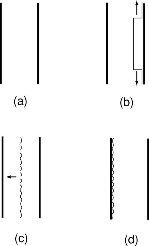
Figure 1: One possible set of initial conditions of the ekpyrotic scenario has the universe beginning in a cold, vacuous, nearly BPS state consisting of two static massive orbifold planes and a warped geometry in the intervening bulk (a) in which the curvature is low near the rightmost orbifold plane (the hidden brane) and high near the leftmost orbifold plane (the visible brane). Spontaneously, a bulk brane peels away from the hidden brane over some region of space (b), forming a terrace. The edges of the terrace expand outwards at light speed, while the interior moves very slowly towards the opposing visible brane. Although the bulk brane is flat on average, quantum fluctuations produce ripples over a wide range of length scales as the brane traverses the bulk (c). When the bulk brane collides with the visible brane, the ripples result in different regions colliding and reheating at slightly different times (d), thereby impressing a spectrum of density fluctuations on the visible universe. The energy from the collision is translated into matter and radiation, heating the universe to a temperature a few orders of magnitude smaller than the unification scale.

In our scenario, the collision sets the initial temperature and, consequently, the Hubble radius at the beginning of the FRW phase. The Hubble radius is generally infinitesimal compared to the collision region. Two events outside the Hubble radius are correlated since local conditions have a common causal link, namely, the collision with the bulk brane. Here we take advantage of the fact that the brane is a macroscopic, non-local object and exists for an indefinitely long period prior to the collision. That is, there is no direct connection between the time transpired preceding the collision or causality and the Hubble time. This feature provides a natural means for resolving the horizon problem.

As we have noted above, the boundary branes and the bulk brane are initially flat and parallel, as demanded by the BPS condition. Furthermore, the motion of the bulk brane along the fifth dimension maintains flatness (modulo small fluctuations around the flat background). Hence, the hot big bang universe resulting from the collision of a flat bulk brane with a flat visible brane is spatially flat. In other words, we address the flatness problem by beginning near a BPS ground state.

We do not require the initial state to be precisely BPS to resolve the horizon and flatness problems. It suffices if the universe is flat and homogeneous on scales ranging up to the (causal) particle horizon, as should occur naturally beginning from more general initial conditions. In the ekpyrotic scenario, the distance that particles can travel before collision is exponentially long because the bulk brane motion is extremely slow. As a result, the particle horizon at collision can be many more than 60 e-folds larger than the Hubble radius at collision (where the latter is determined by the radiation temperature at collision). That is, rather than introducing superluminal expansion to resolve the horizon and flatness problems, the ekpyrotic model relies on the assumption that the universe began in an empty, quasi-static BPS state which lasted an exponentially long time prior to the beginning of the hot big bang phase.

Quantum fluctuations introduce ripples in the bulk brane as it moves across the fifth dimension. During this motion there is a scale above which modes are frozen in, and below which they oscillate. This scale decreases with time in a manner akin to the Hubble radius of a collapsing Universe. The fluctuations span all scales up to this freeze-out scale, and we assume they begin in their quantum mechanical ground state. As the brane moves across the bulk, the effective Hubble radius shrinks by an exponential factor while the wavelengths of the modes decrease only logarithmically in time. Consequently, modes that begin inside the initial freeze-out scale end up exponentially far outside it, and exponentially far outside the final Hubble radius at the time of collision. The ripples in the bulk brane cause the collision between the bulk brane and the visible brane to occur at slightly different times in different regions of space. The time differences mean regions heat up and begin to cool at different times, resulting in adiabatic temperature and density fluctuations. Hence, as interpreted by an observer in the hot big bang FRW phase, the universe begins with a spectrum of density fluctuations that extend to exponentially large, super-horizon scales.

Of course, the spectrum of energy density perturbations must be nearly scale-invariant (Harrison-Zel’dovich [14]) to match observations of large-scale structure formation and temperature anisotropies in the cosmic microwave background. We find that this condition is satisfied if the potential attracting the bulk brane towards the visible brane is ultra weak at large separations. This is consistent with potentials generated by non-perturbative effects such as the exchange of virtual M2-branes (wrapped on holomorphic curves) between the bulk brane and either of the boundary branes.

While the spectrum of perturbations is approximately scale invariant, as with inflation there are small deviations from scale invariance. In the examples considered here, the spectrum is blue (the amplitude increases as the wavelength decreases), in contrast to typical inflationary models. With exponentially flat potentials, the spectrum is only marginally blue, consistent with current observations. On the other hand, the potential has no effect on the tensor (gravitational wave) perturbations, so the tensor spectrum is strongly blue (spectral index $n_{T}\approx 2$), in contrast to the slightly red ($n_{T}\leq 0$) spectrum predicted in most inflationary models. This prediction may be tested in near-future microwave background anisotropy and gravitational wave detector experiments.

For some aspects of the ekpyrotic scenario, such as the generation of quantum fluctuations, the description from the point-of-view of an observer on the bulk brane is the most intuitive. For that observer, the scale factor and Hubble radius appear to be shrinking because the warp factor decreases as the bulk brane moves across the fifth dimension. However, as observed from the near-stationary boundary orbifold planes, the universe is slowly expanding due to the gravitational backreaction caused by the bulk brane motion. Indeed, a feature of the scenario is that the bulk brane is responsible for initiating the expansion of the boundary branes. Furthermore, as we shall show, the brane gains kinetic energy due to its coupling to moduli fields. Upon impact, the bulk brane is absorbed by the visible brane in a so-called small-instanton phase transition (see Sec. II for details). This transition can change the gauge group on the visible brane. (For example, before collision the gauge group on the visible brane might be one of high symmetry, such as $E_{6}$, whereas after collision it becomes the standard model gauge group.) Furthermore, the number of light families of quarks and leptons on the visible brane may change during the transition. (For example, the visible brane might make a transition from having no light families of quarks and leptons to having three.) Upon collision, the kinetic energy gained by the bulk brane is converted to thermal excitations of the light degrees of freedom, and the hot big bang phase begins. Hence, the brane collision is not only responsible for initiating the expansion of the universe, but also for spontaneously breaking symmetries and for producing all of the quarks and leptons.

If the maximal temperature lies well below the mass scale of magnetic monopoles (and any other cosmologically dangerous massive, stable particles or defects), none will be generated during the collision and the monopole problem is avoided.

Although the ideas presented in this work may be applicable to more general brane-world scenarios, such as Randall-Sundrum, in developing our scenario we have felt that it is important to take as a guiding principle that any concepts introduced in this scenario be consistent with string theory and M-theory. By founding the model on concepts from heterotic M-theory, one knows from the outset that the theory is rich enough to contain the particles and symmetries necessary to explain the real universe and that nothing we introduce interferes with a fundamental theory of quantum gravity. We emphasize that our scenario does not rely on exponential warp factors (which are inconsistent with BPS ground states in heterotic M-theory) nor does it require large (millimeter-size) extra dimensions. For example, we consider here a bulk space whose size is only four or five orders of magnitude larger than the Planck length, consistent with Hořava-Witten phenomenology [15, 16]. All brane universe theories, including heterotic M-theory, suffer from some poorly understood aspects. For example, we have nothing to add here about the stability of the final, late time vacuum brane configuration. We will simply assume that branes in the early universe move under their respective forces until, after the big bang, some yet unknown physics stabilizes the vacuum.

Figure 1 summarizes the conceptual picture for one possible set of initial conditions. The remainder of this paper discusses our attempt to transform the conceptual framework into a concrete model. For this purpose, a number of technical advances have been required:

• an understanding of the perturbative BPS ground state (Section II) and how it can lead to the initial conditions desired for our scenario (Section III);

• a moduli space formulation of brane cosmology (Section IV A);

• a derivation of the equations of motion describing the propagation of bulk branes in a warped background in heterotic M-theory, including non-perturbative effects (Section IV B-D);

• a computation of the bulk brane-visible brane collision energy, which sets the initial temperature and expansion rate of the FRW phase (Section IV D);

• an analysis of how the gravitational backreaction due to the motion of the bulk brane induces the initial expansion of the universe (Section IV E);

• a computation of how ripples in the bulk brane translate into density perturbations after collision with the visible brane (Section V A);

• a theory of how quantum fluctuations produce a spectrum of ripples on the bulk brane as it propagates through a warped background (Section V B);

• a determination of the generic conditions for obtaining a nearly scale invariant spectrum and application of general principles to designing specific models (Section V B);

• a calculation of the tensor (gravitational wave) perturbation spectrum (Section V C);

• a recapitulation of the full scenario explaining how the different components rely on properties of moduli in 5d (Section VI A);

• a fully worked example which satisfies all cosmological constraints (Section VI A);

• and, a comparison of the ekpyrotic scenario with inflationary cosmology, especially differences in their predictions for the fluctuation spectrum (Section VI B).

In a subsequent paper, we shall elaborate on the moduli space formulation of brane cosmology and show how it leads to a novel resolution of the singularity problem of big bang cosmology [17].

The ekpyrotic proposal bears some relation to the pre-big bang scenario of Veneziano et al.[18, 19, 20] which begins with an almost empty but unstable vacuum state of string theory but which, then, undergoes superluminal deflation. Several important conceptual differences are discussed in Section VIB. Models with brane interactions that drive inflation followed by brane collision have also been considered.[21, 22, 23, 24, 25] Applications of the moduli space of M-theory and Hořava-Witten theory to cosmology have been explored previously in the context of inflation [26, 27, 28]. The distinguishing feature of the ekpyrotic model is that it avoids inflation or deflation altogether. A non-inflationary solution to the horizon problem was suggested in Ref. References, but it is not clear how to generate a nearly scale-invariant spectrum of density fluctuations without invoking inflation.

We hope that our technical advances may be useful in exploring other variants of this scenario. Some aspects remain more speculative, especially the theory of initial conditions (as one might expect) and non-perturbative contributions. A detailed understanding of these latter aspects awaits progress in heterotic M-theory.

II Terminology and Motivation from Heterotic M-theory

In this section, we briefly recount key features of heterotic M-theory that underlie and motivate the example of our ekpyrotic scenario given in this paper. Those who wish to understand the basic cosmological scenario without regard to the heterotic M-theory context can proceed directly to the next section.

Heterotic M-theory has its roots in the work of Hořava and Witten [5] who showed that compactifying (eleven-dimensional) M-theory on an $S_{1}/Z_{2}$ orbifold corresponds to the strong-coupling limit of heterotic $E_{8}\times E_{8}$ (ten-dimensional) string theory. Compactifying an additional six dimensions on a Calabi-Yau three-fold leads, in the low energy limit, to a four-dimensional ${\cal N}=1$ supersymmetric theory [15], the effective field theory that underlies many supersymmetric theories of particle phenomenology. By equating the effective gravitational and grand-unified coupling constants to their physical values, it was realized that the orbifold dimension is a few orders of magnitude larger than the characteristic size of the Calabi-Yau space [15, 16]. There is, therefore, a substantial energy range over which the universe is effectively five-dimensional, being bounded in the fifth-dimension by two $(3+1)$-dimensional “end-of-the-world” $S^{1}/Z_{2}$ orbifold fixed planes. By compactifying Hořava-Witten theory on a Calabi-Yau three-fold, in the presence of a non-vanishing $G$-flux background (that is, a non-zero field strength of the three-form of eleven dimensional M-theory) required by anomaly cancellation, the authors of Refs. References and References were able to derive the explicit effective action describing this five-dimensional regime. This action is a specific gauged version of ${\cal N}=1$ supergravity in five dimensions and includes “cosmological” potential terms that always arise in the gauged context. It was shown in Ref. References that these potentials support BPS 3-brane solutions of the equations of motion, the minimal vacuum consisting of two 3-branes, each coinciding with one of the $S_{1}/Z_{2}$ orbifold fixed planes. These boundary 3-branes (the visible brane and the hidden brane) each inherit a (spontaneously broken) ${\cal N}=1$ $E_{8}$ super gauge multiplet from Hořava-Witten theory. This five-dimensional effective theory with BPS 3-brane vacua is called heterotic M-theory. It is a fundamental paradigm for “brane universe” scenarios of particle physics.

In order to support a realistic theory, heterotic M-theory must include sufficient gauge symmetry and particle content on the 3-brane boundaries. In the compactification discussed above, the authors of Refs. References and References initially made use of the standard embedding of the spin connection into the gauge connection, leading to an $E_{6}$ gauge theory on the visible 3-brane while the gauge theory on the hidden 3-brane is $E_{8}$. Subsequently, more general embeddings than the standard one were considered [31]. Generically, such non-standard embeddings (topologically non-trivial configurations of gauge fields known as $G$-instantons) induce different gauge groups on the orbifold fixed planes. For example, it was shown in Refs. References and References that one can obtain grand unified gauge groups such as $SO(10)$, $SU(5)$ and the standard model gauge group $SU(3)_{C}\times SU(2)_{L}\times U(1)_{Y}$ on the visible brane by appropriate choice of $G$-instanton. Similarly, one can obtain smaller gauge groups on the hidden brane, such as $E_{7}$ and $E_{6}$. However, as demonstrated in Refs. References-References, requiring a physically interesting gauge group such as $SU(3)_{C}\times SU(2)_{L}\times U(1)_{Y}$, along with the requirement that there be three families of quarks and leptons, typically leads to the constraint that there must be a certain number of M5-branes in the bulk space in order to make the theory anomaly-free. These M5-branes are wrapped on holomorphic curves in the Calabi-Yau manifold, and appear as 3-branes in the five-dimensional effective theory. The five-dimensional effective action for non-standard embeddings and bulk space M5-branes was derived in Ref. References. The key conclusion from this body of work is that heterotic M-theory can incorporate the particle content and symmetries required for a realistic low-energy effective theory of particle phenomenology. There has been a considerable amount of literature studying both the four-dimensional limit of Hořava-Witten theory [34] and heterotic M-theory [35].

A feature of M5-branes which we will utilize is that they are allowed to move along the orbifold direction. It is important to note that the M5-brane motion through the bulk is not “free” motion. Rather, non-perturbative effects, such as the exchange of virtual open supermembranes stretched between a boundary brane and the bulk M5-brane, can produce a force between them. The corresponding potential energy can, in principle, be computed from M-theory. Explicit calculations of the supermembrane-induced superpotentials in the effective four-dimensional theory have been carried out in Refs. References and References. Combined with the M5-brane contribution to the Kähler potential presented in Ref. References, one can obtain an expression for the supermembrane contribution to the M5-brane potential energy. These non-perturbative effects cause the bulk brane to move along the extra dimension. In particular, it may come into contact with one of the orbifold fixed planes. In this case, the branes undergo a “small instanton” phase transition which effectively dissolves the M5-brane, absorbing its “data” into the $G$-instanton [39]. Such a phase transition at the visible brane may change the number of families of quarks and leptons as well as the gauge group. For instance, the observable 3-brane may go from having no light families of quarks and leptons prior to collision to having three families after the phase transition.

It is in this five-dimensional world of heterotic M-theory, bounded at the ends of the fifth dimension by our visible world and a hidden world, and supporting moving five-branes subject to catastrophic family and gauge changing collisions with our visible 3-brane, that we propose to find a new theory of the very early universe.

III Initial conditions

All cosmological models, including the hot big bang and the inflationary scenario, rest on assumptions about the initial conditions. Despite attempts, no rigorous theory of initial conditions yet exists.

Inflationary theory conventionally assumes that the universe emerges in a high energy state of no particular symmetry that is rapidly expanding. If traced backward in time, such states possess an initial singularity. This is only one of several fundamental obstacles to constructing a well-defined theory of ‘generic’ inflationary initial conditions. For a theory based on such general and uncertain initial conditions, it is essential that there be a dynamical attractor mechanism that makes the universe more homogeneous as expansion proceeds, since such a mechanism provides hope that the uncertainty associated with the initial conditions is, in the end, irrelevant. Superluminal expansion provides that mechanism.

The ekpyrotic model is instead built on the assumption that the initial state is quasi-static, nearly vacuous and long-lived, with properties dictated by symmetry. So, by construction, the initial state is special, both physically and mathematically. In this case, while a dynamical attractor mechanism may be possible (see below), it is not essential. One can envisage the possibility that the initial conditions are simply the result of a selection rule dictating maximal symmetry and nearly zero energy.

Within the context of superstring theory and M-theory, a natural choice with the above properties is the BPS (Bogolmon’yi-Prasad-Sommerfeld) state.[6] The BPS property is already required from particle physics in order to have a low-energy, four-dimensional effective action with ${\cal N}=1$ supersymmetry, necessary for a realistic phenomenology. For our purposes, the BPS state is ideal because, not only is it homogeneous, as one might suppose, but it is also flat. That is, the BPS condition links curvature and homogeneity. It requires the two boundary branes to be parallel.

The BPS condition also requires the bulk brane to be nearly stationary. If the bulk brane has a small initial velocity, it is free to move along the fifth dimension. Assuming the bulk brane to be much lighter than the bounding branes enables us to treat its backreaction as a small perturbation on the geometry. Non-perturbative effects can modify this picture by introducing a potential for the bulk brane. For example, a bounding brane and bulk brane can interact by the exchange of M2-branes wrapped on holomorphic curves, resulting in a potential drawing the bulk brane towards our visible brane. In Section V, we shall see that the non-perturbative potential plays an important role in determining the spectrum of energy density fluctuations following the collision of the bulk brane with our visible brane.

We do not rule out the possibility of a dynamical attractor mechanism that drives the universe towards the BPS state beginning from some more general initial condition. Such parallelism would be a natural consequence of all the branes emerging from one parent brane. Another appealing possibility is to begin with a configuration consisting of only the two bounding 3-branes. The configuration may have some curvature and ripples, but these can be dissipated by radiating excitations tangential to the branes and having them travel off to infinity. Then, at some instant, the hidden brane may under go a “small instanton” transition which causes a bulk brane to peel off. While little is known about the dynamics of this peeling off, it is reasonable to imagine a process similar to bubble nucleation in first order phase transitions. We suppose that there is a long-range, attractive, non-perturbative potential that draws the bulk brane towards our visible brane, as shown in Figure 2. Very close to the hidden brane, there may be a short-range attractive force between the bulk brane and the hidden brane due to small-instanton physics (not shown in the Figure). The situation is similar to false vacuum decay where the position of the bulk brane along the fifth dimension, $Y$, plays the role of the order parameter or scalar field. Classically, a bulk brane attached to the hidden brane is kept there by the energy barrier. However, quantum mechanically, it is possible to nucleate a patch of brane for which $Y$ lies on the other side of the energy barrier. At the edges of the patch, the brane stretches back towards and joins onto the orbifold plane. The nucleated patch would correspond to the minimum action tunneling configuration. We conjecture that, as in the case of bubble nucleation, the configuration would be one with maximal symmetry. In this case, this configuration would correspond to a patch at fixed $Y$ with a spherical boundary along the transverse dimensions. The nucleation would appear as the spontaneous appearance of a brane that forms a flat, spherical terrace at fixed $Y$ parallel to the bounding branes (i.e., flat). Once nucleated, the boundaries of the terrace would spread outwards at the speed of light, analogous to the outward expansion of a bubble wall in false vacuum decay. At the same time, the brane (the terrace) would travel towards the visible brane due to the non-perturbative potential. As we shall see in Section IV, this motion is very slow (logarithmic with time) so that the nucleation rate is essentially instantaneous compared with the time scale of transverse motion. In other words, for our purposes, the nucleation process corresponds to a nearly infinite brane peeling off almost instantaneously.

Beginning in an empty, quasi-static state addresses the horizon and flatness problems, but one should not underestimate the remaining challenges: how to generate a hot universe, and how to generate perturbations required for large-scale structure. The remarkable feature of the ekpyrotic picture, as shown in the forthcoming sections, is that brane collision naturally serves both roles.

Figure 2: Sketch of the exponential potential $V(Y)=-ve^{-m\alpha Y}$ (the line of zero potential energy corresponds to the dotted line). The potential attracts the bulk brane towards the visible brane. The force is strongest near the visible brane and tends to zero at large distances.

In either setup, we begin with a flat bulk brane, either a finite patch or an infinite plane, which starts nearly at rest, and a non-perturbative force drawing it towards the visible brane. These initial conditions are sufficient to enable our scenario.

IV Propagation of the Bulk Brane

IV.1 Moduli Space Actions for Brane-World Gravity

In this section, we discuss the moduli space approximation which we shall employ throughout our analysis. This approximation may be used when there is a continuous family of static solutions of the field equations, of degenerate action. It is the basis for much of what is known of the classical and quantum properties of solitons such as magnetic monopoles and vortices [40]. It is also a powerful tool for cosmology as it neatly approximates the five dimensional theory in the regime where the rate of change of the geometry, as measured, for example, by the four dimensional Hubble constant $H$ is smaller than the typical spatial curvature scale in the static solutions. The moduli are the parameters specifying the family of static solutions, ‘flat directions’ in configuration space along which slow dynamical evolution is possible. During such evolution the excitation in other directions is consistently small provided those directions are stable and characterized by large oscillatory frequencies.

The action on moduli space is obtained by substituting the static solutions into the full action with the modular parameters represented as space-time dependent moduli fields, $Q^{I}$, where $I$ runs over all the moduli fields. If we consider the time dependence first, as we shall do for the homogeneous background solutions, the moduli space action takes the form

$${\cal S}=\int d\tau\,G_{IJ}(Q)\dot{Q^{I}}\dot{Q^{J}}$$ (1)

where $G_{IJ}(Q)$ is a matrix-valued function of the moduli fields. This is the action for a non-relativistic particle moving in a background metric $G_{IJ}(Q)$, the metric on moduli space. For truly degenerate static solutions, the potential term must be constant, and therefore irrelevant to the dynamics. Even if a weak potential $V$ is additionally present, as it shall be in our discussion below, the moduli approximation is still valid as long as the dynamical evolution consists in the first approximation of an adiabatic progression through the space of static solutions.

In the next section we compute the moduli space action for heterotic M-theory. First, however, it is instructive to consider a simpler model which demonstrates similar physical effects and is of some interest in its own right. This model, discussed by Randall and Sundrum [10], consists of a five dimensional bulk described by Einstein gravity with a negative cosmological constant $\Lambda$, bounded by a pair of branes with tension $\pm\alpha$. The brane tension must be fine tuned to the value $\alpha=(3|\Lambda|/(4\pi G_{5}))^{1/2}$ in order for static solutions to exist. Because there are few moduli, the model is simple to analyze and illustrative of some important effects. However, as we emphasize below, there are reasons for taking heterotic M-theory more seriously as a candidate fundamental description.

In the Randall-Sundrum model, the static field equations allow a two-parameter family of solutions, with metric

$$ds^{2}=-n^{2}d\tau^{2}+a^{2}d\vec{x}^{2}+dy^{2},\quad a=e^{{y/L}},\quad n=Na,\qquad y_{1}\leq y\leq y_{0},$$ (2)

and the positive (negative) tension branes located at $y_{0}$ ($y_{1}$) respectively. $L$ is the Anti-de Sitter (AdS) radius given by $L^{2}=3/(4\pi G_{5}|\Lambda|)$, and $N$ is an arbitrary constant.

The above solutions are specified by the three moduli $N$, $y_{0}$ and $y_{1}$. We now allow them to be time dependent. The lapse function $N(t)$ is associated with time reparametrization invariance and, hence, not a physical degree of freedom. The other two moduli represent the proper distance between the branes, but also the time-dependent cosmological ‘scale factors’ $a_{0}=e^{y_{0}/L}$ and $a_{1}=e^{y_{1}/L}$ on each brane. We shall see in a moment how these combine to give four-dimensional gravity with a massless scalar, related to the proper separation between the branes.

To compute the moduli space action it is convenient to change from the coordinates in Eq. (2) to coordinates in which the branes are fixed. This is accomplished by setting $y=(y_{0}-y_{1})\tilde{y}+y_{1}$, and the branes are now located at $\tilde{y}=0$ and 1 respectively. We substitute the ansatz Eq. (2) into the five dimensional action and integrate over $\tilde{y}$. All potential terms cancel. Since the branes do not move in the $\tilde{y}$ coordinates, the kinetic terms arise only from the five dimensional Ricci scalar, which yields the result

$${\cal S}={L\over 16\pi G_{5}}\int d\tau d^{3}xN^{-1}\,6(\dot{a}_{1}^{2}-\dot{a}_{0}^{2}).$$ (3)

Thus the metric on moduli space is just the 1+1 Minkowski metric, and we infer that moduli space in this theory is completely flat.

We may now change coordinates to

$$a_{0}=a\,\cosh f\qquad a_{1}=a\,\sinh f$$ (4)

where $a^{2}=a_{0}^{2}-a_{1}^{2}$, and the proper separation between the branes is just $L\ln(a_{0}/a_{1})=L\ln(\coth f)$. The action (3) then becomes

$${\cal S}={1\over 16\pi G_{4}}\int d\tau d^{3}xN^{-1}\,6\left(-\dot{a}^{2}+a^{2}\dot{f}^{2}\right),$$ (5)

where $G_{4}=G_{5}L^{-1}$, just the action for four dimensional gravity coupled to a massless scalar field $f$. This is the ‘radion’ field [41]. Note that the ‘4d Einstein frame scale factor’ $a$ is not the scale factor that is seen by matter localized on the branes: such matter sees $a_{0}$ or $a_{1}$. As we shall see, it is perfectly possible for both of the latter scale factors to expand while $a$ contracts.

The general solution to the moduli space theory is easily obtained from (3): the scale factors evolve linearly in conformal time $\tau$, with $\dot{a}_{1}=\pm\dot{a}_{0}$. From the point of view of each brane, the motion of the other brane acts as a density of radiation (i.e., allowing $\dot{a}_{1,0}=$ constant). Although the moduli space theory has identical local equations to four-dimensional gravity coupled to a massless scalar, the geometrical interpretation is very different, so that what is singular from one point of view may be non-singular from the other [17].

To obtain an action that might describe the present, hot big bang phase with fixed gravitational constant, one might add a potential $V(f)$ which fixes the interbrane separation $f$, causing it to no longer be a free modulus (e.g., see Ref. References). Likewise adding extra fields on either brane, one sees that a standard Friedmann constraint is obtained from the variation with respect to $N$. Generally the matter couplings will involve the field $f$. However, if $V(f)$ rises steeply away from its minimum and if its value at the minimum is zero (so that there is no vacuum energy contribution), $f$ will not evolve appreciably and four dimensional gravity will be accurately reproduced.

We imagine that, prior to the big bang phase, there is an additional, positive tension bulk brane. For static solutions to occur, we require that the three brane tensions sum to zero. Positivity of the bulk brane tension imposes that the cosmological constant to its right, $\Lambda_{0}$, be smaller in magnitude than that to its left, $\Lambda_{1}$, so that the corresponding AdS radii obey $L_{0}>L_{1}$.

For the three brane case we obtain the moduli space action

$${\cal S}={1\over 16\pi G_{5}}\int d\tau d^{3}xN^{-1}6\left(-L_{0}\dot{a}_{0}^{2}+(L_{0}-L_{1})\dot{a}_{B}^{2}+L_{1}\dot{a}_{1}^{2}\right),$$ (6)

where $a_{B}$ is the scale factor on the bulk brane. Again this is remarkably simple, just Minkowski space of 2+1 dimensions. Likewise for $N$ parallel branes, all with positive tension except the negative tension boundary brane, the system possesses a metric which is that for $N$-dimensional Minkowski space. Note that the ‘masses’ appearing in the kinetic terms for the boundary branes are the opposite of what one might naively expect. Namely, the positive tension boundary brane (hidden brane) has the negative ‘mass’ $-L_{0}$, whereas the negative tension boundary brane (visible brane) has a positive ‘mass’ $L_{1}$. The magnitudes of these terms are also surprising: the visible brane has the greater magnitude tension, but the smaller magnitude moduli space mass.

Just as for the brane-antibrane system, when more branes are present one can change variables to those in which the theory resembles four dimensional Einstein gravity coupled to massless fields. For three branes, the required change of variables is

$$a_{0} = a\,{\rm cosh}f,$$ (7)

$$a_{B} = (L_{0}/(L_{0}-L_{1}))^{{1\over 2}}\,a\,{\rm sinh}f\,{\rm cos}\theta,$$ (8)

$$a_{1} = (L_{0}/L_{1})^{{1\over 2}}\,a\,{\rm sinh}f\,{\rm sin}\theta,$$ (9)

and the scalar field kinetic term takes the form $a^{2}(\dot{f}^{2}+\dot{\theta}^{2}\sinh^{2}f)$. The scalar fields live on the hyperbolic plane $H^{2}$, and there is a nontrivial Kähler potential. When we introduce potentials, we must do so in a manner which respects four dimensional general coordinate invariance. This restricts the form to

$$\Delta{\cal S}=-\int d\tau d^{3}xNa^{4}V(f,\theta).$$ (10)

We shall assume that the system starts out nearly static, and that the potential energy is always negative, so that we are clearly not using inflation to drive expansion. We further assume that the interaction potential draws the bulk brane away from the hidden brane towards the visible brane. The original variables in Eq. (6) provide some insight into what happens. We consider an interaction between $a_{0}$ and $a_{B}$ causing the latter to decrease. But since $a_{0}$ has a negative ‘mass’ it is actually pushed in the same direction and thus contracts. Similarly an interaction potential between $a_{0}$ and $a_{1}$ can have the opposite effect: causing both $a_{0}$ and $a_{1}$ to expand. Figure (3) shows an example, with the bulk brane being pushed across the gap, and the visible brane being attracted towards it. The hidden brane actually ‘bounces’ (this is barely visible in the Figure) due to a competition between the two effects, so that by the collision between bulk and visible branes, both outer boundary branes are actually expanding; that is, $a_{0}$ and $a_{1}$ are both increasing. At first sight this appears inconsistent with the four dimensional point of view: if the system starts out static, and with all potentials negative, then the 4d Einstein frame scale factor $a$ must contract throughout. The two points of view are consistent because $\dot{a}_{1}$ contributes negatively to $\dot{a}$. Since $a_{1}$ is expanding rapidly compared to $a_{0}$, $a$ is indeed contracting, as shown in the Figure. Of course what is happening physically is that the fifth dimension is collapsing, a well known hazard of Kaluza-Klein cosmology. Here, the inter-brane separation is decreasing while the scale factors seen by matter on the branes are expanding.

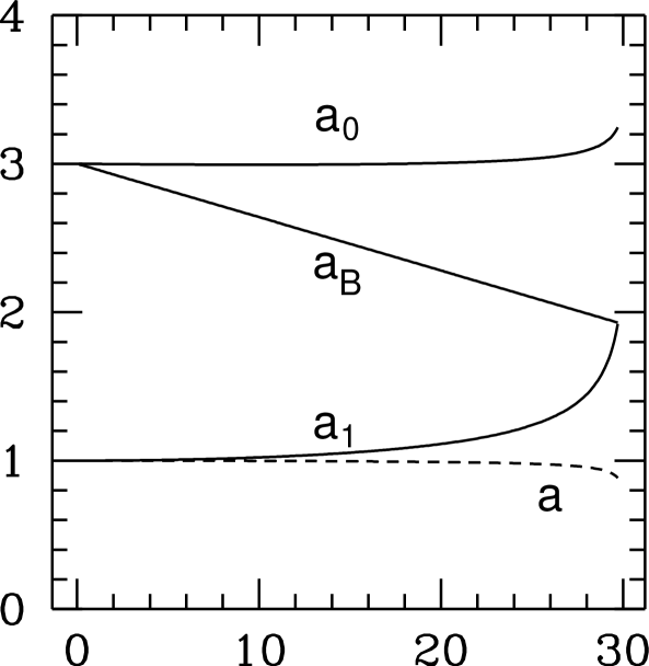
Figure 3: Evolution of scale factors in a three-brane system where a bulk brane is drawn across from the hidden brane to the visible brane. The solid lines show (from top to bottom) the scale factors on the hidden brane ($a_{0}$), the bulk brane ($a_{B}$) and the visible brane ($a_{1}$). At collision between the bulk brane and the visible brane, both boundary branes are expanding. The evolution of the 4d Einstein frame scale factor $a$ is also shown as a dashed line: it contracts throughout.

What happens when the bulk brane meets the boundary? A matching condition is needed to determine the resulting cosmology. The initial state is specified by the scale factors $a_{0}$, $a_{B}$ and $a_{1}$ and their time derivatives, the final state by $a_{0}$, $a_{1}$ and their time derivatives, plus the coordinates and momenta of any excitations produced in the collision.

One expects that the scale factors $a$, $a_{1}$ and $a_{0}$ should be continuous: likewise $\dot{a}_{0}$ would be expected to be continuous if no bulk brane hits the hidden brane, and if no constraint on the size of the extra dimension is imposed. However, $\dot{a}_{1}$ cannot be continuous since the bulk brane imparts some momentum on the visible brane. The momentum conservation condition can be expressed as

$$L_{0}a^{i}_{0}\dot{a}_{0}^{i}-(L_{0}-L_{1})\dot{a}_{B}^{i}a_{B}^{i}-L_{1}\dot{a}_{1}^{i}a_{1}^{i}=L_{0}a_{0}^{f}\dot{a}_{0}^{f}-L_{0}a_{1}^{f}\dot{a}_{1}^{f},$$ (11)

where $i$ and $f$ subscripts label initial and final quantities. Conservation of momentum applies if the forces derive from a potential $V$ which is short-ranged and translation invariant and if there is no other entity that carries momentum after collision. The above conditions imply the continuity of the ‘4d Einstein frame scale factor’ $a$ and its time derivative.

This matching condition, if correct, would pose a serious problem for our scenario since it implies that the four dimensional scale factor $a$ is contracting after collision, at the beginning of the hot big bang phase. Specifically, the matching condition suggests a simple continuation of the motion in Figure 3 after collision in which both branes are expanding but $a$ is decreasing because the two branes are approaching one another and the fifth dimension is collapsing.

In the M-theory models which we consider in this paper, we shall simply impose a constraint on moduli space which ensures that the distance between the visible and hidden branes becomes fixed after collision, as required to converge to the Hořava-Witten picture. The constraint corresponds to fixing $a_{0}/a_{1}$ after collision, forcing a discontinuity in both $\dot{a}_{1}$ and $\dot{a}_{0}$. In this case the momentum matching condition (continuity of $\dot{a}$) yields rather paradoxical behavior in which both $\dot{a}_{1}$ and $\dot{a}_{0}$ reverse after collision, so the universe collapses. This does not seem physically plausible, especially when matter is produced at collision, and the expansion of the matter would then have to be reversed as the size of the fifth dimension became fixed. More plausible is that $\dot{a}$ is also discontinuous: the branes collide, their separation becomes fixed, and the pair continue in the same direction of motion (expansion) as before collision. Here we simply wish to flag this issue as one that we have not resolved in the M-theory models considered here: more work is needed to do so.

We have identified at least one mechanism for avoiding contraction or collision while still remaining within the moduli space approximation. We have constructed models for branes in AdS employing ‘non-minimal’ corrections to the kinetic terms of $a_{1,0}$, which are allowed by four dimensional general coordinate invariance. These non-minimal kinetic terms both stabilize the size of the extra dimension and allow final expansion from static initial conditions, with negative potentials.[17]

Another possibility is that the moduli space approximation break-down at collision (it must break down, since radiation is produced) leads to the release of radiation into the bulk. This is prohibited by planar symmetry in the AdS example, but is possible in the more general M-theory context. Radiation emitted into the bulk contributes to the pressure $T_{55}$, which, from the $G_{55}$ Einstein equations, acts to decelerate $a_{1}$. The emitted radiation is redshifted as it crosses the bulk, so is likely to have less effect on the hidden brane if it is absorbed there. The net result would be a slowing of $a_{1}$, causing the effective scale factor $a$ to increase.

We do not want to understate the challenge of obtaining a final expanding universe with stabilized fifth dimension. In a conventional four-dimensional theory (Einstein gravity plus scalar fields) it would simply be impossible to start from zero energy and, through evolution involving negative potentials, obtain a final expanding universe. Our point is that brane world scenarios offer ways around this ‘no-go theorem’, which we have just begun to explore.

The AdS examples we have discussed are instructive in that they are easier to analyze than the full M-theory case. However, as mentioned above, it is unlikely that these model theories are quantum mechanically consistent. The most obvious problem is that fine tuning is needed to balance the brane tension against the cosmological term. Without this balance, no static solutions are possible. Computing the quantum corrections may in fact be impossible since, in the thin-brane limit, these are generally infinite and non-renormalizable.

Therefore, for the remainder of the paper, we turn to analogous examples in heterotic M-theory, which is more complex but has other advantages. The branes in this theory are BPS states, protected from quantum corrections by supersymmetry. Their tensions are fixed by exact quantum mechanical symmetries and there is no fine tuning problem analogous to that present in the Randall-Sundrum models.

IV.2 The Background BPS Solution in Heterotic M-theory

The five-dimensional effective action of heterotic M-theory was derived in Refs. References and References. Its field content includes a myriad of moduli, most of which will be assumed frozen in this paper. We shall, therefore, use a simplified action describing gravity $g_{\gamma\delta}$, the universal “breathing” modulus of the Calabi-Yau three-fold $\phi$, a four-form gauge field ${\cal A}_{\gamma\delta\epsilon\zeta}$ with field strength ${\cal F}=d{\cal A}$ and a single bulk M5-brane. It is given by

$$S=\frac{M_{5}^{3}}{2}\int_{{\cal M}_{5}}d^{5}x\sqrt{-g}\left({\cal R}-\frac{1}{2}(\partial\phi)^{2}-\frac{3}{2}\frac{e^{2\phi}{\cal F}^{2}}{5!}\right)$$

$$\;\;\;\;\;\;-3\sum_{i=1}^{3}\alpha_{i}M_{5}^{3}\int_{{\cal M}_{4}^{(i)}}d^{4}\xi_{(i)}\left(\sqrt{-h_{(i)}}e^{-\phi}-\frac{\epsilon^{\mu\nu\kappa\lambda}}{4!}{\cal A}_{\gamma\delta\epsilon\zeta}\partial_{\mu}X^{\gamma}_{(i)}\partial_{\nu}X^{\delta}_{(i)}\partial_{\kappa}X^{\epsilon}_{(i)}\partial_{\lambda}X^{\zeta}_{(i)}\right),$$ (12)

where $\gamma,\delta,\epsilon,\zeta=0,\dots,4$, $\mu,\nu,\dots=0,\dots,3$. The space-time is a five-dimensional manifold ${\cal M}_{5}$ with coordinates $x^{\gamma}$. The four-dimensional manifolds ${\cal M}_{4}^{(i)}$, $i=1,2,3$ are the visible, hidden, and bulk branes respectively, and have internal coordinates $\xi^{\mu}_{(i)}$ and tension $\alpha_{i}M_{5}^{3}$. Note that $\alpha_{i}$ has dimension of mass. If we denote $\alpha_{1}\equiv-\alpha$, $\alpha_{2}\equiv\alpha-\beta$, and $\alpha_{3}\equiv\beta$, then the visible brane has tension $-\alpha M_{5}^{3}$, the hidden brane $(\alpha-\beta)M_{5}^{3}$, and the bulk brane $\beta M_{5}^{3}$. It is straightforward to show that the tension of the bulk brane, $\beta M_{5}^{3}$, must always be positive. Furthermore, one can easily deduce that the tension on the visible brane, $-\alpha M_{5}^{3}$, can be either positive or negative. The ekpyrotic scenario can be applied, in principle, to any such vacua. In this paper, for specificity, we will always take $\alpha>0$, so that the tension on the visible brane is negative. Furthermore, we will choose $\beta$ such that $\alpha-\beta>0$, that is, the tension of the hidden brane is positive. The tensor $h^{(i)}_{\mu\nu}$ is the induced metric (and $h_{(i)}$ its determinant) on ${\cal M}_{4}^{(i)}$. The functions $X^{\gamma}_{(i)}(\xi_{(i)}^{\mu})$ are the coordinates in ${\cal M}_{5}$ of a point on ${\cal M}_{4}^{(i)}$ with coordinates $\xi_{(i)}^{\mu}$. In other words, $X^{\gamma}_{(i)}(\xi_{(i)}^{\mu})$ describe the embedding of the branes into ${\cal M}_{5}$.

The BPS solution of Lukas, Ovrut, and Waldram [6] is then given by

$$ds^{2}=D(y)(-N^{2}d\tau^{2}+A^{2}d\vec{x}^{2})+B^{2}D^{4}(y)dy^{2}$$

$$e^{\phi}=BD^{3}(y)$$

$${\cal F}_{0123Y}=-\alpha A^{3}NB^{-1}D^{-2}(y)\;\;\;\;\;\;\;\;\;\;\;\;\;{\rm for}\;\;y<Y$$

$$\;\;\;\;\;\;\;\;\;\;\;\;=-(\alpha-\beta)A^{3}NB^{-1}D^{-2}(y)\;\;\;\;{\rm for}\;\;y>Y,$$ (13)

where

$$D(y)=\alpha y+C\;\;\;\;\;\;\;\;\;\;\;\;\;\;\;\;\;\;\;\;\;\;\;\;\;\;{\rm for}\;\;y<Y$$

$$\;\;\;\;\;\;\;\;\;=(\alpha-\beta)y+C+\beta Y\;\;\;\;\;\;\;{\rm for}\;\;y>Y,$$ (14)

and $A,B,C,N$ and $Y$ are constants. Note that $A,B,C,N$ are dimensionless and $Y$ has the dimension of length. The visible and hidden boundary branes are located at $y=0$ and $y=R$, respectively, and the bulk brane is located at $y=Y$, $0\leq Y\leq R$. We assume that $C>0$ so that the curvature singularity at $D=0$ does not fall between the boundary branes. Note that $y=0$ lies in the region of smaller volume while $y=R$ lies in the region of larger volume.

Finally, note that inserting the solution of the four-form equation of motion into Eq. (12) yields precisely the bulk action given in Ref. References with charge $-\alpha$ in the interval $0\leq y\leq Y$ and charge $-\alpha+\beta$ in the interval $Y\leq y\leq R$. The formulation of the action Eq. (12) using the four-form ${\cal{A}}$ is particularly useful when the theory contains bulk branes, as is the case in ekpyrotic theory.

IV.3 The Moduli Space Action of Heterotic M-theory

As in Section IV.1, we shall use the moduli space approximation to study the dynamics of heterotic M-theory with a bulk brane. The static BPS solution involves five constants $A,B,C,N$, and $Y$. These now become the moduli fields, $Q^{I}=(A(\vec{x},\tau),B(\vec{x},\tau),\,C(\vec{x},\tau),\,N(\vec{x},\tau),\,Y(\vec{x},\tau))$. In the limit of homogeneity and isotropy, the moduli fields are functions of time only. Substituting the static ansatz (13) into the action (12), and integrating over $y$, we obtain the moduli space action ${\cal S}_{mod}$ with Lagrangian density

$${\cal L}_{mod}=G_{IJ}(Q)\dot{Q}^{I}\dot{Q}^{J}-V(Q)={\cal L}_{bulk}+{\cal L}_{\beta},$$ (15)

where

$${\cal L}_{bulk}=-\frac{3A^{3}BI_{3}M_{5}^{3}}{N}\left\{\left(\frac{\dot{A}}{A}\right)^{2}+\left(\frac{\dot{A}}{A}\right)\left[\left(\frac{\dot{B}}{B}\right)+\frac{3I_{2}}{I_{3}}\dot{C}+\frac{3I_{2b}}{I_{3}}\beta\dot{Y}\right]\right\}$$

$$\;\;\;\;\;\;\;\;\;\;\;\;-\frac{3A^{3}BI_{3}M_{5}^{3}}{N}\left\{-\frac{1}{12}\left(\frac{\dot{B}}{B}\right)^{2}+\frac{I_{1}}{2I_{3}}\dot{C}^{2}+\frac{I_{1b}}{I_{3}}\dot{C}\beta\dot{Y}+\frac{I_{1b}}{2I_{3}}\beta^{2}\dot{Y}^{2}\right\}$$

$${\cal L}_{\beta}=\frac{3\beta M_{5}^{3}A^{3}B}{N}\left[\frac{1}{2}D^{2}(Y)\dot{Y}^{2}-N^{2}V(Y)\right]$$ (16)

and

$$I_{ma}\equiv 2\int_{0}^{Y}D^{m}dy=\frac{2}{\alpha(m+1)}[(\alpha Y+C)^{m+1}-C^{m+1}]$$

$$I_{mb}\equiv 2\int_{Y}^{R}D^{m}dy=\frac{2}{(\alpha-\beta)(m+1)}[((\alpha-\beta)R+C+\beta Y)^{m+1}-(\alpha Y+C)^{m+1}]$$

$$I_{m}\equiv I_{ma}+I_{mb}.$$ (17)

Note that $I_{m}$ has the dimension of length. We see from Eq. (16) that the Lagrangian of the 4d effective theory is the sum of two parts, ${\cal L}_{bulk}$ and ${\cal L}_{\beta}$. The first contribution, ${\cal L}_{bulk}$, comes from the bulk part of the five-dimensional action, whereas the second contribution, ${\cal L}_{\beta}$, is the Lagrangian of the bulk brane. Note that we have added by hand a potential $V(Y)$ in ${\cal L}_{\beta}$ which is meant to describe non-perturbative interactions between the bulk brane and the boundary branes[36, 37, 38]. The actions of the two boundary branes, which are at fixed values of $y$, do not contribute to the 4d effective action. Their contribution is canceled by bulk terms upon integration over $y$. This cancellation is crucial, since it yields a 4d effective theory with no potentials for $A,B,C$, or $N$, thereby confirming that these fields are truly moduli of the theory.

Eq. (16) is analogous to the action for gravity with scale factor $A$ coupled to scalar fields. Since the overall factor of $BI_{3}M_{5}^{3}$ will generically be time-dependent before collision, it follows that the scalar fields $B,C$, and $Y$ are non-minimally coupled to gravity. In order to match onto a theory with fixed Newton’s constant $G_{4}$, we shall impose the condition that this factor become constant after collision. Hence, after collision, we can identify the 4d effective Planck mass as

$$M_{pl}^{2}=\frac{BM_{5}^{2}(I_{3}M_{5})}{\alpha R+C}$$ (18)

where $I_{3}$ is evaluated at $Y=0$ and for $B,C$ at the moment of collision. Note that in the limit $(\alpha-\beta)R\ll C$, this expression agrees with the 4d Planck mass identified in Ref. References.

At this point, one can define a new scale factor $a\equiv A(BI_{3}M_{5})^{1/2}$, as well as $n\equiv N(BI_{3}M_{5})^{1/2}$. This has the effect of removing off-diagonal terms in the moduli space metric that couple the field $A$ to the other variables. In these new variables, the bulk Lagrangian becomes

$${\cal L}_{bulk}=\frac{3a^{3}M_{5}^{2}}{n}\left\{-\left(\frac{\dot{a}}{a}\right)^{2}+\frac{1}{3}\left(\frac{\dot{B}}{B}\right)^{2}+\frac{1}{2}\frac{\dot{B}}{B}\frac{\dot{I}_{3}}{I_{3}}\right\}$$

$$\;\;\;\;\;\;\;\;\;\;+\frac{3a^{3}M_{5}^{2}}{n}\left\{\left(\frac{9I_{2}^{2}}{4I_{3}^{2}}-\frac{I_{1}}{2I_{3}}\right)\dot{C}^{2}+\left(\frac{9I_{2}I_{2b}}{2I_{3}^{2}}-\frac{I_{1b}}{I_{3}}\right)\dot{C}\beta\dot{Y}+\left(\frac{9I_{2b}^{2}}{4I_{3}^{2}}-\frac{I_{1b}}{2I_{3}}\right)\beta^{2}\dot{Y}^{2}\right\}.$$ (19)

In this form, it is clear that $a$ is an scale factor analogous to the variable $a$ of the previous section. The moduli $B$, $C$ and $Y$ behave effectively as scalar fields, albeit with nontrivial kinetic terms.

In analogy with the example in Section IV A and the discussion following Eq. (5), we now impose two constraints consistent with four dimensional covariance. These reduce the moduli degrees of freedom and simplify the system. Namely, we shall impose that

$$B=constant$$

$$C=constant.$$ (20)

At the moment of collision, the modulus $Y$ disappears from the theory. The above conditions then imply that the distance between the boundary branes as well as the volume of the Calabi-Yau three-fold become fixed. This is necessary if we want to match onto a theory with fixed gravitational and gauge coupling constants. For instance, since $I_{3}$ becomes constant at collision, it follows from Eq. (18) that $M_{pl}$ freezes at that point.

If we impose Eq. (20), and if we further assume that the tension of the bulk brane is small compared to that of the boundary branes, that is, $\beta\ll\alpha$ (which allows us to neglect the correction to the kinetic term for $Y$ coming from ${\cal L}_{bulk}$), then the full Lagrangian reduces to

$${\cal L}=\frac{3M_{5}^{2}a^{3}}{n}\left\{-\left(\frac{\dot{a}}{a}\right)^{2}+\frac{\beta}{I_{3}}\left[\frac{1}{2}D(Y)^{2}\dot{Y}^{2}-n^{2}\frac{V(Y)}{BI_{3}M_{5}}\right]\right\}.$$ (21)

This action describes a scalar field $Y$ minimally coupled to a gravitational background with scale factor $a$. Note that the gravitational coupling constant associated with $a$ is simply $M_{5}$.

A repeating theme of this paper is that the effective scale factor (and the associated Hubble parameter) can be defined several different ways involving different combinations of moduli fields, depending on the physical question being addressed. For example, looking ahead, we will show that $a$ is not the same as the effective scale factor for an observer on a hypersurface of constant $y$ or the effective scale factor relevant for describing fluctuations in $Y$.

IV.4 Equations of Motion, the Ekpyrotic Temperature, and the Horizon Problem

From the moduli space action obtained in Section IV.3, we can find the equation of motion for the bulk brane, described by $Y$, in the limit that the bulk brane tension is small, $\beta\ll\alpha$. We will use this equation to compute the ekpyrotic temperature, the temperature immediately after the branes collide and the universe bursts into the big bang phase. We will then compare the Hubble radius at the beginning of the big bang phase to the causal horizon distance estimated by computing the time it takes for the bulk brane to traverse the fifth dimension.

Recall that for the static BPS solution, $A$ and $N$ are constants. Without loss of generality, we can choose $A=N=1$ in the BPS limit. Variation of Eq. (21) with respect to $n$ yields the Friedmann equation which, setting $n=a$, is given by

$$H^{2}\equiv\left(\frac{\dot{a}}{a^{2}}\right)^{2}=\frac{\beta M_{5}}{B(I_{3}M_{5})^{2}}\left(\frac{1}{2}D(Y)^{2}\dot{Y}^{2}+V(Y)\right).$$ (22)

Here we have introduced $H$ to denote the Hubble constant associated with $a$. Since the gravitational coupling constant associated with $a$ is $M_{5}$, we can identify from Eq. (22) the energy density of the bulk brane

$$\rho_{\beta}=3M_{5}^{2}H^{2}.$$ (23)

The equation of motion for $a$ yields the second equation of FRW cosmology

$$\frac{\ddot{a}}{a}\approx-\frac{\beta}{I_{3}}\left(\frac{1}{2}D(Y)^{2}\dot{Y}^{2}-2V(Y)\right).$$ (24)

Finally, we can express the equation of motion for $Y$ in a simple way by defining $\Psi$ such that $\dot{\Psi}=(D(Y)/(I_{3}M_{5})^{1/2})\dot{Y}$. Once again making the gauge choice $n=a$, one finds that $\Psi$ satisfies

$$\frac{d}{d\tau}\left(\frac{1}{2}a^{-2}\dot{\Psi}^{2}+V_{eff}(\Psi)\right)=-3\left(\frac{\dot{a}}{a^{3}}\right)\dot{\Psi}^{2},$$ (25)

where $V_{eff}\equiv V(Y)/(B(I_{3}M_{5})^{2})$. In this form, Eq. (25) looks like the equation of motion for a scalar field in a cosmological background. It is, therefore, simple to analyze. The left hand side is the time derivative of the total energy density associated with the motion of $Y$. The right hand side either decreases or increases due to the cosmic evolution described by the scale factor $a$. Hence, as regards the kinetic energy of the bulk brane, $a$ is the relevant scale factor.

Perturbing around the BPS limit, we have $A=1+{\cal O}(\beta/\alpha)$ and $I_{3}=I_{3}^{(0)}+{\cal O}(\beta/\alpha)$, where $I_{3}^{(0)}$ is the value of $I_{3}$ when $\beta=0$ and is time-independent. Therefore, $a=(BI_{3}^{(0)}M_{5})^{1/2}+{\cal O}(\beta/\alpha)$. If $V(Y)\leq 0$, then all contributions on the right hand side of Eq. (24) cause $\ddot{a}$ to be negative. Hence, beginning from a static initial condition ($\dot{a}=0$), $a$ will contract. If $a$ contracts, then, from Eq. (25), the total energy of $\Psi$ grows with time. Thus, as long as $V$ is negative semi-definite, the field $\Psi$ gains energy as the bulk brane proceeds through the extra dimension.

At the moment of collision, the modulus $Y$ effectively goes away and new moduli describing the small instanton transition and new vector bundle take its place. In particular, the potential for $Y$ matches onto the potential for these new moduli. While $V(Y)$ will generically be negative up to the moment of collision, we shall assume that, once the other moduli are excited during the small instanton transition, the potential rises back up to zero in the internal space of the new moduli such as to leave the universe with vanishing cosmological constant. We base this assumption on the notion that both the initial and final states consist of two branes in a BPS vacuum with $V=0$. That is, if we were to adiabatically detach the bulk brane from the hidden brane and, then, transport and attach it to the visible brane, both the initial and final states would consist of two branes only in a BPS configuration with cosmological constant zero.

To mimic the effect of the other moduli during the small instanton transition, we shall assume that $V(Y)$ is negative and approaches zero as $Y\rightarrow 0$. Note that if $a$ were constant, the kinetic energy and the total energy, $\rho_{\beta}$, would go to zero as $V\rightarrow 0$ and as the branes collide. However, from Eq. (25), we see that $\Psi$ (and therefore $Y$) has extra kinetic energy as $V\rightarrow 0$ due to the gravitational blue shift effect caused by a contracting scale factor $a$. We assume that the extra kinetic energy (equal to $\rho_{\beta}$ at collision) is converted into excitations of light degrees of freedom, at which point the radiation-dominated era begins. The temperature after the conflagration that arises from the brane collision is referred to as the “ekpyrotic temperature,” analogous to the reheat temperature after inflation.

Conceivably, some fraction of the extra kinetic energy is converted into thermal excitations, some into coherent motion of moduli fields, and some, perhaps, into bulk excitations (gravitons). If coherent motion is associated with massless degrees of freedom, the associated kinetic energy redshifts away faster than radiation. If associated degrees of freedom are massive, they can ultimately decay into radiation. Neither case is problematic. For simplicity, we shall just assume that the kinetic energy at collision is converted entirely into radiation with an efficiency of order unity.

The collision energy can be computed by integrating the equation of motion, Eq. (25), which is expressed explicitly in terms of the time derivative of the total bulk brane energy. However, it is somewhat simpler to first compute the Hubble parameter $H_{c}$ upon collision using Eq. (24), and then to substitute in Eq. (23) to obtain the collision energy $\rho_{\beta}$. (Note that the subscript $c$ denotes that the quantity is evaluated at the moment of collision.) Eq. (24) can be rewritten as

$$\frac{\ddot{a}}{a}\approx-\frac{\beta}{I_{3}}\left(\frac{1}{2}D(Y)^{2}\dot{Y}^{2}+V(Y)-3V(Y)\right)\approx-\frac{\beta}{I_{3}}(-3V(Y)),$$ (26)

where we have used the fact that, to leading order in $\beta/\alpha$,

$$\frac{1}{2}D^{2}(Y)\dot{Y}^{2}+V(Y)=E\approx 0.$$ (27)

Note that $E$ is the total energy of the bulk brane which is assumed small compared to the energy gained from gravity. We can then integrate Eq. (26) to obtain

$$\frac{\dot{a}}{a}=-3\int_{Y=R}^{Y=0}\frac{\beta}{I_{3}}(-V(Y))\frac{d\tau}{dY}dY=-\frac{3\beta}{\sqrt{2}I_{3}}\int_{Y=0}^{Y=R}D(-V)^{1/2}dY,$$ (28)

where we have made use of the fact that $I_{3}=I_{3}^{(0)}=constant$ to leading order in $\beta/\alpha$. Since $a\approx(BI_{3}^{(0)}M_{5})^{1/2}$, we obtain

$$H_{c}=\left|\frac{\dot{a}}{a^{2}}\right|=\frac{3\beta M_{5}}{\sqrt{2B}(I_{3}M_{5})^{3/2}}\int_{Y=0}^{Y=R}D(-V)^{1/2}dY.$$ (29)

Now that we have an expression for the Hubble parameter $H_{c}$, we can substitute in Eq. (23) and find

$$\rho_{\beta}=\frac{27\beta^{2}M_{5}^{4}}{2B(I_{3}M_{5})^{3}}\left(\int_{Y=0}^{Y=R}D(-V)^{1/2}dY\right)^{2}.$$ (30)

The corresponding ekpyrotic temperature is then

$$\frac{T}{M_{pl}}\sim\left(\frac{\rho_{\beta}}{M_{5}^{4}}\right)^{1/4}=\frac{3^{3/4}\sqrt{\beta}}{(2B)^{1/4}(I_{3}M_{5})^{3/4}}\left[\int_{Y=0}^{Y=R}D(-V)^{1/2}dY\right]^{1/2}.$$ (31)

(N.B. The identification of energy density or effective Planck mass may vary under Weyl transformation, but the ratio $T/M_{pl}$ is invariant.) For instance, consider a potential of the form $V(Y)=-ve^{-m\alpha Y}$, where $v$ and $m$ are positive, dimensionless constants. Since non-perturbative potentials derived from string and M-theory are generically of exponential form (for motivation, see the discussion under Eq. (66)), this potential will be a standard example throughout. In that case, the temperature is calculated, using Eq. (31), to be

$$\frac{T}{M_{pl}}\approx\frac{3^{3/4}(2v)^{1/4}}{(I_{3}M_{5})^{1/2}(\alpha R+C)^{1/4}}\left(\frac{M_{5}}{M_{pl}}\right)^{1/2}\left(\frac{\beta}{\alpha}\right)^{1/2}\frac{(mC+2)^{1/2}}{m}.$$ (32)

where we have used Eq. (18). As an example, we might suppose $\alpha=2000M_{5}$, $\beta=M_{5}$, $B=10^{-4}$, $C=1000$, $R=M_{5}^{-1}$, $v\sim 10^{-8}$, and $m=0.1$, all plausible values. This gives $M_{5}=10^{-2}M_{pl}$ and produces an ekpyrotic temperature of $10^{11}$ GeV. Note that, with these parameters, the magnitude of the potential energy density for $Y$ is $(10^{-6}M_{pl})^{4}$ at collision. Thus, the typical energy scale for the potential is $10^{13}$ GeV. Later, we will see that these same parameters produce an acceptable fluctuation amplitude. We want to emphasize, however, that there is a very wide range of parameters that lead to acceptable cosmological scenarios.

Let us now turn our attention to the homogeneity problem. We have argued that the universe begins in a BPS state, which is homogeneous. This condition is stronger than needed to solve the homogeneity problem. It suffices that the universe be homogeneous on scales smaller than the causal, particle horizon. Let $(-\tau)_{tot}$ denote the time taken by the bulk brane to travel from the hidden to the visible brane. By integrating Eq. (27), we find that the comoving time is

$$(-\tau)_{tot}=\int_{0}^{R}\frac{D(Y^{\prime})dY^{\prime}}{\sqrt{-2V(Y^{\prime})}}.$$ (33)

The horizon distance $d_{HOR}$, as measured by an observer on the visible brane, is the elapsed comoving time at collision ($Y=0$) times the scale factor, $D^{1/2}(y=0)=C^{1/2}$. We find, for an exponential potential of the above form, that

$$d_{HOR}=C^{1/2}(-\tau)_{tot}\approx\frac{\sqrt{2C}}{m\alpha\sqrt{v}}(\alpha R+C)e^{m\alpha R/2}.$$ (34)

On the other hand, the Hubble radius at collision is obtained from Eq. (29)

$$H_{c}^{-1}=\frac{m^{2}I_{3}(BI_{3}M_{5})^{1/2}}{3\sqrt{2v}(mC+2)}\left(\frac{\alpha}{\beta}\right).$$ (35)

The causal horizon problem is solved if the particle horizon at collision satisfies

$$\frac{d_{HOR}}{H_{c}^{-1}}\sim e^{m\alpha R/2}>\left(\frac{T}{M_{pl}}\right)\cdot e^{70}.$$ (36)

The condition is easily satisfied for the values of parameters mentioned above, where $m\alpha R/2\sim 10^{2}$, the equivalent of 100 e-folds of hyperexpansion in an inflationary model.

IV.5 Cosmological Evolution for an Observer at Fixed y

We have seen that the scale factor relevant to describing the equation of motion for $Y$ is $a$, a particular combination of moduli fields. Furthermore, if we assume nearly BPS initial conditions (that is, vanishing potential and kinetic energy), then $a$ is a decreasing function of time. Hence, the scalar field $Y$ evolves as if the universe is contracting.

However, as pointed out previously, an important feature is that the effective scale factor for other physical quantities depends on other combinations of moduli fields. In this subsection, we shall derive the cosmological evolution as seen by an observer living on a hypersurface of constant $y$ (for example, an observer on the visible brane). We will find that the scale factor seen by such family of observers is different than $a$. In particular, we find that any such observer sees the universe expanding before the bulk brane collides with the visible brane.

Consider, for concreteness, an observer living on the visible brane. The induced metric on that hypersurface is obtained from Eq. (13)

$$ds^{2}_{y=0}=\frac{a^{2}C}{BI_{3}M_{5}}(-d\tau^{2}+d\vec{x}^{2})\equiv a_{1}^{2}(-d\tau^{2}+d\vec{x}^{2}).$$ (37)

The rate of change of the induced scale factor $a_{1}$ can be written as

$$\frac{\dot{a}_{1}}{a_{1}}=\frac{\dot{a}}{a}-3\beta\frac{I_{2b}}{I_{3}}\dot{Y}=\frac{\dot{a}}{a}+3\beta\frac{I_{2b}}{I_{3}}\frac{\sqrt{-2V(Y)}}{D(Y)},$$ (38)

where we have used Eq. (27). In this way, we have expressed $\dot{a}_{1}$ as the sum of two contributions: the first contribution is given by $a$ and tends to make $a_{1}$ contract; the second term, coming from $I_{3}$, is positive and tends to make $a_{1}$ expand. To determine which of these two terms dominates at the moment of collision, we note from Eq. (28) that

$$\frac{\dot{a}}{a}\sim(-V(Y))^{1/2}.$$ (39)

Therefore, both terms on the right hand side of Eq. (38) are proportional to $(-V(Y))^{1/2}$. However, the coefficients are different functions of $\alpha$ and $C$. For the case of the exponential potential, for instance, one finds that reasonable values of $\alpha$, $C$, and $m$ (such as those given at the end of Section IV.4) result in the $I_{3}$ term being larger than the $a$ term in Eq. (38). The net effect is to make $a_{1}$ grow with time; that is, an observer at $y=0$ sees the universe expanding. This is in agreement with the results for the AdS case presented in Section IV.1.

For other hypersurfaces of constant $y$, a similar story holds. The induced scale factor is the product of $a$ which decreases and a function of $Y$ which increases. Once again, reasonable values of the parameters result in expanding hypersurfaces at the time of collision. In particular, $a_{0}$, the scale factor on the $y=R$ hidden brane, is expanding at collision, in agreement with the AdS results.

To summarize, for shallow potentials (for example, an exponential potential) and reasonable values of the parameters, we have seen that both $a_{1}$ and $a_{0}$ are expanding at the moment of collision. On the other hand, $a$ is contracting. Since this agrees qualitatively with the AdS case (see Fig. 3), the discussion at the end of Section IV.1 concerning the matching condition at collision and the subsequent expansion of the universe applies also to heterotic M-theory.

IV.6 Cosmological Evolution for an Observer on the Bulk Brane

So far, we have adopted the point of view of the low-energy four-dimensional effective action. It is sometimes useful, for instance in calculating the fluctuation spectrum, to adopt the point of view of an observer living on the bulk brane. The motion of the bulk brane through the curved space-time induces an FRW evolution on its worldvolume. In terms of conformal time $\eta$ on the bulk brane, the induced metric is given to lowest order in $\dot{Y}$ by

$$ds^{2}_{4}=D(Y(\eta))(-d\eta^{2}+d\vec{x}^{2}).$$ (40)

From the form of the metric in Eq. (40), we see that the scale factor $a_{B}(\eta)$ describing the FRW evolution on the brane is simply given by $a_{B}(\eta)\equiv D^{1/2}(\eta)$. Since the bulk brane moves from a region of larger $D$ (location of the hidden brane) to a region of smaller $D$ (location of the visible brane), an observer on the bulk brane sees a contracting universe (as opposed to an observer on the visible brane who sees expansion). Finally, we note that for non-relativistic motion, one has $\eta\approx\tau$, where $\tau$ is global conformal time.

IV.7 Summary of homogeneous propagation of the bulk brane

In this section, we have described the spatially homogeneous propagation of the bulk brane in terms of the evolution of three different quantities: the scale factor as felt by the modulus $Y$ of the bulk brane, the scale factor for an observer living on a hypersurface of constant $y$, and the scale factor for an observer on the bulk brane. For nearly BPS initial conditions, we have seen that the scale factor that appears in the equation of motion for the bulk brane, namely $a$, decreases with time. This means that there is a gravitational blue shift effect that increases the kinetic energy of the bulk brane. This added energy, we propose, is converted to radiation and matter upon collision. Furthermore, we have shown that observers at fixed $y$ generically see an expanding universe. Finally, an observer on the bulk brane sees a contracting universe. This is a simple geometrical consequence of the fact that the bulk brane travels from a region of smaller curvature to a region of larger curvature.

We should mention that both the modulus $Y$ and observers at fixed $y$ see scale factors which are slowly-varying in time, in fact almost constant. This is because both variations are due to the back-reaction of the bulk brane onto the geometry, an effect which is of order $\beta/\alpha$. On the other hand, the cosmological evolution felt by an observer on the bulk brane is faster, although only by a logarithmic factor. No superluminal expansion is taking place from the point-of-view of any observer. Rather, what characterizes the ekpyrotic scenario is that all motion and expansion is taking place exceedingly slowly for an exceedingly long period of time.

V Spectrum of fluctuations

In this section, we show how the ekpyrotic scenario can produce a nearly scale-invariant spectrum of adiabatic, gaussian, scalar (energy density) perturbations that may account for the anisotropy of the cosmic microwave background and seed large-scale structure formation. The density perturbations are caused by ripples in the bulk brane which are generated by quantum fluctuations as the brane traverses the bulk. The ripples result in 3d spatial variations in the time of collision and thermalization, and, consequently, they induce temperature fluctuations in the hot big bang phase.

Because both the ekpyrotic scenario and inflationary cosmology rely on quantum fluctuations to generate adiabatic perturbations, the calculational formalism for predicting the perturbation spectrum and many of the equations are remarkably similar. One difference is that inflation entails superluminal expansion and the ekpyrotic scenario does not. For the ekpyrotic scenario, the fluctuations are generated as the bulk brane moves slowly through the bulk. For the examples considered here, the motion is in the direction in which the warp factor is shrinking. Because of the shrinking warp factor, the Hubble radius for an observer on the brane is decreasing. The effect of a decreasing Hubble radius is to make the spectrum blue. In inflation, the Hubble radius is expanding in the 4d space-time, and, consequently, the spectrum is typically red.

Here, we give an abbreviated version of the derivation that emphasizes the similarities and differences from the inflationary case. For this purpose, we adapt the “time-delay” approach introduced by Guth and Pi for the case of inflation to the colliding brane picture.[43] This approach has the advantage that it is relatively simple and intuitive. Experts are aware that this approach is inexact and non-rigorous[44] and, hence, might question the reliability. The more cumbersome and less intuitive gauge invariant approach introduced by Bardeen, Steinhardt and Turner[45] and by Mukhanov[46] (see also Ref. References) is preferable since it is rigorous and applies to a wider range of models. We have developed the analogue of the gauge invariant approach for the colliding branes, and we find that the time-delay approach does match for the cases we consider. We will present the gauge invariant formalism for the ekpyrotic scenario and a fully detailed analysis in a separate publication [48].

In the first subsection, we shall assume that the ripples in the bulk brane have already been generated and begin our computation just as the bulk brane collides with our visible brane. The bulk brane has position $Y(\tau,\vec{x})=Y_{0}(\tau)+\delta Y(\tau,\vec{x})$, where $Y_{0}(\tau)$ is the average position of the brane along the bulk ($y$) direction and $\delta Y$ represents the small ripples. Our goal is to adapt the time-delay formalism to compute how the ripples translate into density fluctuations in the hot big bang phase. In the second subsection, we shall discuss how $\delta Y$ is set by quantum fluctuations and the general conditions under which the fluctuation spectrum will be nearly scale-invariant. Then, we will present specific models that satisfy the scale-invariant conditions and discuss general model-building principles and constraints. In the final subsection, we will present the computation for the case of tensor (gravitational wave) perturbations and show that the spectrum is tilted strongly towards the blue, a prediction that differs significantly from inflationary models.

V.1 From brane ripples to density fluctuations

The fluctuations $\delta Y$ result in variations in the time of collision ($\delta\tau$) that depend on the position along the bulk surface, $\vec{x}$. In this sense, the bulk brane position $Y$ plays a role analogous to the inflaton $\phi$ and the fluctuations $\delta Y$ play a role similar to inflaton fluctuations $\delta\phi$. The time-delay formalism applies under the assumption that the time delay is independent of time when the perturbations are well outside the horizon; that is, $\delta\tau=\delta\tau(\vec{x})$. The formalism, then, allows one to compute how $\delta\tau(\vec{x})$ converts into a density perturbation amplitude.

In the de Sitter limit, one has $\delta\tau\sim\delta\phi/\dot{\phi}$, where the fluctuations $\delta\phi$ are time-independent and $\dot{\phi}$ is also time-independent. Hence, the assumption of the time-delay formalism is satisfied. In the ekpyrotic scenario, $\delta\tau\sim\delta Y/\dot{Y}$. Note that $\delta Y$ is time-dependent, and so is $\dot{Y}$. However, under circumstances to be discussed later in this section, the two have the same time-dependence and, consequently, $\delta\tau$ is time-independent, as required. (The time-independent condition is only approximate in both scenarios. The weakness of the time-delay approach is that it cannot be simply generalized to the time-dependent case; corrections must be computed using a gauge invariant formulation [44].)

We shall assume that the stress-energy tensor after collision is that of an ideal fluid with pressure $P$ and energy density $\rho=3P$

$$T^{\mu\nu}=Pg^{\mu\nu}+(P+\rho)u^{\mu}u^{\nu},$$ (41)

where $u^{\mu}$ is the velocity of the fluid normalized to $u^{2}=-1$.

The perturbations can be characterized by the Olson[49] variables, $S$ and div $X$, defined by

$$S\equiv-1+3\rho\cdot(h^{\mu\nu}\nabla_{\mu}u_{\nu})^{-2}$$

$${\rm div}X\equiv\nabla_{\mu}(h^{\mu\nu}\nabla_{\nu}\rho),$$ (42)

where $h^{\mu\nu}\equiv g^{\mu\nu}+u^{\mu}u^{\nu}$. The calculation then proceeds in two steps. First, we find the value of $S$ and ${\rm div}X$ at the moment of collision. Secondly, we calculate the time-evolution of $S$ in a radiation-dominated universe.

If the average collision time is $\tau=0$, then $\tau^{\prime}\equiv\tau-\delta\tau(\vec{x})=0$ is the time when collision occurs at position $\vec{x}$. We have

$$S(\tau^{\prime}=0)=-\frac{2}{3a_{c}H_{c}}\vec{\partial}^{2}\delta\tau(\vec{x})$$

$${\rm div}X\;(\tau^{\prime}=0)=6a_{c}^{-2}H_{c}\dot{H}_{c}\vec{\partial}^{2}\delta\tau(\vec{x}).$$ (43)

It is useful to define a dimensionless time variable $x$ by

$$x=\frac{k}{\sqrt{3}}\left(\tau^{\prime}+\frac{1}{a_{c}H_{c}}\right).$$ (44)

When $x<1$ ($x>1$), the mode is outside (inside) the sound horizon. Then, as shown by Olson, the density perturbation with wavenumber $k$, $\delta_{k}$, is related to the Fourier mode $S_{k}$ via

$$\frac{1}{2x}\frac{d}{dx}(x^{2}\delta_{k})=S_{k},$$ (45)

where $S_{k}$ satisfies the evolution equation

$$x^{2}\frac{d^{2}S_{k}}{dx^{2}}-2x\frac{dS_{k}}{dx}+(2+x^{2})S_{k}=0.$$ (46)

The solution of the $S_{k}$ equation can be written as

$$S_{k}=C_{1}x\sin x+C_{2}x\cos x.$$ (47)

To fix the coefficients $C_{1}$ and $C_{2}$, we use the initial conditions given in Eq. (V.1). In terms of $x$, the collision time is $x_{c}=k/(\sqrt{3}a_{c}H_{c})$, and the conditions at collision read

$$S_{k}=2x_{c}^{2}a_{c}H_{c}\Delta\tau(k)$$

$$x_{c}\frac{dS_{k}}{dx_{c}}=2\left(1-\frac{\dot{H}_{c}}{a_{c}H_{c}^{2}}\right)S_{k},$$ (48)

where $\Delta\tau(k)\equiv k^{3/2}\delta\tau(k)/(2\pi)^{3/2}$. Using these conditions, one finds that the coefficients $C_{1}$ and $C_{2}$ are given by

$$C_{1}=2a_{c}H_{c}\left(1-\frac{2\dot{H}_{c}}{a_{c}H_{c}^{2}}\right)\Delta\tau(k)$$

$$C_{2}=\left(1-\frac{2\dot{H}_{c}}{a_{c}H_{c}^{2}}\right)^{-1}\left(\frac{2\dot{H_{c}}}{a_{c}H_{c}^{2}}\right)x_{c}C_{1}$$ (49)

The modes of interest lie far outside the horizon at the time of collision, that is, $x_{c}\ll 1$. Thus, when $x\gg 1$ (when the mode comes back inside the horizon), the second term on the right hand side of Eq. (47) is suppressed by a factor of $x_{c}$ and is therefore negligible. (This is the “decaying” mode.) Using this fact in integrating Eq. (45), one obtains

$$|\delta_{k}|=4a_{c}H_{c}\left(1-\frac{2\dot{H}_{c}}{a_{c}H_{c}^{2}}\right)|\Delta\tau(k)|.$$ (50)

We see that $\delta_{k}$ is the product of two factors: the factor $a_{c}H_{c}|\Delta\tau(k)|$ accounts for the fact that different regions of space heat up and therefore begin to redshift at different times, while the factor in parentheses depends on $\dot{H}_{c}$ and describes how the change in the Hubble parameter during collision affects the fluctuations. For inflationary models near the de Sitter limit, $\dot{H_{c}}\rightarrow 0$, and so $\delta_{k}$ is directly related to the time delay $\delta\tau(k)$. For the ekpyrotic model, the scale factor $a(\tau)$ is of the form $const.+{\rm log}\;\tau$ and $\dot{H}/aH^{2}$ is approximately constant. Hence, once again, $\delta_{k}$ is directly related to the time delay. In both scenarios, Eq. (50) agrees with the exact gauge invariant calculation of density perturbations except for small corrections to the prefactor.

For example, consider the exponential potential $V=-ve^{-m\alpha Y}$. In that case, Eq. (50) yields

$$|\delta_{k}|\approx\frac{4m^{2}\alpha\sqrt{2v}}{mC+2}|\Delta\tau(k)|,$$ (51)

where we have used Eq. (29), and where we have assumed that $\dot{H_{c}}/(a_{c}H_{c}^{2})\gg 1$, a reasonable approximation for the values of $\alpha$, $C$, and $m$ of interest.

V.2 From quantum fluctuations to brane ripples

Eq. (50) expresses the density perturbation in terms of the time delay at the time of collision, $\Delta\tau(k)$. In this section, we compute the spectrum of quantum fluctuations of the brane $\delta Y_{k}$ and use the result to compute the time delay, $\Delta\tau(k)$.

V.2.1 The scalar fluctuation equation

For the calculation of quantum fluctuations, it is sufficient to work at the lowest order in $\beta/\alpha$. Without loss of generality, we can therefore set $A=N=1$. In that case, the bulk brane Lagrangian is given by

$${\cal L}_{\beta}=3\beta M_{5}^{3}B\left[\frac{1}{2}D(Y)^{2}\eta^{\mu\nu}\partial_{\mu}Y\partial_{\nu}Y-V(Y)\right].$$ (52)

Note that this agrees with ${\cal L}_{\beta}$ given in Eq. (16) when we set $A=N=1$ and spatial gradients of $Y$ to zero. Let us first consider the spatially homogeneous motion of the brane which will be described by $Y_{0}(\tau)$. (The subscript “0” emphasizes that we want to think of $Y_{0}$ as the background motion.) It is governed by the following equation of motion

$$\frac{1}{2}D(Y_{0})^{2}\dot{Y_{0}}^{2}+V(Y_{0})=E,$$ (53)

where $E$ is a constant. Eq. (53) is, of course, simply the statement that the energy $E$ of the bulk brane is conserved to this order in $\beta/\alpha$. Since we have chosen the visible brane to lie at $y=0$ and the hidden universe to lie at $y=R$, we focus on the branch $\dot{Y}<0$ in which case the bulk brane moves towards the visible brane. The solution to Eq. (53) is then given by

$$(-\tau)=\int_{0}^{Y_{0}}\frac{D(Y^{\prime})dY^{\prime}}{\sqrt{2(E-V(Y^{\prime}))}}$$ (54)

with $\tau\leq 0$, and with the collision occurring at $\tau=0$.

Let us now consider fluctuations around the background solution $Y_{0}(\tau)$. Namely, if $Y=Y_{0}(\tau)+\delta Y(\tau,\vec{x})$, with $\delta Y(\tau,\vec{x})\ll Y_{0}(\tau)$, we can expand the action to quadratic order in $\delta Y$

$${\cal L}_{fluc}\sim\frac{1}{2}D_{0}^{2}[-\delta{\dot{Y}}^{2}+(\vec{\partial}(\delta Y))^{2}]+\left[\alpha^{2}D_{0}^{-2}(V_{0}-E)-\alpha D_{0}^{-1}\frac{dV_{0}}{dY_{0}}+\frac{1}{2}\frac{d^{2}V_{0}}{dY_{0}^{2}}\right](\delta Y)^{2}.$$ (55)

where we have used Eq. (53), and where we have introduced $D_{0}\equiv D(Y_{0})$ and $V_{0}\equiv V(Y_{0})$ for simplicity.

The key relation is the fluctuation equation as derived from the action (55)

$$x^{2}\frac{d^{2}f_{\vec{k}}}{dx^{2}}-\left[\frac{\ddot{a}_{pert}}{a_{pert}}\tau^{2}-x^{2}\right]f_{\vec{k}}=0$$

$$x\equiv|\vec{k}|(-\tau),$$ (56)

where $f_{\vec{k}}\equiv D_{0}\cdot\delta Y_{\vec{k}}$ and where $a_{pert}$ is defined by

$$\frac{\ddot{a}_{pert}}{a_{pert}}\equiv D_{0}^{-3}\left(\alpha\frac{dV_{0}}{dY_{0}}-D_{0}\frac{d^{2}V_{0}}{dY_{0}^{2}}\right).$$ (57)

The fluctuation equation, Eq. (56), can be compared with the corresponding equation for the perturbations of a scalar field with no potential and minimally coupled to an FRW background with scale factor $a(\tau)$

$$\delta\ddot{\phi}_{\vec{k}}+2\frac{\dot{a}}{a}\delta\dot{\phi}_{\vec{k}}+k^{2}\delta\phi_{\vec{k}}=0.$$ (58)

Defining $f_{\vec{k}}=a\cdot\delta\phi_{\vec{k}}$, Eq. (58) becomes

$$x^{2}\frac{d^{2}f_{\vec{k}}}{dx^{2}}-\left[\frac{\ddot{a}}{a}\tau^{2}-x^{2}\right]f_{\vec{k}}=0.$$ (59)

Comparing Eqs. (56) and (59), one sees that $a_{pert}$ plays the role of an effective background for the perturbations. An observer on the bulk brane sees a scale factor $a_{B}=D^{1/2}$ (Eq. (40)) but the fluctuations evolve, according to Eq. (56), as if the scale factor were $a_{pert}$. Hence, the shape of the fluctuation spectrum depends on $a_{pert}$, not $a_{B}=D^{1/2}$; but the physical wavelength is determined by $a_{B}=D^{1/2}$, not $a_{pert}$. This is an important subtlety in our calculation. Let us now discuss the Hubble horizon for the perturbations. Recall that in usual 4d cosmology (see Eq. (59)), we have

$$x=k(-\tau)=\left(\frac{k}{a}\right)\cdot a\cdot(-\tau)=k_{phys}a\cdot(-\tau)\sim k_{phys}H^{-1},$$ (60)

where $H^{-1}\equiv a^{2}/\dot{a}$ is the Hubble radius as derived from the scale-factor $a$. By definition, a mode is said to be outside the Hubble horizon when its wavelength is larger than the Hubble radius. From Eq. (60), we see that this occurs when $x<1$. Therefore, a mode with amplitude $f_{\vec{k}}$ crosses outside the horizon when $x\sim{\cal O}(1)$. Similarly, in our scenario we can write

$$x=k(-\tau)=k_{phys}D_{0}^{1/2}(-\tau)\equiv k_{phys}H_{pert}^{-1},$$ (61)

where $k_{phys}=k/D_{0}^{1/2}$ (since $a_{B}=D_{0}^{1/2}$ relates comoving scales to physical length scales on the bulk brane). The role of the Hubble radius is replaced by

$$H_{pert}^{-1}\equiv D_{0}^{1/2}(-\tau)=D_{0}^{1/2}\int_{0}^{Y_{0}}\frac{D(Y)dY}{\sqrt{2(E-V(Y))}},$$ (62)

which is to be thought of as an effective Hubble radius for the perturbations. So, as suggested above, the length scale at which amplitudes freeze depends on $a_{B}$ (rather than $a_{pert}$), but the amplitude itself, as derived from Eq. (56), depends on $a_{pert}$. The feature of two different scale factors is a novel aspect of the ekpyrotic scenario.

By the time the bulk brane collides with the visible brane, modes are frozen on all scales less than the value of $H_{pert}^{-1}$ when the bulk brane leaves the hidden brane. Comparing Eqs. (36) and (62), we see that this initial value of $H_{pert}^{-1}$ is of the order of the particle horizon $d_{HOR}$ at the moment of collision. Recall from Section IV.4 that $d_{HOR}$ is required to be exponentially larger than the Hubble radius at collision, $H_{c}^{-1}$, in order to solve the homogeneity problem. Hence, we see that modes are frozen on scales exponentially larger than $H_{c}^{-1}$, thereby solving the inhomogeneity problem.

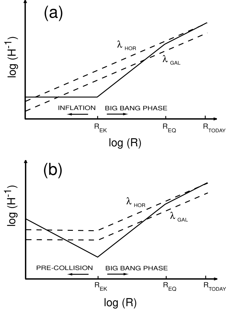
Figure 4: Sketch comparing the generation of a super-horizon spectrum of perturbations in (a) inflationary cosmology versus (b) the ekpyrotic universe. During inflation, the Hubble radius is nearly fixed and the fluctuation wavelength grows exponentially fast, causing modes to be stretched outside the horizon. In the ekpyrotic scenario, modes correspond to ripples on the moving bulk brane. The perturbations have nearly constant wavelength but the effective Hubble radius shrinks, once again causing modes to cross outside the horizon.

The comparison to inflationary cosmology is made in Figure 4. The salient feature of both models is that perturbation modes inside the Hubble horizon escape outside in the early universe and re-enter much later. However, the behavior of the scale factor and the Hubble horizon are quite different. In inflation, the wavelengths are stretched superluminally while the horizon is nearly constant. In the ekpyrotic scenario, the wavelengths are nearly constant while the horizon shrinks.

It remains to show that we can obtain a spectrum which is scale-invariant. Writing the equation for the perturbations in the form of Eq. (56) is useful since one can read off from it the spectral slope of the power spectrum. It is determined by the value of $(\ddot{a}_{pert}/a_{pert})\tau^{2}$. In particular, one obtains a scale-invariant spectrum if $(\ddot{a}_{pert}/a_{pert})\tau^{2}=2$ when the modes observed on the CMB cross outside the horizon. (Note that in usual 4d cosmology, this is achieved for an expanding de Sitter universe with $a\propto-\tau^{-1}$ or a contracting matter-dominated universe with $a\propto\tau^{2}$.) Combining Eqs. (54) and (57), we find

$$\frac{\ddot{a}_{pert}}{a_{pert}}\tau^{2}=D_{0}^{-3}\left(\alpha\frac{dV_{0}}{dY_{0}}-D_{0}\frac{d^{2}V_{0}}{dY_{0}^{2}}\right)\left[\int_{0}^{Y}\frac{D(Y^{\prime})dY^{\prime}}{\sqrt{2(E-V(Y^{\prime}))}}\right]^{2}.$$ (63)

The spectrum will be scale-invariant if the right hand side of Eq. (63) equals 2 when the modes of interest cross outside the horizon.

As a simple example, consider the case where $|V(Y)|\ll|E|$. Eq. (63) then generically gives $(\ddot{a}_{pert}/a_{pert})\tau^{2}\ll 1$. This leads to a density spectrum of the form $|\delta_{k}|\sim k$, which is thus unacceptably blue. (A similar calculation was repeated for other set-ups such as Randall-Sundrum and the solutions presented in Ref. References. It was found that none of these solutions predict a scale-invariant spectrum of fluctuations when $V$ is turned off.) It is therefore crucial to add a potential in order to obtain a scale-invariant spectrum of density fluctuations.

V.2.2 A successful example: The exponential potential

We can add a potential $V(Y)$ of the form that might result from the exchange of wrapped M2-branes. We would like to think of $V$ as the potential derived from the superpotential $W$ for the modulus $Y$ in the 4d low energy theory. Typically, superpotentials for such moduli are of exponential form, for example,

$$W\sim e^{-cY},$$ (64)

where $c$ is a positive parameter with dimension of mass. The corresponding potential is constructed from $W$ and the Kähler potential $K$ according to the usual prescription

$$V=e^{K/M_{pl}^{2}}\left[K^{ij}D_{i}W\,\bar{D_{j}W}-\frac{3}{M_{pl}^{2}}W\bar{W}\right].$$ (65)

where $D_{i}=\partial/\partial\phi^{i}+K_{i}/M_{pl}^{2}$ is the Kähler covariant derivative, $K_{i}=\partial K/\partial\phi^{i}$, $K_{ij}=\partial^{2}K/\partial\phi^{i}\partial\phi^{j}$ and a sum over each superfield $\phi_{i}$ is implicit. Eqs. (64) and (65) imply that $V$ decays exponentially with $Y$. For the purpose of this paper, we shall not worry about the exact form of the superpotential in heterotic M-theory. Rather, it will suffice to perform the calculation using a simple exponential potential, namely

$$V(Y)=-ve^{-m\alpha Y},$$ (66)

where $v$ and $m$ are positive, dimensionless constants. In this paper, it is convenient to parameterize the exponent in terms of $\alpha$. Note that, in the case where the potential is generated by the exchange of wrapped M2-branes, the parameter $m$ is of the form $m=cT_{3}\nu/\alpha$, where $c$ is a constant, $T_{3}$ is the tension of the M2-brane, and $\nu$ is the volume of the curve on which it is wrapped. The potential defined in Eq. (66) is shown in Figure 2. The perturbation modes of interest are those which are within the current Hubble horizon. As the wavelengths corresponding to those modes passed outside the effective Hubble horizon on the moving bulk-brane, the amplitudes became fixed. Scale invariance will require $mD\gg 1$ during this period. (In section V.2.3, we shall generalize this condition for an arbitrary potential $V$.)

We have already seen at the end of Section V.2.1 that, if the potential $V$ is negligible compared to $E$, the spectrum of fluctuations is not scale-invariant. Hence, we consider the limit where $|E|\ll|V_{0}|$. This condition, as seen from the equation of motion for $Y_{0}$, Eq. (53), is satisfied if $\dot{Y}_{0}=0$ initially, or, equivalently, if the bulk brane begins nearly at rest. For the brane to be nearly at rest, one must have $|E|\approx|V_{0}|$ initially. As the brane traverses the fifth dimension, $|V|$ increases exponentially, whereas $E$ is constant. Hence, the condition $|E|\ll|V_{0}|$ is automatically satisfied. The bulk brane beginning nearly at rest is precisely what we expect for a nearly BPS initial state.

Applying the condition $|E|\ll|V_{0}|$, Eq. (54) reduces to

$$\tau^{2}\approx\frac{1}{2v}\left[\int_{0}^{Y_{0}}D(Y^{\prime})e^{m\alpha Y^{\prime}/2}dY^{\prime}\right]^{2}\approx\frac{2D_{0}^{2}}{m^{2}\alpha^{2}ve^{-m\alpha Y_{0}}}\left(1-\frac{2}{mD_{0}}\right),$$ (67)

where we have neglected the endpoint contribution at $Y=0$. On the other hand, Eq. (57) gives

$$\frac{\ddot{a}_{pert}}{a_{pert}}=\frac{m^{2}\alpha^{2}ve^{-m\alpha Y_{0}}}{D_{0}^{2}}\left(1+\frac{1}{mD_{0}}\right).$$ (68)

Combining the above two expressions yields

$$\frac{\ddot{a}_{pert}}{a_{pert}}\tau^{2}=2\left(1+\frac{1}{mD_{0}}\right)\left(1-\frac{2}{mD_{0}}\right).$$ (69)

The right hand side of Eq. (69) is approximately equal to 2 in the limit of large $mD_{0}$. Hence, the exponential potential of Eq. (66) results in a nearly scale-invariant spectrum of perturbations provided that $|E|\ll|V_{0}|$ and $mD_{0}\gg 1$ are satisfied when modes pass outside the effective Hubble horizon. Note that it would be exceedingly difficult to maintain $(\ddot{a}_{pert}/a_{pert})\tau^{2}$ close to almost any other value than 2. It is indeed fortunate that scale-invariance is the desired result because obtaining a different spectral index from the ekpyrotic scenario would be highly problematic.

We next compute the perturbation amplitude, by using Eq. (56) to calculate $|\Delta Y_{k}|$. As shown above, in order for the spectrum to be scale-invariant, the conditions $|E|\ll|V_{0}|$ and $mD_{0}\gg 1$ must be satisfied when wavelengths pass outside the horizon. These conditions can be relaxed once the mode is well outside the horizon. For example, we will assume no restrictions on $mC$, the value of $mD_{0}$ at $y=0$.

In the limit that $mD_{0}\gg 1$ when the relevant modes cross outside the horizon, Eq. (56) reduces to

$$x^{2}\frac{d^{2}f_{\vec{k}}}{dx^{2}}-\left[2-x^{2}\right]f_{\vec{k}}=0,$$ (70)

with solution

$$f_{k}=x^{1/2}\left(C_{1}(k)J_{3/2}(x)+C_{2}(k)J_{-3/2}(x)\right),$$ (71)

where $J_{\pm 3/2}$ are Bessel functions. The coefficients $C_{1}(k)$ and $C_{2}(k)$ are fixed by requiring that modes well-within the horizon (i.e., $x\gg 1$) be Minkowskian vacuum fluctuations, that is

$$f_{\vec{k}}=\frac{1}{\sqrt{6k\beta M_{5}^{3}B}}e^{-ik\tau}\;\;\;{\rm for}\;\;x\gg 1.$$ (72)

(Note that the factor of $\sqrt{6\beta M_{5}^{3}B}$ in Eq. (72) arises when we change variables from $Y$ to a canonically-normalized scalar field.) Using this initial condition, we find the following rms amplitude for modes outside the horizon (with $x\ll 1$)

$$\Delta f_{k}\equiv\frac{k^{3/2}f_{k}}{(2\pi)^{3/2}}=\frac{-i}{(-\tau)(2\pi)^{3/2}\sqrt{6\beta M_{5}^{3}B}}.$$ (73)

Substituting Eq. (67) and using $f_{k}=D_{0}\delta Y_{k}$, we find

$$\Delta Y_{k}=\frac{m\alpha}{2(2\pi)^{3/2}\sqrt{3\beta M_{5}^{3}B}}\frac{\sqrt{ve^{-m\alpha Y_{0}}}}{D_{0}^{2}}.$$ (74)

Finally, we define the time-delay $\Delta\tau(k)$ by

$$|\Delta\tau(k)|=\left|\frac{\Delta Y_{k}}{\dot{Y_{0}}}\right|=\frac{m^{2}\alpha}{16\pi^{3/2}\sqrt{3\beta M_{5}^{3}B}}\left(\frac{2}{mD_{0}}\right),$$ (75)

where we have used the equation of motion for $Y_{0}$, Eq. (53). Note that the time-dependence of $\Delta\tau(k)$ is mild, a necessary condition for the validity of the time-delay formalism. The factor of $mD_{0}\equiv mD(Y_{0}(\tau))$ is to be evaluated at time $\tau$ when a given mode crosses outside the horizon during the motion of the bulk brane. Let $D_{k}$ denote the value of $D_{0}$ at horizon crossing for mode $k$. Since horizon crossing occurs when $x=1$, or, equivalently, when $(-\tau)=k^{-1}$, Eq. (67) gives

$$D_{k}\approx\frac{2}{m}\log\left(\frac{m^{2}\alpha}{2k}\sqrt{\frac{ve^{mC}}{2}}\right).$$ (76)

Substituting Eqs. (75) and (76) into Eq. (51), we find

$$|\delta_{k}|=\frac{\alpha^{2}m^{4}\sqrt{2v}}{4\pi^{3/2}\sqrt{3\beta M_{5}^{3}B}(mC+2)}\left(\frac{2}{mD_{k}}\right).$$ (77)

This expression for $|\delta_{k}|$ increases gradually with increasing $k$, corresponding to a spectrum tilted slightly towards the blue. The blue tilt is due to the fact that, in this example, $D$ is decreasing as the brane moves. That is, the spectral index,

$$n_{s}\equiv 1+\frac{d\log|\delta_{k}|^{2}}{d\log k}\approx 1+\frac{4}{mD_{k}},$$ (78)

exceeds unity. The current CMB data constrains the spectral index to lie in the range about $0.8<n_{s}<1.2$. Therefore, for our results to be consistent with experiments, we must have

$$mD_{k}>20,$$ (79)

a constraint that is easily satisfied.

V.2.3 General potential

As a second example, consider the power-law potential

$$V(Y)=-vD(Y)^{q}=-v(\alpha Y+C)^{q},$$ (80)

where $v>0$ and $q<0$ are constants. In this case, Eq. (63) gives

$$\frac{\ddot{a}_{pert}}{a_{pert}}\tau^{2}\approx 2\frac{\left(1-\frac{2}{q}\right)}{\left(1-\frac{4}{q}\right)^{2}}\approx 2$$ (81)

for $|q|\gg 1$. Hence, a power-law potential can also lead to a nearly scale-invariant spectrum provided that its exponent is sufficiently large. (The smaller is the value of $|q|$, the bluer is the spectrum.)

We can straightforwardly extend our analysis to an arbitrary potential $V(Y)$. Let us suppose that $V(Y)$ satisfies

$$\left|D(Y)\frac{dV}{dY}\right|\gg\alpha|V(Y)|$$

$$\left|D(Y)\frac{d^{2}V}{dY^{2}}\right|\gg\alpha\left|\frac{dV}{dY}\right|,$$ (82)

(For the exponential potential, $V(Y)=-ve^{-m\alpha Y}$, these two conditions amount to $mD\gg 1$.) Then, Eq. (63) reduces to

$$\frac{\ddot{a}_{pert}}{a_{pert}}\tau^{2}\approx 2\left(\frac{VV^{\prime\prime}}{V^{\prime 2}}\right).$$ (83)

Hence, the conditions for scale invariance are Eqs. (82) as well as

$$\frac{VV^{\prime\prime}}{V^{\prime 2}}\approx 1.$$ (84)

V.3 Gravitational waves from colliding branes

In inflationary cosmology, the analysis of tensor (gravitational wave) perturbations follows closely the analysis of scalar (energy density) perturbations [47]. Metric fluctuations can be divided into two polarizations, each of which acts like a massless scalar field evolving in the same cosmic background as the inflaton. Hence, it is not surprising that the spectrum of tensor fluctuations has nearly the same scale-invariant spectral shape as the scalar spectrum.

In the ekpyrotic scenario, the relationship between scalar and tensor perturbations is less direct. The excitations that produce scalar perturbations are ripples on the moving brane, which are directly dependent on the rate at which the brane traverses the fifth dimension and the potential that drives it. The tensor fluctuations, on the other hand, are excitations of the gravitational field, which lives in the bulk. (The moving brane itself does not support tensor fluctuations.) The net result is a different effective scale factor in the fluctuation equation of motion for the tensor modes than for the scalar modes.

We shall briefly outline the derivation here, with more details to follow in our more formal paper on perturbations [48]. If $\bar{g}_{\mu\nu}$ is the unperturbed, homogeneous metric (see Eq. (13) with $A$ and $N$ functions of time), the perturbed 5d metric can be written as

$$g_{\mu\nu}=\bar{g}_{\mu\nu}+A^{2}(t)D(y,t)h_{\mu\nu}(\vec{x},t),$$ (85)

where $\mu,\nu=0,\dots 3$. Note that since we shall work at the level of the 4d effective theory, we can treat the tensor perturbations $h_{\mu\nu}$ as functions of $\vec{x}$ and $t$ only. We are interested in the tensor perturbations which satisfy the conditions: $h_{0\mu}=0$, $h^{i}_{j}=0$, and $\partial^{i}h_{ij}=0$. The perturbed 5d Einstein action to quadratic order is

$$S_{fluct}^{T}\equiv\frac{M_{5}^{3}}{2}\int d^{5}x\sqrt{-g}R=\frac{M_{5}^{2}}{8}\int d^{4}xa^{2}(\dot{h}^{\mu}_{\;\nu}\dot{h}^{\;\nu}_{\mu}-\partial_{i}h^{\mu}_{\;\nu}\partial^{i}h^{\;\nu}_{\mu})$$ (86)

where the second expression is obtained by integrating over $y$. The tensor action is analogous to the scalar action given in Eq. (55). From the action, we can derive the tensor analogue of the scalar fluctuation equation of motion, Eq. (56)

$$x^{2}\frac{d^{2}f_{\vec{k}}^{T}}{dx^{2}}-\left[\frac{\ddot{a}}{a}\tau^{2}-x^{2}\right]f_{\vec{k}}^{T}=0,$$ (87)

where

$$h^{\mu}_{\;\nu}\equiv\int\frac{d^{3}k}{(2\pi)^{3}}\epsilon^{\mu}_{\;\nu}h_{k}(\tau)$$ (88)

and

$$f_{\vec{k}}^{T}\equiv a\,h_{\vec{k}}.$$ (89)

The critical difference between this tensor equation and the scalar fluctuation equation, Eq. (56), is that the effective scale factor $a_{pert}$ in Eq. (56) has been replaced by $a$. We introduced a potential to insure that $a_{pert}$ led to a nearly scale-invariant spectrum, $(\ddot{a}_{pert}/a_{pert})\tau^{2}\approx 2$. However, $a(\tau)$ in the tensor equation is approximately constant (recall that $a=(BI_{3}^{(0)}M_{5})^{1/2}+{\cal O}(\beta/\alpha)$). Consequently, the root mean square tensor fluctuation amplitude,

$$|\Delta h_{\vec{k}}|\equiv\frac{k^{3/2}h_{\vec{k}}}{(2\pi)^{3/2}}\sim\frac{k}{(2\pi)^{3/2}}.$$ (90)

is not scale-invariant. Rather, the tensor spectrum is tilted strongly to the blue. Fitting the mean square amplitude to a scale-free form, $\sim k^{n_{T}}$, where $n_{T}$ is the conventional tensor spectral index, the spectrum above corresponds to $n_{T}=2$, compared to the inflationary prediction, $n_{T}\leq 0$.

The tensor spectrum is a prediction that clearly distinguishes the ekpyrotic scenario from inflationary cosmology. In both cases, for the same Hubble parameter at reheating (for inflation) or collision, $H_{c}$, the mode with wavelength of order $H_{c}^{-1}$ has similar amplitude, $H_{c}/M_{pl}$, where $M_{pl}$ is the 4d Planck mass. The wavelength of this mode today is roughly 60 e-folds smaller than the current Hubble radius. Hence, if we extrapolate from this wavelength to one comparable to the present Hubble radius, $H_{0}^{-1}$, the inflationary prediction is that the amplitude is nearly the same (since the spectrum is nearly scale-invariant), whereas the blue spectrum computed above predicts that the amplitude is exponentially small. Hence, the search for a gravitational wave signal using the CMB polarization on horizon scales becomes a key test for our proposal. Future gravitational wave detectors, beyond the presently planned LISA and LIGO projects, may also someday detect the stochastic background of gravitational waves as well. Observing a nearly scale invariant primordial gravitational wave background falsifies the ekpyrotic scenario and is consistent with inflation.

VI Conclusions

VI.1 Recapitulation

Conceptually, the ekpyrotic scenario appears to be simple: a bulk brane strikes our visible brane and a hot big bang universe is born. In actuality, to accomplish the transformation from a cold, nearly BPS state into an expanding, hot universe with nearly scale-invariant density perturbations without invoking inflation requires a series of seemingly incongruous conditions. Remarkably, these conditions can be satisfied simultaneously in heterotic M-theory.

First, the gravitational backreaction due to the kinetic energy of the bulk brane must trigger cosmic expansion. In 4d gravity, kinetic energy usually causes cosmic deceleration and, if the initial state is static, it triggers contraction. Second, the total energy of the brane has to grow by drawing energy from the gravitational field since, otherwise, the total bulk brane energy before and after collision is zero and there is no radiation. In 4d gravity, this blue shift effect occurs if the universe is contracting, but here it occurs even though the scale factor on the visible brane is expanding. Third, the scalar (energy density) fluctuations must be nearly scale-invariant. Although scale-invariance is ordinarily associated with inflation, here we have shown that a scale-invariant spectrum results even though the universe is quasi-static. The only requirement is a bulk brane potential whose magnitude increases by an exponential factor as the brane traverses the bulk. Potentials of this type occur in string theory. (Our analysis suggests that scale-invariance is especially favored in the 5d theory. It occurs for rather simple, physically-motivated potentials, whereas more general spectral shapes are difficult to obtain.) Fourth, the tensor fluctuation spectrum is not scale-invariant but, rather, strongly tilted towards the blue, providing an observational signature that distinguishes the ekpyrotic scenario from inflationary cosmology.

In the context of 4d gravity, some of these features suggest slow expansion, others superluminal expansion, yet others contraction. How do we obtain all of these features simultaneously? All of this is possible in our 5d theory because the role of gravity in the equations of motion for the expansion, the brane motion, and the scalar and tensor fluctuations is played by different combinations of moduli fields for each equation. That is, each equation is similar to the corresponding equation for a scalar field in a 4d FRW background except that the scale factor $a(t)$ is replaced by some function of the moduli fields that differs for each physical quantity. Some combinations increase with time, mimicking an expanding universe, and others decrease, mimicking a contracting universe. The remarkable result is that just the right combinations of moduli occur in heterotic M-theory to produce the behavior required for a viable cosmological scenario.

An observer at any surface of fixed $y$ has a scale factor equal to $AD^{1/2}(y,\tau)$ (see Eq. (13)), which is expanding as the bulk brane collides with the visible brane. In Eq. (25), which describes the time variation of the total energy of the bulk brane, the role of the scale factor is played by $a$, which is contracting. The contraction produces the blue shift or increase in the total energy so that, upon collision, there is excess kinetic energy that can be converted to radiation. The scalar fluctuations are ripples in the bulk brane surface that evolve as if the scale factor were $a_{pert}$ in Eq. (56), corresponding to a contracting effective Hubble radius. We have identified simple criteria for the potential which result in a scale-invariant spectrum. The tensor fluctuation spectrum naturally differs from the scalar spectrum because tensor fluctuations occur in the bulk volume rather than on the brane surface. The effective scale factor for the tensor fluctuations is $a$, rather than $a_{pert}$. The differences account for the fact that the scalar spectrum is scale-invariant, whereas the tensor spectrum is tilted strongly to the blue.

A useful mnemonic for recalling the difference between the scalar and tensor fluctuation spectra in our scenario is to consider the equivalent relations for inflationary cosmology, but with the inflaton scalar field replaced by $Y$. For the scalar fluctuations, the amplitude is

$$\delta_{S}\sim H\left(\frac{\Delta Y}{\dot{Y}}\right)_{k=H}$$ (91)

and the tensor fluctuation amplitude is

$$\delta_{T}\sim\left(\frac{H}{M_{pl}}\right)_{k=H},$$ (92)

where $M_{pl}$ is the 4d Planck mass, $\Delta Y$ is the fluctuation amplitude for $Y$, and the subscript means that the expressions are to be evaluated when the wavenumber of a given mode is equal to the inverse Hubble radius $H$ as it passes beyond the horizon. For inflation, $H$, $\Delta Y$ and $\dot{Y}$ are nearly constant, so $\delta_{S}$ and $\delta_{T}$ are both nearly scale-invariant. For the ekpyrotic scenario, $\Delta Y$ and $\dot{Y}$ are both strongly time-varying. However, for an exponential potential $V(Y)$ as is naturally generated by non-perturbative exchange of M2-branes, the time-variation in the ratio $\Delta Y/\dot{Y}$ in the expression for $\delta_{S}$ nearly cancels. Consequently, the ratio is nearly constant and the resulting spectrum is nearly scale-invariant. However, $\delta_{T}$ involves only $H$, which is increasing with time as smaller and smaller wavelength modes pass beyond the horizon. This accounts for the fact that the spectrum is blue.

As a specific fully-worked example, consider the case of an exponential bulk brane potential, $V(Y)=-v\,{\rm exp}(-m\alpha Y)$, as discussed in Section V.2.2. We have computed the ekpyrotic temperature at the beginning of the hot big bang phase (Eq. (32)),

$$\frac{T}{M_{pl}}\approx\frac{3^{3/4}(2v)^{1/4}}{(I_{3}M_{5})^{1/2}(\alpha R+C)^{1/4}}\left(\frac{M_{5}}{M_{pl}}\right)^{1/2}\left(\frac{\beta}{\alpha}\right)^{1/2}\frac{(mC+2)^{1/2}}{m}.$$ (93)

In terms of this temperature, the scalar (energy density) fluctuation amplitude in Eq. (77) can be rewritten as

$$|\delta_{k}|=\frac{m^{6}(I_{3}\alpha)^{3/2}}{36\pi^{3/2}(mC+2)^{2}}\left(\frac{\alpha}{\beta}\right)^{3/2}\frac{2}{mD_{k}}\left(\frac{T}{M_{pl}}\right)^{2}.$$ (94)

A simple example which satisfies all constraints is $\alpha=2000M_{5}$, $\beta=M_{5}$, $B=10^{-4}$, $C=1000$, $R=M_{5}^{-1}$, $m=0.1$, and $v=10^{-8}$, all of which are plausible values. In this example, $D_{k}$ (the value of $D$ at horizon crossing) is of order $10^{3}$. Then, we find that $M_{5}\sim 10^{-2}\,M_{pl}$; the ekpyrotic temperature is $T\sim 10^{-8}\,M_{pl}$; and the scalar perturbation amplitude is $|\delta_{k}|\sim 10^{-5}$. Note that the ekpyrotic temperature, the maximal temperature of the hot big bang phase, tends to be small compared to the Planck or unification scale. This is a characteristic feature of the model. With these parameters, the magnitude of the potential energy density at collision is $(10^{-6}M_{pl})^{4}$. This corresponds to a characteristic energy scale for the potential of $10^{13}$ GeV. Finally, note that these values are consistent with Hořava-Witten phenomenology. For instance, the proper distance between the branes is $R_{proper}^{-1}\sim 10^{-5}M_{pl}$. If we further assume that the characteristic length scale $L_{CY}$ of the Calabi-Yau three-fold is approximately 10 times smaller than $R_{proper}$ (in order for the five-dimensional effective theory to be valid), then we get agreement with the values of $R_{proper}$, $L_{CY}$, and the 11d Planck mass $M_{11}$ inferred by Witten in Ref. References in matching the gauge and gravitational coupling constants.

While we are pleased that the numerical constraints from cosmology and those from Hořava-Witten phenomenology can be simultaneously satisfied, we should emphasize that there is a lot of flexibility in terms of parameters. For instance, in the above example the ratio $\beta/\alpha$ was chosen to be of order $10^{-3}$. However, one can easily make this ratio as large as $1/10$ if one wishes. For example, choosing $\alpha=200M_{5}$, $\beta=20M_{5}$, $B=10^{-2}$, $C=100$, $R=M_{5}^{-1}$, $m=1$, and $v=10^{-10}$ results in $T\sim 10^{-7}\,M_{pl}$, $|\delta_{k}|\sim 10^{-5}$, $M_{5}\sim 10^{-2}\,M_{pl}$, $R_{proper}^{-1}\sim 10^{-5}M_{pl}$, and characteristic energy scale for the potential of $10^{14}$ GeV. The value of $R_{proper}$ could also take a significantly different value, if one wishes, and there would still be enough freedom to obtain reasonable ekpyrotic temperature and fluctuations. We can also imagine applying the same ideas in a different brane world context, such as AdS, and still obtaining a successful scenario from a cosmological point-of-view. The challenge, of course, is to figure out how to break supersymmetry, obtain a correct phenomenology and stabilize moduli. Here we have presumed that this challenge can be met, and have shown through examples how the brane world approach to particle phenomenology might be combined with new ideas in cosmology to obtain a successful picture of the early Universe.

VI.2 Colliding Branes and Inflationary Cosmology

We have laid out a detailed cosmological scenario that offers a resolution of the flatness, horizon, and monopole problems and generates a nearly scale-invariant spectrum of energy density perturbations based on concepts that derive naturally from extra dimensions, branes, and heterotic M-theory. The key conceptual difference from inflation is how the universe begins. In the usual approaches to inflationary cosmology, as in standard big bang cosmology, the universe begins with a cosmological singularity. The universe emerges in a high energy state with no particular symmetry and rapidly expanding. Superluminal expansion is invoked to smooth out and flatten the emerging state. The ekpyrotic scenario introduces a different philosophy in which the universe begins in a non-singular, infinite, empty, quasi-static state of high symmetry. Superluminal expansion is not needed because the BPS vacuum state is flat and smooth. Brane collision can account for the matter-radiation energy and primordial density perturbations.

Let us briefly summarize how the ekpyrotic scenario addresses the various cosmological problems:

• Causal Horizon Problem: In the ekpyrotic scenario, the local temperature and density are set by the collision of the visible brane and bulk brane, which acts as a non-local event that occurs nearly simultaneously over a region much larger than the Hubble horizon.

• Flatness Problem: The universe is assumed to begin in a nearly BPS ground state. The BPS state corresponds to a spatially-flat geometry. The process of bulk brane formation/nucleation and propagation maintains flatness. (We do not demand that the initial state be globally BPS to resolve the horizon and flatness problems. It suffices that the universe be flat and homogeneous on scales up to the (causal) particle horizon, as should occur naturally beginning from more general initial conditions. In the ekpyrotic scenario, because the bulk brane motion is extremely slow, the particle horizon at collision is exponentially large compared to the Hubble horizon, where the latter is set by the radiation temperature after collision.)

• Monopole Problem: The hot big bang epoch commences when the bulk brane collides with the visible brane and heats the universe to a finite temperature. Provided the temperature is less than the monopole mass, the monopole abundance will be negligible.

• Inhomogeneity Problem: Quantum fluctuations generate ripples in the bulk brane as it traverses the bulk. Due to the ripples, collision and thermalization occur at varying times across the visible brane, resulting in fluctuations in energy density and gravitational waves.

Both the ekpyrotic scenario and inflationary cosmology have the feature that the causal horizon is exponentially greater than the Hubble horizon. In inflation, superluminal expansion rapidly stretches the causal horizon while the Hubble horizon is nearly fixed. In the colliding brane picture, the collision of the bulk brane acts as a non-local interaction that causally links regions separated by much more than a Hubble distance.

Both the inflationary and ekpyrotic scenarios produce a nearly scale-invariant spectrum of energy density perturbations from quantum fluctuations. For inflation, quantum fluctuations are stretched beyond the Hubble horizon as the universe expands superluminally. For the ekpyrotic universe, the Hubble horizon is shrinking compared to the quantum fluctuations as the universe contracts very slowly. The equations describing the evolution of perturbations are (nearly) equivalent in the two cases (see discussion of Eq. (56)), even though, one describes an expanding de Sitter phase and the other a contracting pressureless phase. The similar equations account for why both lead to scale-invariant spectra for density perturbations even though the mechanisms are different.

From the point-of-view of an observer on the stationary orbifold planes, the universe is expanding as the branes collide. The bulk brane is what causes their expansion, a gravitational backreaction effect due to its motion. The expansion is very slow as the brane moves across the fifth dimension, but assumes the usual big bang rate after collision and thermalization.

One might hope that the ekpyrotic scenario avoids the tuning problems required in standard inflation in order to obtain an acceptable perturbation spectrum. Thus far, the situation is unclear. We found that we had to introduce a flat potential for the bulk brane that is roughly similar to the flat inflaton potential used in standard inflation. The form is also qualitatively consistent with non-perturbative potentials that arise in M-theory. Perhaps the potential parameters needed for our scenario will be shown to arise naturally. However, it should also be noted that the reasons for introducing the potential in the ekpyrotic scenario are different from the case of inflation. In our case, the need for a flat potential is linked to the precise form of the background static BPS solution of Lukas, Ovrut and Waldram used in this paper. Perhaps there exist other initial conditions which avoid the need for flat potentials altogether.

Although inflationary cosmology and the colliding brane picture both produce a nearly scale-invariant spectrum of perturbations, the deviation from scale-invariance differs due to the fact that the background felt by the perturbations is expanding in one scenario and contracting in the other. In standard inflationary cosmology, the spectrum of scalar (density) and tensor (gravitational wave) perturbations is typically red (amplitude decreases as wavelength decreases).[51] The amplitude of a given mode is proportional to the Hubble parameter when the wavelength is stretched beyond the horizon. The Hubble parameter decreases (slowly) in an expanding, inflating universe. Since smaller wavelength modes stretch beyond the horizon at later times when the Hubble parameter is smaller, they have a smaller amplitude, resulting in a red spectrum. The degree of redness is expressed in terms of a “spectral index,’[52] $n_{S,T}$ for scalar and tensor perturbations respectively, where $n_{S}-1=n_{T}=0$ is defined as precise scale-invariance, and $n_{S}-1<0$ and $n_{T}<0$ correspond to red spectra. In the examples of the ekpyrotic scenario discussed here, the apparent Hubble radius for an observer on the bulk brane is shrinking. Consequently, the corresponding spectra are blue. By introducing a potential for the bulk brane (dependent, say, on its position $Y$), the density perturbation spectrum can be made nearly scale-invariant, slightly blue ($n_{S}-1>0$) in our examples. On the other hand, the gravitational wave spectrum is unaffected by the potential and is strongly blue $n_{T}\approx 2$.

For energy density perturbations, there are exceptional cases where inflation can give a blue spectrum [53]. The blue spectrum arises because the density perturbation amplitude is not only proportional to the Hubble parameter, but also inversely proportional to the kinetic energy of the inflaton. As inflation proceeds, the Hubble parameter decreases and, in most models, the inflaton kinetic energy increases; so both effects tend to make the spectrum red. But models can be rigged where the Hubble parameter decreases, as usual, but the inflaton kinetic energy decreases more rapidly. In that case, the spectrum is blue. Similarly, it is possible to get a red spectrum in the ekpyrotic model, for example, if the bulk brane moves in the direction of increasing warp factor.[54] Hence, observing a red or blue density spectrum is not a decisive test for distinguishing the two scenarios.

However, the gravitational wave spectrum for inflation is always red — the amplitude depends only on the Hubble parameter — and so observing a strongly blue gravitational wave spectrum, as predicted by the ekpyrotic scenario, is a key test. The cosmic microwave background polarization is one method of detecting the presence of primordial gravitational waves with wavelengths comparable to the Hubble horizon today. For the slightly red spectrum of inflationary cosmology, the gravitational wave amplitude may be large enough to be detected. However, for a strongly blue spectrum, the signal at large length scales is exponentially small and undetectable. Hence, the detection of gravitational waves in the microwave background polarization would falsify our scenario. Currently planned gravitational wave detectors, such as LIGO and LISA, are not sensitive enough to detect the gravitational waves from inflation or from our scenario. However, future detectors may discover the stochastic background and determine the spectral slope.

Certain aspects of our scenario are reminiscent of the novel, string-inspired, pre-big bang models introduced by Veneziano and Gasperini [18, 19]. Both assume the universe begins in a flat, empty state [20]. In both models, the gravitational wave perturbation spectrum is blue [55]. However, the structure, ingredients, dynamics and predictions of the two models are very different. The pre-big bang scenario does not entail extra dimensions or branes in a direct way. The pre-big bang begins with a semi-infinite period of contraction which is superluminal (deflation). This period ends in a global singularity in which the Hubble constant becomes infinite. Matching across this singularity is the biggest challenge facing the pre-big bang model. If it is possible at all, it can only be at the string scale where non-perturbative stringy effects are large and difficult to compute. In our model, matching to the universe after the bulk-boundary collision is complex, and will require calculations in the five dimensional theory which we have not studied here. But the collision event itself is nonsingular and it is an important advantage of our scenario that it only involves physics taking place at low energies, which is in principle describable using the effective low energy Lagrangian. A second difference is that all expansion and contraction are subluminal in our model. Finally, in the simplest renditions of pre-big bang, the fluctuation spectrum is so strongly tilted to the blue relative to a scale invariant spectrum that current observational bounds on the microwave background anisotropy are violated. The ekpyrotic scenario obtains a spectrum that is consistent with current observations.

To summarize, we have presented a novel scenario for the beginning of the hot big bang universe, within a framework consistent with string theory and supergravity. The universe begins in the simplest state possible, one which is cold, nearly BPS, and nearly vacuous. At some time, a bulk brane exists or is nucleated in the vicinity of the hidden brane (through a small instanton phase transition), and begins to move towards the visible brane. The bulk brane eventually collides with the visible brane and is absorbed in a small instanton phase transition. This transition may change the gauge group on the visible brane to the standard model gauge group, as well as create three families of light quarks and leptons. At the moment of collision, a fraction of the kinetic energy of the brane is converted to thermal excitations of the light degrees of freedom on the visible brane, causing the universe to enter an FRW radiation-dominated phase. Furthermore, ripples on the bulk brane imprint a spectrum of energy density fluctuations consistent with current observations and which provides the seeds for structure formation. While parts of our scenario remain speculative at present (such as the dynamics of the small instanton phase transition), it is our hope that advances in heterotic M-theory will eventually allow us to solidify the components of our cosmological model. For the moment, we consider our scenario as a first step towards a new, testable model for the early universe consistent with current cosmological observations and fully-motivated by string theory.

Acknowledgments
We would like to thank C.P. Burgess, S. Gubser, J. Maldacena, M. Bucher, N. Seiberg, D. Spergel, D. Waldram and T. Wiseman for helpful discussions, and Katharina Volk and J. Katz for introducing us to ancient cosmology and ekpyrosis. We thank R. Kallosh et al. [54, 56] for pointing out minor typographical errors in the manuscript. We would also like to thank the Director and staff of the Newton Institute for Mathematical Sciences, where this work was initiated, and the organizers of the String Cosmology Workshop at the the Pacific Institute for Mathematical Sciences (Vancouver) where some of this work was carried forth. This work was supported in part by the Natural Sciences and Engineering Research Council of Canada (JK), the US Department of Energy grants DE-FG02-91ER40671 (JK and PJS) and DE-AC02-76-03071 (BAO), and by PPARC-UK (NT).

References

- [1] A. H. Guth, Phys. Rev. D 23 (1981) 347.
- [2] A. D. Linde, Phys. Lett. B 108 (1982) 389; A. Albrecht and P. J. Steinhardt, Phys. Rev. Lett. 48 (1982) 1220.
- [3] V.A. Ruybakov and M.R. Shaposhnikov, Phys. Lett. B 125 (1983) 136.
- [4] K. Akama, Lect. Notes Phys. 176 (1982) 267.
- [5] P. Hořava and E. Witten, Nucl. Phys. B460 (1996) 506; B475 (1996) 94.
- [6] A. Lukas, B.A. Ovrut and D. Waldram, Nucl. Phys. B532 (1998) 43; Phys. Rev. D 57 (1998) 7529; A. Lukas, B.A. Ovrut, K.S. Stelle and D. Waldram, Phys. Rev. D 59 086001 (1999).
- [7] J. Lykken, E. Poppitz and S.P. Trivedi, Phys. Lett. B 416 (1998) 286; Nucl. Phys. B543 (1999) 105; Nucl. Phys. B520 (1998) 51.
- [8] L.E. Ibanez, C. Mu oz and S. Rigolin, Nucl. Phys. B553 (1999) 43; G. Aldazabal, L.E. Ibanez and F. Quevedo, JHEP 0001 (2000) 031; JHEP 0002 (2000) 015.
- [9] G. Shiu and S.-H. Henry Tye, Phys. Rev. D 58 (1998) 106007; Z. Kakushadze and S.-H. Henry Tye, Nucl. Phys. B548 (1999) 180.
- [10] L. Randall and R. Sundrum, Nucl. Phys. B557 (1999) 79; Phys. Rev. Lett. 83 (1999) 3370; Phys. Rev. Lett. 83 (1999) 4690.
- [11] N. Arkani-Hamed, S. Dimopoulos and G. Dvali, Phys. Lett. B 429 (1998) 263; Phys. Rev. D 59 (1999) 086004; I. Antoniadis, N. Arkani-Hamed, S. Dimopoulos and G. Dvali, Phys. Lett. B 436 (1998) 257; N. Arkani-Hamed, S. Dimopoulos and J. March-Russell, Phys.Rev. D 63 (2001) 064020; N. Arkani-Hamed, S. Dimopoulos, G. Dvali and N. Kaloper, Phys. Rev. Lett. 84 (2000) 586-589; JHEP 0012 (2000) 010.
- [12] E.B. Bogomol’nyi, Sov. J. Nucl. Phys. 24 (1976) 449; M.K. Prasad and C.M. Sommerfield, Phys. Rev. Lett. 35 (1975) 760.
- [13] K. Volk and J. Katz, private communication.
- [14] E.R. Harrison, Phys. Rev. D 1 (1970) 2726; Ya.B. Zel’dovich, MNRAS 160 (1972) 1p.
- [15] E. Witten, Nucl. Phys. B471 (1996) 135.
- [16] T. Banks and M. Dine, Nucl. Phys. B479 (1996) 173.
- [17] J. Khoury, B.A. Ovrut, N. Seiberg, P.J. Steinhardt and N. Turok, in preparation (2001).
- [18] G. Veneziano, Phys. Lett. B 265 (1991) 287.
- [19] M. Gasperini and G. Veneziano, Astropart. Phys. 1, (1993) 317.
- [20] A. Buonanno, T. Damour and G. Veneziano, Nucl. Phys. B 543 (1999) 275.
- [21] G. Dvali and S.-H. Henry Tye, Phys. Lett. B450 (1999) 72.
- [22] G. Dvali, Phys. Lett. B459 (1999) 489.
- [23] G. Dvali and G. Gabadadze, Phys. Lett. B460 (1999) 47.
- [24] C. Park and S.-J. Sin, Phys. Lett. B485 (2000) 239.
- [25] S.H.S. Alexander, hep-th/0105032.
- [26] T. Banks, hep-th/9911067.
- [27] A. Lukas, B.A. Ovrut and D. Waldram, Phys. Rev. D 60 (1999) 086001.
- [28] A. Lukas, B.A. Ovrut and D. Waldram, Phys. Rev. D 61 (2000) 023506.
- [29] G.D. Starkman, D. Stojkovic and M. Troden, Phys. Rev. D 63 (2001) 103511.
- [30] A. Lukas, B.A. Ovrut, K.S. Stelle and D. Waldram, Nucl. Phys. B552 (1999) 246.
- [31] A. Lukas, B.A. Ovrut and D. Waldram, Phys. Rev. D 59 (1999) 106005.
- [32] R. Donagi, A. Lukas, B.A. Ovrut and D. Waldram, JHEP 9905 (1999) 018: R. Donagi, A. Lukas, B.A. Ovrut and D. Waldram, JHEP 9906 (1999) 034: R. Donagi, B.A. Ovrut and D. Waldram, JHEP 9911 (1999) 030.
- [33] R. Donagi, B.A. Ovrut, T. Pantev and D. Waldram, hep-th/9912208; hep-th/0008008; math.AG/000801; math.AG/0008011.
- [34] See, for example: E. Caceres, V.S. Kaplunovsky and I.M. Mandelberg, Nucl. Phys. B493 (1997) 73; H.-P. Nilles and S. Steiberger, Nucl. Phys. B499 (1997) 3; I. Antoniadis and M. Quiros, Phys. Lett. B392 (1997) 61; K. Choi, Phys. Rev. D 56 (1997) 6588; Z. Lalak and S. Thomas, Nucl.Phys. B515 (1998) 55; S. Lalak, A. Lukas and B.A. Ovrut, Phys. Lett. B425 (1998) 59; A. Lukas, B.A. Ovrut and D. Waldram, Phys. Rev. D 57 (1998) 7529, Nucl. Phys. B540 (1999) 230; K. Choi, B. Kim and C. Munoz, Phys. Rev. D 57 (1998) 7521; H.-P. Nilles, M. Olechowski and M. Yamaguchi, Nucl. Phys. B530 (1998) 43; T. Li, Phys. Rev. D 57 (1998) 7539, Phys. Rev. D 59 (1999) 107902.
- [35] See, for example: J. Ellis, Z. Lalak, S. Pokorski and W. Pokorski, Nucl. Phys. B540 (1999) 149; R. Sundrum, Phys. Rev. D 59 (1999) 085009; K.R. Dienes, E. Dudas and T. Gherghetta, Nucl. Phys. B537 (1999) 47; J. Ellis, Z. Lalak and W. Pokorski, Nucl. Phys. B559 (1999) 71; K. Behrndt, Nucl. Phys. B573 (2000) 127; O. DeWolfe, D.Z. Freedman, S.S. Gubser and A. Karch, Phys. Rev. D 62 (2000) 046008; A. Lukas and K.S. Stelle, JHEP 0001 (2000) 010; K. Behrndt and S. Gukov, Nucl. Phys. B580 (2000) 225; S. Kachru, M. Schulz and E. Silverstein, Phys. Rev. D 62 (2000) 045021; M. Fabinger and P. Hořava, Nucl. Phys. B580 (2000) 243; B.R. Greene, K. Schalm and G. Shiu, Nucl. Phys. B584 (2000) 480; A. Grassi, Z. Guralnik and B.A. Ovrut, JHEP 0101 (2001) 037; P. Berglund, T. Hubsch and D. Minic, JHEP 0009 (2000) 015; P. Mayr, JHEP 0011 (2000) 013; K. Behrndt, C. Herrmann, J. Louis and S. Thomas, JHEP 0101 (2001) 011; M. Faux, D. Lust and B.A. Ovrut, Nucl. Phys. B589 (2000) 269.
- [36] G. Moore, G. Peradze and N. Saulina, hep-th/0012104.
- [37] E. Lima, B.A. Ovrut, J. Park and R. Reinbacher, hep-th/0101049; E. Lima, B.A. Ovrut and J. Park, hep-th/0102046.
- [38] J.-P. Derendinger and R. Sauser, Nucl.Phys. B598 (2001) 87.
- [39] B.A. Ovrut, T. Pantev and J. Park, JHEP 0005 (2000) 045.
- [40] N.S. Manton, Phys. Lett. B110 (1982) 54; B154 (1985) 397.
- [41] P. Binetruy, C. Deffayet and D. Langlois, hep-th/0101234.
- [42] W.D. Goldberger and M.B. Wise, Phys. Rev. Lett. 83 (1999) 4922.
- [43] A.H. Guth and S.-Y. Pi, Phys. Rev. Lett. 49 (1982) 1110.
- [44] L. Wang, V.F. Mukhanov and P.J. Steinhardt, Phys. Lett. B 414 (1997) 18.
- [45] J.M. Bardeen, P.J. Steinhardt and M.S. Turner, Phys. Rev. D 28 (1983) 679.
- [46] V.F. Mukhanov, JETP Letters 41 (1985) 493; Sov. Phys. JETP 68 (1988) 1297.
- [47] V.F. Mukhanov, H.A. Feldman and R.H. Brandenberger, Phys. Reports 215 (1992) 203.
- [48] J. Khoury, B.A. Ovrut, P.J. Steinhardt and N. Turok, in preparation (2001).
- [49] D.W. Olson, Phys. Rev. D 14 (1976) 327.
- [50] S. Kachru, M. Schulz and E. Silverstein, Phys. Rev. D 62 045021.
- [51] J.E. Lidsey et al., Rev. Mod. Phys. 69 (1997) 337.
- [52] R.L. Davis, H.M. Hodges, G.F. Smoot, P.J. Steinhardt and M.S. Turner, Phys. Rev. Lett. 69 (1992) 1856.
- [53] See, for example, A.D. Linde, Phys. Rev. D 49 (1994) 748; J. Garcia-Bellido, A.D. Linde and D. Wands, Phys. Rev. D 54 (1996) 6040.
- [54] R. Kallosh, L. Kofman and A.D. Linde, hep-th/0104073.
- [55] R. Brustein, M. Gasperini, M. Giovannini and G. Veneziano, Phys. Lett. B 361 (1995) 45.
- [56] R. Kallosh, L. Kofman, A.D. Linde and A. Tseytlin, hep-th/0106241.