CU-TP-1003

The Stability of
Noncommutative Scalar Solitons

Mark G. Jackson

Department of Physics

Columbia University

New York City, NY 10027

We determine the stability conditions for a radially symmetric noncommutative scalar soliton at finite noncommutivity parameter $\theta$. We find an intriguing relationship between the stability and existence conditions for all level-1 solutions, in that they all have nearly-vanishing stability eigenvalues at critical $\theta m^{2}$. The stability or non-stability of the system may then be determined entirely by the $\phi^{3}$ coefficient in the potential. For higher-level solutions we find an ambiguity in extrapolating solutions to finite $\theta$ which prevents us from making any general statements. For these stability may be determined by comparing the fluctuation eigenvalues to critical values which we calculate.

1 Introduction

There has recently been much interest, particularly from string theorists, in noncommutative geometry [1] [2]. Part of this interest has focused on the construction of noncommutative scalar solitons, first addressed by Gopakumar et al. [3]. Explicit constructions were carried out for $\theta=\infty$ using an isomorphism between the star product and the simple harmonic oscillator (SHO) basis. These solutions were then extrapolated to large but finite $\theta$ using the perturbed equations of motion, and some specific examples of solutions were constructed. Classical stability was addressed only as an order-of-magnitude argument: a stable solution at large $\theta$ changes mass eigenvalues by $\mathcal{O}(1/\theta)$, allowing one to conclude that angular fluctuations (in the form of $U(\infty)$ transformations) give rise to instability in some solutions while still ensuring stability against radial fluctuations. Existence of the solitons was then more thoroughly addressed in [5] and [6], where it was discovered that a potential bounded from below produces a critical $\theta$ below which there exists no solution; an unbounded potential will always yield a solution for any nonzero $\theta$. This creates a need for detailed stability analysis at finite $\theta$. In this paper we report progress in this direction.

The paper is structured as follows. In section 2 we review the construction of noncommutative solitons. In section 3 we present the tools necessary to determine radial stability of a solution. In section 4 we generalize on the stability behavior for all theories. We find that at the last point of existence, the critical value $(\theta m^{2})_{c}$, all level-1 solutions have almost neutral stability in that their eigenvalue is virtually identical to a critical eigenvalue which we calculate. The small deviation away from this critical eigenvalue is a product entirely of the corrections to the vacuum solution and thus to leading order is a function of the $\phi^{3}$ coefficient in the potential. For a negative coefficient (those found in typical false-vacuum solutions) the solution will be unstable, whereas for a positive coefficient it will be stable. For higher-level solutions we find an ambiguity in extrapolating solutions to finite $\theta$ which prevents us from making any general statements. For these stability may be determined by comparing the fluctuation eigenvalues to critical values which we calculate.

2 Construction of Noncommutative Solitons

One begins with a field theory of a single scalar $\phi$ in $(2+1)$ dimensions with noncommutativity in the (complex) spatial directions $z$ and ${\bar{z}}$,

$$E=\frac{1}{g^{2}}\int d^{2}z(\partial_{z}\phi\partial_{\bar{z}}\phi+V(\phi)),$$ (2.1)

where $d^{2}z=dx\ dy$. Fields in this non-local action are multiplied using the Moyal star product

$$(A\star B)(z,{\bar{z}})=e^{\frac{\theta}{2}(\partial_{z}\partial_{{\bar{z}}^{\prime}}-\partial_{z^{\prime}}\partial_{{\bar{z}}})}A(z,{\bar{z}})B(z^{\prime},{\bar{z}}^{\prime})|_{z=z^{\prime}}.$$ (2.2)

The most convenient way to obtain solutions to this theory is taking the $\theta\rightarrow\infty$ limit, rescaling $z\rightarrow z\sqrt{\theta}$, ${\bar{z}}\rightarrow{\bar{z}}\sqrt{\theta}$. The kinetic term is then negligible and we can focus upon solutions to $V^{\prime}(\phi)=0$. As $\phi$ is now an operator this may appear difficult, but it becomes greatly simplified by using the procedure outlined in [3] whereupon radially symmetric $\phi(r)$ can be written in terms of projection operators in the SHO basis,

$$\phi(r) = \sum_{n=0}^{\infty}c_{n}|n\rangle\langle n|,$$ (2.3)

$$\equiv \sum_{n=0}^{\infty}c_{n}\phi_{n}(r).$$ (2.4)

so $(\phi\star\phi)(r)=\phi(r)$. It is then simple to see we can write all radially symmetric solutions to the equation of motion in the form of Eq. (2.3), with $c_{n}$ satisfying an equation of motion. Angular transformations may then be performed by a $U(\infty)$ transformation, which is an exact symmetry in the $\theta=\infty$ limit. The moduli space of all solutions in this limit can then be divided into unique levels. For example, a “level 2” solution can be obtained by acting with a $U(N)/U(N-2),\ N\rightarrow\infty$ symmetry on

$$\phi=c(\phi_{0}+\phi_{1}).$$ (2.5)

Stability determination is easy: if $c$ is a minimum (local or global), the solution is stable. If it is a maximum, it is unstable.

Upon making $\theta$ large but finite, one introduces the kinetic term

$$K=\frac{2\pi}{g^{2}}{\rm Tr}\ [a,\phi][\phi,a^{\dagger}].$$ (2.6)

This will now break the $U(\infty)$ symmetry and change the equation of motion. Stability determination requires examining the effect of angular fluctuations and radial fluctuations. Level 1 solution stability was considered in the following terms by [3]. Angular fluctuations may be introduced in the form of fluctuations of $U$ which connect $\phi_{0}$ to $\phi_{m},m\neq 0$. These force the solution to decay to $\phi_{0}$. Now consider radial fluctuations for this solution. Since we expect these to change by only $\mathcal{O}(1/\theta)$, it is stable or unstable as before.

There is, however, a need for general stability analysis, valid at any finite $\theta$. Zhou [5] and Durhuus et al. [6] have analyzed the conditions which allow soliton solutions at finite $\theta$. It is the stability determination at finite $\theta$ that we present here. We consider angular fluctuations by using a kind of Bogomolnyi bound on $\mathcal{O}(1/\theta)$ kinetic fluctuations as explained by Gopakumar and Headrick [7],

$$\delta K(\phi) = \frac{2\pi}{g^{2}}\left[\left({\rm Tr}\ \phi\right)+{2\sum}_{|\alpha\rangle\in\mathcal{H}_{\perp},|i\rangle\in\mathcal{H}_{\parallel}}|\langle\alpha|a|i\rangle|^{2}\right],$$ (2.7)

$$\geq \frac{2\pi}{g^{2}}{\rm Tr}\ \phi$$ (2.8)

where $\mathcal{H}_{\parallel}$ is the Hilbert space of projection operators corresponding to $\{\phi_{0},\ldots,\phi_{n-1}\}$ and $\mathcal{H}_{\perp}$ is the Hilbert space of all others. This shows that radially symmetric solutions saturate the bound, and it is these solutions we focus upon here. One can then use the procedure presented in the next section to determine radial fluctuation stabilty at finite $\theta$. We should comment on how much we can trust our conclusions, if we can only trust angular stability to $\mathcal{O}(1/\theta)$. First, angular fluctuations typically cost more energy and should be less significant than radial fluctuations at any $\theta$. Second, since it was shown in [5] that $(\theta m^{2})_{c}\geq 13.92$ for $\phi^{4}$ theories, $1/\theta m^{2}$ is likely still a somewhat small parameter.

3 Radial Fluctuation Stability

3.1 Determination of Radial Fluctuation Eigenvalues

One of the nice features of the SHO basis expansion of the soliton solutions is that we have an explicit basis $\{c_{n}\}$ from which to compute energy $E(\{c_{n}\})$, equations of motion $\partial E/\partial c_{n}=0$, and fluctuation matrix $\partial^{2}E/\partial c_{n}\partial c_{m}$. The latter must have all positive eigenvalues for a stable solution.

The energy is given as

$$E(\{c_{n}\})=\sum_{n=0}^{\infty}[(2n+1)c_{n}^{2}-2(n+1)c_{n+1}c_{n}+\theta V(c_{n})]$$ (3.1)

and thus the stability matrix is

$$\frac{\partial^{2}E}{\partial c_{n}\partial c_{m}}=[\theta V^{\prime\prime}(c_{n})+2(2n+1)]\delta_{nm}-2(n+1)(\delta_{n,m+1}+\delta_{n,m-1})$$ (3.2)

which is more clearly written as

$$\left(\begin{array}[]{cccc}\theta V^{\prime\prime}(c_{0})+2&-2&&\\ -2&\theta V^{\prime\prime}(c_{1})+6&-4&\\ &-4&\theta V^{\prime\prime}(c_{2})+10&-6\\ &&-6&\ddots\end{array}\right).$$ (3.3)

We may determine the eigenvalues by putting this in the upper-diagonal form

$$\left(\begin{array}[]{cccc}\theta V^{\prime\prime}(c_{0})+2&-2&&\\ &\theta V^{\prime\prime}(c_{1})+6-\frac{2^{2}}{\theta V^{\prime\prime}(c_{0})+2}&-4&\\ &&\theta V^{\prime\prime}(c_{2})+10-\frac{4^{2}}{\theta V^{\prime\prime}(c_{1})+6-\frac{2^{2}}{\theta V^{\prime\prime}(c_{0})+2}}&-6\\ &&&\ddots\end{array}\right)$$ (3.4)

from which we can read off the eigenvalues

$$\lambda_{n}=\theta V^{\prime\prime}(c_{n})+2(2n+1)-\frac{(2n)^{2}}{\lambda_{n-1}}.$$ (3.5)

3.2 Restrictions on Eigenvalues

It seems we have an obvious method to determine the eigenvalues: armed with the $\{c_{n}\}$ of a solution, compute $\lambda_{0}$ and see if it is positive. If it is, compute $\lambda_{1}$ and see if it is, and so forth. But we need to determine the positivity of all $\lambda_{n}$, not just the first few; how can we determine all of them? We do this by assuming $\lambda_{n}>0$, and then considering what bound is placed on $\lambda_{n}$ that ensures $\lambda_{n+1}$ is positive. This is done by using the recurrence relation

$$\lambda_{n}=\frac{(2(n+1))^{2}}{\theta V^{\prime\prime}(c_{n+1})+2(2n+3)-\lambda_{n+1}},$$ (3.6)

then setting $\lambda_{n+1}=0$ to get

$$\lambda_{n}>\frac{(2(n+1))^{2}}{\theta V^{\prime\prime}(c_{n+1})+2(2n+3)}.$$ (3.7)

Note that this is more restrictive than simply $\lambda_{n}>0$. Now assuming that $\lambda_{n+1}>0$, what bound on $\lambda_{n}$ now ensures that $\lambda_{n+2}$ is positive? Using the relation between $\lambda_{n+1}$ and $\lambda_{n+2}$ and then setting the latter to 0,

$$\lambda_{n}>\frac{(2(n+1))^{2}}{\theta V^{\prime\prime}(c_{n+1})+2(2n+3)-\frac{(2(n+2))^{2}}{\theta V^{\prime\prime}(c_{n+2})+2(2n+5)}}.$$ (3.8)

Similarly, this is again more restrictive than the previous condition. Thus the condition placed on $\lambda_{n}$ so that all $\lambda$ after it are positive is the obvious limit,

$$\lambda_{n} > \frac{(2(n+1))^{2}}{\theta V^{\prime\prime}(c_{n+1})+2(2n+3)-\frac{(2(n+2))^{2}}{\theta V^{\prime\prime}(c_{n+2})+2(2n+5)-\cdots}}$$ (3.9)

$$\equiv \lambda_{n}^{crit}$$ (3.10)

$$= \frac{(2(n+1))^{2}}{\theta V^{\prime\prime}(c_{n+1})+2(2n+3)-\lambda_{n+1}^{crit}}.$$ (3.11)

This appears to be of little practical use since we need to know all $\{c_{n}\}$ explicitly. But since we are only interested in finite-energy solutions we know all $c_{n}\rightarrow 0$ for large $n$ and we can get away with $V^{\prime\prime}(c_{n})\approx m^{2}+\mathcal{O}(c_{n})$. Thus our strategy is this: compute the first few $\lambda_{n}$ by hand using the $\{c_{n}\}$, making sure each is positive. When the remaining $c_{n}$ are small ($c_{n}=0$ at $\theta=\infty$), simply check whether the last $\lambda_{n}$ computed by hand exceeds $\lambda_{n}^{crit}$ plus a small correction due to the small $c_{n}$. If it does, the solution is stable. Since we already have explicit expressions for $\lambda_{n}$, the first part of this is already done; all that remains is to calculate explicit expressions for $\lambda_{n}^{crit}$ for $V^{\prime\prime}(c_{n})=m^{2}$ and work out the correction terms. This can be done by considering a general potential

$$V(\phi)=\frac{1}{2}m^{2}\phi^{2}+\frac{1}{3}a\phi^{3}+\cdots$$ (3.12)

allowing us to approximate $V^{\prime\prime}(c_{n})\approx m^{2}+2ac_{n}$. If $a=0$, we use the next non-vanishing term. We then compute $\lambda_{n}(\theta m^{2})$ and the perturbation $\Delta\lambda_{n}^{crit}(\theta m^{2})$:

$$\lambda_{n}^{crit}(\theta m^{2}) = \frac{(2(n+1))^{2}}{\theta m^{2}+2(2n+3)-\lambda^{crit}_{n+1}},$$ (3.13)

$$\Delta\lambda_{n}^{crit} = \left(2\theta ac_{n+1}\frac{\partial}{\partial(\theta m^{2})}+\Delta\lambda_{n+1}^{crit}\frac{\partial}{\partial\lambda_{n+1}^{crit}}\right)\lambda_{n}^{crit}$$ (3.14)

$$= -\left(\frac{\lambda_{n}^{crit}}{2(n+1)}\right)^{2}(2\theta ac_{n+1}-\Delta\lambda_{n+1}^{crit}).$$ (3.15)

3.3 Calculation of $\lambda_{n}^{crit}(\theta m^{2})$

We now use Eq. (3.13) to derive an explicit formula for $\lambda_{n}^{crit}(\theta m^{2})$. At first glance this appears to be just our stability matrix eigenvalues if all $V^{\prime\prime}(c_{n})=m^{2}$, and thus $\lambda_{0}^{crit}=\theta m^{2}+2$, etc. In fact this is not the case. The reason is that this has two roots, determined by the method by which we compute the $\lambda_{n}$. Computing in the order $\lambda_{0},\lambda_{1},\ldots,\lambda_{n-1}$ selects one root, whereas computing $\lambda_{\infty},\ldots,\lambda_{n+1}$ selects the other. Since our $\lambda_{n}^{crit}$ clearly depends upon the higher $\lambda$’s as just explained, we need to choose this latter root. In the appendix we show that

$$\lambda_{0}^{crit}(\theta m^{2})=\theta m^{2}+2-\frac{2}{e^{\theta m^{2}/2}\Gamma(0,\frac{\theta m^{2}}{2})}$$ (3.16)

where $\Gamma(a,z)$ is the incomplete Gamma function. This can be used with the recursion relation Eq. (3.13) to easily calculate the next terms. We plot $\lambda_{0}^{crit}(\theta m^{2})$ in Figure 1; the qualitative behavior for all levels is similar.

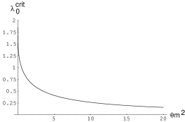
Figure 1: Critical eigenvalue $\lambda_{0}^{crit}$ as a function of $\theta m^{2}$.

Two important results are immediately obvious from the solution. First, as $\theta m^{2}\rightarrow\infty$ we see $\lambda_{n}^{crit}\rightarrow 0$, as we would expect from the interpretation that the eigenvalues decouple and must simply be positive “on their own”. Second, the critical eigenvalues aren’t real for $m^{2}<0$, so, as expected, there are no stable solutions unless there is a stable true vacuum.

We then consider the corrections $\Delta\lambda_{n}^{crit}$,

$$\Delta\lambda_{n}^{crit}=-2\theta a\left(\frac{\lambda_{n}^{crit}}{2(n+1)}\right)^{2}\left(c_{n+1}+\left(\frac{\lambda_{n+1}^{crit}}{2(n+2)}\right)^{2}\left(c_{n+2}+\cdots\right)\right).$$ (3.17)

Since we know $\lambda_{n}^{crit}\leq 2(n+1),$

$$|\Delta\lambda_{n}^{crit}| \leq |2\theta a(c_{n+1}+c_{n+2}+\cdots)|$$ (3.18)

$$\approx \left|\frac{2\theta a}{m^{2}}\left(V^{\prime}(c_{n+1})+V^{\prime}(c_{n+2})+\cdots\right)\right|$$ (3.19)

The convergence of Eq. (3.19) was proved by [5] so this correction is well-defined. In fact the corrections are very small in most circumstances.

4 General Stability Analysis

Naturally one wonders what general statements about a solution’s stability are possible without checking the eigenvalues numerically.

4.1 Stability of the Gaussian

Let us focus on the Gaussian case to begin with; this is the unique level-1 solution at $\theta=\infty$ which is stable with respect to angular fluctuations. The solution requires $(\epsilon\equiv 1/\theta m^{2})$

$$\lim_{\epsilon\rightarrow 0}c_{0} \rightarrow c,$$ (4.20)

$$\lim_{\epsilon\rightarrow 0}c_{n} \rightarrow 0$$ (4.21)

uniformly in $n$ for $n\geq 1$. Let us quickly review the procedure to construct solutions at finite $\theta$, given in [3]. The perturbed equation of motion is

$$(-\epsilon\partial^{2}+1)\phi=b\phi_{0}$$ (4.22)

for some scale parameter $b$. This can be solved in Fourier-space as

$${\tilde{\phi}}(k)=b\frac{{\tilde{\phi}}_{0}(k)}{1+\epsilon k^{2}}.$$ (4.23)

Using expressions for ${\tilde{\phi}}(k)$ in terms of Laguerre polynomials $L_{n}(x)$ we can then calculate the solution from

$$c_{n}(\epsilon)=b\int_{0}^{\infty}\frac{e^{-x}L_{n}(x)}{1+2\epsilon x}\ dx.$$ (4.24)

The normalization of $L_{n}(x)$ is such that $\int_{0}^{\infty}e^{-x}L_{n}(x)L_{m}(x)dx=\delta_{mn}$. We determine $b$ by matching boundary conditions in Eq. (4.20) and Eq. (4.21) to get

$$V^{\prime}(bF(\epsilon))=m^{2}b(F(\epsilon)-1),\hskip 36.135ptF(\epsilon)=\int_{0}^{\infty}\frac{e^{-x}}{1+2\epsilon x}\ dx.$$ (4.25)

As explained in more detail by [5] and [6], the soliton ceases to exist when there is no such $b$. Just as finding solutions to the equation of motion at $\theta=\infty$ meant finding the real roots of $V^{\prime}$, we can think of this as finding the real roots of

$$V^{\prime}_{eff}(bF(\epsilon))\equiv V^{\prime}(bF(\epsilon))-m^{2}b(F(\epsilon)-1).$$ (4.26)

At $\epsilon_{c}\equiv 1/(\theta m^{2})_{c}$ the solution must also satisfy $\partial V^{\prime}_{eff}/\partial b=0$ (see Figure 2, for example), so

$$V^{\prime\prime}(b_{c}F(\epsilon_{c}))=m^{2}\left(1-\frac{1}{F(\epsilon_{c})}\right).$$ (4.27)

Plugging this into our expression for $\lambda_{0}$ provides a simple answer for the eigenvalue at the last point of existence for the solution, completely independent of potential:

$$\lambda_{0}((\theta m^{2})_{c}) = \theta V^{\prime\prime}(c_{0}(\epsilon_{c}))+2$$ (4.28)

$$= (\theta m^{2})_{c}\left(1-\frac{1}{F(\epsilon_{c})}\right)+2$$ (4.29)

$$= \lambda_{0}^{crit}((\theta m^{2})_{c})$$ (4.30)

where we use the identity proved in the appendix.

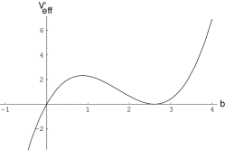
Figure 2: At $(\theta m^{2})_{c}$, $b$ will be a local minima of $V_{eff}$.

Then our Gaussian stability comes down to only determining the sign of $\Delta\lambda_{0}^{crit}$. If positive, it is slightly unstable; if negative, it is slightly stable. Examining the form of $\Delta\lambda_{0}^{crit}$ in Eq. (3.15) we see this is entirely determined by the sign of the $\phi^{3}$ coefficient $a/3$, since it was shown in [5][6] all $c_{n}>0$ if they come from $c_{n}=0$ at $\theta=\infty$.

We provide an example of this using the false-vacuum potential given by [5],

$$V(\phi)=3\phi^{2}-\frac{5}{3}\phi^{3}+\frac{1}{4}\phi^{4}.$$ (4.31)

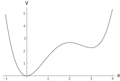
Figure 3: A typical false-vacuum potential.

This is graphed in Figure 3. Choose the solution $\phi=3\phi_{0}$ at $\theta=\infty$, so that we begin with a stable solution. It is easy to show that for this potential $(\theta m^{2})_{c}=46.1488$. From the procedure outlined this implies

$$\lambda_{0}((\theta m^{2})_{c}) = 0.0771,$$ (4.32)

$$\lambda_{0}^{crit}((\theta m^{2})_{c}) = 0.0771,$$ (4.33)

$$\Delta\lambda_{0}^{crit}((\theta m^{2})_{c}) = 0.0355.$$ (4.34)

In Figure 4 we plot $\lambda_{0}$ and $\lambda_{0}^{crit}$ near the critical point, seeing that indeed the solution has nearly neutral stability at its critical point. When we then consider the effect of raising the critical eigenvalue by $\Delta\lambda_{0}^{crit}((\theta m^{2})_{c})=0.0355$, we know it is unstable.

Figure 4: $\lambda_{0}$ and $\lambda_{0}^{crit}$ near the critical point.

4.2 Higher Levels

Let us now attempt to extend this to the level-$n$ solution,

$$\phi=c(\phi_{0}+\ldots+\phi_{n-1}).$$ (4.35)

Now $\phi(x)$ will obey

$$(-\epsilon\partial^{2}+1)\phi(x)=\sum_{j=0}^{n-1}b_{j}\phi_{j}(x)$$ (4.36)

and we can obtain coefficients from

$$c_{i}=\sum_{j=0}^{n-1}b_{j}F_{ij}(\epsilon)$$ (4.37)

where

$$F_{ij}(\epsilon)\equiv\int_{0}^{\infty}\frac{e^{-x}}{1+2\epsilon x}L_{i}(x)L_{j}(x)\ dx$$ (4.38)

which is clearly symmetric under $i\leftrightarrow j$. The equations of motion combined with boundary conditions are

$$\frac{1}{m^{2}}V^{\prime}(c_{i})=-b_{i}+\sum_{j=0}^{n-1}b_{j}F_{ij}.\hskip 36.135pt(i=0,\ldots,n-1)$$ (4.39)

Now rewrite this in the $\{c_{i}\}$ basis using the substitution

$$b_{i}={\bf F}_{ij}^{-1}c_{j}$$ (4.40)

where ${\bf F}_{ij}^{-1}$ is the matrix inverse of ${\bf F}_{ij}\equiv\{F_{ij}\}$. These equations then need to be decoupled to obtain solutions for each $c_{i}$. For $\theta=\infty$ this decoupling is trivial since $F_{ij}(\epsilon=0)=\delta_{ij}$, producing $V^{\prime}(c_{i})=0$ as expected. But at finite $\theta$ the equations will include terms such as $V^{\prime}(V^{\prime}(c_{i}))$ and be of higher order. This implies there will be an increase in the number of solutions. It is then potentially ambiguous how to extrapolate $\theta=\infty$ solutions into finite $\theta$, and thus it is unclear how one could single out the solution which remains at lowest $\theta$. To our knowledge, this solution ambiguity has not been discussed before.

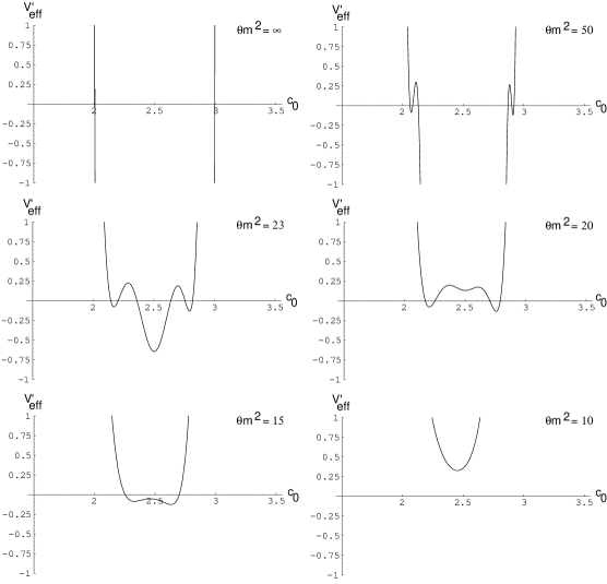
Figure 5: $V^{\prime}_{eff}(c_{0})$ at several values of $\theta m^{2}$.

Let us demonstrate this concept explicitly in a level-2 solution. Eq. (4.39) becomes

$$V^{\prime}(c_{0}) = b_{0}(F_{00}-1)+b_{1}F_{01},$$ (4.41)

$$V^{\prime}(c_{1}) = b_{0}F_{01}+b_{1}(F_{11}-1).$$ (4.42)

Changing basis allows us to write these as

$$V^{\prime}(c_{0}) = \alpha c_{0}+\beta c_{1},$$ (4.43)

$$V^{\prime}(c_{1}) = \beta c_{0}+\gamma c_{1}.$$ (4.44)

where

$$\alpha=\frac{1}{\Delta}(\Delta-F_{11}),\hskip 28.90755pt\beta=\frac{F_{01}}{\Delta},\hskip 28.90755pt\gamma=\frac{1}{\Delta}(\Delta-F_{00}),\hskip 28.90755pt\Delta\equiv F_{00}F_{11}-F_{01}^{2}.$$ (4.45)

These are easily decoupled to get

$$\frac{1}{m^{2}}V^{\prime}\left(\frac{1}{\beta}\left(V^{\prime}(c_{1})-\gamma c_{1}\right)\right) = \frac{\alpha}{\beta}\left(V^{\prime}(c_{1})-\gamma c_{1}\right)+\beta c_{1},$$ (4.46)

$$\frac{1}{m^{2}}V^{\prime}\left(\frac{1}{\beta}\left(V^{\prime}(c_{0})-\alpha c_{0}\right)\right) = \frac{\gamma}{\beta}\left(V^{\prime}(c_{0})-\alpha c_{0}\right)+\beta c_{0}.$$ (4.47)

We show in Figure 5 the solutions to Eq. (4.47) at various values of $\theta$, using the same false vacuum potential as we did in the Gaussian case. Multiple solutions are clearly evident at finite $\theta$, each of which has a different $(\theta m^{2})_{c}$.

5 Conclusion

We have presented the conditions by which radial stability of a noncommutative scalar soliton may be determined. One may explicitly calculate the stability eigenvalues of the solution and then compare these to critical eigenvalues which ensure the stability of the system. For a level-1 solution, we found that the existence and stability of a system are closely intertwined, allowing one to make definite statements about the stability of a system at its critical existence point. For level-$n$ solitons we do not believe such a general statement can be made, due to the nonuniqueness of solutions at finite $\theta$.

There are many possible extensions of the analysis presented here. The first would be a complete analysis of these extra level-$n$ solutions at finite $\theta$. Another would be a comparison with the work by Aganagic et al. [4] in which unstable solitons in noncommutative gauge theory were addressed. Also interesting would be to place this in the context of the large literature in which noncommutative methods have been applied to unstable D-branes and tachyonic condensation. Yet another is that our methods only address classical stability and it would be very interesting to include quantum stability.

6 Acknowledgements

The author thanks D. Tong, B. Greene, D. Goldfeld, R. Gopakumar, and H. Peiris for helpful comments. This work was supported by a GAANN Fellowship from the United States Department of Education.

7 Appendix: Equivalence of formulae

Here we present a proof for the equality of

$$x(1-1/F(x))+2=\lambda^{crit}_{0}(x)$$ (7.48)

where

$$F(x) = \int_{0}^{\infty}\frac{e^{-u}}{1+2u/x}\ du$$ (7.49)

$$= \frac{x}{2}e^{x/2}\Gamma(0,\frac{x}{2})$$ (7.50)

and

$$\lambda_{n}^{crit}(x)=\frac{(2(n+1))^{2}}{x+2(2n+3)-\lambda^{crit}_{n+1}(x)}.$$ (7.51)

We can re-write Eq. (7.48) as

$$x+1-\frac{\lambda^{crit}_{0}(2x)}{2} = \frac{x}{F(2x)}$$ (7.52)

$$x+1-\frac{1^{2}}{x+3-\frac{2^{2}}{x+5-\ldots}} = \frac{1}{e^{x}\ \Gamma(0,x)}$$ (7.53)

To prove this we use an identity found in Perron [8] §82 formula (26)

$$x+\alpha+\beta+1-\frac{(\alpha+1)(\beta+1)}{x+\alpha+\beta+3-\frac{(\alpha+2)(\beta+2)}{x+\alpha+\beta+5-\ldots}}=\frac{\beta\int_{0}^{\infty}\frac{e^{-u}u^{\beta-1}}{(x+u)^{\alpha}}\ du}{\int_{0}^{\infty}\frac{e^{-u}u^{\beta}}{(x+u)^{\alpha+1}}\ du}$$ (7.54)

which holds for $\beta\geq 0,\alpha\geq 0,x\geq 0$. We note that

$$\lim_{\beta\rightarrow 0}\beta\int_{0}^{\infty}e^{-u}u^{\beta-1}du = \lim_{\beta\rightarrow 0}\beta\ \Gamma(\beta)$$ (7.55)

$$= 1.$$ (7.56)

Using this we take the $\alpha=0,\beta\rightarrow 0$ limit of Eq. (7.54) to find

$$x+1-\frac{1^{2}}{x+3-\frac{2^{2}}{x+5-\ldots}} = \frac{1}{\int_{0}^{\infty}\frac{e^{-u}}{x+u}\ du}$$ (7.57)

$$= \frac{1}{e^{x}\ \Gamma(0,x)}.$$ (7.58)

We thank D. Goldfeld for providing us with this proof.

References

- [1] A. Connes, M. R. Douglas and A. Schwarz, “Noncommutative Geometry and Matrix Theory: Compactification on Tori,” JHEP 9802 (1998) 003, hep-th/9711162.
- [2] N. Seiberg and E. Witten, “String Theory and Noncommutative Geometry”, JHEP 9909 (1999) 032, hep-th/9908142.
- [3] R. Gopakumar, S. Minwalla and A. Strominger, “Noncommutative Solitons”, hep-th/0003160, JHEP 0005 (2000) 020.
- [4] M. Aganagic, R. Gopakumar, S. Minwalla, and A. Strominger, “Unstable Solitons in Noncommutative Gauge Theory”, hep-th/0009142.
- [5] C. Zhou, “Noncommutative Scalar Solitons at Finite ”, hep-th/0007255.
- [6] B. Durhuus, T. Jonsson, R. Nest, “Noncommutative Scalar Solitons: Existence and Nonexistence”, hep-th/0011139.
- [7] R. Gopakumar and M. Headrick, “Noncommutative Solitons I”, Presentation at Strings 2001.
- [8] O. Perron, Die Lehre von den Kettenbrüchen, Chelsea Publishing Company.