Coupled fields in external background
with application to non-thermal
production of gravitinos

Abstract:

We provide the formalism for the quantization of systems of coupled bosonic and fermionic fields in a time dependent classical background. The occupation numbers of the particle eigenstates can be clearly defined and computed, through a generalization of the standard procedure valid for a single field in which Bogolyubov coefficients are employed. We apply our formalism to the problem of non-thermal gravitino production in a two-fields model where supersymmetry is broken gravitationally in the vacuum. Our explicit calculations show that this production is strongly suppressed in the model considered, due to the weak coupling between the sector which drives inflation and the one responsible for supersymmetry breakdown.

1 Introduction

The analysis of quantized systems in a classical background can be very useful for the study of various phenomena that arise in quantum theories, as for example particle production. The study of matter in external electromagnetic fields [1] dates back to the first years of quantum field theory [2, 3]. For what concerns gravity [4], the semiclassical approximation is often compulsory, due to the lack of a consistent quantum theory. Despite of this, it turned out very successful in describing phenomena as particle creation from black holes [5] or the generation of the perturbations in the inflationary Universe [6].

In the last ten years, this semiclassical approach has been applied to non-thermal particle production after inflation. In this case, the classical background is given by the inflaton field, which is coherently oscillating about the minimum of its potential. The first analyses of this phenomenon were performed in [7], but its full relevance was appreciated only a few years later in the case of production of scalars [8, 9, 10]. In the work [8] this non-perturbative production has been called “preheating”, since it is usually followed by a ordinary phase of perturbative reheating. It has been there understood that preheating of bosons is characterized by a very efficient and explosive creation, even when single particle decay is kinematically forbidden. This is due to the coherent inflaton oscillations, which allow stimulated particle production into energy bands with very large occupation numbers.

Less attention was initially paid to non-perturbative production of fermions. Indeed, the efficiency of this process seems to be strongly limited by Pauli blocking, which does not allow for occupation numbers bigger than one. However, also this production turned out very relevant, as the first complete calculation [11] of the inflaton decay into heavy (spin $1/2$) fermions during preheating showed. Indeed, if one only considers the most natural interactions $\phi\,{\bar{\psi}}\,\psi$ and $\phi^{2}\,\chi^{2}$ of the inflaton $\phi$ to fermions $\psi$ or to bosons $\chi$, fermionic production occurs in a mass range much broader than the one for heavy bosons, and this can “compensate” the limit imposed by Pauli blocking [11].

These results were soon applied [14, 15] to non-thermal gravitino production, since the equations for the different components of the gravitino field can be reduced to the one of a spin $1/2$ particle. As had also been realized in [16], the transverse gravitino component is always very weakly coupled to the background and decoupled from the other fermions, so that the production of its quanta is negligible. However, the works [14, 15] also studied the production of the longitudinal component, concluding that it easily exceeds the limits imposed by primordial nucleosynthesis (the so called “gravitino problem” [17]). The analyses of [14, 15] were extended in [18, 19] and followed by several related works [20, 21].

Most of these analyses support the conclusions of [14, 15] of a gravitino overproduction at preheating. However, in all the explicit calculations, only the case of one chiral superfield with supersymmetry unbroken in the vacuum was considered. This last issue is however crucial to understand the gravitino production: in the super-higgs mechanism (in the unitary gauge), the gravitino longitudinal component is provided by the goldstino, which is present only when supersymmetry is broken. As pointed out in the works [18, 19], during the cosmological evolution supersymmetry is broken both by the kinetic and the potential energies of the scalar fields of the theory. However, these fields are expected to be settled in their minima now. If in these minima supersymmetry is unbroken the gravitino has only the transverse component and it is massless. The calculations performed in these schemes show that one fermionic component is produced at preheating. However, we have remarked that at late times it cannot be the longitudinal gravitino component. Since this fermion is the partner of the inflaton field (in case of only one chiral multiplet the scalar is necessarily the inflaton), it should be better denoted as “inflatino”. Since this field does not have a gravitational decay rate, we conclude that preheating does not contribute to the gravitino problem in models with supersymmetry unbroken in the vacuum.

One is thus led to consider schemes where both the issues of inflation at early times and supersymmetry breaking today are included. From COBE normalization of the scalar metric perturbation, the relevant scale of inflation (when only one field is present) is expected to be about $10^{13}\,\mathrm{GeV}$. Supersymmetry provides instead a solution to the hierarchy problem if it is broken at about the TeV scale. Although in principle one may construct a model where a unique field satisfies both these requirements, we do not consider this option as the most natural one. Moving to the two fields case, the simplest possibility is to consider two well separate sectors, one of which drives inflation, while the second is responsible for supersymmetry breaking today. We have in mind a situation in which no direct coupling is present between the two fields in the superpotential, so to have a strong suppression in the interactions between the inflaton and the field which provides the longitudinal gravitino component. As we describe below, with two chiral supermultiplets the longitudinal gravitino component is coupled to one other fermionic field (the matter component orthogonal to the goldstino). For simplicity, in the rest of the introduction we refer to these two fields simply as to the gravitino and to the inflatino, although this interpretation is true only in the vacuum of the theory and more rigorous definitions will be provided below. The coupled system is particularly involved, so that trying to guess its behavior without an explicit calculation results very difficult. One can guess that at the preheating era only the inflatino field is produced. However, there is the potential worry that much later (on a physical time-scale of the order the inverse gravitino mass, when supersymmetry is equally broken by the two sectors of the theory) a fraction of inflatinos is “converted” in gravitinos. As remarked in [19], this worry requires an explicit calculation in a full supergravity context.

The problem of gravitino production is thus reduced to the problem of a (quite involved) coupled system in the external background constituted by the scalar fields of the theory. The most difficult part of this analysis is to provide a formalism in which the coupled system is quantized, with a clear definition of the occupation numbers for the physical eigenstates. This is a very interesting problem in itself, which can have several other applications besides the one we will consider in the present paper. In the one field case, the procedure is well established [12, 22]. One first quantizes the system and expands the canonical hamiltonian in the creation and annihilation operators of the field. The evolution of the background creates a mixing between the positive and negative energy solutions of the field equation, which has the consequence of driving the hamiltonian non diagonal, even if one takes it to be diagonal at initial time. A diagonal form is achieved through a (time dependent) redefinition of the creation/annihilation of the fields. The two coefficients of this diagonalization are known as Bogolyubov coefficients and can be easily related to the occupation number for the quantized field (consistency of the quantization requires a relation between these coefficient; this condition is however preserved by the equations of motion of the system).

In the first part of the present work we generalize this procedure for systems of multi-fields, both in the bosonic and in the fermionic case. Although far from trivial, this generalization can be presented in a remarkably simple form. By choosing a suitable expansion of the fields we can repeat each step of the above analysis substituting the Bogolyubov coefficients with two matrices $\alpha$ and $\beta$ (the expansion is now performed in a basis of creation/annihilation operators, each corresponding to a physical eigenstate of the system after the diagonalization of the hamiltonian). We can obtain a system of first order differential equations for these matrices; the condition on $\alpha$ and $\beta$ for a consistent quantization are also very simple and are preserved by these equations. Finally, the expression for the occupation numbers is an easy generalization of the one valid in the one field case. This first part is divided in two sections, the first of which is devoted to bosons, while the second one to fermions. This second section is further divided in two parts. In the first one we consider the case in which the fermionic fields are coupled only through the “mass matrix”, while in the second one we consider a more general system which is necessary for the application to the gravitino case.

The second part of the work is completely devoted to this application. In section 4.1 we introduce the quantities relevant for the calculation, following the notation of [19]. In section 4.2 we describe the model we are considering, discussing the evolution of the scalar fields. In section 4.3 we write the effective lagrangian for the longitudinal gravitino component and the matter fermion in the two chiral supermultiplets case. In the last two subsections we present our results for the gravitino and the inflatino production. In section 4.4 we present analytical results for the case in which supersymmetry is unbroken in the vacuum, while numerical results for the case of broken supersymmetry are shown in section 4.5. As we will see, the final gravitino production is strongly sensitive to the size of the supersymmetry breaking: our numerical results indicate that this production goes to zero in the limit of a vanishing final supersymmetry breaking. This limit is in agreement with the analytical result of section 4.4 and with the fact that the longitudinal gravitino component is actually absent when supersymmetry is preserved. We thus conclude that in the model considered here, non-thermal gravitino production is strongly suppressed. This appears as the consequence of the weak coupling between the two sectors responsible for inflation and supersymmetry breakdown, and of the strong hierarchy between the two scales that characterize them.

A short description of our results for the gravitino and inflatino production can be found in [23].

2 System of coupled bosonic fields

In this section we consider the coupled system of $N$ bosonic fields $\{\phi_{i}\}$ in a FRW background described by the action

$$S=\frac{1}{2}\,\int d^{4}x\,\sqrt{-\,g}\Big{[}\partial_{\mu}\phi_{i}\,\partial^{\mu}\phi_{i}-m_{i\,j}^{2}\phi_{i}\,\phi_{j}+\xi\,R\,\phi_{i}\phi_{i}\Big{]}\,.$$ (1)

We use conformal time $\eta$, such that the metric and the Ricci scalar are $g_{\mu\,\nu}=a^{2}(\eta)\mathop{\rm diag}\nolimits(1,\,-1,\,-1,\,-1)$ and $R=-\,6\,\ddot{a}/a^{3}$, where $a$ is the scale factor of the Universe and dot denotes derivative with respect to $\eta$ (summation over repeated indices is understood). The last term describes a possible non-minimal coupling ($\xi\neq 0$) of the scalar fields to gravity.

The (symmetric) mass matrix $m_{i\,j}^{2}$ is assumed to be a function of some external (background) fields. The only assumption that we do on these external fields is that they are constant (or better, adiabatically evolving) at the very beginning and at the very end of the evolution of the system. In these regimes, the matrix $m_{i\,j}^{2}$ becomes also constant and the fields which diagonalize it become free fields, whose masses are precisely given by the eigenvalues of $m_{i\,j}^{2}$. However, during the evolution the different entries of $m_{i\,j}^{2}$ are allowed to vary, and the (time dependent) eigenvalues of $m_{ij}^{2}$ are interacting fields whose masses change in time. These masses can change non adiabatically and this may in general lead to particle production. The aim of this section is to give a precise definition of the occupation number and to provide the formalism to calculate it.

It is most convenient to consider the “comoving” fields $\varphi_{i}\equiv a\,\phi_{i}$. For these fields, the above action (1) rewrites

$$S = \frac{1}{2}\int d^{4}x\left[\dot{\varphi_{i}}\,\dot{\varphi_{i}}-\varphi_{i}\,\Omega_{ij}^{2}\,\varphi_{j}\right],$$

$$\Omega_{ij}^{2} \equiv a^{2}\,m_{ij}^{2}+\left(-\Delta+\frac{\ddot{a}}{a}\left(6\,\xi-1\right)\right)\delta_{ij}\,,$$ (2)

where $\Delta$ is the laplacian operator. We can also write the hamiltonian of the system, which, in terms of the fields $\varphi_{i}$ and their conjugate momenta

$$\Pi_{i}\equiv\frac{\partial\,\mathcal{L}}{\partial\dot{\varphi_{i}}}=\dot{\varphi_{i}}\,,$$ (3)

reads

$$H\equiv\int d^{3}\mathbf{x}\,\mathcal{H}=\frac{1}{2}\int d^{3}\mathbf{x}\left(\Pi_{i}\,\Pi_{i}+\varphi_{i}\,\Omega_{ij}^{2}\varphi_{j}\right).$$ (4)

The frequency matrix $\Omega_{ij}^{2}$ which enters in the above expressions is also in general time dependent and non diagonal. At any given time, it can be diagonalized with an orthogonal matrix $C$

$$C^{T}\left(\eta\right)\Omega^{2}\left(\eta\right)C\left(\eta\right)=\omega^{2}\left(\eta\right)\qquad\mbox{diagonal}\,.$$ (5)

We denote by ${\hat{\varphi}}\equiv C^{T}\,\varphi$ the bosonic fields in the basis in which the frequency matrix is diagonal. We also denote by $\omega_{i}^{2}$ the $i$-th entry of the diagonal matrix $\omega^{2}$. The set of $\omega_{i}$ represents the energy densities of the (time dependent) physical eigenstates of the system ${\hat{\varphi}_{i}}$.

We now show that the occupation numbers of these fields can be defined and computed generalizing the usual techniques based on Bogolyubov coefficients valid in the one field case. The first step to do this is to consider a basis for annihilation/creation operators $\{a_{i}\}$ and $\{a_{i}^{\dagger}\}$ and to perform the decompositions

$$\varphi_{i} = C_{ij}\int\frac{d^{3}k}{\left(2\,\pi\right)^{3/2}}\left[\mathrm{e}^{i\,\mathbf{k}\cdot\mathbf{x}}\,h_{jk}\left(\eta\right)a_{k}\left(k\right)+\mathrm{e}^{-i\,\mathbf{k}\cdot\mathbf{x}}\,h_{jk}^{*}\left(\eta\right)a_{k}^{\dagger}\left(k\right)\right],$$

$$\Pi_{i} = C_{ij}\int\frac{d^{3}k}{\left(2\,\pi\right)^{3/2}}\left[\mathrm{e}^{i\,\mathbf{k}\cdot\mathbf{x}}\,{\tilde{h}_{jk}}\left(\eta\right)a_{k}\left(k\right)+\mathrm{e}^{-i\,\mathbf{k}\cdot\mathbf{x}}\,{\tilde{h}_{jk}^{*}}\left(\eta\right)a_{k}^{\dagger}\left(k\right)\right].$$ (6)

The reason why we explicitly factorized the matrix $C$ in these decompositions will be clear soon. Due to the fact that the fields are coupled together, the matrices $h$ and ${\tilde{h}}$ are generically expected to be non diagonal.

To quantize the system, we impose

$$\left[\varphi_{i}\left(x\right),\,\Pi_{j}\left(y\right)\right]=i\,\delta^{3}\left(\mathbf{x}-\mathbf{y}\right)\delta_{ij}$$ (7)

for the conjugate fields, and

$$\left[a_{i}\left(\mathbf{k}\right),a_{j}^{\dagger}\left(\mathbf{p}\right)\right]=\delta^{3}\left(\mathbf{k}-\mathbf{p}\right)\delta_{ij}$$ (8)

for the annihilation/creation operators. We can satisfy both these relations requiring

$$\left[h\,{\tilde{h}^{\dagger}}-h^{*}\,{\tilde{h}}^{T}\right]_{ij}=i\,\delta_{ij}\,,$$ (9)

as it can be easily checked from the decomposition (6).

From the action (2), one deduces the second order equations of motion

$$\ddot{\varphi_{i}}+\Omega_{ij}^{2}\,\varphi_{j}=0\,.$$ (10)

However, one can achieve a system of only first order equations by setting some additional relations between the conjugate fields $\varphi_{i}$ and $\Pi_{i}$. We want these relations to generalize the one which is usually taken in the one field case, see i.e. [22]. Also we want them to allow a rewriting of the hamiltonian (4) in a simple and readable form. The sets of fields where this generalization is most evident is given by $\{{\hat{\varphi}_{i}},{\hat{\Pi}_{i}}\equiv(C^{T}\,\Pi)_{i}\}$. These fields are decomposed as in eqs. (6), only without the $C$ matrix before the integrals. In terms of these fields, the hamiltonian (4) rewrites

$$H=\int d^{3}\mathbf{x}\;\frac{1}{2}\left({\hat{\Pi}_{i}}\,{\hat{\Pi}_{i}}+\omega_{i}^{2}\,{\hat{\varphi}_{i}}\,{\hat{\varphi}_{i}}\right),$$ (11)

since the frequency $\omega$ is diagonal. One is thus led to impose the conditions

$$h = \frac{\mathrm{e}^{-i\,\int^{\eta}\omega\,d\eta^{\prime}}}{\sqrt{2\,\omega}}\,A+\frac{\mathrm{e}^{i\,\int^{\eta}\omega\,d\eta^{\prime}}}{\sqrt{2\,\omega}}\,B\,,$$

$${\tilde{h}} = \frac{-\,i\,\omega\,\mathrm{e}^{-i\,\int^{\eta}\omega\,d\eta^{\prime}}}{\sqrt{2\,\omega}}\,A+\frac{i\omega\,\mathrm{e}^{i\,\int^{\eta}\omega\,d\eta^{\prime}}}{\sqrt{2\,\omega}}\,B$$ (13)

which are indeed a natural generalization of the one which is usually taken in the one field case [22]. For one field, $A$ and $B$ are numbers, known as Bogolyubov coefficients. In our case they are $N\times N$ matrices. The analysis of the system is in our case simplified if we consider, rather then the matrices $A$ and $B$, the combinations

$$\alpha \equiv \mathrm{e}^{-i\,\int^{\eta}\omega\,d\eta^{\prime}}\,A\,,$$

$$\beta \equiv \mathrm{e}^{i\,\int^{\eta}\omega\,d\eta^{\prime}}\,B\,.$$ (14)

The above condition (9) is satisfied if the matrices $\alpha$ and $\beta$ obey the relations

$$\alpha\,\alpha^{\dagger}-\beta^{*}\,\beta^{T} = 1\,,$$

$$\alpha\,\beta^{\dagger}-\beta^{*}\,\alpha^{T} = 0\,.$$ (15)

These relations can be imposed at the initial time, and are preserved by the evolution, as we shortly discuss. In the one field case, they reduce to the usual condition $|\alpha|^{2}-|\beta|^{2}=|A|^{2}-|B|^{2}=1$.

As we have said, the evolution of the system can be described by two sets of first order differential equations. The first set is obtained by inserting eqs. (6) into the definition of the conjugate momenta, eq. (3)

$${\dot{h}}={\tilde{h}}-\Gamma\,h\,,$$ (16)

where we have defined the matrix

$$\Gamma=C^{T}\,\dot{C}\,,\qquad\Gamma^{T}=-\Gamma\,.$$ (17)

The second set of equations is obtained by rewriting eqs. (10) in terms of $\varphi_{i}$ and $\Pi_{i}$

$$\dot{\tilde{h}}=-\Gamma\,{\tilde{h}}-\omega^{2}\,h\,.$$ (18)

We can now use relations (13) and decouple the terms proportional to $\dot{\alpha}$ and $\dot{\beta}$, so to arrive to the final result

$$\dot{\alpha} = -i\,\omega\,\alpha+\frac{\dot{\omega}}{2\,\omega}\,\beta-I\,\alpha-J\,\beta\,,$$

$$\dot{\beta} = \frac{\dot{\omega}}{2\,\omega}\,\alpha+i\,\omega\,\beta-J\,\alpha-I\,\beta\,,$$ (19)

where we have defined the matrices

$$I = \frac{1}{2}\left(\sqrt{\omega}\,\Gamma\,\frac{1}{\sqrt{\omega}}+\frac{1}{\sqrt{\omega}}\,\Gamma\,\sqrt{\omega}\right),\qquad I^{T}=-I\,,$$

$$J = \frac{1}{2}\left(\sqrt{\omega}\,\Gamma\,\frac{1}{\sqrt{\omega}}-\frac{1}{\sqrt{\omega}}\,\Gamma\,\sqrt{\omega}\right),\qquad J^{T}=J\,.$$ (20)

In the one field case, $I=J=\Gamma=0$, and the above system reduces to the equations for the two Bogolyubov coefficients

$$\dot{A}=\frac{\dot{\omega}}{2\,\omega}\,\mathrm{e}^{2\,i\,\int^{\eta}\omega\,d\eta^{\prime}}B\,,\qquad\dot{B}=\frac{\dot{\omega}}{2\,\omega}\,\mathrm{e}^{-2\,i\,\int^{\eta}\omega\,d\eta^{\prime}}A\,,$$ (21)

already discussed in the previous literature (see i.e. [10]). In the one field case the only source of nonadiabaticity is related to a rapid change of the only frequency $\omega(\eta)$, so that the system is said to evolve adiabatically whenever the condition $\dot{\omega}\ll\omega^{2}$ is fulfilled. In the present case, there are more sources of nonadiabaticity, related to the fact that now the frequency $\Omega_{ij}$ is a $N\times N$ matrix. This is associated with the presence of non-vanishing matrices $I$ and $J$ in the equations of motion for the matrices $\alpha$ and $\beta$.

It is a straightforward exercise to show that the above equations (19) preserve the normalization conditions (15), due to the properties $I^{T}=-I$ and $J^{T}=J$.

In the one field case, the number of particles is given by the modulus square of the second Bogolyubov coefficient, $|B|^{2}$. We now show that also in the multi-field case it is generally related to the matrix $\beta$. To see this, we decompose also the energy density operator $\mathcal{H}$ (see eq. (4)) in the basis of annihilation and creation operators

$$\mathcal{H}=\left(a_{i}^{\dagger},\,a_{j}\right)\pmatrix{\mathcal{E}_{il}&\mathcal{F}_{jl}^{\dagger}\cr\mathcal{F}_{im}&\mathcal{E}_{jm}^{T}}\pmatrix{a_{l}\cr\ a_{m}^{\dagger}}.$$ (22)

From eqs. (6), one sees that the $N\times N$ matrices $\mathcal{E}$ and $\mathcal{F}$ which enter in this decomposition are given by

$$\mathcal{E} = \frac{1}{2}\left({\tilde{h}}^{\dagger}\,{\tilde{h}}+h^{\dagger}\,\omega^{2}\,h\right),$$

$$\mathcal{F} = \frac{1}{2}\left({\tilde{h}}^{T}\,{\tilde{h}}+h^{T}\,\omega^{2}\,h\right).$$ (23)

We can now generalize the procedure adopted in the one field case. The matrix that appears in eq. (22) can be put in diagonal form in a basis of new (time dependent) annihilation/creation operators. Only when the hamiltonian is diagonal, each pair of (redefined) operators can be associated to a physical particle, and used to compute the corresponding occupation number. The explicit computation gives

$$\mathcal{E} = \frac{1}{2}\left(\alpha^{\dagger}\,\omega\,\alpha+\beta^{\dagger}\,\omega\,\beta\right),$$

$$\mathcal{F} = \frac{1}{2}\left(\alpha^{T}\,\omega\,\beta+\beta^{T}\,\omega\,\alpha\right),$$ (24)

so that we found that expression (22) evaluates to

$$\mathcal{H}=\frac{1}{2}\left(a^{\dagger},\,a\right)\pmatrix{\alpha^{\dagger}&\beta^{\dagger}\cr\beta^{T}&\alpha^{T}}\pmatrix{\omega&0\cr 0&\omega}\pmatrix{\alpha&\beta^{*}\cr\beta&\alpha^{*}}\pmatrix{a\cr a^{\dagger}}.$$ (25)

In terms of the redefined annihilation/creation operators

$$\pmatrix{{\hat{a}}\cr{\hat{a}}^{\dagger}}\equiv\pmatrix{\alpha&\beta^{*}\cr\beta&\alpha^{*}}\pmatrix{a\cr a^{\dagger}}$$ (28)

the hamiltonian is thus diagonal (remember that in eq. (5) $\omega$ was defined to be diagonal), and, after normal ordering, it simply reads

$$H=\int d^{3}\,\mathbf{k}\>\omega_{i}\,{\hat{a}}_{i}^{\dagger}\,{\hat{a}}_{i}\,.$$ (29)

We choose at initial time $\alpha(\eta_{0})=\mathbbm{1},\ \beta(\eta_{0})=0$, so that conditions (15) are fulfilled. We also choose the initial state of the theory to be annihilated by the operators $a_{i}$. At any generic time, the occupation number of the $i$-th bosonic eigenstate is given by (notice that in this expression we do not sum over $i$)

$$N_{i}\left(\eta\right)=\langle{\hat{a}}_{i}^{\dagger}\,{\hat{a}}_{i}\rangle=\left(\beta^{*}\beta^{T}\right)_{ii}.$$ (30)

In the one field case the above relation reduces to the usual $N=|B|^{2}$. We see that our choices correspond to an initial vanishing occupation number for all the bosonic fields.

3 System of coupled fermionic fields

We now consider a system of coupled fermions. We divide this analysis in two subsections. The first of them extends to the fermionic case the results obtained for bosons in the previous section. Because of the repeated analogies, the discussion is here shorter than the above one, where more details can be found. In the second subsection we study a more general system of equations, which can be also relevant when the background is not constant. In particular, these can be important for cosmology, where the expansion of the Universe provides a preferred direction in time. In the next section we will indeed discuss non-perturbative production of gravitinos as an application of this analysis.

3.1 The simpler case

Let us consider the coupled system of $N$ fermionic fields $\{\psi_{i}\}$ in a FRW background described by the action

$$S=\int d^{4}x\,\sqrt{-g}\,{\bar{\psi}}_{i}\left[i\,\delta_{ij}\,\left({\tilde{\gamma}^{\mu}}\,\partial_{\mu}+\frac{3}{2}\,\frac{\dot{a}}{a}\,{\tilde{\gamma}^{0}}\right)-M_{ij}\right]\psi_{j}\,.$$ (31)

The gamma matrices ${\tilde{\gamma}^{\mu}}$ in FRW geometry are related to those ($\gamma^{\mu}$) in flat space by ${\tilde{\gamma}^{\mu}}=a^{-1}\,\gamma^{\mu}$, where $a\left(\eta\right)$ is the scale factor of the Universe. As before, conformal time $\eta$ is used, and the matrix $M_{ij}$ is considered to be a function of some external background fields. The requirement that the action is hermitean forces $M$ to be hermitean as well. For simplicity we will also take it to be real. We also require $M_{ij}$ to be constant (better, adiabatically evolving) at very early and late times, but we do not make any other assumption on its evolution.

After the redefinitions $X_{i}\equiv\psi_{i}\,a^{3/2}$, $m\equiv a\,M$, the action (31) reads

$$S=\int d^{4}x\,{\bar{X}}_{i}\left[i\,\delta_{ij}\,\gamma^{\mu}\,\partial_{\mu}-m_{ij}\right]X_{j}\,,$$ (32)

leading to the equations of motion (in matrix notation)

$$\left(i\,\gamma^{\mu}\,\partial_{\mu}-m\right)X=0\,.$$ (33)

The canonical hamiltonian is instead

$$H\equiv\int d^{3}\mathbf{x}\;\mathcal{H}=\int d^{3}\mathbf{x}\,{\bar{X}}\left[-i\,\gamma^{i}\,\partial_{i}+m\right]X\,.$$ (34)

In analogy with the bosonic case, we expand the fermionic eigenstates into a basis of creation/annihilation operators

$$X_{i}\left(x\right)=C_{ij}\int\frac{d^{3}\mathbf{x}}{\left(2\pi\right)^{3/2}}e^{i\mathbf{k\cdot x}}\Big{[}U_{r}^{jk}\left(k,\,\eta\right)a_{r}^{k}\left(k\right)+V_{r}^{jk}\left(k,\,\eta\right)b_{r}^{+k}\left(-k\right)\Big{]}\,,$$ (35)

where the matrix $C$ is employed into the diagonalization of the mass matrix $m$

$$\mu\equiv C^{T}\,m\,C\,,\qquad C\ \mbox{orthogonal}\,.$$ (36)

We also define the matrix (dot denotes derivative with respect to $\eta$)

$$\Gamma\equiv C^{T}\,\dot{C}\,,\qquad\Gamma^{T}=-\Gamma\,,$$ (37)

and the “generalized spinors”

$$U_{r}^{ij}\equiv\left[\frac{U_{+}^{ij}}{\sqrt{2}}\,\psi_{r},r\,\frac{U_{-}^{ij}}{\sqrt{2}}\,\psi_{r}\right]^{T},\qquad V_{r}^{ij}\equiv\left[\frac{V_{+}^{ij}}{\sqrt{2}}\,\psi_{r},r\,\frac{V_{-}^{ij}}{\sqrt{2}}\,\psi_{r}\right]^{T}$$ (38)

with $\psi_{+}=$ $\pmatrix{1\cr 0}$ and $\psi_{-}=$ $\pmatrix{0\cr 1}$ eigenvectors of the helicity operator $\mathbf{\sigma}\cdot\mathbf{v}/|\mathbf{v}|$.

Let us consider a set of fields $X_{i}$ which satisfy the above equations (33). Due to the fact that the matrix $m_{ij}$ is real and symmetric, then also the fields $X_{i}^{C}\equiv{\tilde{C}}\,{\bar{X}_{i}}^{T}$ (where ${\tilde{C}}$ is the charge conjugation matrix) are solutions of (33). As a consequence, one can impose the relation $U_{r}(k)={\tilde{C}}\,{\bar{V}}_{r}^{T}\,(-k)$, or, using eqs. (38),

$$V_{+}=-U_{-}^{*}\,,\qquad V_{-}=U_{+}^{*}\,.$$ (40)

Doing so, we have only to deal with the $U_{\pm}$ matrices. Taking the momentum $k$ along the third axis, their equations of motion read

$$\dot{U_{\pm}}=-i\,k\,U_{\mp}\mp i\,\mu\,U_{\pm}-\Gamma\,U_{\pm}\,.$$ (41)

The quantization of the system requires

$$\left\{X_{i}\left(\eta,\,\mathbf{x}\right),X_{j}^{\dagger}\left(\eta,\,\mathbf{y}\right)\right\} = \delta^{(3)}\left(\mathbf{x}-\mathbf{y}\right)\delta_{ij}\,,$$

$$\left\{a_{r\,i}\left(\mathbf{k}\right),\,a_{s\,j}^{\dagger}\left(\mathbf{p}\right)\right\} = \delta^{(3)}\left(\mathbf{k}-\mathbf{p}\right)\delta_{rs}\,\delta_{ij}\,,$$

$$\left\{b_{r\,i}\left(\mathbf{k}\right),\,b_{s\,j}^{\dagger}\left(\mathbf{p}\right)\right\} = \delta^{(3)}\left(\mathbf{k}-\mathbf{p}\right)\delta_{rs}\,\delta_{ij}\,.$$ (42)

We can simultaneously satisfy these conditions by setting

$$U_{+}U_{+}^{\dagger}+U_{-}^{*}\,U_{-}^{T} = 2\,\mathbbm{1}\,,$$

$$U_{+}\,U_{-}^{\dagger} = U_{-}^{*}\,U_{+}^{T}\,.$$ (43)

These conditions can be imposed at initial time, and are preserved by the evolution of the system (as it is easily checked from eqs. (41)).

We define the diagonal matrix

$$\omega=\sqrt{k^{2}+\mu^{2}}\,,$$ (44)

and we further expand

$$U_{+} \equiv \left(1+\frac{\mu}{\omega}\right)^{1/2}\mathrm{e}^{-i\int^{\eta}\omega\,d\eta^{\prime}}\,A-\left(1-\frac{\mu}{\omega}\right)^{1/2}\mathrm{e}^{i\int^{\eta}\omega\,d\eta^{\prime}}\,B$$

$$\equiv \left(1+\frac{\mu}{\omega}\right)^{1/2}\alpha-\left(1-\frac{\mu}{\omega}\right)^{1/2}\beta\,,$$

$$U_{-} \equiv \left(1-\frac{\mu}{\omega}\right)^{1/2}\mathrm{e}^{-i\int^{\eta}\omega\,d\eta^{\prime}}\,A+\left(1+\frac{\mu}{\omega}\right)^{1/2}\mathrm{e}^{i\int^{\eta}\omega\,d\eta^{\prime}}\,B$$ (45)

$$\equiv \left(1-\frac{\mu}{\omega}\right)^{1/2}\alpha+\left(1+\frac{\mu}{\omega}\right)^{1/2}\beta\,,$$

so that the above conditions (43) are satisfied if the matrices $\alpha$ and $\beta$ obey the relations

$$\alpha\,\alpha^{\dagger}+\beta^{*}\,\beta^{T} = \mathbbm{1}\,,$$

$$\alpha\,\beta^{\dagger}-\beta^{*}\,\alpha^{T} = 0\,.$$ (46)

In the one field case, $A$ and $B$ are numbers, known as Bogolyubov coefficients. In our case they are $N\times N$ matrices. The matrices $\alpha$ and $\beta$ are introduced since their equations of motion assume a simpler form then the corresponding ones for $A$ and $B$. In the one field case, the above relations (46) reduce to the usual condition $|A|^{2}+|B|^{2}=1$.

For fermions, the evolution equations for the matrices $\alpha$ and $\beta$ can be obtained in a more straightforward way with respect to the bosonic case. This is because eqs. (41) are already two sets of first order differential equations. Using the above decomposition (45), after some algebra we arrive to the final expressions

$$\dot{\alpha} = \left[-i\,\omega-I\right]\alpha+\left[-\frac{\dot{\mu}\,k}{2\,\omega^{2}}+J\right]\beta\,,$$

$$\dot{\beta} = \left[\frac{\dot{\mu}\,k}{2\,\omega^{2}}-J\right]\alpha+\left[i\,\omega-I\right]\beta\,,$$ (48)

where we have defined the matrices

$$2I \equiv \left(1+\frac{\mu}{\omega}\right)^{1/2}\Gamma\left(1+\frac{\mu}{\omega}\right)^{1/2}+\left(1-\frac{\mu}{\omega}\right)^{1/2}\Gamma\left(1-\frac{\mu}{\omega}\right)^{1/2},\qquad I^{T}=-I\,,$$

$$2J \equiv \left(1+\frac{\mu}{\omega}\right)^{1/2}\Gamma\left(1-\frac{\mu}{\omega}\right)^{1/2}-\left(1-\frac{\mu}{\omega}\right)^{1/2}\Gamma\left(1+\frac{\mu}{\omega}\right)^{1/2},\qquad J^{T}=J\,.\quad$$ (49)

One can easily verify that these equations preserve the above conditions (46).

To properly define and compute the occupation number for the fermionic eigenstates, as before we expand the energy density operator $\mathcal{H}$ (eq. (34)) in the basis of annihilation and creation operators

$$\mathcal{H}=\left(a_{i}^{\dagger}\,,\,b_{j}\right)\pmatrix{\mathcal{E}_{il}&\mathcal{F}_{jl}^{\dagger}\cr\mathcal{F}_{im}&-\mathcal{E}_{jm}^{T}}\pmatrix{a_{l}\cr b_{m}^{\dagger}}.$$ (50)

Using eqs. (35) and (38), we find

$$\mathcal{E}\left(\eta\right) \equiv \frac{1}{2}\Big{[}U_{+}^{+}\,\mu\,U_{+}-U_{-}^{+}\,\mu\,U_{-}+U_{+}^{+}\,k\,U_{-}+U_{+}^{+}\,k\,U_{+}\Big{]}\,,$$

$$\mathcal{F}\left(\eta\right) \equiv \frac{1}{2}\Big{[}-U_{+}^{T}\,\mu\,U_{-}-U_{-}^{T}\,\mu\,U_{+}+U_{+}^{T}\,k\,U_{+}-U_{-}^{T}\,k\,U_{-}\Big{]}\,,$$ (51)

while eqs. (45) lead to

$$\mathcal{E} = \alpha^{\dagger}\,\omega\,\alpha-\beta^{\dagger}\,\omega\,\beta\,,$$

$$\mathcal{F} = -\alpha^{T}\,\omega\,\beta-\beta^{T}\,\omega\,\alpha\,.$$ (52)

We have thus

$$\mathcal{H}=\left(a^{\dagger},\,b\right)\pmatrix{\alpha^{\dagger}&\beta^{\dagger}\cr-\beta^{T}&\alpha^{T}}\pmatrix{\omega&0\cr 0&-\omega}\pmatrix{\alpha&-\beta^{*}\cr\beta&\alpha^{*}}\pmatrix{a\cr b^{\dagger}}.$$ (53)

In terms of the redefined annihilation/creation operators

$$\pmatrix{{\hat{a}}\cr{\hat{b}}^{\dagger}}\equiv\pmatrix{\alpha&-\beta^{*}\cr\beta&\alpha^{*}}\pmatrix{a\cr b^{\dagger}}$$ (56)

the hamiltonian is thus diagonal, and, after normal ordering, it simply reads

$$H=\int d^{3}\,\mathbf{k}\>\omega_{i}\left({\hat{a}}_{i}^{\dagger}\,{\hat{a}}_{i}+{\hat{b}}_{i}^{\dagger}\,{\hat{b}}_{i}\right).$$ (57)

We choose at initial time $\alpha(\eta_{0})=1,\beta(\eta_{0})=0$, so that conditions (46) are fulfilled. We also choose the vacuum state of the theory to be annihilated by the initial annihilation operators $a_{i}$ and $b_{i}$. At any given time, the occupation number of the $i$-th fermionic eigenstate is given by (notice that in this expression we do not sum over $i$)

$$N_{i}\left(\eta\right)=\langle{\hat{a}}_{i}^{\dagger}\,{\hat{a}}_{i}\rangle=\langle{\hat{b}}_{i}^{\dagger}\,{\hat{b}}_{i}\rangle=\left(\beta^{*}\beta^{T}\right)_{ii}.$$ (58)

In the one field case the above relation reduces to the usual $N=|B|^{2}$. We see that our choices correspond to an initial vanishing occupation number for all the fermionic fields. Notice that particles and antiparticles have the same energy and are produced with the same amount, due to the reality conditions that we have imposed on the system. Finally, we observe that the first of conditions (46) guarantees that Pauli blocking is always satisfied.

3.2 A more general case

We now consider a more general action for the coupled system of $N$ fermionic fields. For future convenience, here we switch to the signature $-,+,+,+$ for the Minkowski metric, and we then work with the gamma matrices

$$\bar{\gamma}^{0}=\pmatrix{-i\,\mathbbm{1}&0\cr 0&i\,\mathbbm{1}},\qquad\bar{\gamma}^{i}=\pmatrix{0&-i\,\sigma_{i}\cr i\,\sigma_{i}&0}$$ (59)

in flat space.

By a suitable conformal rescaling of the fermionic fields and of their masses as we did before eq. (32), we can again remove the scale factor of the Universe from the kinetic term for the fermions. However, we are now interested in a more generic system, so that we consider, instead of (32), the action

$$S=\int d^{4}x\,{\bar{X}}_{m}\left[\bar{\gamma}^{0}\partial_{0}+\bar{\gamma}^{i}\,N\,\partial_{i}+M\right]_{mn}X_{n}\,,$$ (60)

where $N$ and $M$ are two $N\times N$ matrices of the form

$$N\equiv N_{1}+\bar{\gamma}^{0}\,N_{2}\,,\qquad M\equiv M_{1}+\bar{\gamma}^{0}\,M_{2}\,.$$ (61)

The matrices $N$ and $M$ are assumed to be functions of some external fields. We consider a situation in which these fields evolve in time. This time dependence justifies the general form for the action that we want to discuss. As we will see in the next section, this analysis can have relevance for cosmology, where the expansion of the Universe provides a natural direction for time. However, the system (60) could also arise in flat space from some general interactions between the fermions $X_{i}$ and other fields which have been integrated out. As in the previous analyses, our main goal is to discuss the definition of the occupation number of the physical eigenstates of the system, and to provide the formalism to calculate it.

We list here our assumptions on the matrices $M$ and $N$. First, we require them to change adiabatically at initial times, so to consistently define the initial occupation numbers. Then, we assume $M_{1}\rightarrow\mbox{constant},M_{2}\rightarrow 0,N\rightarrow\mathbbm{1}$ at late times, so to recover a system of “standard” decoupled particles at the end (indeed, one can choose the basis of fields $X_{i}$ such that the matrix $M$ is diagonal at the end). The requirement of an hermitean action translates into the conditions

$$N_{i}^{\dagger}=N_{i}\,,\qquad M_{1}=M_{1}^{\dagger}\,,\qquad M_{2}=-M_{2}^{\dagger}\,.$$ (62)

For simplicity, we will only consider real matrices, so that $N_{1}$, $N_{2}$ and $M_{1}$ are required to be symmetric, while $M_{2}$ antisymmetric. Finally, we impose an additional condition, which is that the kinetic term for the fermions “squares” to the D’Alambertian operator $\Box$. If we take the equations of motion following from (60),

$$\left[\bar{\gamma}^{0}\partial_{0}+\bar{\gamma}^{i}\,N\,\partial_{i}+M\right]X=0\,,$$ (63)

and we multiply them on the left by $[\bar{\gamma}^{0}\partial_{0}+\bar{\gamma}^{i}\,N\,\partial_{i}+M]^{\dagger}$, we get

$$\Big{\{}\partial_{0}^{2}-N^{\dagger}\,N\,\partial_{i}^{2}+M^{\dagger}\,M-\bar{\gamma}^{0}\left[\left(\partial_{0}N\right)\bar{\gamma}^{i}\,\partial_{i}+\left(\partial_{0}M\right)\right]\Big{\}}X=0\,.$$ (64)

We thus require $N^{\dagger}\,N\equiv\mathbbm{1}$. This rewrites on the conditions

$$N_{1}^{2}+N_{2}^{2}=\mathbbm{1}\,,\qquad\left[N_{1},\,N_{2}\right]=0\,.$$ (65)

Our strategy is to reduce this problem to the one we have already discussed. That is, we perform some redefinitions of the fields to put the action (60) into the form (32), where we perform the canonical quantization of the system in the way described in the previous subsection. The first of these redefinitions strongly relies on the above conditions (65). If $N$ is a unitary matrix, we can find a hermitean matrix $\Phi$ such that

$$N=\exp\left(2\,\Phi\,\bar{\gamma}^{0}\right),\qquad\Phi^{\dagger}=\Phi\,.$$ (66)

Due to the properties of the $\bar{\gamma}^{0}$ matrix, this amounts to

$$\cos\left(2\,\Phi\right)=N_{1}\,,\qquad\sin\left(2\,\Phi\right)=N_{2}\,.$$ (67)

After the redefinition $X\equiv\exp(-\bar{\gamma}^{0}\,\Phi){\hat{X}}$, the equations of motions (63) acquire the form

$$\left(\bar{\gamma}^{0}\,\partial_{0}+i\,\bar{\gamma}^{i}\,k_{i}+{\hat{M}}\right){\hat{X}}=0\,,$$ (68)

where we have expanded the fermions into plane waves $X_{i}(\eta,\,\mathbf{k})=\mathrm{e}^{i\,\mathbf{k\cdot x}}\,X_{i}(\eta)$ and introduced the new “mass matrix”

$${\hat{M}} = \exp\left(\bar{\gamma}^{0}\,\Phi\right)\left[M+\bar{\gamma}^{0}\partial_{0}\right]\exp\left(-\bar{\gamma}^{0}\,\Phi\right)$$ (69)

$$\equiv {\hat{M}}_{1}+\bar{\gamma}^{0}\,{\hat{M}}_{2}\,.$$

Notice that the two matrices ${\hat{M}}_{1}$ and ${\hat{M}}_{2}$ are symmetric and antisymmetric, respectively. This means that, in the one field case, one recovers the standard equation

$$\left(\bar{\gamma}^{0}\,\partial_{0}+i\,\bar{\gamma}^{i}\,k_{i}+m\right){\hat{\theta}}=0$$ (70)

for spin $1/2$ fermions.

We have instead to perform a further redefinition of the fields. Setting ${\hat{X}}=L\,\Xi$, we have

$$L^{T}\left[L\left(\bar{\gamma}^{0}\,\partial_{0}+i\,\bar{\gamma}^{i}\,k_{i}\right)+{\hat{M}}_{1}\,L+\bar{\gamma}^{0}\left(\partial_{0}+{\hat{M}}_{2}\right)L\right]\Xi=0\,.$$ (72)

The matrix $L$ can be chosen such that $(\partial_{0}+{\hat{M}}_{2})L=0$. In particular, since ${\hat{M}}_{2}$ is antisymmetric and real, $L$ can be taken orthogonal. The equations of motion for the fields $\Xi$ can be thus cast in the form

$$\left(\bar{\gamma}^{0}\,\partial_{0}+i\,\bar{\gamma}^{i}\,k_{i}+L^{T}\,{\hat{M}_{1}}\,L\right)\Xi=0\,,$$ (73)

that is with the identity matrix multiplying the term which depends on the momentum and without any $\bar{\gamma}^{0}$ dependence in the “mass” matrix.

These equations (and the respective action for the fields $\Xi_{i}$) are exactly of the form considered in the previous subsection, so that we can apply the quantization procedure discussed there. As before, the procedure is to canonically define the hamiltonian starting from the set of fields $\Xi$ and to expand it in a basis of creation/annihilation operators. The occupation numbers are then calculated after the diagonalization of the hamiltonian. It is possible to show that this procedure can be carried out starting from any of the basis for the fermionic fields, once the hamiltonian has been canonically defined in the basis $\Xi$. One can indeed explicitly verify that these calculations lead to the same results for the occupation numbers of the physical eigenstates, in the same way as in the bosonic case the result (23) can be computed starting from each of expressions (4) or (11).

We thus have

$$H \equiv {\bar{\Xi}}\left[i\,\bar{\gamma}^{i}\,k_{i}+L^{T}\,{\hat{M}_{1}}\,L\right]\Xi={\bar{\hat{X}}}\left[i\,\bar{\gamma}^{i}\,k_{i}+{\hat{M}_{1}}\right]{\hat{X}}$$ (74)

$$= {\bar{X}}\left[i\,\bar{\gamma}^{i}\,k_{i}\,\mathrm{e}^{2\,\bar{\gamma}^{0}\,\Phi}+\mathrm{e}^{-\,\bar{\gamma}^{0}\,\Phi}\,{\hat{M}}_{1}\,\mathrm{e}^{\bar{\gamma}^{0}\,\Phi}\right]X\,,$$

depending on which basis we work. In particular, when working with the ${\hat{X}_{i}}$ or the $X_{i}$ fields, the explicit knowledge of the matrix $L$ is not needed. We present here the computation in the initial basis $X_{i}$, which we found more convenient (in the numerical calculations) for the application that we present in the next section. In this basis, the hamiltonian (74) has the form

$$H={\bar{X}}\left[i\,\bar{\gamma}^{i}\,k_{i}N+{\tilde{M}}_{1}+\bar{\gamma}^{0}\,{\tilde{M}}_{2}\right]X\,,$$ (75)

where the matrices ${\tilde{M}}_{1}$ and ${\tilde{M}}_{2}$ can be obtained from eqs. (74) and (69). At the end of the evolution, we simply have ${\tilde{M}}_{1}+\bar{\gamma}^{0}\,{\tilde{M}}_{2}=M_{1}$ diagonal, so that one recovers the “standard” hamiltonian for a system of $N$ decoupled fermions whose masses coincide with the ones of the equations of motion (which also become “standard”).

To analyze the system during the evolution, we instead decompose the spinors $X_{i}$ as in eqs. (35) and (38). Taking the third coordinate along the momentum $k$, the equations of motion (63) rewrite:

$$\dot{U}_{\pm}=\mp\,i\left(M_{1}\mp\,i\,M_{2}\right)U_{\pm}-i\,k\,\left(N_{1}\pm\,i\,N_{2}\right)U_{\mp}\,.$$ (77)

It is straightforward to check that they preserve the conditions

$$U_{+}\,U_{+}^{\dagger}+U_{-}^{*}\,U_{-}^{T}=2\cdot\mathbbm{1}\,,\qquad U_{+}\,U_{-}^{+}=U_{-}^{*}\,U_{+}^{T}\,,$$ (78)

which ensure the consistency of the canonical quantization.

We then expand the hamiltonian formally as in eq. (50), where now the $\mathcal{E}$ and $\mathcal{F}$ matrices read

$$\mathcal{E} = U_{+}^{\dagger}\,k\left[N_{1}+i\,N_{2}\right]U_{-}+U_{-}^{\dagger}\,k\left[N_{1}-i\,N_{2}\right]U_{+}+$$

$$+\,U_{+}^{\dagger}\left[{\tilde{M}}_{1}-i\,{\tilde{M}}_{2}\right]U_{+}+U_{-}^{\dagger}\left[-{\tilde{M}}_{1}-i\,{\tilde{M}}_{2}\right]U_{-},$$

$$\mathcal{F} = U_{+}^{T}\,k\left[-N_{2}-i\,N_{1}\right]U_{+}+U_{-}^{T}\,k\left[-N_{2}+i\,N_{1}\right]U_{-}+$$ (79)

$$+\,U_{+}^{T}\left[-{\tilde{M}}_{2}+i\,{\tilde{M}}_{1}\right]U_{-}+U_{-}^{T}\left[-{\tilde{M}}_{2}+i\,{\tilde{M}}_{1}\right]U_{+}\,.$$

We notice the properties

$$\mathcal{E}^{\dagger}=\mathcal{E}\,,\qquad\mathcal{F}^{T}=\mathcal{F}\,.$$ (80)

The matrix entering in eq. (50) can be diagonalized through a unitary matrix $C$

$$C\;\overline{H}\left(k,\eta\right)C^{\dagger}=H_{d}\left(k,\eta\right)\qquad\mbox{diagonal}\,,$$ (81)

such that the energy density is

$$\mathcal{H}=\left(a^{+},b\right)\overline{H}\pmatrix{a\cr b^{\dagger}}\equiv\left({\hat{a}}^{+},{\hat{b}}\right)H_{d}\pmatrix{{\hat{a}}\cr{\hat{b}}^{\dagger}}.$$ (82)

A first step in this diagonalization can be made by noticing that the matrix $\overline{H}$ can be rewritten as

$$\overline{H}=\mathcal{U}^{\dagger}\>\overline{H}_{0}\>\mathcal{U}\,,$$ (83)

with

$$\overline{H}_{0}\equiv\pmatrix{-{\tilde{M}}_{1}+i\,{\tilde{M}}_{2}&k\,N_{1}+i\,k\,N_{2}\cr k\,N_{1}-i\,k\,N_{2}&{\tilde{M}}_{1}+i\,{\tilde{M}}_{2}}$$ (84)

hermitean and

$$\mathcal{U}\equiv\frac{1}{\sqrt{2}}\pmatrix{U_{+}&-i\,U_{-}^{*}\cr-U_{-}&-i\,U_{+}^{*}}$$ (85)

unitary, as it follows from eqs. (78).

We are not able to provide general analytical formulae for the diagonalization of the remaining matrix $\overline{H}_{0}$. This diagonalization can however be performed numerically. In addition, some important conclusions can be drawn from the properties of the matrix $\mathcal{H}$. Due to the relations (80), one can show (i.e. by counting the number of independent equations that must be satisfied) that the matrix $C$ entering in eq. (81) can be of the form

$$C\equiv\pmatrix{I&J\cr i\,J^{*}&-i\,I^{*}}$$ (86)

(where $I$ and $J$ are $N\times N$ matrices). Unitarity of $C$ requires

$$I\,I^{\dagger}+J\,J^{\dagger}=\mathbbm{1}\,,\qquad I^{\dagger}\,J=J^{T}\,I^{*}\,.$$ (87)

By explicitly performing the product (81) one realizes that the eigenvalues of the hamiltonian occur in pairs, and that $H_{d}$ is of the form
$\mathop{\rm diag}\nolimits(\omega_{1},\,\omega_{2},\,\dots,\,\omega_{N},-\omega_{1},-\omega_{2},\,\dots\,,-\omega_{N})$. The eigenstates corresponding to each couple $\pm\,\omega_{i}$ are to be interpreted as particle and antiparticle states with the same energy. Finally, it is possible to show that particles and antiparticles are produced in the same amount. Defining the vacuum state to be annihilated by the initial annihilation operators $a_{i}$ and $b_{i}$, we have indeed (we remind that in this expression we do not sum over $i$)

$$N_{i}\left(\eta\right)=\langle{\hat{a}}_{i}^{\dagger}\,{\hat{a}}_{i}\rangle=\langle{\hat{b}}_{i}^{\dagger}\,{\hat{b}}_{i}\rangle=\left(J\,J^{\dagger}\right)_{ii}.$$ (88)

We assume that no fermionic particles are present at initial time $\overline{\eta}$. In our formalism, this is equivalent to requiring $J(\overline{\eta})=0$. Notice also that the unitarity condition (87) ensures that the Pauli principle is always fulfilled.

4 One application: non-thermal gravitino production

In this section we discuss one application of the above formalism, i.e. non-thermal gravitino production in a system with two chiral superfields. This model consists of two chiral multiplets coupled only gravitationally. The scalar of the first multiplet is responsible for driving inflation, while the one of the second breaks supersymmetry in the vacuum. The motivations for this analysis, as well for the specific model chosen, are explained in the introduction (see also [23]).

This section is divided in five subsections. In the first one we introduce all the quantities relevant for this calculation. Although we have exactly followed the conventions of ref. [19], the aim of section 4.1 is to provide a practical self contained presentation. In section 4.2 we describe the model that we are considering. We also discuss there the evolution of the scalar fields, which constitute the external background for the fermionic fields. In section 4.3 we show how to apply the formalism of the previous section to the calculation of the abundances of the fermions of the theory. Our results are presented in the two remaining subsections. In section 4.4 we present analytical results in the case in which supersymmetry is actually unbroken in the vacuum of the theory. We show that in this case, gravitinos are only gravitationally (hence negligibly) produced. Already this consideration suggests that in the class of models we are considering (i.e. with the two sectors coupled only gravitationally) non-thermal gravitino production may be very inefficient in the realistic situation in which the observable supersymmetry breaking (TeV scale) is much smaller than the scale of inflation ($10^{13}\mathrm{GeV}$). This is confirmed by the numerical results presented in section 4.5, which show that gravitino production indeed decreases as the size of supersymmetry breakdown becomes smaller.

4.1 Definitions

We write here the relevant equations of motion for the gravitino field and the fermionic particles to which it is coupled. We follow the conventions of ref. [19]. The starting action is the one of $D=4,N=1$ supergravity, with four fermion interactions omitted. For simplicity, we do not consider any gauge multiplet, but for the moment we allow chiral superfields to be complex. The lagrangian reads

$$e^{-1}\mathcal{L} = -\frac{1}{2}\,M_{\mathrm{P}}^{2}\,R-g_{i}{}^{j}\left(\partial_{\mu}\,\phi^{i}\right)\left(\partial^{\mu}\phi_{j}\right)-V-$$ (89)

$$-\,\frac{1}{2}\,M_{\mathrm{P}}^{2}\,\bar{\psi}_{\mu}\,R^{\mu}+\frac{1}{2}\,m\,\bar{\psi}_{\mu R}\,\gamma^{\mu\nu}\,\psi_{\nu R}+\frac{1}{2}\,m^{*}\,\bar{\psi}_{\mu L}\,\gamma^{\mu\nu}\,\psi_{\nu L}-$$

$$-\,g_{i}{}^{j}\left[\bar{\chi}_{j}\,D\hskip-7.0pt/\hskip 3.0pt\chi^{i}+\bar{\chi}^{i}D\hskip-7.0pt/\hskip 3.0pt\chi_{j}\right]-m^{ij}\,\bar{\chi}_{i}\,\chi_{j}-m_{ij}\,\bar{\chi}^{i}\,\chi^{j}+$$

$$+\,\Big{(}2\,g_{j}{}^{i}\bar{\psi}_{\mu R}\,\gamma^{\nu\mu}\,\chi^{j}\,\partial_{\nu}\phi_{i}+\bar{\psi}_{R}\cdot\gamma\upsilon_{L}+\mbox{h.c.}\Big{)}\,.$$

The first line of eq. (89) concerns the scalar fields. The first term is the standard one of Einstein gravity, with $M_{\mathrm{P}}$ denoting the reduced Planck mass ($M_{\mathrm{P}}\simeq 2.4\cdot 10^{18}\,\mathrm{GeV}$) and $R$ the Ricci scalar. Conformal time $\eta$ is used and the Minkowski metric is taken with signature $-+++$. More explicitly, the metric and the vierbein are given by $g_{\mu\,\nu}=a^{2}(\eta)\eta_{\mu\,\nu},e_{\mu}^{b}=a(\eta)\delta_{\mu}^{b},$ where $a$ is the scale factor of the Universe. We then have some chiral complex multiplets formed by $(\phi_{i},\,\chi_{i})$ and their conjugate $(\phi^{i},\,\chi^{i})$. It is worth emphasizing that $\chi_{i}$ is a left handed field, while $\chi^{i}$ a right handed one. The left and right projections are $P_{L}\equiv(1+\gamma_{5})/2,P_{R}\equiv(1-\gamma_{5})/2$. The gamma matrices in curved space $\gamma$ are related to the ones in flat space $\bar{\gamma}$ by the relation $\gamma^{\mu}=a^{-1}\,\bar{\gamma}^{\mu}$, and the realization of the latter that we are using is given in eq. (59). The Kähler metric is the second derivative of the Kähler potential

$$g_{j}{}^{i}=\frac{\partial}{\partial\,\phi_{i}}\,\frac{\partial}{\partial\,\phi^{j}}\>K\,.$$ (90)

while the scalar potential $V$ is defined below.

In the second line of eq. (89) we have the kinetic and the mass term for the gravitino field. The first one is defined to be

$$R^{\mu}=e^{-1}\,\epsilon^{\mu\nu\rho\sigma}\,\gamma_{5}\,\gamma_{\nu}\,D_{\rho}\,\psi_{\sigma}\,,$$ (91)

where the covariant derivative

$$D_{\mu}\psi_{\nu}=\left(\left(\partial_{\mu}+\frac{1}{4}\omega_{\mu}^{mn}\gamma_{mn}\right)\delta_{\nu}^{\lambda}-\Gamma_{\mu\,\nu}^{\lambda}\right)\psi_{\lambda}\,,$$ (92)

contains the spin connection $\omega_{\mu}^{m\,n}$ and the connection $\Gamma_{\mu\,\nu}^{\lambda}$ ($\gamma_{m\,n}\equiv[\bar{\gamma}_{m},\bar{\gamma}_{n}]/2$). The mass parameter $m$ is instead given by

$$m\equiv\mathrm{e}^{\frac{K}{2\,M_{\mathrm{P}}^{2}}}\>W\,,$$ (93)

and it is related to the gravitino mass by

$$m_{\tilde{G}}=|m|\>M_{\mathrm{P}}^{-2}\,.$$ (94)

We then find the kinetic and mass term for the chiral fermions. The first is given by

$$D_{\mu}\chi_{i}\equiv\left(\partial_{\mu}+\frac{1}{4}\omega_{\mu}^{mn}\,\gamma_{mn}\right)\chi_{i}+\frac{1}{4\,M_{\mathrm{P}}^{2}}\left[\partial_{j}K\,\partial_{\mu}\phi^{j}-\partial^{j}K\,\partial_{\mu}\phi_{j}\right]\chi_{i}+\Gamma_{i}^{j\,k}\chi_{j}\partial_{\mu}\phi_{k}\,.$$ (95)

where $\Gamma_{i}^{j\,k}\equiv{g^{-1}}_{i}{}^{l}\,\partial^{j}\,g_{l}{}^{k}$ is the Kähler connection. For what concerns instead the fermion masses, we have

$$m^{i} \equiv D^{i}m\equiv\partial^{i}m+\frac{1}{2\,M_{\mathrm{P}}^{2}}\partial^{i}K\,m\,,$$

$$m^{ij} \equiv D^{i}\,D^{j}m=\left(\partial^{i}+\frac{1}{2\,M_{\mathrm{P}}^{2}}\partial^{j}K\right)m^{j}-\Gamma_{k}^{i\,j}\,m^{k}\,.$$ (96)

We can now write, in compact notation, the scalar potential

$$V\equiv-3\,M_{\mathrm{P}}^{-2}|m|^{2}+m_{i}\,{g^{-1}}_{j}{}^{i}\,m^{j}\,.$$ (97)

The last line of eq. (89) describes the interactions of the gravitino with the chiral fields (i.e. with matter). The field $\upsilon_{L}$ is defined to be

$$\upsilon_{L}\equiv m^{i}\,\chi_{i}+\left(\partial\hskip-5.5pt/\hskip 3.0pt\phi_{i}\right)\chi^{j}\,g_{j}{}^{i}\,.$$ (98)

As understood in refs. [18, 19], this combination of matter fields is the goldstino (actually its left-handed component) in a cosmological context, where supersymmetry is broken both by the kinetic and the potential energies of the scalar fields. We work in the unitary gauge, where the goldstino is gauged away to zero. We also Fourier transform the fermion fields in the spatial direction, i.e. $\chi(\eta,\vec{x})\equiv\chi(\eta)\mathrm{e}^{i\,x^{i}\,k_{i}}$.

The gravitino field has transversal and longitudinal components. To appreciate their different behavior, one can introduce the projectors [19]

$$\left(P_{\gamma}\right)_{i} \equiv \frac{1}{2}\left(\bar{\gamma}^{i}-\frac{1}{\vec{k}^{2}}\,k_{i}\left(k_{j}\,\bar{\gamma}^{j}\right)\right),$$

$$\left(P_{k}\right)_{i} \equiv \frac{1}{2\,\vec{k}^{2}}\left(3\,k_{i}-\bar{\gamma}_{i}\left(k_{j}\,\bar{\gamma}^{j}\right)\right),$$ (99)

where $k_{i}$ are the spatial components of the comoving momentum of the gravitino (i.e. $\partial_{0}k_{i}=0$) and $\vec{k}^{2}\equiv k_{i}\,k_{i}$. These projectors are employed in the decomposition

$$\psi_{i}=\psi_{i}^{T}+\left(P_{\gamma}\right)_{i}\,\theta+\left(P_{k}\right)_{i}\,k_{i}\,\psi_{i}\,,$$ (100)

where $\theta\equiv\bar{\gamma}^{i}\,\psi_{i}$. As it is shown in ref. [19], from the lagrangian (89) one recovers four independent equations for the gravitino components. Two of them are algebraic constraints which involve $\psi_{0},\>k_{i}\,\psi_{i},$ and $\theta$. We use them to eliminate the first two combinations in favor of the last one. The other two are instead dynamical, and can be written in the form

$$\left[\bar{\gamma}^{0}\,\partial_{0}+i\,\bar{\gamma}^{i}\,k_{i}+\frac{\dot{a}\,\bar{\gamma}^{0}}{2}+\frac{a\,\underline{m}}{M_{\mathrm{P}}^{2}}\right]\psi_{i}^{T} = 0\,,$$ (102)

$$\left(\partial_{0}+\hat{B}+i\,\bar{\gamma}^{i}\,k_{i}\,\bar{\gamma}^{0}\,\hat{A}\right)\theta-\frac{4}{\alpha\,a}\,k^{2}\,\Upsilon = 0\,,$$ (103)

where

$$\Upsilon = g_{j}{}^{i}\left(\chi_{i}\,\partial_{0}\,\phi^{j}+\chi^{j}\,\partial_{0}\,\phi_{i}\right),$$

$$\underline{m} = P_{R}\,m+P_{L}\,m^{*}\,,\qquad|m|^{2}=\underline{m}^{\dagger}\,\underline{m}\,,$$

$$\hat{A} = \frac{1}{\alpha}\left(\alpha_{1}-\bar{\gamma}^{0}\,\alpha_{2}\right),\qquad\hat{B}=-\frac{3}{2}\,\dot{a}\,\hat{A}+\frac{1}{2\,M_{\mathrm{P}}^{2}}\,a\,\underline{m}\,\bar{\gamma}^{0}\left(1+3\,\hat{A}\right),$$

$$\alpha = 3\,M_{\mathrm{P}}^{2}\left(H^{2}+\frac{|m|^{2}}{M_{\mathrm{P}}^{4}}\right),$$

$$\alpha_{1} = -M_{\mathrm{P}}^{2}\left(3\,H^{2}+2\,\dot{H}\right)-\frac{3}{M_{\mathrm{P}}^{2}}\,|m|^{2}\,,\qquad\alpha_{2}=2\,a^{-1}\,\partial_{0}\underline{m}^{\dagger}\,,$$ (104)

$\dot{f}\equiv a^{-1}\partial_{0}f$, and where $H\equiv\dot{a}/a$ is the Hubble expansion rate.

We notice that the transverse component of the gravitino, $\psi_{i}^{T}$, is decoupled from the longitudinal component and from matter, apart from gravitational effects due to the expanding background. In particular, transverse gravitinos are produced only gravitationally [14, 15, 16], and for this reason we will not consider this component any longer in the rest of the work.

We are thus left with the gravitino longitudinal component, rewritten in terms of $\theta$, and the matter fields. In case of only one chiral supermultiplet the combination $\Upsilon$ defined above is proportional to the goldstino, and thus vanishes in the unitarity gauge. In the more general case of $N$ chiral superfields, we have (always in the unitary gauge) $N-1$ non vanishing independent fermionic chiral fields, and one should go into a basis orthogonal to the goldstino. The equations of motion for all these fields can be of course deduced from the initial lagrangian (89). If only two superfields are present, one is just left with the matter field $\Upsilon$ defined above.

4.2 Description of the model considered and evolution
of the scalar fields

The matter content of the model we are considering is of two superfields $\Phi$ and $S$, with superpotential

$$W=\frac{m_{\phi}}{2}\,\Phi^{2}+\mu^{2}\left(\beta+S\right)$$ (105)

and minimal Kähler potential

$$K=\Phi^{\dagger}\,\Phi+S^{\dagger}\,S\,.$$ (106)

The potential for the scalar components $\phi$ and $s$ of the superfields $\Phi$ and $S$ can be computed using eq. (97). We then assume that the scalar fields are real, that is (after $V$ is computed) we perform the substitutions

$$\phi=\phi^{*}\longrightarrow\frac{\phi}{\sqrt{2}}\,,\qquad s=s^{*}\longrightarrow\frac{s}{\sqrt{2}}\,.$$ (107)

In this way the real scalar fields have canonical kinetic terms.

During inflation, the field $\phi$ acts as the inflaton, while the v.e.v. of $s$ is quickly driven to $\langle s\rangle\simeq 0$. The potential is then practically the one of chaotic inflation, and $m_{\phi}\sim 10^{13}\,\mathrm{GeV}$ must be posed to match the COBE results for the size of the CMBR fluctuations.

At the end of inflation, the field $\phi$ oscillates about the minimum $\phi=0$. The amplitude of these oscillations is dumped by the expansion of the Universe (and, later on, also by the decay of the inflaton that every realistic model must include). If only $\phi$ was present, we eventually would have unbroken supersymmetry in the minimum $\phi=0$. The role of the $s$ field is to provide the supersymmetry breaking in the minimum. The second term in eq. (105) is known as the Polonyi superpotential [27], and it provides a simple example on how supersymmetry can be broken in a hidden sector and transmitted to the observable one by gravity. What is remarkable with this potential is that, for particular values of the parameter $\beta$, supersymmetry is broken with a vanishing value for the cosmological constant. If indeed we take $\beta=(2-\sqrt{3})M_{\mathrm{P}}$ (for a more detailed discussion, see for example [28]), the potential $V(\phi=0,\>s)$ vanishes in its minimum at

$$s_{0}=\sqrt{2}(\sqrt{3}-1)M_{\mathrm{P}}\,.$$ (108)

For this value, the gravitino mass $m=\mathrm{e}^{K/2\,M_{\mathrm{P}}^{2}}\>W$ evaluates to

$$m_{\tilde{G}}=\mathrm{e}^{2-\sqrt{3}}\>\frac{\mu^{2}}{M_{\mathrm{P}}}\simeq 1.31\>\frac{\mu^{2}}{M_{\mathrm{P}}}\,,$$ (109)

which is a typical result for this breaking of supersymmetry. We see that the “intermediate” scale $\mu$ must be taken of order $10^{10}\mathrm{GeV}$ to reproduce the expected gravitino mass $m_{\tilde{G}}\sim 100\,\mathrm{GeV}$.

In the following, we discuss in more details the evolution of the two scalar fields. To do this, we use physical time $t$ and work with the adimensional quantities

$${\hat{\phi}} \equiv \frac{\phi}{M_{\mathrm{P}}}\,,\qquad{\hat{s}}\equiv\frac{s}{M_{\mathrm{P}}}\,,\qquad{\hat{\beta}}\equiv\frac{\beta}{M_{\mathrm{P}}}\,,$$

$${\hat{t}} \equiv t\,m_{\phi}\,,\qquad{\hat{\mu}^{2}}\equiv\frac{\mu^{2}}{M_{\mathrm{P}}\,m_{\phi}}\,,\qquad{\hat{H}}\equiv\;\;\frac{H}{m_{\phi}}\,,\qquad{\hat{V}}\equiv\;\;\frac{V}{M_{\mathrm{P}}^{2}\,m_{\phi}^{2}}\,,$$ (110)

where we remind that $H$ and $V$ are, respectively, the Hubble constant and the scalar potential. In terms of these redefined quantities, the equations of motion for the two scalars read

$$\frac{d^{2}{\hat{\phi}}_{i}}{d{\hat{t}}^{2}}+3\,{\hat{H}}\,\frac{d{\hat{\phi}}_{i}}{d{\hat{t}}}+\frac{d{\hat{V}}}{d{\hat{\phi}}_{i}}=0\,,\qquad{\hat{\phi}}_{i}={\hat{\phi}},\,{\hat{s}}.$$ (111)

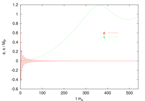
Figure 1: Evolution of the two scalar fields $\phi$ and $s$ for ${\hat{\mu}}^{2}=10^{-2}$.

We start our numerical calculations at ${\hat{\phi}}\simeq 1.4$, short after inflation, and with the scale factor $a$ normalized to one.

We show in figure 1 the evolution for the two scalar fields after inflation, in the case ${\hat{\mu}}^{2}=10^{-2}$. As we said, initially the model reproduces the scalar potential of chaotic inflation, and thus we have

$${\hat{\phi}}\simeq\sqrt{\frac{8}{3}}\,\frac{\cos\;{\hat{t}}}{{\hat{t}}}\,,\qquad{\hat{s}}\simeq 0\,.$$ (112)

The initial dynamics of the Polonyi field $s$ is determined by $\phi$. More precisely, we can write an effective potential $V(s)$ for it by substituting eq. (112) into $V(\phi,\,s)$ and then averaging over the inflaton oscillations. Expanding $V$ for both ${\hat{\phi}}$ and ${\hat{s}}$ smaller than one, we find that the potential is minimized by

$${\hat{s}}_{\min}\simeq\frac{\sqrt{2}\,{\hat{\mu}}^{2}[16\,{\hat{\beta}}\,{\hat{\mu}}^{2}-\langle{\hat{\phi}}^{4}\rangle]}{4\,\langle{\hat{\phi}}^{2}\rangle-16\,{\hat{\beta}^{2}}\,{\hat{\mu}}^{4}}\simeq\frac{3\,\sqrt{2}\,{\hat{\beta}}\left({\hat{\mu}}^{2}\,{\hat{t}}\right)^{2}}{1-3\,{\hat{\beta}}^{2}\left({\hat{\mu}}^{2}\,{\hat{t}}\right)}\,.$$ (113)

To be precise, the Polonyi field is always smaller than ${\hat{s}}_{\min}$, due to the fact that the expansion of the Universe slows its motion towards the minimum of $V(s)$. However, eq. (113) gives a good estimate for the order of magnitude of $s$ in this initial stage.

What is most important to emphasize, is that eqs. (112) and (113) explicitly show the presence of two very different (physical) time-scales in the model we are considering. The first of them is set by the inverse inflaton mass $m_{\phi}^{-1}$ which is the time-scale of the oscillations of the inflaton field. The second one is given by ${\hat{\mu}^{2}}\,m_{\phi}^{-1}$. Equation (113) shows that this is the relevant time-scale for the Polonyi field in the initial stage. However, this is true also for the complete evolution of $s$. To see this, let us consider the latest times shown in figure 1. In this stage the amplitude of the oscillations of $\phi$ are negligible. The evolution of $s$ is not any longer influenced by the inflaton field, but it starts oscillating about the minimum of its own potential given in eq. (108). The amplitude of these oscillations is also dumped by the expansion of the Universe, while their period is related to the inverse Polonyi mass, which is now (i.e. at $\phi=0$) given by [28]

$$m_{s}=\sqrt{2\,\sqrt{3}}\,m_{\tilde{G}}\simeq 2.4\,{\hat{\mu}}^{2}\,m_{\phi}\,.$$ (114)

The quantity ${\hat{\mu}}^{2}$ defines the ratio between the two scales. In figure 1 we have chosen, for illustrative purposes, ${\hat{\mu}}^{2}=10^{-2}$. However, this value is unphysical, since it would correspond to a too high supersymmetry breaking scale. Indeed, as eq. (109) shows, we must require ${\hat{\mu}}^{2}\sim 10^{-11}$, if supersymmetry is supposed to solve the hierarchy problem.

While the size of ${\hat{\mu}^{2}}$ controls the supersymmetry breaking in the vacuum of the theory, both scalar fields contribute to break supersymmetry during their evolution. In particular, both their kinetic and potential energies contribute to the breaking, as emphasized in ref. [18]. This can be seen by looking to the transformation law of the chiral fermions $\chi_{i}$ under an infinitesimal supersymmetry transformation with parameter $\varepsilon$. In our case they read

$$\delta\chi_{i}=-\frac{1}{2}\,P_{L}\,\left[m_{i}-\frac{1}{\sqrt{2}}\,\bar{\gamma}^{0}\,\frac{d\phi_{i}}{dt}\right]\varepsilon\,,$$ (115)

where $\phi_{1}=\phi,\ \phi_{2}=s$.

Following refs. [18, 19], we define the quantities

$$f_{\phi_{i}}^{2}\equiv m_{i}^{2}+\frac{1}{2}\left(\frac{d\phi_{i}}{dt}\right)^{2},$$ (116)

which give a “measure” of the size of the supersymmetry breaking provided by the $F$ term associated with the $i$-th scalar field. More precisely, we will be interested in the normalized quantities

$$r_{\phi}\equiv\frac{f_{1}^{2}}{f_{1}^{2}+f_{2}^{2}}\,,\qquad r_{s}\equiv\frac{f_{2}^{2}}{f_{1}^{2}+f_{2}^{2}}\,,$$ (117)

which indicate the relative contribution of the two scalar fields $\phi$ and $s$.

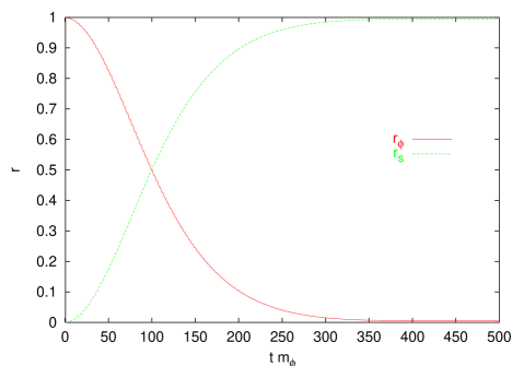
Figure 2: Relative contribution of the two scalar fields $\phi$ and $s$ to the supersymmetry breaking during their evolution. As in figure 1, ${\hat{\mu}}^{2}=10^{-2}$.

In figure 2 we have shown the evolution of $r_{\phi}$ and $r_{s}$ for the specific case ${\hat{\mu}}^{2}=10^{-2}$. As expected, in the initial stages only the inflaton contributes to the supersymmetry breaking, while only the Polonyi contributes at later times. The regime of equal contribution is around ${\hat{t}}={\hat{\mu}}^{-2}$, when $\phi$ and $s$ are of the same size (cf. figure 1). As it should be clear from the above discussion, $r_{\phi}$ and $r_{s}$ share the identical behavior for all the choices of ${\hat{\mu}}^{2}$, once ${\hat{t}}$ is given in units of ${\hat{\mu}}^{-2}$.

4.3 Effective fermionic lagrangian and hamiltonian in the case
of two chiral supermultiplets

The fermionic content of the model we are considering is of the gravitino $\psi_{\mu}$ and the two chiral fermions ${\tilde{\phi}}$ and ${\tilde{s}}$. In the unitary gauge, one combination of ${\tilde{\phi}}$ and ${\tilde{s}}$, the goldstino $\upsilon$, is set to zero, while the transverse component of the gravitino, $\psi_{i}^{T}$, is only gravitationally coupled to the other fields. The other two fermions $\theta$ (the longitudinal gravitino component) and $\Upsilon$ (the combination of chiral fermions orthogonal to $\upsilon$) are coupled together, as we described in section 4.1.

With some algebra, we can rewrite the initial lagrangian (89) in three terms

$$\mathcal{L}=\mathcal{L}_{\mathrm{background}}+\mathcal{L}_{\psi_{i}^{T}}+\mathcal{L}_{\theta\,\Upsilon}\,.$$ (118)

The first term governs the dynamics of the scalar fields and of the scale factor of the Universe. The second describes the (decoupled) transverse gravitino component, while the third one reads

$$\mathcal{L}_{\theta\,\Upsilon} = -\frac{\alpha}{4\,k^{2}}\,a^{3}\,\overline{\theta}\Bigg{[}\bar{\gamma}^{0}\,\partial_{0}\theta+i\,\bar{\gamma}^{i}\,k_{i}\hat{A}\,\theta+$$ (119)

$$\hphantom{-\frac{\alpha}{4\,k^{2}}\,a^{3}\,\overline{\theta}\Bigg{[}}\!-\left(\frac{3}{2}\,\dot{a}\,\bar{\gamma}^{0}+\frac{3}{2\,M_{\mathrm{P}}^{2}}\,a\,m\right)\hat{A}\,\theta-\frac{a\,m}{2\,M_{\mathrm{P}}^{2}}\,\theta-\frac{4\,k^{2}}{\alpha\,a}\,\bar{\gamma}^{0}\,\Upsilon\Bigg{]}+$$

$$-\,\frac{4\,a}{\alpha\,\Delta^{2}}\,\overline{\Upsilon}\Bigg{[}\bar{\gamma}^{0}\,\partial_{0}\Upsilon-i\,\bar{\gamma}^{i}\,k_{i}\hat{A}\,\Upsilon-\frac{3}{2}\,\dot{a}\,\bar{\gamma}^{0}\,\hat{A}\,\Upsilon+\frac{3}{2\,M_{\mathrm{P}}^{2}}\,\hat{A}\,a\,m\,\Upsilon+$$

$$\hphantom{-\,\frac{4\,a}{\alpha\,\Delta^{2}}\,\overline{\Upsilon}\Bigg{[}}\!+\,2\,\dot{a}\,\bar{\gamma}^{0}\,\Upsilon-\frac{a\,m}{2\,M_{\mathrm{P}}^{2}}\,\Upsilon+\frac{1}{4}\,a\,\alpha\,\Delta^{2}\,\bar{\gamma}^{0}\,\theta\Bigg{]}\,.$$

We have expanded the fermions into plane waves $X_{i}(\eta,\,\mathbf{k})=\mathrm{e}^{i\,{k_{i}x^{i}}}\,X_{i}(\eta)$, where $k_{i}$ is the comoving momentum (i.e. $\partial_{0}\,k_{i}=0)$, and we have introduced

$$\Delta \equiv \frac{2}{\alpha}\left[\dot{\phi}_{i}\,\dot{\phi_{j}}\,m_{k}m_{l}\left({g^{-1}}_{kl}\,g_{ij}-\delta_{ik}\,\delta_{lj}\right)\right]^{1/2}$$ (120)

$$= \frac{2}{\alpha}\left(m_{1}\dot{\phi}_{2}-m_{2}\dot{\phi}_{1}\right),$$

where the second equality holds in the case of a minimal Kähler potential, $g_{i}^{j}=\delta_{i}^{j}$. The quantity $\Delta$ has no counterpart in the one chiral superfield case, and indeed it is negligible unless both the scalar fields give a sizeable contribution to the breaking of supersymmetry.

One can explicitly verify that the lagrangian (119) reproduces the equation of motion (103) for the longitudinal gravitino component, as well as the one for $\Upsilon$ that one obtains from the initial lagrangian (89). However, we notice that the two fields $\theta$ and $\Upsilon$ are not canonically normalized. Canonical normalization has to be imposed, if we want our fields to give invariant quantities (as for example the occupation number) in comoving units in the adiabatic regime. Among the possible redefinitions, we choose

$$\theta = \frac{2\,i\,\bar{\gamma}^{i}\,k_{i}}{\left(\alpha\,a^{3}\right)^{1/2}}\,{\tilde{\theta}}\,,$$

$$\Upsilon = \frac{\Delta}{2}\left(\frac{\alpha}{a}\right)^{1/2}{\tilde{\Upsilon}}\,,$$ (121)

since the equations of motion look quite symmetric in terms of the new fields. In matrix form, they are exactly of the form (63), i.e.

$$\left(\bar{\gamma}^{0}\,\partial_{0}+i\,\bar{\gamma}^{i}\,k_{i}N+M\right)X=0\,,$$ (122)

where $X$ is the vector $({\tilde{\theta}},{\tilde{\Upsilon}})^{T}$. In our specific case, the “mass” matrix $M$ is given by

$$M = \mathop{\rm diag}\nolimits\left(\frac{m\,a}{2\,M_{\mathrm{P}}^{2}}+\,\frac{3}{2}\,\left(\frac{m\,a}{M_{\mathrm{P}}^{2}}\,{\tilde{\alpha}}_{1}+\dot{a}\,{\tilde{\alpha}}_{2}\right)\right.-$$ (123)

$$\hphantom{\mathop{\rm diag}\nolimits\Bigg{(}}\!\left.-\,\frac{m\,a}{2\,M_{\mathrm{P}}^{2}}+\,\frac{3}{2}\left(\frac{m\,a}{M_{\mathrm{P}}^{2}}\,{\tilde{\alpha}}_{1}+\dot{a}\,{\tilde{\alpha}}_{2}\right)+a\left(m_{11}+m_{22}\right)\right),$$

and the $N$ matrix by

$$N\equiv N_{1}+\bar{\gamma}^{0}\,N_{2}=\pmatrix{-{\tilde{\alpha}}_{1}&0\cr 0&-{\tilde{\alpha}}_{1}}+\bar{\gamma}^{0}\pmatrix{-{\tilde{\alpha}}_{2}&-\Delta\cr-\Delta&{\tilde{\alpha}}_{2}}.$$ (124)

In the above equations, we have defined ${\tilde{\alpha}}_{i}\equiv\alpha_{i}/\alpha$. The relation ${\tilde{\alpha}}_{1}^{2}+{\tilde{\alpha}}_{2}^{2}\equiv 1$ which holds in the one chiral field case [14, 15] is now replaced by

$${\tilde{\alpha}}_{1}^{2}+{\tilde{\alpha}}_{2}^{2}+\Delta^{2}\equiv 1\,.$$ (125)

We thus see that the matrices $N_{1}$ and $N_{2}$ satisfy both conditions (65).

The equations of motion (122) have a clear behavior in the low energy limit, when the two scalars of the theory settle to their minima. In this final stage one has ${\tilde{\alpha}}_{1}=-1,{\tilde{\alpha}}_{2}=\Delta=0$, as it can be easily checked from the definitions listed above. As a consequence, eqs. (122) decouple, and each of them acquires the standard form for spin $1/2$ fermions

$$\left(\bar{\gamma}^{0}\,\partial_{0}+i\,\bar{\gamma}^{i}\,k_{i}+a\,m_{\tilde{\theta}}\right){\tilde{\theta}} = 0\,,$$

$$\left(\bar{\gamma}^{0}\,\partial_{0}+i\,\bar{\gamma}^{i}\,k_{i}+a\,m_{\tilde{\Upsilon}}\right){\tilde{\Upsilon}} = 0\,,$$ (126)

where the two masses are constant. In particular, notice that $m_{\tilde{\theta}}=m/M_{\mathrm{P}}^{2}$, which is exactly the expression that one encounters in supergravity for the gravitino mass.

We thus see that the system has all the properties assumed in section (3.2), so that we can apply the procedure derived there to quantize it and to define the occupation numbers of the fermionic eigenstates. Among the possible choices for the transformation matrix $\Phi$ which enters into eq. (66), we take

$$\Phi=\frac{1}{2}\left(\mbox{arccos}\;\;{\tilde{\alpha}}_{1}\right)\pmatrix{{\tilde{\alpha}}_{2}/\omega&\Delta/\omega\cr\Delta/\omega&-{\tilde{\alpha}}_{2}/\omega},$$ (127)

with

$$\omega\equiv\sqrt{1-{\tilde{\alpha}}_{1}^{2}}=\sqrt{{\tilde{\alpha}}_{2}^{2}+\Delta^{2}}\,.$$ (128)

Following eq. (74), the hamiltonian of the system is instead given by

$$H={\bar{X}}\left[i\,\bar{\gamma}^{i}\,k_{i}N+{\tilde{M}}_{1}+\bar{\gamma}^{0}\,{\tilde{M}}_{2}\right]X\,,$$ (130)

with

$${\tilde{M}}_{1} \equiv M+\frac{\omega^{2}}{2}\left(Q\,M\,Q-M\right)+\frac{\partial_{0}\,{\tilde{\alpha}}_{1}}{2\,\omega}\,Q-\frac{\omega}{2}\,{\tilde{\alpha}}_{1}\,\partial_{0}\,Q\,,$$

$${\tilde{M}}_{2} \equiv \frac{\omega\,{\tilde{\alpha}}_{1}}{2}\left[M,\,Q\right]+\frac{\omega^{2}}{4}\left[Q,\,\partial_{0}\,Q\right].$$ (131)

We have denoted

$$Q=\pmatrix{{\tilde{\alpha}}_{2}/\omega&\Delta/\omega\cr\Delta/\omega&-{\tilde{\alpha}}_{2}/\omega}.$$ (132)

As we have already remarked, at late times ${\tilde{\alpha}}_{1}=-1$, while ${\tilde{\alpha}}_{2}=\Delta=0$. In this regime the above hamiltonian becomes the standard one of two decoupled spin $1/2$ fermions

$$H={\bar{X}}\left[i\,\bar{\gamma}^{i}\,k_{i}+M\right]X\,,$$ (133)

with the standard gravitino mass for the field ${\tilde{\theta}}$ (cf. eq. (126)).

We conclude this subsection discussing the explicit diagonalization of the hamiltonian, i.e. of the matrices $\overline{H}$ and $\overline{H}_{0}$ entering in eqs. (82) and (83). One can now explicitly verify that the eigenvalues of the $\overline{H}_{0}$ matrix occur in pairs, that is they are of the form $\pm\omega_{1},\pm\omega_{2}$. One can also verify that if $(v_{1},\,v_{2},\,v_{3},\,v_{4})$ is an eigenvector of $\overline{H}_{0}$ belonging to the eigenvalue $\omega$, then $(-v_{3}^{*},-v_{4}^{*},\,v_{1}^{*},\,v_{2}^{*})$ is also an eigenvector of $\overline{H}_{0}$ belonging to the eigenvalue $-\omega$. We then find

$$R^{\dagger}\>\overline{H}_{0}\>R=H_{d}\,,\qquad R=\pmatrix{R_{1}&-R_{2}^{*}\cr R_{2}&R_{1}^{*}},$$ (134)

where $H_{d}=\mathop{\rm diag}\nolimits(\omega_{1},\,\omega_{2},-\omega_{1},-\omega_{2})$ is the matrix that we formally introduced in eq. (81).

The $2\times 2$ matrices defined by eq. (86) are thus given by

$$I = \frac{1}{\sqrt{2}}\left[R_{1}^{\dagger}\,U_{+}+R_{2}^{T}\,U_{-}\right],$$

$$J = \frac{i}{\sqrt{2}}\left[-R_{1}^{\dagger}\,U_{-}^{*}+R_{2}^{T}\,U_{+}^{*}\right].$$ (135)

We remind that the matrices $R_{1}$ and $R_{2}$ are obtained through the diagonalization of $\overline{H}_{0}$ see eq. (134). The matrices $U_{+}$ and $U_{-}$ are instead determined by their evolution equation (77). The only point left is to give more explicitly their values at the initial time $\overline{\eta}$. This can be done by setting $J=0$ in eq. (135), which, as we remarked, corresponds to requiring no fermions in the initial state (see eq. (88)). Moreover, conditions (78) have to be imposed. From these requirements, we see that $U_{+}(\overline{\eta})$ has to fulfill

$$U_{+}^{\dagger}\left(\overline{\eta}\right)\left[\mathbbm{1}+R_{2}\left(\overline{\eta}\right)R_{1}^{*-1}\left(\overline{\eta}\right)R_{1}^{T-1}\left(\overline{\eta}\right)R_{2}^{\dagger}\left(\overline{\eta}\right)\right]U_{+}\left(\overline{\eta}\right)=2\,\mathbbm{1}\,.$$ (136)

In this last expression, the matrix in square brackets is hermitean and can be diagonalized with a unitary transformation. More precisely, we can set it to be equal to $V^{\dagger}\,\Lambda\,V$ with $\Lambda$ diagonal and real, and $V$ unitary. The initial condition for $U_{+}$ can thus be written

$$U_{+}\left(\overline{\eta}\right)=V^{\dagger}\,\sqrt{2\,\Lambda^{-1}}\,.$$ (137)

Finally, $U_{-}(\overline{\eta})$ is obtained by setting $J(\overline{\eta})=0$ in eq. (135).

4.4 Analytical results with unbroken supersymmetry in the vacuum

The case ${\hat{\mu}}^{2}=0$ is particularly interesting since some results can be worked out analytically, and since it provides some hints between the final gravitino abundance and the size of supersymmetry breaking. For ${\hat{\mu}}^{2}=0$ supersymmetry is unbroken in the minimum of the theory, at $\phi=s=0$. Because of this, in the vacuum of the theory the gravitino has only the transverse component.

The computation of the formulae of section 4.3 is in this case particularly simplified. The quantity $\Delta$ vanishes identically, so that the two fields $\Upsilon$ (which is always the Polonyi fermion) and $\theta$ (which is always the inflatino) are decoupled. Going back to the formalism of section (3.2), we find that we have to perform only the first redefinition of the fermions, $X\equiv\exp(-\bar{\gamma}^{0}\,\Phi)\,{\hat{X}}$, where now $\Phi=\mathop{\rm diag}\nolimits(\varphi,-\varphi)$, with

$$\cos\left(2\,\varphi\right)={\tilde{\alpha}}_{1}\,,\qquad\sin\left(2\,\varphi\right)={\tilde{\alpha}}_{2}\,.$$ (138)

The two redefined fields have the “standard” equations of motion and hamiltonian

$$\left(\bar{\gamma}^{0}\,\partial_{0}+i\,\bar{\gamma}^{i}\,k_{i}+m_{\hat{\theta}}\right){\hat{\theta}} = 0\,,$$

$$\left(\bar{\gamma}^{0}\,\partial_{0}+i\,\bar{\gamma}^{i}\,k_{i}+m_{\hat{\Upsilon}}\right){\hat{\Upsilon}} = 0\,,$$

$$H = \int d^{3}\mathbf{k}\left[{\bar{\hat{\theta}}}\left(i\,\bar{\gamma}^{i}\,k_{i}+m_{\hat{\theta}}\right){\hat{\theta}}+{\bar{\hat{\Upsilon}}}\left(i\,\bar{\gamma}^{i}\,k_{i}+m_{\hat{\Upsilon}}\right){\hat{\Upsilon}}\right],$$

$$m_{\hat{\theta}} = m_{\theta}+\partial_{0}\varphi\,,\qquad m_{\hat{\Upsilon}}=m_{\Upsilon}-\partial_{0}\varphi\,,$$ (139)

with $m_{\theta}$ and $m_{\Upsilon}$ given in eq. (123).

In practice, “removing” the time dependent matrix which multiplies the momentum in the original equations for $\theta$ and $\Upsilon$ gives an additional contribution to the mass of the fields ${\hat{\theta}}$ and ${\hat{\Upsilon}}$, as noticed in [14, 15]. When $\Delta=0$, an explicit computation of $\partial_{0}\phi$ with the present formalism is provided in [19]

$$\partial_{0}\varphi=-a\,\frac{\dot{{\tilde{\alpha}}_{2}}}{2\,{\tilde{\alpha}}_{1}}=a\,\left(m_{11}+m\right)+3\,a\,\left(H\,\frac{\dot{\phi}}{\sqrt{2}}-m_{1}\,m\right)\frac{m_{1}}{\frac{1}{2}\,\dot{\phi}^{2}+m_{1}^{2}}\,,$$ (140)

where the various quantities have been introduced in section 4.1. Using the equation of motion for the inflaton field $\phi$, one can show that it is precisely $\partial_{0}\varphi\equiv m_{\Upsilon}$, so that the field ${\hat{\Upsilon}}$ is effectively massless. The mass for ${\hat{\theta}}$ is instead of the order the inflaton mass. More precisely, it has a variation of the order $m_{\phi}$ within the first oscillation of the inflaton (i.e. in the time $m_{\phi}^{-1}$) and then it stabilizes at $m_{\phi}$ [14, 15]. Since the fields are decoupled, the formulae for the occupation numbers (47) are quite simple. They show that the Polonyi fermion is not produced, while the production of the inflatino field has a cut-off at $k\sim m_{\phi}$, and decreases as $k^{-4}$ at big momenta.

The main point of this subsection is that the Polonyi fermion is not produced at preheating for ${\hat{\mu}}^{2}$ strictly zero. When ${\hat{\mu}}^{2}\neq 0$ the Polonyi fermion provides the longitudinal component for the gravitino, so its abundance turns out crucial to understand whether gravitinos are or are not overproduced. If one believes that the limit ${\hat{\mu}}^{2}\rightarrow 0$ is continuous, the present analysis suggests indeed that the production of gravitinos should become smaller as ${\hat{\mu}}^{2}$ decreases. Although we do not have a rigorous proof of this continuous behavior, the numerical results that we show in the next subsection strongly support this assumption.

4.5 Numerical results with broken supersymmetry in the vacuum

We now analyze the situation ${\hat{\mu}}^{2}\neq 0$. As we have said, in this case the quantity $\Delta$ is generally also non vanishing in the most interesting part of the evolution. As a consequence, the dynamics of the fermionic fields ${\tilde{\theta}}$ and ${\tilde{\Upsilon}}$ is coupled, i.e. we have mixed terms in their equations of motion (122) and in their hamiltonian (130). For the following discussion it is useful to explicitly write ${\tilde{\Upsilon}}$ in terms of the chiral fields $\chi_{1}$ and $\chi_{2}$. Combining the definitions (104), (120), and (127) we have, for minimal Kähler potential and real scalar fields,

$${\tilde{\Upsilon}}=\frac{a^{3/2}[m_{1}^{2}+m_{2}^{2}+\frac{1}{2}\,\dot{\phi}_{1}^{2}+\frac{1}{2}\,\dot{\phi}_{2}^{2}]^{1/2}}{m_{1}\,\dot{\phi}_{2}^{2}-m_{2}\,\dot{\phi}_{1}^{2}}\left(\dot{\phi}_{1}\,\chi_{1}+\dot{\phi}_{2}\,\chi_{2}\right),$$ (141)

where we remind that the two scalars $\phi_{1}$ and $\phi_{2}$ are the inflaton and the Polonyi field, while $\chi_{1}$ and $\chi_{2}$ the corresponding fermions. Moreover, the definition (98) of the goldstino now reads

$$\upsilon_{L}=\left(m_{i}-\frac{1}{\sqrt{2}}\,\bar{\gamma}^{0}\,a\,\dot{\phi}_{i}\right)\chi_{i}\,.$$ (142)

Let us first consider the initial and final stages of the evolution, where only one of the two scalar fields significantly contribute to the supersymmetry breaking and the quantity $\Delta$ is practically vanishing. During inflation, one has $m_{2},\,\dot{\phi}_{1},\,\dot{\phi}_{2}\simeq 0$, and the supersymmetry breaking is provided almost completely by $m_{1}$. Moreover, the goldstino is practically the field $\chi_{1}$. We remind that we are working in the unitary gauge, so that $\chi_{1}\simeq\upsilon=0$. Equation (141) thus rewrites

$${\tilde{\Upsilon}}\simeq\frac{a^{3/2}\,|m_{1}|}{m_{1}\,\dot{\phi}_{2}}\,\chi_{1}\,\dot{\phi}_{2}=a^{3/2}\,\chi_{1}\,,\qquad{\hat{t}}\ll{\hat{\mu}}^{-2}\,.$$ (143)

Notice the factor $a^{3/2}$ appearing in the last expression, which is a consequence of the fact that the field ${\tilde{\Upsilon}}$ is canonically normalized in comoving units (cf. the discussion after the lagrangian (119)). In the late stages of the evolution, supersymmetry is instead broken by the Polonyi field, and the only non-vanishing contribution is provided by $m_{2}$. With the same arguments used to get eq. (143), one can show that

$$\upsilon\propto\chi_{2}=0\,,\qquad{\tilde{\Upsilon}}=-a^{3/2}\,\chi_{1}\,,\qquad{\hat{t}}\gg{\hat{\mu}}^{-2}\,.$$ (144)

In order to compute the evolution of the occupation number of the fermions we adopt the procedure described in section 3.2: during the evolution of the system, the states are mixed in such a way that the hamiltonian is kept in a diagonal form. The two eigenstates obtained through this diagonalization coincide with the fields $\theta$ and $\Upsilon$ only for $\Delta=0$. In particular, this is true at very early and late times. The safest way to make the proper identifications in these regimes is to consider the evolution of the mass eigenvalues, which always behave like in the example shown in figure 3. The two masses present (for ${\hat{\mu}}^{-2}\ll 1$) a strong hierarchy. We denote with $\psi_{1}$ the eigenstate with bigger mass, and with $\psi_{2}$ the other one. The mass of $\psi_{1}$ converges to the inflatino mass ($\simeq 1.31~{}m_{\phi}$) at late times, and it is always of the order $m_{\phi}$. On the contrary, the mass of $\psi_{2}$ converges to the gravitino mass ($\simeq 1.31~{}\hat{\mu}^{2}\,m_{\phi}$) in the vacuum. As it will be clear below, we can “qualitatively” identify $\psi_{1}$ with the inflatino and $\psi_{2}$ with the Polonyi fermion for the whole evolution. Although rigorous only at late times, this identification can be useful for a qualitative understanding of the system.

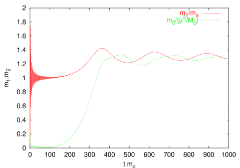
Figure 3: Evolution of the masses of the two fermionic eigenstates. As in figure 1, ${\hat{\mu}}^{2}=10^{-2}$. Notice the different normalizations for the two masses.

What is most important to us is the relation between the eigenstates $(\psi_{1},\,\psi_{2})$ and the gravitino $\theta$ and the matter field $\Upsilon$. As we have said, the last fields coincide with the physical eigenstates only at the very beginning and at the end of the evolution. More precisely, from the behavior of the two masses we have

$$\theta\equiv\psi_{2}\qquad\mbox{and}\qquad\Upsilon\equiv\psi_{1}$$ (145)

at late times. On the contrary, it must be

$$\theta\equiv\psi_{1}\qquad\mbox{and}\qquad\Upsilon\equiv\psi_{2}$$ (146)

at early times, since the longitudinal gravitino component $\theta$ is provided by the goldstino and supersymmetry is initially broken only by the inflaton field.

At intermediate times, the hamiltonian cannot be diagonalized with a simple rotation in “flavor” space, and $\theta$ cannot be just a simple (i.e. with only numbers as coefficients) linear combination of $\psi_{1}$ and $\psi_{2}$. However, we can gain an intuitive description of the system through the identifications

$$\theta \sim \sqrt{r_{\phi}}\,\psi_{1}+\sqrt{r_{s}}\,\psi_{2}\,,$$

$$\Upsilon \sim -\sqrt{r_{s}}\,\psi_{1}+\sqrt{r_{\phi}}\,\psi_{2}\,.$$ (147)

The coefficients $r_{\phi}$ and $r_{s}$ give a “measure” of the relative contribution to supersymmetry breaking provided by the two scalar fields (see eq. (117)). These relations can thus be justified as a “generalization” of the equivalence theorem, in a way also suggested in [18, 19]. We remark that they are rigorous at early and late times (when they coincide with the identifications (145) and (146)). At intermediate times they interpolate between these two regimes and can be thus used as a qualitative description of the system.

From eqs. (147) we deduce the following estimates for the occupation numbers

$$N_{\theta} = r_{\phi}\,N_{1}+r_{s}\,N_{2}\,,$$

$$N_{\Upsilon} = r_{s}\,N_{1}+r_{\phi}\,N_{2}\,.$$ (148)

The evolution of these quantities is shown in figure 4 for modes of comoving momentum $k=m_{\phi}$ and for ${\hat{\mu}}^{2}=10^{-2}$. Notice that (by construction) $N_{\theta}\equiv N_{1}$ at early times, while $N_{\theta}\equiv N_{2}$ at late ones. In these regimes these identifications are rigorous.

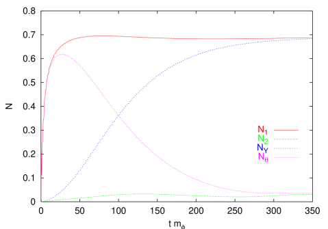
Figure 4: Evolution of $N_{\theta}$ and $N_{\Upsilon}$ for ${\hat{\mu}}^{2}=10^{-2}$ and $k=m_{\phi}$. See the text for details.

In figures 5 and 6 we plot instead the spectra of the states $\psi_{1}$ and $\psi_{2}$ in the case ${\hat{\mu}}^{2}=10^{-2}$ and at the times $t=10\,m_{\phi}^{-1}$ (that is, after a couple of oscillations of the inflaton), $t=\hat{\mu}^{-2}\,m_{\phi}^{-1}$, and $t=10\,\hat{\mu}^{-2}\,m_{\phi}^{-1}$.

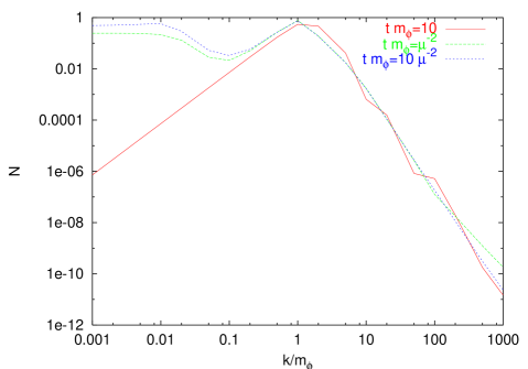
Figure 5: Spectrum of the state $\psi_{1}$ at different times for $\hat{\mu}^{2}=10^{-6}$.

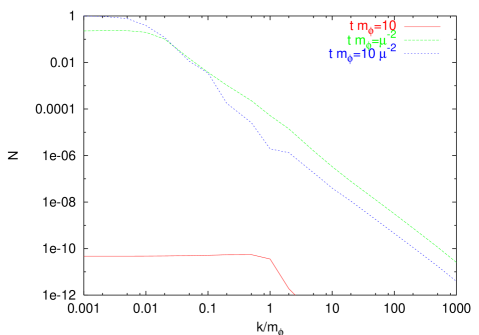
Figure 6: Spectrum of the state $\psi_{2}$ at different times for $\hat{\mu}^{2}=10^{-6}$.

It is apparent that most quanta of the state $\psi_{1}$ are produced at the very first oscillations of the inflaton field, while quanta of $\psi_{2}$ are mainly produced at the times when the Polonyi scalar starts oscillating. This supports the qualitative identification of $\psi_{1}$ with the inflatino and of $\psi_{2}$ with the Polonyi fermion. It is worth noticing that, for comoving momenta smaller than $m_{\phi}$, the increase of $N_{2}$ is not related to a “conversion” of quanta of $\psi_{1}$ to $\psi_{2}$. Indeed, the increase in $N_{2}(k)$ is not accompanied by a decrease in $N_{1}(k)$ for $k\lesssim m_{\phi}$.

We can now show our most important result, that is the spectra of $\Upsilon$ and $\theta$ at the end of the process. We present them in figures 7 and 8, respectively. They are computed at the time $t=10\,{\hat{\mu}}^{-2}m_{\phi}^{-1}$. The time required for the numerical computation increases linearly with ${\hat{\mu}}^{2}$, and the realistic case ${\hat{\mu}}^{2}=10^{-11}$ is far from our available resources. We thus kept $\hat{\mu}^{2}$ as a free parameter and we performed the explicit numerical computation only up to $\hat{\mu}^{2}=10^{-6}$. In particular, in figures 7 and 8 the spectra of the fermions produced at preheating are shown for $\hat{\mu}^{2}=10^{-2},\,10^{-3},\,10^{-4},\,10^{-5},\,10^{-6}$. The case ${\hat{\mu}}^{2}=10^{-11}$ can be clearly extrapolated from the ones shown in these figures.

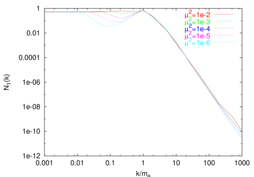
Figure 7: Spectrum of inflatinos at late times.

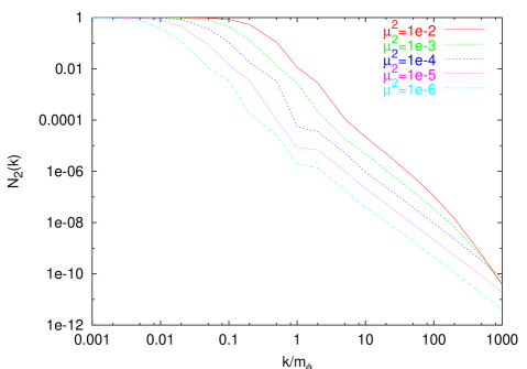
Figure 8: Spectrum of gravitinos at late times.

In figure 7, the spectra for the state $\psi_{1}$ are shown. This state corresponds to the matter fermion $\Upsilon$ in the true vacuum. It is apparent that the main features of the spectrum are independent of the value of $\hat{\mu}^{2}$. The reason for this is that $\psi_{1}$ is associated to the inflatino, that is produced by the coherent oscillations of the inflaton. As we discussed above, the dynamics responsible for the production of this state is independent on the value of $\hat{\mu}^{2}$. Therefore the only relevant scale for $N_{1}$ is $m_{\phi}$, and indeed the spectrum of $\psi_{1}$ exhibits a cut-off at comoving momentum $k\sim m_{\phi}$.

The spectra shown in figure 8 are related to the abundance of gravitinos after the fields have stabilized in their minima. We see that in this case the occupation number decreases as $\hat{\mu}^{2}$ becomes smaller. Indeed, the occupation number $N_{2}(k)$ is of order unity for comoving momenta $k$ smaller than some cut-off $k_{*}$. From figure 8 we can deduce the dependence $k_{*}\propto(\hat{\mu}^{2})^{1/3}$ of this cut-off on the parameter ${\hat{\mu}}^{2}$. This behavior suggests that gravitinos are not produced in the limit ${\hat{\mu}}^{2}\rightarrow 0$, confirming what we have argued in the section 4.4.

We can conclude that in the model we are considering both inflatinos and gravitinos are produced nonthermally. However, the mechanism responsible for the production of gravitinos is much less efficient that the one acting on inflatinos. Indeed, the latter is related to the dynamics of the inflaton, while the former is related to the dynamics of the Polonyi field. As a consequence, and as it is clearly confirmed by the comparison of figures 7 and 8, the number of non-thermal gravitinos is much smaller than the number of inflatinos.

5 Conclusions

Particles with gravitational decay constitute one of the most serious danger for cosmology, since they can spoil the successful predictions of primordial nucleosynthesis. This is particularly true for gravitinos in models where supersymmetry is gravitationally broken. To avoid this danger, strong upper limits must be imposed on their number. While gravitino thermal production has been very well studied and understood over the last twenty years, only very recently non-perturbative creation after inflation has been considered. Non-perturbative production appears more involved than the thermal one, and indeed explicit calculations were so far performed only in the one superfield case with supersymmetry unbroken in the vacuum. The results of these calculations showed that the coherent oscillations of the inflaton field easily cause an overproduction of the longitudinal gravitino component. However, this component is absent in the vacuum of the theory if supersymmetry is unbroken. One is thus led to wonder if these quanta are really dangerous gravitinos or should be better understood as harmless inflatinos (in case of only one chiral multiplet, the scalar is necessary the inflaton). In order to discriminate between inflatino and gravitino production it is necessary to consider more realistic schemes. The simplest natural possibility is to consider two separate sectors, one of which drives inflation, while the second is responsible for supersymmetry breaking today. In the present analysis we have studied the situation in which the two sectors communicate only gravitationally, in the hope that suppressing their interaction may lead to a small gravitino production.

The presence of more than one chiral superfield increases the difficulty of the problem. One has to deal with a (quite involved) coupled system, constituted by the gravitino longitudinal component and some combinations of the matter fields, in the external background made by the scalar fields of the theory. The most difficult part of this analysis is to provide a formalism in which the coupled system is quantized, with a clear definition of the occupation numbers for the physical eigenstates. This is a very interesting problem by itself, which can have several other applications besides the gravitino production. We faced this problem in the first part of the work. We showed that the standard procedure for quantizing and providing the occupation number for one field can be generalized to systems of multi coupled fields, both in the bosonic and in the fermionic case. Although far from trivial, this generalization can be presented in a remarkably simple form. The application of this formalism to the gravitino production is performed in the last section of the paper. We have shown that, in the specific model considered here, the number of produced gravitinos is very sensitive to the size of the final supersymmetry breaking, and that it actually vanishes in the limit in which supersymmetry is preserved. Due to the small scale of the expected supersymmetry breakdown, we conclude that gravitino non-thermal production is very suppressed in this model.

Note added.

Contemporarily to the present manuscript, the work [29] appeared on the database. This work does not consider gravitinos, but studies the non-thermal production of moduli fields coupled to the inflaton sector. Moduli fields can also be very dangerous for cosmology because, analogously to gravitinos, they are expected to decay gravitationally. The work [29] shows that moduli production can be significant if — after inflation — they are strongly coupled to the inflaton. These considerations seem to agree with our suggestion [23] that strong couplings between potentially dangerous relics (in our case gravitinos) and the inflaton sector should be avoided in any viable cosmological model.