Aspects of Gauge Theory on Commutative
and Non-commutative Tori

Zachary Guralnik and Jan Troost

Center for Theoretical Physics
Massachusetts Institute of Technology
Cambridge MA, 02139
Email: zack@mitlns.mit.edu,troost@mit.edu

Abstract

We study aspects of gauge theory on tori which are a consequences of Morita equivalence. In particular we study the behavior of gauge theory on non-commutative tori for arbitrarily close rational values of $\Theta$. For such values of $\Theta$, there are Morita equivalent descriptions in terms of Yang-Mills theories on commutative tori with very different magnetic fluxes and rank. In order for the correlators of open Wilson lines to depend smoothly on $\Theta$, the correlators of closed Wilson lines in the commutative Yang-Mills theory must satisfy strong constraints. If exactly satisfied, these constraints give relations between small and large $N$ gauge theories. We verify that these constraints are obeyed at leading order in the $1/N$ expansion of pure 2-d QCD and of strongly coupled ${\cal N}=4$ super Yang-Mills theory.

1 Introduction

The subject of gauge theory on non-commutative spaces has received much attention recently for a variety of reasons. In string theory, interest in the subject was kindled by [1] where it arose in the context of toroidal compactification of M(atrix) theory corresponding to eleven dimensional supergravity backgrounds with a constant three-form field. In [2], it was shown that non-commutative gauge theories arise naturally in IIA/B string theory as a certain decoupling limit of D-branes in NS-NS two-form backgrounds. In this paper we shall be interested in the behavior of gauge theories on non-commutative tori. In particular we shall study the question of how smoothly the non-commutative theory depends on the non-commutativity parameter $\Theta$ on a spacelike $T^{2}$. Our motivation for addressing this question is that continuity in $\Theta$ has strong consequences for the behavior of commutative gauge theories, due to the Morita equivalence [3] between commutative and non-commutative spaces for rational $\Theta$.

The question of smoothness in $\Theta$ was addressed in part in [4], following the work of [5]. These authors noticed different high energy behavior for rational and irrational $\Theta$. As one increases the energy, there is a sequence of T-dual (or Morita equivalent) descriptions such that the theory has a quasi-local description. In the rational case, this sequence terminates above some finite energy, whereas in the irrational case the sequence never terminates. Since any irrational number is arbitrarily close to a rational one, the theory does not depend smoothly on $\Theta$ from this point of view. On the other hand, if one varies $\Theta$ at a fixed energy, then the behavior is essentially smooth. Only at certain isolated values of $\Theta$ does the quasi-local T-dual description change. Note that these are not really phase transition points, and so do not represent any non-smooth behavior of the physics.

In fact, whether or not things depend smoothly on $\Theta$ seems to depend on the question one asks. For instance, the moduli space of flat connections is independent of $\Theta$ [6] (and therefore depends smoothly on $\Theta$). However the periodicity of non-commutative gauge fields for instance does not depend smoothly on $\Theta$. A natural question is whether correlation functions open Wilson lines with fixed transverse momenta depend continuously on $\Theta$.

One way to address the question of continuity is to consider arbitarily close rational values of $\Theta$. For rational $\Theta$ there is a Morita equivalent description in terms of a $U(N)$ Yang-Mills theory with magnetic flux $m$ on a commutative torus [1, 2, 9, 10]. The rank $N$ and flux $m$ of the commutative description differ drastically for arbitarily close rational values of $\Theta$. If for instance one considers the $U(1)$ gauge theory on a non-commutative $T^{2}$ with $\Theta=-c/N$ for integer $c$ and $N$, then the dual commutative theory has rank $N$ and flux $m$ which are solutions of $aN-cm=1$, where $a$ is integer. Thus the commutative dual for $\Theta=-1/2$ is a $U(2)$ gauge theory, whereas the commutative dual for $\Theta=-1000/2001$ is an $U(2001)$ gauge theory. It follows that for open Wilson line correlators to depend smoothly on $\Theta$ – up to some possible isolated phase transition points in $\Theta$ –, there must be relations between commutative gauge theories of very different rank. For this reason, smooth dependence of correlators on $\Theta$ is a very non-trivial phenomenon. Yet continuity seems likely, at least in cases in which the non-commutative Yang-Mills theory is obtained from string theory, where the NS-NS two form is a continuous background. Comparing the small and large $N$ gauge theories is beyond the scope of this paper. However we will be able to check some of the properties implied by smooth $\Theta$ dependence in the large $N$ expansion of commutative gauge theories.

The T-duality which relates the non-commutative theory to the commutative one maps open Wilson lines of the non-commutative theory to closed Wilson lines wrapping the torus of the commutative theory [11, 12]. Thus the condition that the open Wilson line correlators depend smoothly on $\Theta$ can be translated into a condition satisfied by correlators of wrapped Wilson loops in the commutative theory. The latter can only depend on certain combinations of $m$, $N$, the radius $R$, the coupling $g^{2}$, and the winding number and transverse momenta of the wrapped Wilson loops. (In asymptotically free theories, $g^{2}$ is replaced by the QCD scale.) We find that the Wilson loop correlators have the required dependence on these variables at leading order in the $1/N$ expansion of the strongly coupled four dimensional ${\cal N}=4$ super Yang-Mills theory. In pure two-dimensional Yang-Mills, we shall also find the correct behavior at leading order in the $1/N$ expansion. In both cases, the smooth behavior depends crucially on the fact that the magnetic flux behaves as a $B$ field modulus in a string description of the Yang-Mills theory.

The organization of this paper is as follows. In section 2 we review the definition of gauge theory on a non-commutative torus. In section 3, we give a simple construction of the Morita equivalence between a $U(1)$ gauge theory compactified on a non-commutative $T^{2}$ with rational $\Theta$ and a $U(N)$ Yang-Mills theory on a commutative torus with magnetic flux. Morita equivalence was explicitly shown in generality in [9]. The non-smooth dependence of the gauge field periodicity on $\Theta$ follows simply from this map. In section 4 we construct the map between open Wilson lines [11, 12] (including possible local operator insertions) in the non-commutative theory and wrapped Wilson lines in the commutative dual. In section 5 we discuss the correlation functions of wrapped Wilson loops in large N strongly coupled large ${\cal N}=4$ super Yang-Mills theory using the AdS-CFT correspondence, and show that at least to leading order in $1/N$ these have the behavior predicted by continuity in $\Theta$. We also discuss confining Yang-Mills theory in the $1/N$ expansion, and find behavior consistent with continuity in $\Theta$. In section 6 we discuss other possible tests of smooth behavior, and give our conclusions.

2 Review of Non-commutative Gauge Theories

Gauge theory on a non-commutative space can be constructed essentially by replacing regular products of functions with Moyal star products. The star product is defined as follows:

$$f(x)*g(x)=e^{i\frac{\theta^{\mu\nu}}{2}\frac{\partial}{\partial x^{\mu}}\frac{\partial}{\partial y^{\nu}}}f(x)g(y)|_{y\rightarrow x}.$$ (2.1)

The action of the non-commutative pure $U(p)$ Yang-Mills theory is

$$S=\frac{1}{g^{2}}\int d^{D}xTr({\cal F}_{\mu\nu}(x)+\Phi_{\mu\nu})*({\cal F}_{\mu\nu}(x)+\Phi_{\mu\nu})$$ (2.2)

where

$${\cal F}_{\mu\nu}(x)=\partial_{\mu}{\cal A}_{\nu}-\partial_{\nu}{\cal A}_{\mu}-i({\cal A}_{\mu}*{\cal A}_{\nu}-{\cal A}_{\nu}*{\cal A}_{\mu})$$ (2.3)

and $\Phi$ is a background U(1) term whose significance will become apparent shortly. We shall be interested in the case in which two of the spatial directions $x^{1}$ and $x^{2}$ are non-commutative and compactified on a torus, i.e.

$$x^{1}*x^{2}-x^{2}*x^{1}=i\theta$$ (2.4)

with $x^{1}\equiv x^{1}+2\pi R$ and $x^{2}\equiv x^{2}+2\pi R$.

The existence and renormalizability of these theories is still an open question, which has been addressed partially [13]. Certain non-commutative $U(N)$ gauge theories arise in a decoupling limit [2] of D-branes in type IIA/B string theory. At least in these cases the theory should exist microscopically rather than just as an effective field theory. An alternative way to try to define the quantum theory uses a lattice regularization [11].

When compactified on a non-commutative $T^{2}$, these theories exhibit an $SO(2,2,Z)$ Morita equivalence which is inherited from string theory T-duality (see [1, 2, 14]). Morita equivalence has also been demonstrated explicitly without recourse to either string theory or supersymmetry [9, 10, 11, 12]. This equivalence exists at the classical level. The duality group has an $SL(2,Z)$ subgroup which acts as follows:

$$\pmatrix{m\cr N} \rightarrow \pmatrix{a&b\cr c&d}\pmatrix{m\cr N}$$ (2.5)

$$\Theta \rightarrow \frac{c+d\Theta}{a+b\Theta}$$ (2.6)

$$R^{2} \rightarrow R^{2}(a+b\Theta)^{2}$$ (2.7)

$$g^{2} \rightarrow g^{2}(a+b\Theta)$$ (2.8)

$$\Phi \rightarrow (a+b\Theta)^{2}\Phi-b(a+b\Theta)$$ (2.9)

where $\Theta\equiv\theta/(2\pi R^{2})$ and $2\pi R$ is the circumference of the torus, which for simplicity we take to be square. The magnetic flux is denoted by $m$ and $N$ is the rank of the gauge group. The background field $\Phi$ is equal to the NS-NS $B$-field in the $\alpha^{\prime}\rightarrow 0$ limit when $\Theta=0$. If one starts with a non-commutative $U(1)$ gauge theory with rational $\Theta=-c/d$ (with $gcd(c,d)=1$) and vanishing first Chern class, then there is an $SL(2,Z)$ transformation of the form

$$T=\pmatrix{a&b\cr c&d}$$ (2.10)

which gives rise to a standard gauge theory with $\Theta=0$. Thus one could take the view that the non-commutative theory exists at least for rational $\Theta$, and then try to define the theory at irrational $\Theta$ by approaching it with an infinite sequence of rational numbers. This can only make sense if observables of the theory are arbitrarily close for arbitrarily close rational $\Theta$. However as pointed out in [1], the continuity of observables in $\Theta$ should not be taken for granted.

3 Morita equivalence of NC Yang-Mills theory

In this section we explicitly demonstrate Morita equivalence for $U(1)$ theories on a torus with rational $\Theta$. The explicit map has been constructed in [9, 10, 11, 12] . We review this map and illustrate some of the issues related to continuity in $\Theta$.

We will consider the non-commutative $U(1)$ Yang-Mills theory on $T^{2}\times R^{n}$, with $\Theta_{12}=-c/N$. We take the first Chern class and background term to vanish. For simplicity we consider a square torus, with sides of length $2\pi R^{\prime}$. There is then an $SL(2,Z)$ T-duality

$$T=\pmatrix{a&m\cr c&N}$$ (3.1)

which gives a commutative $U(N)$ gauge theory. The gauge coupling and radius of the torus are mapped as follows:

$${g^{\prime}}^{2}=g^{2}N$$ (3.2)

$$R^{\prime}=NR,$$ (3.3)

where the unprimed quantities are in the commutative theory.

3.1 Explicit Form of Morita equivalence

We chose the first Chern class and background term to vanish in the non-commutative $U(1)$ gauge theory. In this case, the dual $U(N)$ commutative theory has first Chern class $\int_{T^{2}}TrF=2\pi m$ and a background field $\Phi$ such that $\int_{T^{2}}Tr(F+\Phi)=0$. The action is

$$S=\frac{1}{g^{2}}\int tr(F-\frac{m}{2\pi NR^{2}})^{2}.$$ (3.1.1)

To demonstrate Morita equivalence explicitly we start with the pure $U(N)$ gauge theory on a commutative $T^{2}$. For a $U(N)$ bundle the first Chern class is equal to the ’t Hooft magnetic flux [16] in the $SU(N)$ component of the gauge group, modulo $N$ (see e.g. [17]). We can redefine the $U(1)$ part of the gauge field to remove the background term, giving a $U(1)\times SU(N)/Z_{N}$ bundle with ’t Hooft flux $m$ and vanishing first Chern class. This redefinition is a matter of convenience in writing down the explicit form of the Morita equivalence, as it will allow us to do a Fourier transform of the gauge potential on a multiple cover of the torus.

The ’t Hooft magnetic flux corresponds to twisted boundary conditions on the torus, characterized by a pair of transition functions. For a ’t Hooft flux $m$, we may choose the boundary conditions:

$$A(x^{1}+2\pi R,x^{2})=P^{-m}A(x^{1},x^{2})P^{m}$$ (3.1.2)

$$A(x^{1},x^{2}+2\pi R)=QA(x^{1},x^{2})Q^{-1}$$ (3.1.3)

where

$$Q=\pmatrix{1&&&\cr&e^{\frac{2\pi i}{N}}&&\cr&&\ddots&\cr&&&e^{\frac{2\pi i(N-1)}{N}}}$$ (3.1.4)

and

$$P=\pmatrix{0&1&&\cr&0&1&\cr&&&\ddots\cr 1&&&}$$ (3.1.5)

$Q$ and $P$ satisfy

$$PQ=QPe^{2\pi i\over N}.$$ (3.1.6)

We restricted ourselves to the case in which $N$ and $m$ are relatively prime:

$$aN-cm=1$$ (3.1.7)

for some integers $a$ and $c$. Since $(P^{m})^{N}=Q^{N}=1$, the gauge field is strictly periodic on an $N^{2}$ cover of the torus, with periods $2\pi NR$. Because the greatest common divisor of $N$ and $m$ is $1$, there is no smaller multiple cover on which the gauge fields are periodic.

A general form for a gauge field satisfying the above boundary conditions is given by

$$A^{\mu}=\sum_{\vec{r}}a^{\mu}_{\vec{r}}Q^{-cr_{1}}P^{r_{2}}\exp\left(-i\pi{c\over N}r_{1}r_{2}\right)\exp\left(-i\frac{{\vec{r}}\cdot{\vec{x}}}{NR}\right).$$ (3.1.8)

The phase factor $\exp{-i\pi{c\over N}r_{1}r_{2}}$ can be absorbed in the definition of $a^{\mu}_{r}$, but is included for convenience as it will lead to an easily recognizable form for the dual action. The field strength $F_{\mu\nu}=\partial_{\mu}A_{\nu}-\partial_{\nu}A_{\mu}-i[A_{\mu},A_{\nu}]$, may be written as

$$F^{\mu\nu}=\sum_{\vec{r}}f^{\mu\nu}_{\vec{r}}Q^{-cr_{1}}P^{r_{2}}\exp\left(-i\pi{c\over N}r_{1}r_{2}\right)\exp\left(-i{\vec{r}\cdot\vec{x}\over NR}\right),$$ (3.1.9)

where

$$f^{\mu\nu}_{r}=-{i\over NR}(r^{\mu}a^{\nu}_{r}-r^{\nu}a^{\mu}_{r})\ \ \ \ \ \ \ \ \ \ \ \ \ \ \ \ \ \ \ \ \ \ \ \ \ \ \ \ \ \ \ \ \ \ \ \ \ \ \ \ \ \ \ \ \ \ \ \ \ \ \ \ \ \ \ \ \$$

$$-i\sum_{r^{\prime}}a^{\mu}_{r-r^{\prime}}a^{\nu}_{r^{\prime}}\left[\exp\left(i\pi{-c\over N}(r_{2}r^{\prime}_{1}-r_{1}r^{\prime}_{2})\right)-\exp\left(i\pi{c\over N}(r_{2}r^{\prime}_{1}-r_{1}r^{\prime}_{2})\right)\right]$$ (3.1.10)

In terms of the modes $a^{\mu}_{r}$ and $f^{\mu\nu}_{r}$, one can define a dual $U(1)$ gauge field which is periodic on a torus with radius $R^{\prime}=NR$;

$${\cal A}=\sum_{r}a_{r}\exp\left(-i\frac{{\vec{r}}\cdot{\vec{x}}}{R^{\prime}}\right)$$ (3.1.11)

and a field strength,

$${\cal F}=\sum_{r}f_{r}\exp\left(-i\frac{{\vec{r}}\cdot{\vec{x}}}{R^{\prime}}\right).$$ (3.1.12)

It is then straightforward to show that

$${\cal F}_{\mu\nu}=\partial_{\mu}{\cal A}_{\nu}-\partial_{\nu}{\cal A}_{\mu}-i({\cal A}_{\mu}*{\cal A}_{\nu}-{\cal A}_{\nu}*{\cal A}_{\mu})$$ (3.1.13)

provided that

$$\theta=-\frac{c}{N}2\pi{R^{\prime}}^{2}.$$ (3.1.14)

In terms of the dual variables, the action is

$$S=\frac{1}{{g^{\prime}}^{2}}\int_{{T^{2}}^{\prime}\times R^{n}}{\cal F}*{\cal F}.$$ (3.1.15)

where the torus has sides of length $2\pi R^{\prime}$ and

$${g^{\prime}}^{2}=g^{2}N.$$ (3.1.16)

Note that the flux of the dual non-commutative $U(1)$ field strength vanishes, and that there is no background field in the action.

One consequence of this map is that the non-commutative gauge field ${\cal A}$ is a periodic variable, with period

$${\cal A}\sim{\cal A}+\frac{N}{R^{\prime}}.$$ (3.1.17)

This follows from the periodicity of the commutative gauge field $A\sim A+1/R$ and the Morita map. At fixed $R^{\prime}$, this period does not vary continuously with $\Theta$ since $N$ fluctuates wildly between arbitarily close rational values of $\Theta=-c/N$.

4 Mapping observables

We wish to identify quantities in the non-commutative theory which vary smoothly as a function of $\Theta$, keeping ${g^{\prime}}^{2}$ and $R^{\prime}$ fixed. Via Morita equivalence, the existence of such quantities requires relations between small and large $N$ gauge theories.

4.1 Wilson loop observables

Among the quantities one might guess vary smoothly with $\theta$ are correlation functions of open Wilson lines (see [18, 19, 20]) at fixed transverse momenta. In the non-commutative theory, open Wilson lines are gauge invariant provided they have a certain transverse momentum. For simplicity we will consider the gauge invariant operators built from straight open Wilson lines, given by

$${\hat{O}}_{p}=\int d^{2}xW(x^{i}\rightarrow x^{i}+p_{j}\theta^{ij})*\exp(i{\vec{p}}\cdot{\vec{x}})$$ (4.1.1)

where $W(x\rightarrow y)$ is an open Wilson line, path ordered with respect to the non-commutative star product, and stretching between the points $x$ and $y$ in the non-commutative plane. Because of the non-commutativity, the term $\exp(i{\vec{p}}\cdot{\vec{x}})$ is a translation operator in the direction transverse to $\vec{p}$, which for gauge invariance must relate the two endpoints of the open Wilson line (see [20] for a more detailed discussion). If one writes the path between the endpoints as $x(s)=x+\Delta s$, where $s$ is a parameter on the interval $[0,1]$, then

$$W = P_{\ast}\exp\left(i\int{\cal A}\right)$$

$$= 1+i\Delta\int_{0}^{1}ds{\cal A}(x+s\Delta)-\Delta^{2}\int_{0}^{1}ds\int_{0}^{s}d\tilde{s}{\cal A}(x+s\Delta)*{\cal A}(x+\tilde{s}\Delta)+\cdots,$$

where we have path ordered from right to left. For concreteness we consider Wilson lines stretching in the $2$ direction. Upon compactifying on a torus with a non-commutative parameter $\Theta=-\frac{c}{N}2\pi{R^{\prime}}^{2}$, the gauge invariant open Wilson lines are

$$\hat{O}_{{n^{\prime}}_{1},{e^{\prime}}_{2}}=\int d^{2}xTrW(x^{2},x^{2}-{n^{\prime}}_{1}\frac{c}{N}2\pi R^{\prime}+2\pi R^{\prime}e_{2}^{\prime})*\exp(i\frac{n_{1}^{\prime}x^{1}}{R^{\prime}})$$ (4.1.3)

where $n_{1}^{\prime}$ and $e_{2}^{\prime}$ are integers. The operator (4.1.3) can be regarded as a creation operator for a state with momentum $n_{1}^{\prime}$ and electric flux $e_{2}^{\prime}$. Note that these operators are invariant under ${\cal A}\rightarrow{\cal A}+N/R^{\prime}$.

The creation operator for states with ’t Hooft electric flux in the commutative Yang-Mills theory theory are Wilson lines wrapping the torus. In the presence of magnetic flux, these involve the transition functions $U_{i}$ [21] associated to the twisted boundary conditions on the torus. For instance, a Wilson line beginning at the point $(x^{1},x^{2})$ and wrapping the torus $e_{2}$ times in the $2$ direction is given by

$$\hat{O}_{e_{2}}(x^{1})=TrP\exp\left(i\oint_{x^{2}}^{x^{2}+2\pi Re_{2}}A_{2}dx^{2}\right){U_{2}}^{-e_{2}}.$$ (4.1.4)

We consider the Wilson loop in the fundamental representation, so that $e_{2}$ is the amount of electric flux created by $W$. Roughly speaking, the term $U^{-e_{2}}_{2}$ is dual to the factor $\exp(i{\vec{p}}\cdot{\vec{x}})$ corresponding to the fractional momentum in the expression for the open Wilson line of the non-commutative theory. The transition functions in this expression are necessary to ensure invariance of the Wilson loop under “small” gauge transformations i.e. those which are generated by the Gauss law operator $D_{i}F_{0i}$. The small gauge transformations $V_{s}$ are those which satisfy the same twisted boundary conditions as the field strength:

$$V_{s}(x^{1},x^{2}+L^{2})=U_{2}(x^{1},x^{2})V_{s}(x^{1},x^{2})U_{2}^{\dagger}(x^{1},x^{2}).$$ (4.1.5)

One can check that (4.1.4) is independent of $x^{2}$, and that for a U(N) bundle, the Wilson loop (4.1.4) is periodic in $x^{1}$ in spite of the twisted boundary conditions on the gauge field.

4.2 Mapping Wilson loops

One can guess how non-commutative open Wilson lines map under Morita equivalence, since, at least in the maximally supersymmetric case, this equivalence is a manifestation of T-duality in string theory. Nevertheless one can explicitly construct this map in the Yang-Mills theory [11, 12], making no use of supersymmetry. We discuss this map below.

Before writing the explicit transformation, let us consider general properties which give physical intuition into the nature of the Morita map. Consider the $Z_{N}\times Z_{N}$ set of large gauge transformations in the $SU(N)$ component of the commutative theory. These satisfy the following boundary conditions;

$$U(x^{1}+2\pi R,x^{2})=z_{1}P^{-m}U(x^{1},x^{2})P^{m}$$ (4.2.1)

and

$$U(x^{1},x^{2}+2\pi R)=z_{2}QU(x^{1},x^{2})Q^{-1}$$ (4.2.2)

where $z_{1}$ and $z_{2}$ are $Z_{N}$ phases $\exp{2\pi ik_{1}/N}$ and $\exp{2\pi ik_{2}/N}$ . The eigenvalues of these operators are $\exp{2\pi i{\vec{e}}\cdot{\vec{k}}/N}$ where ${\vec{e}}$ are the ’t Hooft electric fluxes. An example of a large gauge transformation is

$$U(x)=P$$ (4.2.3)

for which $k_{1}=0$ and $k_{2}=1$. Under $A\rightarrow PAP^{-1}$, the Fourier modes transform

$$a_{\vec{r}}\rightarrow a_{\vec{r}}e^{-2\pi i\frac{c}{N}r_{1}}$$ (4.2.4)

In the dual non-commutative theory this corresponds to the translation

$${x^{\prime}}^{1}\rightarrow{x^{\prime}}^{1}+2\pi R^{\prime}\frac{c}{N}.$$ (4.2.5)

Since translations in the non-commutative theory are generated by the momentum operator $n^{\prime}_{1}$, and the large gauge transformation (4.2.4) in the commutative theory by the electric flux operator $\tilde{e}_{2}$, we find

$$e^{2\pi i\frac{\tilde{e}_{2}}{N}}=e^{2\pi ic\frac{n^{\prime}_{1}}{N}},$$ (4.2.6)

where $n^{\prime}$ is the integer quantized momentum on the non-commutative torus, and $\tilde{e}$ is the $SU(N)$ ’t Hooft electric flux. The ’t Hooft flux is only defined modulo $N$. Note that in the $U(N)$ theory, the Wilson loop in the fundamental representation which wraps a cycle of the torus $e_{2}$ times creates a $U(1)$ electric flux $e_{2}$ and an $SU(N)$ electric flux $\tilde{e}_{2}$ which satisfies $\tilde{e}_{2}=e_{2}\ mod\ N$.

As an aside, one consequence of the relation (4.2.6) is that translation invariance in the non-commutative theory may be spontaneously broken upon shrinking a cycle of the torus. In the dual commutative theory, this corresponds to spontaneous breaking of a $Z_{N}$ symmetry upon shrinking a cycle of the dual torus. This phenomenon corresponds to a finite temperature deconfinement transition, which is known to occur in the pure Yang-Mills theory [22].

The explicit map between commutative Wilson loops and non-commutative open Wilson lines lines with winding number and transverse momentum is described in detail in the appendix. We can summarize the map as follows. Let us define the operator $\hat{O}_{n_{1},e_{2}}$ to be the closed Wilson line in the fundamental representation in the commutative $U(N)$ theory, with a transverse momentum $n_{1}$ and winding number $e_{2}$:

$$\hat{O}_{n_{1},e_{2}}=\int dx^{1}\exp(i\frac{n_{1}x^{1}}{R})TrW(x^{1},x^{2}\rightarrow x^{2}+2\pi Re_{2})Q^{-e_{2}}\exp(-i\frac{me_{2}x^{1}}{NR}).$$ (4.2.7)

Here $W$ is the path ordered exponential between the indicated points, where the path is taken to be a straight line. The term ${U_{2}}^{-e_{2}}=Q^{-e_{2}}\exp(-i\frac{me_{2}x^{1}}{NR})$ is the transition function required for gauge invariance. Let us also define the operator $\hat{O}^{\prime}_{n_{1}^{\prime},e_{2}^{\prime}}$ to be an open Wilson line of the dual non-commutative theory;

$$\hat{O}^{\prime}_{n_{1}^{\prime},e_{2}^{\prime}}=\int dx^{1}dx^{2}W(x^{1},x^{2}\rightarrow x^{2}+2\pi R^{\prime}e_{2}^{\prime}+2\pi R\frac{c}{N}n_{1}^{\prime})\ast\exp(i\frac{n_{1}^{\prime}x^{1}}{R^{\prime}})$$ (4.2.8)

The map is then

$$O^{\prime}_{n_{1}^{\prime},e_{2}^{\prime}}=2\pi RN\hat{O}_{n_{1},e_{2}}$$ (4.2.9)

where the electric charges and momenta are related by an $SL(2,Z)$ matrix;

$$\pmatrix{e_{2}\cr n_{1}}=\pmatrix{N&c\cr m&a}\pmatrix{e^{\prime}_{2}\cr n^{\prime}_{1}}$$ (4.2.10)

Note that for the maximally supersymmetric case, the relation (4.2.10) could have been arrived at from T-duality considerations in string theory. However we wish to emphasize that the Morita equivalence and the mapping of Wilson lines discussed above holds even for pure Yang-Mills theory.

4.3 Other Operators

One can extend this map to include the insertion of local gauge covariant operators. Consider for instance the operator of the non-commutative theory given by

$$\int d^{2}x{\cal F}_{\mu\nu}(x^{1},x^{2})*W(x^{1},x^{2}\rightarrow x^{2}+2\pi R^{\prime}\frac{c}{N}n_{1}^{\prime}+2\pi R^{\prime}e_{2}^{\prime})\ast\exp(i\frac{n_{1}x^{1}}{R^{\prime}})$$ (4.3.1)

Here the end point of the open Wilson line begins at the location of the local operator insertion. However for the straight Wilson line (see [20]) the operator is unchanged if the local operator is inserted anywhere within the $P^{*}$ ordered Wilson line. The commutative dual of this operator is

$$\int dx^{1}dx^{2}TrF_{\mu\nu}(x^{1},x^{2})W(x^{1},x^{2}\rightarrow x^{2}+2\pi Re_{2})\exp(i\frac{n_{1}x^{1}}{R}).$$ (4.3.2)

Note that on the commutative side, we could have integrated over $x^{2}$ with a factor $\exp(in_{2}x^{2}/R)$. The non-commutative dual would then be an open Wilson lines with a non-zero longitudinal momentum. On a torus with rational $\Theta$, it is possible to give a longitudinal momentum to the open Wilson line because gauge invariance only requires the momentum factor to be equivalent to a translation operator relating the endpoints of the open Wilson line (see figure 1). In addition to the longitudinal translation generated by the transverse momentum factor, one can translate all the way around the torus in the transverse direction. This corresponds to the inclusion of a longitudinal momentum $n_{2}^{\prime}=Nn_{2}$.

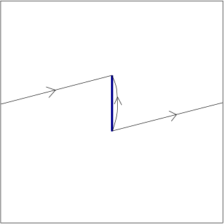
Figure 1: Open Wilson lines on a non-commutative torus admit longitudinal momenta, corresponding to translations all the way around the torus in a direction transverse to the Wilson line. The combination of longitudinal and transverse momenta must correspond to a translation relating the endpoints of the open Wilson line.

Similarly, we can construct the non-commutative duals of the $TrF^{2}(x)$ operators in the commutative theory using the explicit map between the gauge fields in the two theories . A straightforward calculation gives the following operator in terms of the Fourier modes of the field strength:

$$TrF^{2}(x)=N\sum_{k,n}f^{\mu\nu}_{Nk-n}f^{\mu\nu}_{n}e^{-\pi icNk_{1}k_{2}}e^{-\pi ic(n_{1}k_{2}-k_{1}n_{2})}e^{-\frac{i{\vec{k}}{\vec{x}}}{R}}.$$ (4.3.3)

In the non-commutative theory this yields a family of gauge invariant operators that depend explicitly on $N$. There is an obvious generalization to operators $TrF^{n}(x)$, which yield new gauge invariant operators in non-commutative gauge theories with rational non-commutativity parameter.

5 Continuity in $\Theta$

Continuity in $\Theta$ depends on the existence of very non-trivial relations between large and small $N$ gauge theories. For instance, if $\Theta=-1/2$, the commutative dual has $N=2$ and $m=1$, however if $\Theta=-1000/2001$ the commutative dual has $N=2001$ and $m=2$. Furthermore even at the classical level, the non-commutative theory on a torus does not have a manifestly smooth dependence on $\Theta$, since the gauge potential is periodic, with periodicity given by (3.1.17). Nevertheless, when considering gauge invariant observables we will find smooth dependence on $\Theta$, at least in the instances which we have thus far considered.

5.1 Energies

A first fairly trivial observation is that the BPS mass formulae in Yang-Mills theory [1, 7, 8, 9] with $16$ supercharges is consistent with continuity in $\Theta$. One can ask whether the same holds true for the energy of an electric flux line in a confining Yang-Mills theory. Consider the pure four-dimensional commutative Yang-Mills theory on the space $T^{2}\times S^{1}$ where the $S^{1}$ has size $L_{3}$ and the $\Theta$ parameter lives on the $T^{2}$ which has radii equal to $R$. For sufficiently large $R$, the principle contribution to the energy of an electric flux on $T^{2}$ comes from the confined flux lines in the $SU(N)/Z_{N}$ component of the theory. The energy of an electric flux $e_{i}$ is given by

$$E(e_{i})=\Lambda^{2}Re_{i}+\cdots.$$ (5.1.1)

where $\Lambda$ is the QCD scale and the omitted terms are subleading in $1/\Lambda R$. In the dual $U(1)$ non-commutative theory, this is the energy of a state created by an open Wilson line. For concreteness, consider an electric flux $e_{2}$. Continuity in $\Theta$ in the non-commutative theory implies that the energy of the electric flux can be written in terms of variables in the dual $U(1)$ non-commutative theory which vary smoothly or are fixed as one varies $\Theta$. Using formula (4.2.10) the energy of the commutative electric flux can be written as

$$E(e_{2})=\Lambda^{2}R^{\prime}(\frac{c}{N}n_{1}^{\prime}+{e}_{2}^{\prime})+\cdots.$$ (5.1.2)

Thus the energy is consistent with continuity in $\Theta=-c/N$ (at least to leading order in $1/\Lambda R$) provided the QCD scale $\Lambda$ can be written in terms of variables in the non-commutative dual which do not differ for arbitarily close values of $\Theta=-c/N$. In two-dimensional QCD, the string tension is $g^{2}N$ or ${g^{\prime}}^{2}$, which can indeed be held fixed as one varies $\Theta$. In four dimensions, we can address this question in the context of a confining vacuum of the ${\cal N}=1^{*}$ SYM theory. This theory is obtained by deforming the ${\cal N}=4$ theory with a mass term, which in ${\cal N}=1$ language adds $\Delta W=\frac{1}{g^{2}}MTrX^{2}$ to the superpotential. Morita equivalence treats the adjoint scalars in the same way as the gauge fields, so that the superpotential of the non-commutative dual is deformed by a term $\frac{1}{{g^{\prime}}^{2}}{M^{\prime}}{\cal X}^{2}$ with $M^{\prime}=M$. At very high energies, the ${\cal N}=1^{*}$ theory is conformal, with gauge coupling $g^{2}$ (in the commutative description), while below the scale $M$ the coupling runs according to the QCD beta-function. For small ’t Hooft coupling, the QCD scale is given by

$$\Lambda=Me^{-\frac{1}{g^{2}N}}$$ (5.1.3)

This can be written in terms of non-commutative variables as

$$\Lambda={M^{\prime}}e^{-\frac{1}{{g^{\prime}}^{2}}},$$ (5.1.4)

which is fixed as one varies $\Theta$.

At this stage we have only checked the continuity of energies in $\Theta$ to leading order in an $1/\Lambda R$ expansion. It may be that these results do not persist beyond leading order. For a very small torus, one could investigate the question of continuity in $\Theta$ perturbatively, but we shall not do so here.

5.2 Wilson loop correlators in ${\cal N}=4$ SYM.

Other quantities in the non-commutative theory which one might expect to depend smoothly on $\Theta$ are the correlation functions of open Wilson lines. We consider the correlation functions

$$G_{n_{1},e_{2}} \equiv <\hat{O}_{n_{1},e_{2}}\hat{O}_{-n_{1},-e_{2}}>$$

$$G^{\prime}_{n_{1}^{\prime},e_{2}^{\prime}} \equiv <\hat{O}^{\prime}_{n_{1}^{\prime},e_{2}^{\prime}}\hat{O}^{\prime}_{-n_{1}^{\prime},-e_{2}^{\prime}}>$$ (5.2.1)

of wrapped Wilson lines in the commutative theory and open Wilson lines in the non-commutative theory respectively. Via the duality map (4.2.9), continuity in $\Theta$ requires that the correlator of closed Wilson loops wrapping the torus in the commutative description has the following functional form

$$G_{n_{1},e_{2}}=\frac{1}{(2\pi RN)^{2}}G^{\prime}_{n_{1}^{\prime},e_{2}^{\prime}}=f(\Theta,{g^{\prime}}^{2},R^{\prime},n_{1}^{\prime},e_{2}^{\prime})=$$

$$f(-\frac{c}{N},g^{2}N,RN,Nn_{1}-me_{2},-cn_{1}+ae_{2})$$ (5.2.2)

Using $aN-cm=1$ and dimensional analysis, this can be rewritten as

$$G_{n_{1},e_{2}}=(e_{2}R)^{2}{\tilde{f}}(-\frac{c}{N},g^{2}N,Nn_{1}-me_{2},\frac{e_{2}}{N})$$ (5.2.3)

for some function $\tilde{f}$. Any other functional form would lead, via Morita equivalence, to a non-commutative theory in which the Wilson loop correlator differs between arbitarily close rational values of $\Theta$.

One could try to verify continuity perturbatively, since Morita equivalence is a classical duality. At leading order, the result for the correlator in the non-commutative theory is independent of $\Theta$ (see [20] ). Therefore, via Morita equivalence, the commutative theory has the right functional behavior at leading order (5.2.3). It would be interesting to check whether (5.2.3) is satisfied in a loop computation, although we will not do this here. In what follows, we shall verify the behavior predicted by continuity in $\Theta$ to leading order in the $1/N$ expansion of strongly coupled ${\cal N}=4$ $U(N)$ Yang-Mills theory.

Figure 2: A minimal surface connecting Wilson loops on the torus, depicted by a square with identified edges.

In the commutative ${\cal N}=4$ $U(N)$ Yang-Mills theory, the correlator of Wilson loops on $T^{2}$ can be computed at large $N$ and strong ’t Hooft coupling using the AdS-CFT correspondence [23, 24] and the method of [25] [26]. In this case one would at least expect that when a supergravity dual of the non-commutative theory exists (see [27, 28]), and the geometry depends smoothly on $\Theta$, the formula (5.2.3) ought to be satisfied. Note that the supergravity description is generically not valid in all T-dual descriptions of the theory (although there may be overlapping regions of validity). We shall look for the smooth behavior (5.2.3) directly in the supergravity description of the commutative theory. Consider the supergravity background which is dual to the commutative Yang-Mills theory with ’t Hooft flux $m$. The supergravity description is valid in the large $N$ limit at fixed but large ’t Hooft coupling. The background is given by

$$ds^{2} = \alpha^{\prime}\left[\frac{U^{2}}{\sqrt{\lambda}}(dt^{2}+dx_{1}^{2}+dx_{2}^{2}+dx_{3}^{2})+\frac{\sqrt{\lambda}dU^{2}}{U^{2}}+\sqrt{\lambda}d\Omega_{5}^{2}\right]$$

$$e^{\phi} = \frac{\lambda}{4\pi N}$$

$$B = -\frac{m}{N}\frac{1}{2\pi R^{2}}dx^{1}\wedge dx^{2}$$ (5.2.4)

where $\lambda=4\pi g^{2}N$ and $x^{1}$ and $x^{2}$ are compactified on a square torus of radius $R$. Note that the $B$ field takes precisely the value we imposed in section 3 to cancel the $U(1)$ flux. The correlator of Wilson loops can be obtained by summing over minimal area surfaces in $AdS_{5}\times S_{5}$ with boundaries given by the Wilson loops at the boundary of AdS space. Consider oppositely oriented Wilson loops wrapping the $2$-direction $e_{2}$ times at the points $x^{1}=x^{1}_{+}$ and $x^{1}_{-}$ as in figure 2.

The minimal area surfaces have the form

$$x^{2}(\sigma,\tau) = 2\pi Re_{2}\sigma$$

$$x^{1}(\sigma,\tau) = (x^{1}_{+}-x^{1}_{-}+2\pi Rn)\tau$$

$$U(\sigma,\tau) = U(\tau),$$ (5.2.5)

where $\sigma$ and $\tau$ are defined on the interval $[0,1]$ and $n$ is an integer characterizing the winding number of the minimal surface in the $x^{1}$ direction. $U(\tau)$ is determined by extremizing the world sheet action

$$S_{n}=\int\sqrt{detG}=2\pi Re_{2}\int d\tau\sqrt{\left(\frac{\partial U}{\partial\tau}\right)^{2}+\frac{U^{4}}{\lambda}\left|x^{1}_{+}-x^{1}_{-}+2\pi Rn\right|^{2}}.$$ (5.2.6)

Although the context is somewhat different, this is precisely the same minimization problem as the one solved in [26]. In the limit in which the boundaries are at $U\rightarrow\infty$, the world sheet action is divergent until making an appropriate subtraction. The result obtained after this subtraction can be extracted from [26] and is given by

$$S_{n}(x^{1}_{+}-x^{1}_{-})=-\frac{2\pi Re_{2}(4\pi)^{2}(2\lambda)^{1/2}}{\Gamma(\frac{1}{4})^{4}|x^{1}_{+}-x^{1}_{-}+2\pi Rn|}$$ (5.2.7)

In position space, the correlator of Wilson loops at strong ’t Hooft coupling and leading order in the $1/N$ expansion is given formally by

$$G_{e_{2}}(x^{1}_{+},x^{1}_{-})=e_{2}\sum_{n}\exp\left(-i\frac{me_{2}(x^{1}_{+}-x^{1}_{-}+2\pi Rn)}{NR}\right)\exp\left(-S_{n}(x^{1}_{+}-x^{1}_{-})\right)$$ (5.2.8)

Several comments are in order. First, the phase factor proportional to the magnetic flux arises because of the relation between the flux and the NS-NS B field modulus. Note that for $m=0\ mod\ N$, the sum on the index $n$ is divergent, due to the long range correlations of the ${\cal N}=4$ theory. We shall just consider the formal sum for the moment.

Second, the overall factor of $e_{2}$ in (5.2.8) requires some explanation. The Wilson loops forming the boundary of the minimal surface correspond to an element of the permutation group ${\cal S}_{e_{2}}$ which is a cycle of length $e_{2}$. The easiest way to understand the overall factor of $e_{2}$ in (5.2.8) is to infinitesimally deform both Wilson loops, so that the $e_{2}$ cycles of each do not lie on top of each other. For each Wilson loop, let us label the points at $x^{2}=0$ by an index $i\in\{1,\cdots,e_{2}\}$, and choose a point $i=1$ on one of the Wilson loops $\gamma^{-}$. As one follows the $x^{2}=0$ path on the world sheet from $\gamma^{-}$ to the other Wilson loop $\gamma^{+}$, there are $e_{2}$ possible end points on $\gamma^{+}$. These are topologically distinct when the boundaries are held fixed. One can also understand the factor of $e_{2}$ in terms of topologically distinct planar diagrams, as illustrated in figure 3. This factor of $e_{2}$ will prove essential for smooth dependence of the non-commutative dual on $\Theta$.

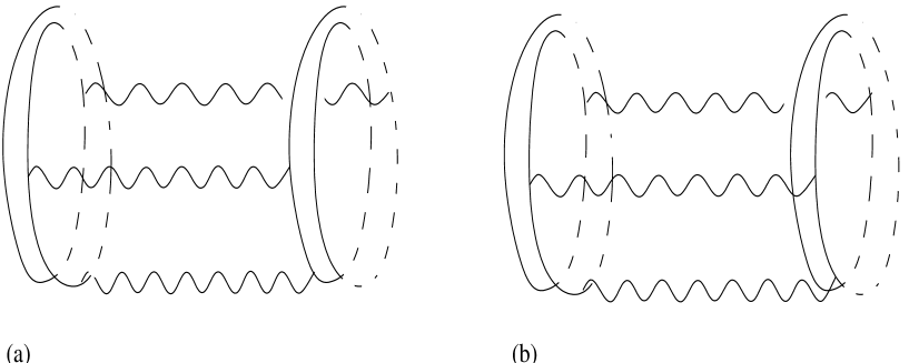
Figure 3: Two planar (ladder) diagrams giving an identical contribution to correlators of Wilson loops with $e_{2}=2$.

Note that due to the sum on $n$ in (5.2.8), the correlator is periodic in $x^{1}_{+}$ and $x^{1}_{-}$. Recall that the $SU(N)$ Wilson loop defined by (4.1.4) is not periodic in the presence of ’t Hooft flux [21], whereas the $U(N)$ Wilson loop is periodic. In the commutative case, the AdS-CFT relation is said to describe an $SU(N)/Z_{N}$ rather than $U(N)$ theory (e.g. [24]). We therefore interpret the result (5.2.8) as the correlator of $U(N)$ Wilson loops with a non-dynamical background $U(1)$, with first Chern class equal to the $SU(N)$ ’t Hooft flux. We now Fourier transform (5.2.8), giving the correlator of Wilson loops with momentum $n_{1}$:

$$G_{n_{1},e_{2}} = \int_{0}^{2\pi R}dx^{1}_{+}\int_{0}^{2\pi R}dx^{1}_{-}e^{i\frac{n_{1}(x^{1}_{+}-x^{1}_{-})y}{R}}G_{e_{2}}(x^{1}_{+},x^{1}_{-})$$

$$= 2\pi Re_{2}\int_{0}^{2\pi R}dy\exp(i\frac{n_{1}y}{R})$$

$$\sum_{n=-\infty}^{+\infty}\exp\left(-i\frac{me_{2}(y+2\pi Rn)}{NR}\right)\exp\left(\frac{2\pi Re_{2}(4\pi)^{2}(2\lambda)^{1/2}}{\Gamma(\frac{1}{4})^{4}|y+2\pi Rn|}\right)$$

$$= 2\pi Re_{2}\int_{-\infty}^{+\infty}dy\exp\left(i\frac{(n_{1}N-me_{2})y}{NR}\right)\exp\left(\frac{2\pi Re_{2}(4\pi)^{2}(2\lambda)^{1/2}}{\Gamma(\frac{1}{4})^{4}|y|}\right)$$

Note that this converges as long as the momentum $n_{1}N-me_{2}$ is non-zero. The zero momentum divergence arises because the ${\cal N}=4$ theory is conformal. The correlator (5.2) has the functional form

$$G_{n_{1},e_{2}}=(e_{2}R)^{2}f(g^{2}N,(n_{1}N-me_{2})\frac{e_{2}}{N})$$ (5.2.10)

which is consistent with continuity in $\Theta$. It would be very interesting to explicitly see if the $\frac{1}{N}$ corrections are also consistent with continuity in $\Theta$. Very little is known about the $1/N$ corrections in the strongly coupled ${\cal N}=4$ super Yang-Mills theory. Still, the behavior of the leading term in the large $N$ result is by itself non-trivial.

Note that one expects the Wilson loop correlator in the commutative theory to depend smoothly on $m/N$ in ’t Hooft large $N$ limit at fixed $e_{2}$, $n_{1}$ and $R$. This excludes explicit dependence on $-c/N$ in the $1/N$ expansion. Assuming this and continuity in $\Theta$ implies a $1/N$ expansion of the form

$$G_{n_{1},e_{2}}=(Re_{2})^{2}\sum_{l}\left(\frac{e_{2}}{N}\right)^{l}g_{l}\left(g^{2}N,\frac{e_{2}}{N}(Nn_{1}-me_{2})\right)$$ (5.2.11)

In writing this expression we have also made use of the fact that $Nn_{1}-me_{2}$ grows like $N$ for a generic choice of $n_{1}$ and $e_{2}$, while the argument of $g_{l}$ is by definition of order one.

The above discussion has some interesting consequences for gauge theory on a non-commutative $R^{2}$ in the $\theta\rightarrow\infty$ limit. It has been pointed out that the $\theta\rightarrow\infty$ limit of a field theory on a non-commutative $R^{2}$ behaves like a string theory, due to the vanishing of all but the planar graphs [29]. In the $N\rightarrow\infty$ limit of the commutative theory with $R,e_{2},n_{1}$ and $m/N$ fixed, the correlator (5.2) can be interpreted as that of an open Wilson line with fixed length and transverse momentum in the strong coupling limit of the $\theta\rightarrow\infty$ theory, where $\theta=\Theta 2\pi{R^{\prime}}^{2}$ and $R^{\prime}=RN\rightarrow\infty$. The length of the open Wilson line is

$$L^{\prime}=\Theta n_{1}^{\prime}+2\pi R^{\prime}e_{2}^{\prime}=e_{2}R$$ (5.2.12)

while the momentum is

$$p^{\prime}=\frac{n_{1}^{\prime}}{R^{\prime}}=\frac{(Nn_{1}-me_{2})}{NR},$$ (5.2.13)

both of which are fixed in the large $N$ limit. It may seem odd that open Wilson lines of arbitrary momentum $p$ and length $L$ exist in the infinite $\theta$ and infinite $R^{\prime}$ limit of the non-commutative theory, where one would naively write $L^{\prime}=\theta p^{\prime}$. However the non-commutative electric flux $e_{2}^{\prime}$ can conspire to give a finite length in this limit, since the length is actually given by (5.2.12).

5.3 Wilson loop correlators in confining Yang-Mills

The Morita equivalence (4.2.9) applies classically even in the pure $U(N)$ Yang-Mills theory. This raises the question of whether confining Yang-Mills theories exhibit behavior consistent with continuity in $\Theta$. These theories differ greatly from the ${\cal N}=4$ theory, and in the non-commutative case exhibit $UV/IR$ mixing [29]. Furthermore, it is difficult to embed asymptotically free confining theories in string theory. It may be that the ${\cal N}=4$ case exhibits continuity in $\Theta$ while the confining theories do not. We shall address this question of continuity in $\Theta$ in the $1/N$ expansion of confining Yang-Mills and find evidence for continuity at leading order.

Based in large part on observations of ’t Hooft [30], the large $N$ limit of QCD is expected to be described by a string theory. In two dimensions, where an exact solution exists [31], the string description has been constructed [32, 33, 34, 35, 36, 37]. Let us consider this situation first. We will again consider the correlation function of Wilson loops $\hat{O}_{n_{1},e_{2}}$ wrapping the torus. The correlator can be computed using methods described in [35, 36]. The basic idea is that one sums over maps without folds from the world sheet to the target space, $\Sigma\rightarrow T$, such that the boundary $\partial\Sigma$ is a cyclic $e_{2}$-fold cover of the $S^{1}$ associated to each Wilson loop. At leading order in the $1/N$ expansion, one sums over covers without branch points. The ’t Hooft magnetic flux plays the role of a $B$ field modulus of the 2-d QCD string. This means that in the sum over maps of the worldsheet to the target space $\Sigma\rightarrow T$, string worldsheets are weighted by a phase factor

$$e^{-i\frac{m}{N}\frac{1}{2\pi R^{2}}\int_{\Sigma}dx^{1}\wedge dx^{2}}$$ (5.3.1)

just as in the AdS-CFT case. In 2-d QCD this can be seen for instance by computing with the heat kernel action with twisted boundary conditions. The correlation function at leading order in $1/N$ is given by

$$G_{n_{1},e_{2}} = 2\pi Re_{2}\int_{0}^{2\pi R}dy\exp(i\frac{n_{1}y}{R})$$ (5.3.2)

$$\sum_{n=-\infty}^{+\infty}\exp\left(-i\frac{me_{2}(y+2\pi Rn)}{NR}\right)\exp\left(-\lambda 2\pi Re_{2}|y+2\pi Rn|\right)$$

where $\lambda$ is the ’t Hooft coupling $g^{2}N$ and $n$ indicates a winding number of the world sheet in the direction transverse to the Wilson loops. The overall factor of $e_{2}$ arises for the same reasons as in the AdS-CFT case. The above expression can be rewritten as

$$G_{n_{1},e_{2}}=2\pi Re_{2}\int_{-\infty}^{\infty}dy\exp(i\frac{(n_{1}N-me_{2})y}{NR})\exp\left(-\lambda 2\pi Re_{2}|y|\right)$$ (5.3.3)

This is manifestly consistent with smooth dependence on $\Theta$, as it depends only on the variables $e_{2}R,g^{2}N,NR$ and $n_{1}N-me_{2}$. At this point we have been somewhat cavalier about the distinction between $U(N)$ and $SU(N)$. The above correlator is that of an $SU(N)$ Wilson loop, with an extra $U(1)$ phase factor in the transition function such that the Wilson loop is periodic in the transverse direction. This can be interpreted as a $U(N)$ correlator with a frozen $U(1)$, much like the correlator in the AdS-CFT case. At higher orders in the $1/N$ expansion, the distinction between $U(N)$ and $SU(N)$ will certainly be important. The role of the $U(1)$ is at this stage somewhat mysterious. It would be interesting to compute the $1/N$ corrections, and see if they are consistent with continuity in $\Theta$. The $1/N$ corrections arise by considering branched covers, as well as collapsed handles and tubes in the $SU(N)$ case.

One can also make similar statements about continuity in $\Theta$ in four dimensional confining Yang-Mills theories. The argument depends crucially on the relation of the ’t Hooft magnetic flux to a B field modulus of the 4-d QCD string. This relation can be shown [39] in the context of MQCD [40] and its IIA limit where it arises as a consequence of a freezing of the $U(1)$ degree of freedom. In the MQCD context, the correlator can be computed by summing over M2-branes with boundaries on the Wilson loop times an interval (see [39] ). At leading order the result is identical to (5.3.3) with the replacement $\lambda\rightarrow\Lambda^{2}$, where $\Lambda^{2}$ is the MQCD string tension.

6 Conclusions and discussion

The existence of renormalizable gauge theories on non-commutative spaces is still an open question. For rational $\Theta$, the theory may be defined on the torus via Morita equivalence with gauge theory on a commutative torus. However it is not manifest that observable quantities are arbitrarily close for arbitrarily close values of $\Theta$, as one would require to define the theory for irrational $\Theta$. For this to be the case, there must be strong constraints on observables in commutative Yang-Mills theories. In other words, if the non-commutative gauge theory on the torus could be defined for all values of $\Theta$, consistent with Morita equivalence, we would have strong predictions for commutative gauge theories on tori.

The strong constraints on commutative gauge theories are easily seen to be satisfied for such quantities as the energies of BPS states in Yang-Mills theories with $16$ supercharges. In this paper we have verified that these constraints are also obeyed by the correlator of wrapped Wilson loops, to leading order in the $1/N$ expansion of four dimensional ${\cal N}=4$ Yang-Mills theory, and pure two dimensional QCD. We also presented rough arguments concerning the behavior of this correlator in confining four dimensional QCD, where it again seems to be consistent with continuity in $\Theta$.

While the leading $1/N$ behavior of the correlator is consistent with continuity in $\Theta$, there exist other quantities which do not vary continuously with $\Theta$. Amongst these is the periodicity of the non-commutative gauge potential, and certain observables which can only be defined for rational values of $\Theta$. Moreover, in the two-dimensional case, continuity in $\Theta$ is only exhibited by the correlator, but not by the partition function.

To check further whether commutative gauge theories satisfy the constraints implied by smooth non-commutative duals, it would be enlightening to study the subleading terms in the $1/N$ expansion in cases in which this is possible, such as two-dimensional QCD. Perhaps a next to leading order term can shed light on whether the pattern observed in this paper persists. If it persists, it yields strong predictions on commutative gauge theories. If it does not, there is a puzzle as to the definition of non-commutative gauge theories on the torus for irrational values of $\Theta$. It would also be interesting to check continuity in $\Theta$ perturbatively. In the confining case, this can be done on a sufficiently small torus.

A further point of investigation could be the following. Using the AdS/CFT correspondence, we computed the correlator of closed Wilson loops in the large $N$ limit. We made good use of the fact that the correlator of spatially separated Wilson loops is equivalent to a computation of the quark-anti-quark potential with a compactified time direction (where the compactification is assumed to preserve supersymmetry). That allowed us to recuperate the results in [26]. We expect this correlator to be equivalent to a correlator of open Wilson lines in a non-commutative $U(p)$ theory that we should be able to compute at large $p$ using the non-commutative version of the AdS/CFT correspondence [41, 42]. Since these correlators are dual, they should yield the same result, after dualising momentum and winding number of the loops. It should be instructive to try and follow the AdS/CFT correspondence (for theories compactified on tori) under the Morita equivalence map, to learn more about the correspondence for non-commutative field theories.

7 Appendix: mapping Wilson lines

In this appendix we prove the relation (4.2.9) discussed in [11, 12], taking into account Wilson lines with both winding and transverse momentum. We will do so by expanding the path ordered exponentials in $\hat{O}^{\prime}_{n_{1}^{\prime},e_{2}^{\prime}}$ and $2\pi RN\hat{O}_{n_{1},e_{2}}$ as follows:

$$P(e^{i\int A})=\ \ \ \ \ \ \ \ \ \ \ \ \ \ \ \ \ \ \ \ \ \ \ \ \ \ \ \ \ \ \ \ \ \ \ \ \ \ \ \ \ \ \ \ \ \ \ \ \ \ \ \ \ \ \ \ \ \ \ \ \ \ \ \ \ \ \ \ \ \ \ \ \ \ \ \ \ \ \ \ \ \ \ \ \ \ \$$

$$1+i\int_{0}^{1}dsA_{\mu}(x(s))\frac{dx^{\mu}(s)}{ds}-\int_{0}^{1}ds\int_{0}^{s}d{\tilde{s}}A_{\mu}(x(s))A_{\nu}(x({\tilde{s}}))\frac{dx^{\mu}(s)}{ds}\frac{dx^{\nu}(\tilde{s})}{d\tilde{s}}+\cdots$$

(7.1)

and showing equivalence at all orders. Inserting this expansion into the expression (4.2.7) for the operator $2\pi RN\hat{O}$, and using expression (3.1.8) for $A$, gives

$$\int_{0}^{2\pi R}dx^{1}\int_{0}^{1}ds_{a}\int_{0}^{s_{a}}ds_{b}\cdots\exp\left(-2\pi i(r_{2a}s_{a}+r_{2b}s_{b}+\cdots)\frac{e_{2}}{N}\right)$$

$$\exp\left(-i\pi\frac{c}{N}(r_{1a}r_{2a}+r_{1b}r_{2b}+\cdots)\right)Tr\left(Q^{-cr_{1a}}P^{r_{2a}}Q^{-cr_{1b}}P^{r_{2b}}\cdots Q^{-e_{2}}\right)$$

$$\exp\left(-i(\vec{r}_{a}\cdot\vec{x}+\vec{r}_{b}\cdot\vec{x}\cdots+me_{2}x^{1})/NR\right)\exp(in_{1}x^{1}/R)a^{2}_{\vec{r}_{a}}a^{2}_{\vec{r}_{b}}\cdots$$

$$2\pi RN(2\pi Re_{2})^{k}$$ (7.2)

where we have used

$$x^{2}(s)=x^{2}+2\pi Re_{2}s$$ (7.3)

for $s$ defined on the interval $[0,1]$ and $k$ denotes the order in the expansion of the exponential. We wish to show that (7.2) is equivalent order by order to the analogous expansion for $\hat{O}$, given by

$$\int_{0}^{2\pi R^{\prime}}dx^{1}\int_{0}^{2\pi R^{\prime}}dx^{2}\int_{0}^{1}ds_{a}\int_{0}^{s_{a}}ds_{b}\cdots$$

$$\exp\left(-2\pi i(r_{2a}s_{a}+r_{2b}s_{b}+\cdots)(e_{2}^{\prime}+\frac{c}{N}n_{1}^{\prime})\right)$$

$$\exp\left(-i\frac{(\vec{r}_{a}\cdot\vec{x})}{R^{\prime}}\right)*\exp\left(-i\frac{(\vec{r}_{b}\cdot\vec{x})}{R^{\prime}}\right)\cdots$$

$$\exp\left(i\frac{n_{1}^{\prime}x^{1}}{R^{\prime}}\right)a^{2}_{\vec{r}_{a}}a^{2}_{\vec{r}_{b}}\cdots\left(2\pi R^{\prime}(e_{2}^{\prime}+\frac{c}{N}n_{1}^{\prime})\right)^{k}$$

(7.4)

We will begin with (7.2) and reorder the quantities within the trace, giving

$$Tr\left(Q^{-cr_{1a}}P^{r_{2a}}Q^{-cr_{1b}}P^{r_{2b}}\cdots Q^{-e_{2}}\right) =$$

$$Tr\left(Q^{-cr_{1a}-cr_{1b}+\cdots-e_{2}}P^{r_{2a}+r_{2b}+\cdots}\right)\phi(\vec{r}_{a},\vec{r}_{b}\cdots,me_{2})$$ (7.5)

where $\phi$ is a $Z_{N}$ phase. It will not be necessary to write it explicitly. Now one can readily verify that the quantity

$$Tr\left(Q^{-cr_{1a}-cr_{1b}+\cdots-e_{2}}P^{r_{2a}+r_{2b}+\cdots}\right)$$ (7.6)

vanishes unless

$$-c(r_{1a}+r_{1b}+\cdots-me_{2})=kN$$ (7.7)

and

$$-c(r_{2a}+r_{2b}+\cdots)=jN$$ (7.8)

for integers $k$ and $j$. If these conditions are satisfied then, since $P^{N}=Q^{N}=1$,

$$Tr\left(Q^{-cr_{1a}-cr_{1b}+\cdots-e_{2}}P^{r_{2a}+r_{2b}+\cdots}\right)=N$$ (7.9)

The Wilson loop is independent of the base point $x^{2}$, so all contributions from non-zero $j$ vanish.

Let us now consider the integral over the $x^{1}$ dependent parts of (7.2),

$$\int dx^{1}\exp\left(-i\frac{(r_{1a}+r_{1b}+\cdots+me_{2}-n_{1}N)x^{1}}{NR}\right).$$ (7.10)

Since $gcd(N,c)=1$ via (3.1.7), we can rewrite (7.7) as

$$r_{1a}+r_{1b}+\cdots-me_{2}=qN$$ (7.11)

where $q$ is an integer. Therefore (7.10) is an integral over a periodic function, giving

$$2\pi R\delta_{0,r_{1a}+r_{1b}+\cdots+me_{2}-n_{1}N}$$ (7.12)

We can therefore write (7.2) as

$$\int_{0}^{2\pi R}dx^{1}\int_{0}^{2\pi R}dx^{2}\int_{0}^{1}ds_{a}\int_{0}^{s_{a}}ds_{b}\cdots\exp\left(-2\pi i(r_{2a}s_{a}+r_{2b}s_{b}+\cdots)\frac{e_{2}}{N}\right)$$

$$\exp\left(-i\pi\frac{c}{N}(r_{1a}r_{2a}+r_{1b}r_{2b}+\cdots)\right)\exp\left(-i\frac{(r_{1a}+r_{1b}+\cdots+me_{2}-n_{1}N)x^{1}}{R}\right)$$

$$\exp\left(i\frac{(r_{2a}+r_{2b}+\cdots)x^{2}}{R}\right)\phi(\vec{r}_{a},\vec{r}_{b}\cdots,me_{2})a^{2}_{\vec{r}_{a}}a^{2}_{\vec{r}_{b}}\cdots\frac{N}{2\pi R}2\pi RN(2\pi Re_{2})^{k}$$

(7.13)

This expression is equivalent to the following integral over the non-commutative torus;

$$\int_{0}^{2\pi R^{\prime}}dx^{1}\int_{0}^{2\pi R^{\prime}}dx^{2}\int_{0}^{1}ds_{a}\int_{0}^{s_{a}}ds_{b}\cdots\exp\left(-2\pi i(r_{2a}s_{a}+r_{2b}s_{b}+\cdots)\frac{e_{2}}{N}\right)$$

$$\exp\left(-i\pi\frac{c}{N}(r_{1a}r_{2a}+r_{1b}r_{2b}+\cdots)\right)\exp\left(i\frac{(r_{1a}+r_{1b}+\cdots+me_{2}-n_{1}N)x^{1}}{R^{\prime}}\right)*$$

$$\exp\left(-i\frac{(r_{2a}+r_{2b}+\cdots)x^{2}}{R^{\prime}}\right)$$

$$\phi(\vec{r}_{a},\vec{r}_{b}\cdots,me_{2})a^{2}_{\vec{r}_{a}}a^{2}_{\vec{r}_{b}}\cdots(2\pi Re_{2})^{k}$$

(7.14)

where we have used $R^{\prime}=RN$ and the fact that $\int d^{2}x\,A*B=\int d^{2}x\,A.B$. We can now make use of a relation between the $\ast$-algebra and the matrix algebra generated by $Q$ and $P$. Note that

$$Q^{-cr_{1}}P^{r_{2}}=P^{r_{2}}Q^{-cr_{1}}\exp(2\pi i\frac{c}{N}r_{1}r_{2})$$ (7.15)

and

$$\exp(-i\frac{r_{1}x^{1}}{R^{\prime}})*\exp(-i\frac{r_{2}x^{2}}{R^{\prime}})=$$

$$\exp(-i\frac{r_{2}x^{2}}{R^{\prime}})*\exp(-i\frac{r_{1}x^{1}}{R^{\prime}})\exp(2\pi i\frac{c}{N}r_{1}r_{2})$$ (7.16)

Thus

$$\exp\left(-i\frac{r_{1a}x^{1}}{R^{\prime}}\right)*exp\left(-i\frac{r_{2a}x^{2}}{R^{\prime}}\right)*exp\left(-i\frac{r_{1b}x^{1}}{R^{\prime}}\right)*exp\left(-i\frac{r_{2b}x^{2}}{R^{\prime}}\right)*\cdots$$

$$\exp\left(-i\frac{me_{2}x^{1}}{R^{\prime}}\right)=$$

$$\exp\left(-i\frac{(r_{1a}+r_{1b}+\cdots+me_{2}-n_{1}N)x^{1}}{R^{\prime}}\right)*\exp\left(-i\frac{(r_{1a}+r_{1b}+\cdots)x^{2}}{R^{\prime}}\right)$$

$$\phi(\vec{r}_{a},\vec{r}_{b},\cdots,me_{2})$$

(7.17)

where, since $Q^{-e_{2}}=Q^{-cme_{2}}$, the phase $\phi$ in (7.17) is the same as that which appears in (7.5). Furthermore we have

$$\exp\left(-i\frac{r_{1}x^{1}}{R^{\prime}}\right)*exp\left(-i\frac{r_{2}x^{2}}{R^{\prime}}\right)=\exp\left(-i\frac{\vec{r}\cdot\vec{x}}{R^{\prime}}\right)\exp\left(i\frac{c}{N}\pi r_{1}r_{2}\right).$$ (7.18)

Therefore (7.14) may be written as

$$\int_{0}^{2\pi R^{\prime}}dx^{1}\int_{0}^{2\pi R^{\prime}}dx^{2}\int_{0}^{1}ds_{a}\int_{0}^{s_{a}}ds_{b}\cdots\exp\left(-2\pi i(r_{2a}s_{a}+r_{2b}s_{b}+\cdots)\frac{e_{2}}{N}\right)$$

$$\exp\left(-i\frac{\vec{r}_{a}\cdot\vec{x}}{R^{\prime}}\right)*\exp\left(-i\frac{\vec{r}_{b}\cdot\vec{x}}{R^{\prime}}\right)\cdots*\exp\left(-i\frac{(me_{2}-n_{1}N)x^{1}}{R^{\prime}}\right)$$

$$a^{2}_{\vec{r}_{a}}a^{2}_{\vec{r}_{b}}\cdots(2\pi Re_{2})^{k}$$

(7.19)

Formula (7.19) is now identical to (7.4) with the identification

$$\pmatrix{e_{2}^{\prime}\cr n_{1}^{\prime}}=\pmatrix{a&-c\cr-m&N}\pmatrix{e_{2}\cr n_{1}}$$ (7.20)

This completes the proof.

References

- [1] A. Connes, M. Douglas, and A. Schwarz, Noncommutative Geometry and Matrix Theory: Compactification on Tori, JHEP 9802 (1998) 003, hep-th/9711162.
- [2] N. Seiberg and E. Witten, String Theory and Noncommutative Geometry, JHEP 9909 (1999) 032, hep-th/9908142.
- [3] A. Schwarz, Morita equivalence and duality, Nucl. Phys. B 534 (1998) 720, hep-th/9805034.
- [4] S. Elitzur, B. Pioline and E. Rabinovici, On the short-distance structure of irrational noncommutative gauge theories, JHEP0010 (2000) 011. hep-th/0009009.
- [5] A. Hashimoto and N. Itzhaki, On the hierarchy between noncommutative and ordinary supersymmetric Yang-Mills, JHEP9912 (1999) 007, hep-th/9911057.
- [6] A. Konechny and A. Schwarz, Moduli spaces of maximally supersymmetric solutions on noncommutative tori and noncommutative orbifolds, JHEP0009 (2000) 005, hep-th/0005174.
- [7] C. Hofman and E. Verlinde, Gauge bundles and Born-Infeld on the noncommutative torus, Nucl. Phys. B 547 (1999) 157, hep-th/9810219.
- [8] A. Konechny and A. Schwarz BPS states on noncommutative tori and duality, Nucl. Phys. B 550, (1999) 561, hep-th/9811159.
- [9] B. Pioline and A. Schwarz, Morita Equivalence and T Duality (or B versus Theta), JHEP 9908(1999) 021, hep-th/9908019.
- [10] D. Bigatti, Noncommutative Geometry and Super Yang-Mills Theory, Phys. Lett.B451 (1999) 324, hep-th/9804120
- [11] J. Ambjorn, Y. M. Makeenko, J. Nishimura and R. J. Szabo, Lattice gauge fields and discrete noncommutative Yang-Mills theory, JHEP0005, (2000) 023, hep-th/0004147.
- [12] K. Saraikin, Comments on the Morita equivalence, J. Exp. Theor. Phys. 91, 653 (2000) hep-th/0005138.
- [13] T. Filk, Divergencies in a field theory on quantum space, Phys. Lett. B 376, (1996) 53, and references thereto.
- [14] D. Brace, B. Morariu and B. Zumino, Dualities of the matrix model from T-duality of the type II string, Nucl. Phys. B 545, 192 (1999), hep-th/9810099; D. Brace, B. Morariu and B. Zumino, T-duality and Ramond-Ramond backgrounds in the matrix model, Nucl. Phys. B 549, 181 (1999), hep-th/9811213.
- [15] Z. Guralnik, Duality of large N Yang-Mills theory on , hep-th/9804057.
- [16] G. ’t Hooft, A Property of Electric and Magnetic Flux in Nonabelian Gauge Theories, Nucl.Phys.B153 (1979) 141.
- [17] Z. Guralnik and S. Ramgoolam, Torons and D-brane bound states, Nucl. Phys. B 499, 241 (1997), hep-th/9702099.
- [18] N. Ishibashi, S. Iso, H. Kawai and Y. Kitazawa, Wilson loops in noncommutative Yang-Mills, Nucl. Phys. B 573 (2000) 573, hep-th/9910004.
- [19] S. Rey and R. von Unge, S-duality, noncritical open string and noncommutative gauge theory, Phys. Lett. B 499, 215 (2001), hep-th/0007089; S. R. Das and S. Rey, Open Wilson lines in noncommutative gauge theory and tomography of holographic dual supergravity, Nucl. Phys. B 590, 453 (2000), hep-th/0008042; S. R. Das and S. P. Trivedi, Supergravity couplings to noncommutative branes, open Wilson lines and generalized star products, JHEP0102, 046 (2001), hep-th/0011131.
- [20] D. Gross, A. Hashimoto and N. Itzhaki, Observables of Noncommutative Gauge Theories, hep-th/0008075.
- [21] P. van Baal, QCD in a Finite Volume, Boris Ioffe Festschrift, ed. by M. Shifman, World Scientific, hep-ph/0008206, and references therein.
- [22] L. G. Yaffe and B. Svetitsky, First Order Phase Transition In The SU(3) Gauge Theory At Finite Temperature, Phys. Rev. D 26, (1982) 963.
- [23] J. Maldacena, The large N limit of superconformal field theories and supergravity, Adv. Theor. Math. Phys. 2, 231 (1998), hep-th/9711200; S. S. Gubser, I. R. Klebanov and A. M. Polyakov, Gauge theory correlators from non-critical string theory, Phys. Lett. B 428, 105 (1998), hep-th/9802109.
- [24] E. Witten, Anti-de Sitter space and holography, Adv. Theor. Math. Phys. 2 (1998) 253, hep-th/9802150.
- [25] S. Rey and J. Yee, Macroscopic strings as heavy quarks in large N gauge theory and anti-de Sitter supergravity, hep-th/9803001; S. Rey, S. Theisen and J. Yee, Wilson-Polyakov loop at finite temperature in large N gauge theory and anti-de Sitter supergravity, Nucl. Phys. B 527, 171 (1998), hep-th/9803135.
- [26] J. Maldacena, Wilson loops in large N field theories, Phys. Rev. Lett. 80, (1998) 4859, hep-th/9803002
- [27] A. Hashimoto and N. Itzhaki, Noncommutative Yang-Mills and the AdS/CFT correspondence, Phys. Lett. B 465, (1999) 142, hep-th/9907166.
- [28] J. M. Maldacena and J. G. Russo, Large N limit of noncommutative gauge theories, JHEP9909, (1999) 025, hep-th/9908134.
- [29] S. Minwalla, M.V. Raamsdonk and N. Seiberg, Noncommutative Perturbative Dynamics, JHEP0002 (2000) 020, hep-th/9912072.
- [30] G. ’t Hooft, A Planar Diagram Theory For Strong Interactions, Nucl. Phys. B 72 (1974) 461.
- [31] B. E. Rusakov, Loop Averages And Partition Functions In U(N) Gauge Theory On Two-Dimensional Manifolds, Mod. Phys. Lett. A 5 (1990) 693.
- [32] V. A. Kazakov and I. K. Kostov, Nonlinear Strings In Two-Dimensional U(Infinity) Gauge Theory, Nucl. Phys. B 176 (1980) 199.
- [33] D. J. Gross, Two-dimensional QCD as a string theory, Nucl. Phys. B 400 (1993) 161, hep-th/9212149.
- [34] D. Gross and W. Taylor, Two-dimensional QCD is a string theory, Nucl. Phys. B 400 (1993) 181, hep-th/9301068.
- [35] D. Gross and W. Taylor, Twists and Wilson loops in the string theory of two-dimensional QCD, Nucl. Phys. B 403 (1993) 395, hep-th/9303046.
- [36] S. Cordes, G. Moore and S. Ramgoolam, Large N 2-D Yang-Mills theory and topological string theory, Commun. Math. Phys. 185 (1997) 543, hep-th/9402107.
- [37] P. Horava, Topological rigid string theory and two-dimensional QCD, Nucl. Phys. B 463 (1996) 238. hep-th/9507060.
- [38] Z. Guralnik, T-duality of large N QCD, hep-th/9903021.
- [39] Z. Guralnik, Strings and discrete fluxes of QCD, JHEP0003, (2000) 003, hep-th/9903014.
- [40] E. Witten, Branes and the dynamics of QCD, Nucl. Phys. B 507 (1997) 658, proceeding of Paris 1998, Quantum chromodynamics, 201-207, hep-th/9706109.
- [41] M. Alishahiha, Y. Oz and M. M. Sheikh-Jabbari, Supergravity and large N noncommutative field theories, JHEP9911 (1999) 007, hep-th/9909215.
- [42] A. Dhar and Y. Kitazawa, Wilson loops in strongly coupled noncommutative gauge theories, hep-th/0010256.