Vacuum structure of spontaneously broken
${\cal N}=2$ supersymmetric gauge theory

Abstract
We analyze the vacuum structure of spontaneously broken ${\cal N}=2$ supersymmetric gauge theory with the Fayet-Iliopoulos term. Our theory is based on the gauge group $SU(2)\times U(1)$ with $N_{f}=1,2$ massless quark hypermultiplets having the same $U(1)$ charges. In the classical potential, there are degenerate vacua even in the absence of supersymmetry. It is shown that this vacuum degeneracy is smoothed out, once quantum corrections are taken into account. In $N_{f}=1$ case, the effective potential is found to be so-called runaway type, and there is neither well-defined vacuum nor local minimum. On the other hand, in $N_{f}=2$ case, while there is also the runaway direction in the effective potential, we find the possibility that there appears the local minimum with broken supersymmetry at the degenerate dyon point.

I Introduction

There has been much progress in understanding the dynamics of strongly coupled ${\cal N}=1,2$ supersymmetric (SUSY) gauge theories. The exact effective superpotential can be derived for ${\cal N}=1$ SUSY QCD (SQCD) by using holomorphy properties of the superpotential and the gauge kinetic function [1]. Seiberg and Witten derived the exact low energy Wilsonian effective action for ${\cal N}=2$ SUSY $SU(2)$ Yang-Mills theory [2], and generalized their discussion to the case with up to four massive quark hypermultiplets [3]. The key ingredients which allow us to derive the exact results are duality and holomorphy. One can write down the prepotential and the gauge couplings in terms of the meromorphic differential on the Riemann surface with genus one whose properties are determined by the dynamical scale and the hypermultiplet masses.

The results by Seiberg and Witten were extended to the case with the explicit soft SUSY breaking terms by using the spurion technique. Unless these terms do not change the holomorphy and duality properties of the theory, we can derive the exact effective action for ${\cal N}=1$ and ${\cal N}=0$ (non-supersymmetric) SUSY gauge theories up to the leading order for the soft SUSY breaking terms. In Refs. [4, 5], the exact superpotential and the phase structure in ${\cal N}=1$ SQCD were discussed based on the ${\cal N}=2$ SUSY gauge theory with some soft breaking terms. In Refs. [6, 7, 8], the vacuum structure of non-SUSY gauge theory was investigated in which soft SUSY breaking terms directly break ${\cal N}=2$ SUSY to ${\cal N}$=0. As further extensions, the method to introduce non-holomorphic soft SUSY breaking terms was recently discussed [9].

In this paper, we study a spontaneously broken ${\cal N}=2$ SUSY gauge theory. It is well known that, in the framework of ${\cal N}=2$ SUSY theory, the only possibility to break SUSY spontaneously is to introduce the Fayet-Iliopoulos (FI) term [10]. Therefore, in the following, we consider the gauge theory which includes $U(1)$ gauge interaction together with the FI term.

The simplest example of this type of theory is ${\cal N}=2$ SUSY QED (SQED) with the FI term [11]. At the classical level, although SUSY is spontaneously broken in Coulomb branch, there are degenerate vacua (moduli space) which are parameterized by the vacuum expectation value of the scalar field, $a$, in the $U(1)$ vectormultiplet. The direction of this vacuum degeneracy in the absence of SUSY is called “pseudo flat” direction. However, it is expected that this direction is lifted up, once quantum corrections are taken into account. By virtue of ${\cal N}=2$ SUSY, the effective action is found to be one loop exact, and the effective gauge coupling is given by $e(a)^{2}\sim 1/\log(\Lambda_{L}/a)$, where $\Lambda_{L}$ is the Landau pole. Note that there are two singular regions in moduli space, namely, the ultraviolet region such as $|a|\geq\Lambda_{L}$, and the massless singular point at the origin $a=0$. Since the effective potential is described as $V\sim e(a)^{2}$, the potential minimum emerges at the origin, where SUSY is formally restored. However, since this point is the singular point, we conclude that there is no well-defined vacuum in this theory.

In this paper, we investigate the vacuum structure of more interesting theory with spontaneous ${\cal N}=2$ SUSY breaking. Our theory is based on the gauge group $SU(2)\times U(1)$ with $N_{f}=1,2$ massless quark hypermultiplets having the same $U(1)$ charges. In the ultraviolet region, the behavior of the effective potential can be well understood based on the perturbative discussion, since the $SU(2)$ gauge interaction is weak there. On the other hand, it is expected that the behavior of the effective potential in the infrared region is drastically changed compared with SQED, because of the presence of the $SU(2)$ gauge dynamics.

The paper is organized as follows. In the next section, we briefly discuss the classical structure of our theory. It is shown that the classical potential has the pseudo flat direction. In Sec. III, the low energy effective action is discussed. In the subsection A, we first make our framework clear, and give general formulae of the effective action. The effective potential can be read off from this effective action, and is explicitly presented in the subsection B. In the subsection C, we give the explicit formulae for the periods and the effective gauge couplings which are necessary to analyze the effective potential. In Sec. IV, the effective potential is numerically analyzed, and the vacuum structures of our theory are investigated for both cases of $N_{f}=1$ (subsection A) and $N_{f}=2$ (subsection B). In Sec. V, we give our conclusions. Some formulae and technical details used in our analysis are summarized in Appendices A and B.

II Classical structure of ${\cal N}=2$ $SU(2)\times U(1)$ gauge theory

In this section, we briefly discuss the classical structure of our theory. The complete analysis of the classical potential was originally addressed in Ref. [10].

We describe the classical Lagrangian in terms of ${\cal N}=1$ superfields: adjoint chiral superfield $A_{i}$, superfield strength $W_{i}$ and vector superfield $V_{i}$ in the vectormultiplet ($i=1,2$ denote the index of the $U(1)$ and the $SU(2)$ gauge symmetries, respectively), and two chiral superfields $Q^{i}_{\alpha}$ and $\tilde{Q}_{i}^{\alpha}$ in the hypermultiplet ($i=1,...,N_{f}$ is the flavor index, and $\alpha=1,2$ is the $SU(2)$ color index). The classical Lagrangian is given by

$${\cal L} = {\cal L}_{HM}+{\cal L}_{VM}+{\cal L}_{FI}\;,$$ (1)

$${\cal L}_{HM} = \int d^{4}\theta\left(Q_{i}^{\dagger}e^{2V_{2}+2V_{1}}Q^{i}+\tilde{Q}_{i}e^{-2V_{2}-2V_{1}}\tilde{Q}^{\dagger i}\right)$$ (2)

$$+ \sqrt{2}\left(\int d^{2}\theta\tilde{Q}_{i}\left(A_{2}+A_{1}\right)Q^{i}+h.c.\right)\;,$$ (3)

$${\cal L}_{VM} = \frac{1}{2\pi}\mbox{Im}\left[\mbox{tr}\left\{\tau_{22}\left(\int d^{4}\theta A_{2}^{\dagger}e^{2V_{2}}A_{2}e^{-2V_{2}}+\frac{1}{2}\int d^{2}\theta W_{2}^{2}\right)\right\}\right]$$ (4)

$$+ \frac{1}{4\pi}{\rm Im}\left[\tau_{11}\left(\int d^{4}\theta A_{1}^{\dagger}A_{1}+\frac{1}{2}\int d^{2}\theta W_{1}^{2}\right)\right]\;,$$ (5)

$${\cal L}_{FI} = \int d^{4}\theta\xi V_{1}\;,$$ (6)

where $\tau_{22}=i\frac{4\pi}{g^{2}}+\frac{\theta}{2\pi}$ and $\tau_{11}=i\frac{4\pi}{e^{2}}$ are the gauge couplings of the $SU(2)$ and the $U(1)$ gauge interactions, respectively. Here we take the notation, $T(R)\delta^{ab}$=tr($T^{a}T^{b})=\frac{1}{2}\delta^{ab}$. The same $U(1)$ charge of the hypermultiplets is normalized to be one. The last term in Eq. (1) is the FI term with the coefficient $\xi$ of mass dimension two.

From the above Lagrangian, the classical potential is read off as

$$V = \frac{1}{g^{2}}\mbox{\rm tr}[A_{2},A_{2}^{\dagger}]^{2}+\frac{g^{2}}{2}(q_{i}^{\dagger}T^{a}q^{i}-\tilde{q}_{i}T^{a}\tilde{q}^{\dagger i})^{2}$$ (7)

$$+ q_{i}^{\dagger}[A_{2},A_{2}^{\dagger}]q^{i}-\tilde{q}_{i}[A_{2},A_{2}^{\dagger}]\tilde{q}^{\dagger i}+2g^{2}|\tilde{q}_{i}T^{a}q^{i}|^{2}$$ (8)

$$+ \frac{e^{2}}{2}\left(\xi+q_{i}^{\dagger}q^{i}-\tilde{q}_{i}\tilde{q}^{\dagger i}\right)^{2}+2e^{2}|\tilde{q}_{i}q^{i}|^{2}$$ (9)

$$+ 2\left(q_{i}^{\dagger}|A_{2}+A_{1}|^{2}q^{i}+\tilde{q}_{i}|A_{2}+A_{1}|^{2}\tilde{q}^{\dagger i}\right)\;,$$ (10)

where $A_{2}$, $A_{1}$, $q^{i}$ and $\tilde{q}_{i}$ are scalar components of the corresponding chiral superfields, respectively. The potential minimum is obtained by solving the stationary conditions with respect to these scalar components. There are some solutions, and one example is given by

$$q^{i}_{\alpha}=0,\;\;\tilde{q}_{1}^{\alpha}=\delta^{\alpha}_{1}\left(\frac{e^{2}}{\frac{1}{4}g^{2}+e^{2}}\xi\right)^{\frac{1}{2}},\;\;\tilde{q}_{j}^{\alpha}=0\;\;(j\neq 1),$$ (11)

$$A_{2}+A_{1}=\left(\begin{array}[]{cc}\frac{a_{2}}{2}&0\\ 0&-\frac{a_{2}}{2}\end{array}\right)+\left(\begin{array}[]{cc}a_{1}&0\\ 0&a_{1}\end{array}\right)=\left(\begin{array}[]{cc}0&0\\ 0&z\end{array}\right),$$ (18)

where $a_{1}$ and $a_{2}$ are complex parameters, and $z$ is arbitrary constant. In this example, the gauge symmetry $SU(2)\times U(1)$ is broken to $U(1)$. The potential energy is given by

$$V=\frac{\xi^{2}}{2}\frac{e^{2}g^{2}}{4e^{2}+g^{2}}.$$ (19)

Note that the classical potential has the pseudo flat direction parameterized by $a_{1}$ or $a_{2}$ with the condition $a_{1}+\frac{1}{2}a_{2}=0$. We expect that this direction is lifted up, once quantum corrections are take into account, and the true non-degenerate vacuum is selected out after the effective potential is analyzed. This naive expectation seems natural, if we notice that the above potential energy is described by the bare gauge couplings, which should be replaced by the effective one (non-trivial functions of moduli parameters) in the effective theory.

III Quantum structure of ${\cal N}=2~{}SU(2)\times U(1)$ gauge theory

A Effective Action

In this subsection, we describe the low energy Wilsonian effective Lagrangian of our theory. If we could completely integrate the action to zero momentum, the exact effective Lagrangian ${\cal L}_{EXACT}$ could be obtained, which is described by light fields, the dynamical scale and the coefficient of the FI term $\xi$. However, this is highly non-trivial and very difficult task. In the following discussion, suppose that the coefficient $\xi$, the order parameter of SUSY breaking, is much smaller than the dynamical scale of the $SU(2)$ gauge interaction. Then we consider the effective action up to the leading order of $\xi$. The exact effective Lagrangian, if it could be obtained, can be expanded with respect to the parameter $\xi$ as

$${\cal L}_{EXACT}={\cal L}_{SUSY}+\xi{\cal L}_{1}+{\cal O}(\xi^{2}).$$ (20)

Here, the first term ${\cal L}_{SUSY}$ is the exact effective Lagrangian containing full SUSY quantum corrections. The second term is the leading term of $\xi$, and nothing but the FI term at tree level. Analyzing the effective Lagrangian up to the leading order of $\xi$, we obtain the effective potential of the order of $\xi^{2}$. The coefficient of $\xi^{2}$ in the effective potential includes full SUSY quantum corrections. Therefore, in our aim, what we need to analyze the effective potential is nothing but the effective Lagrangian ${\cal L}_{SUSY}$.

Except the FI term, the classical $SU(2)\times U(1)$ gauge theory has moduli space, which is parameterized by $a_{2}$ and $a_{1}$. On this moduli space except the origin, the gauge symmetry is broken to $U(1)_{c}\times U(1)$. Here $U(1)_{c}$ denotes the gauge symmetry in the Coulomb phase originated from the $SU(2)$ gauge symmetry. Before discussing the effective action of this theory, we should make it clear how to treat the $U(1)$ gauge interaction part. In the following analysis, this part is, as usual, discussed as a cut-off theory. Thus, the Landau pole $\Lambda_{L}$ is inevitably introduced in our effective theory, and the defined region of the moduli parameter $a_{1}$ is constrained within the region $|a_{1}|<\Lambda_{L}$. According to this constraint, the defined region for moduli parameter $a_{2}$ is found to be also constrained in the same region, since two moduli parameters are related with each other through the hypermultiplets. We take the scale of $\Lambda_{L}$ to be much larger than the dynamical scale of the $SU(2)$ gauge interaction $\Lambda_{N_{f}}$, so that the $U(1)$ gauge interaction is always weak in the defined region of moduli space. Note that, in our framework, we implicitly assume that the $U(1)$ gauge interaction have no effect on the $SU(2)$ gauge dynamics. This assumption is justified in the following discussion about the monodromy transformation (see Eq. (33)).

We first discuss the general formulae for the effective Lagrangian ${\cal L}_{SUSY}$, which consists of two parts described by light vectormultiplets and hypermultiplets, ${\cal L}_{SUSY}={\cal L}_{VM}+{\cal L}_{HM}$. The vectormultiplet part ${\cal L}_{VM}$, which is consistent with ${\cal N}=2$ SUSY and all the symmetries in our theory, is given by

$${\cal L}_{VM}=\frac{1}{4\pi}\mbox{\rm Im}\left\{\sum_{i,j=1}^{2}\left(\int d^{4}\theta\frac{\partial F}{\partial A_{i}}A_{i}^{\dagger}+\int d^{2}\theta\frac{1}{2}\tau_{ij}W_{i}W_{j}\right)\right\},$$ (21)

where $F(A_{2},A_{1},\Lambda_{N_{f}},\Lambda_{L})$ is the prepotential, which is the function of moduli parameters $a_{2}$, $a_{1}$, the dynamical scale $\Lambda_{N_{f}}$, and the Landau pole $\Lambda_{L}$. The effective coupling $\tau_{ij}$ is defined as

$$\tau_{ij}=\frac{\partial^{2}F}{\partial a_{i}\partial a_{j}}\;\;(i,j=1,2).$$ (22)

The part ${\cal L}_{HM}$ is described by a light hypermultiplet with appropriate quantum number $(n_{e},n_{m})_{n}$, where $n_{e}$ is electric charge, $n_{m}$ is magnetic charge, and $n$ is the $U(1)$ charge. This part should be added to the effective Lagrangian around a singular point on moduli space, since the hypermultiplet is expected to be light there and enjoys correct degrees of freedom in the effective theory. The explicit description is given by

$${\cal L}_{HM} = \int d^{4}\theta\left(M^{\dagger}e^{2n_{m}V_{2D}+2n_{e}V_{2}+2nV_{1}}M+\tilde{M}e^{-2n_{m}V_{2D}-2n_{e}V_{2}-2nV_{1}}\tilde{M}^{\dagger}\right)$$ (23)

$$+ \sqrt{2}\left(\int d^{2}\theta\tilde{M}(n_{m}A_{2D}+n_{e}A_{2}+nA_{1})M+h.c.\right)\;,$$ (24)

where $M$ and $\tilde{M}$ denote light quark or light dyon hypermultiplet, that is, the light BPS state, and $V_{2D}$ is the dual gauge field of $U(1)_{c}$.

In order to obtain an explicit description of the effective Lagrangian, let us consider the monodromy transformation of our theory. Suppose that moduli space is parameterized by the vectormultiplet scalars $a_{2}$, $a_{1}$ and their duals $a_{2D}$, $a_{1D}$ which are defined as $a_{iD}=\partial F/\partial a_{i}$ ($i=1,2$). These variables are transformed into their linear combinations by the monodromy transformation. In our case, the monodromy transformation is subgroup of $Sp(4,\mbox{\bf R})$, which leaves the effective Lagrangian invariant, and the general formula is found to be [8]

$$\left(\begin{array}[]{c}a_{2D}\\ a_{2}\\ a_{1D}\\ a_{1}\end{array}\right)\rightarrow\left(\begin{array}[]{c}\alpha a_{2D}+\beta a_{2}+pa_{1}\\ \gamma a_{2D}+\delta a_{2}+qa_{1}\\ a_{1D}+p(\gamma a_{2D}+\delta a_{2})-q(\alpha a_{2D}+\beta a_{2})-pqa_{1}\\ a_{1}\end{array}\right),$$ (33)

where $\left(\begin{array}[]{cc}\alpha&\beta\\ \gamma&\delta\end{array}\right)\in SL(2,\mbox{\bf Z})$ and $p,q\in\mbox{\bf Q}$. Note that this monodromy transformation for the combination $(a_{2D},a_{2},a_{1})$ is exactly the same as that for SQCD with massive quark hypermultiplets, if we regard $a_{1}$ as the same mass of the hypermultiplets such that $m=\sqrt{2}a_{1}$. This fact means that the $U(1)$ gauge interaction part plays the only role as the mass term for the $SU(2)$ gauge dynamics. This observation is consistent with our assumption. On the other hand, the $SU(2)$ dynamics plays an important role for the $U(1)$ gauge interaction part, as can be seen in the transformation law of $a_{1D}$. This monodromy transformation is also used to derive dual variables associated with the BPS states. As a result, the prepotential of our theory turns out to be essentially the same as the result in [3] with understanding the relation $A_{1}=m/\sqrt{2}$,

$$F(A_{2},A_{1},\Lambda_{N_{f}},\Lambda_{L})=F_{SU(2)}^{(SW)}(A_{2},m,\Lambda_{N_{f}})\Bigg{|}_{A_{1}=\frac{m}{\sqrt{2}}}+CA_{1}^{2},$$ (34)

where the first term is the prepotential of ${\cal N}=2$ SQCD with hypermultiplets having the same mass $m$, and $C$ is free parameter. The freedom of the parameter $C$ is used to determine the scale of the Landau pole relative to the scale of the $SU(2)$ dynamics.

B Effective Potential

The effective potential can be read off from the above Lagrangian with the FI term such that

$$V = b_{11}|F_{1}|^{2}+b_{12}(F_{1}F_{2}^{\dagger}+F_{1}^{\dagger}F_{2})+b_{22}|F_{2}|^{2}+\frac{1}{2}b_{11}D_{1}^{2}+b_{12}D_{1}D_{2}+\frac{1}{2}b_{22}D_{2}^{2}$$ (35)

$$+ (D_{2}+nD_{1})(|M|^{2}-|\tilde{M}|^{2})+|F_{M}|^{2}+|F_{\tilde{M}}|^{2}$$ (36)

$$+ \sqrt{2}(F_{2}M\tilde{M}+a_{2}MF_{\tilde{M}}+a_{2}\tilde{M}F_{M}+h.c.)$$ (37)

$$+ \sqrt{2}(nF_{1}M\tilde{M}+na_{1}MF_{\tilde{M}}+na_{1}\tilde{M}F_{M}+h.c.)+\xi D_{1}\;,$$ (38)

where $F_{I}(I=1,2,M,\tilde{M})$ denotes the auxiliary field of the corresponding chiral multiplet, $D_{J}(J=1,2)$ denotes the auxiliary field of the corresponding vectormultiplet $V_{J}$, and the effective gauge coupling is defined as $b_{ij}=(1/4\pi)\mbox{Im}\tau_{ij}$. Eliminating these auxiliary fields by using their equations of motion,

$$D_{1} = \frac{1}{\det b}\left\{(b_{12}-nb_{22})(|M|^{2}-|\tilde{M}|^{2})-\xi b_{22}\right\},$$ (39)

$$D_{2} = \frac{1}{\det b}\left\{-(b_{11}-nb_{12})(|M|^{2}-|\tilde{M}|^{2})+\xi b_{12}\right\},$$ (40)

$$F_{1} = \frac{\sqrt{2}}{\det b}(b_{12}-nb_{22})(M\tilde{M})^{\dagger},$$ (41)

$$F_{2} = \frac{\sqrt{2}}{\det b}(nb_{12}-b_{11})(M\tilde{M})^{\dagger},$$ (42)

$$F_{M} = -\sqrt{2}(a_{2}^{\dagger}+na_{1}^{\dagger})\tilde{M}^{\dagger},$$ (43)

$$F_{\tilde{M}} = -\sqrt{2}(a_{2}^{\dagger}+na_{1}^{\dagger})M^{\dagger},$$ (44)

where $\det b=b_{22}b_{11}-b_{12}^{2}$, we obtain

$$V = \frac{b_{22}}{2\det b}\xi^{2}+S(a_{2},a_{1})\left\{(|M|^{2}-|\tilde{M}|^{2})^{2}+4|M\tilde{M}|^{2}\right\}$$ (45)

$$+ 2T(a_{2},a_{1})(|M|^{2}+|\tilde{M}|^{2})-U(a_{2},a_{1})(|M|^{2}-|\tilde{M}|^{2}),$$ (46)

where $S$, $T$ and $U$ are defined as

$$S(a_{2},a_{1}) = \frac{1}{2b_{22}}+\frac{(b_{12}-nb_{22})^{2}}{2b_{22}\det b},$$ (47)

$$T(a_{2},a_{1}) = |a_{2}+na_{1}|^{2},$$ (48)

$$U(a_{2},a_{1}) = \frac{b_{12}-nb_{22}}{\det b}\xi.$$ (49)

The stationary conditions with respect to the hypermultiplets,

$$\frac{\partial V}{\partial M^{\dagger}} = M\left\{2S(|M|^{2}-|\tilde{M}|^{2})+2T-U\right\}+4S\tilde{M}^{\dagger}(M\tilde{M})=0,$$ (50)

$$\frac{\partial V}{\partial\tilde{M}^{\dagger}} = \tilde{M}\left\{-2S(|M|^{2}-|\tilde{M}|^{2})+2T+U\right\}+4SM^{\dagger}(M\tilde{M})=0,$$ (51)

lead to three solutions as follows:

$$1.\; M=\tilde{M}=0;\;\;V=\frac{b_{22}}{2\det b}\xi^{2},$$ (52)

$$2.\; |M|^{2}=-\frac{2T-U}{2S},\;\tilde{M}=0;\;\;V=\frac{b_{22}}{2\det b}\xi^{2}-S|M|^{4}.$$ (53)

$$3.\; M=0,\;|\tilde{M}|^{2}=-\frac{2T+U}{2S};\;\;V=\frac{b_{22}}{2\det b}\xi^{2}-S|\tilde{M}|^{4}.$$ (54)

The solution Eq. (53) or Eq. (54), in which the light hypermultiplet acquires the vacuum expectation value, is energetically favored, because of $\det b>0$ and $S(a_{2},a_{1})>0$. Since the hypermultiplet appears in the theory as the light BPS state around the singular point on moduli space, the potential minimum is expected to emerge there. On the other hand, the solution Eq. (52) describes the potential energy away from the singular points, which smoothly connects with the solution Eq. (53) or Eq. (54).

C Periods and Effective Couplings

It was shown that the effective potential is described by the periods $a_{2D}$, $a_{2}$ and the effective gauge coupling $b_{ij}$. In this subsection, we derive the periods and the effective gauge couplings in order to give an explicit description of the effective potential. As already discussed, the periods are the same as that of SQCD, which were derived in both cases with the massless [13, 14, 15, 16] and the massive [8, 17, 18, 19] hypermultiplets. There are some different descriptions of the periods with such as the Weierstrass functions [8], the hypergeometric functions [17], the modular functions [18] and the elliptic integrals [19]. In our analysis, we use the integral representation. On the other hand, the effective coupling $\tau_{ij}$ is described in terms of the Weierstrass functions.

We first review how to obtain the periods $a_{2D}$ and $a_{2}$. The elliptic curves of ${\cal N}=2$ SQCD with hypermultiplets having the same mass $m$ were found to be [3]

$$y^{2}=x^{2}(x-u)+P_{N_{f}}(x,u,m,\Lambda_{N_{f}}),$$ (55)

where the polynomials $P_{N_{f}}(N_{f}=1,2)$ are given by

$$P_{1} = \frac{\Lambda_{1}^{3}}{4}mx-\frac{\Lambda_{1}^{6}}{64},$$ (56)

$$P_{2} = -\frac{\Lambda_{2}^{4}}{64}(x-u)+\frac{\Lambda_{2}^{2}}{4}m^{2}x-\frac{\Lambda_{2}^{4}}{32}m^{2}.$$ (57)

In this case, the mass formula of the BPS state with the quantum number $(n_{e},n_{m})_{n}$ is given by $M_{BPS}=\sqrt{2}|n_{m}a_{2D}+n_{e}a_{2}+nm/\sqrt{2}|$. If $\lambda$ is a meromorphic differential on the curve Eq. (55) such that

$$\frac{\partial\lambda}{\partial u}=\frac{\sqrt{2}}{8\pi}\frac{dx}{y},$$ (58)

the periods are given by the contour integrals

$$a_{2D}=\oint_{\alpha_{1}}\lambda,\;a_{2}=\oint_{\alpha_{2}}\lambda,$$ (59)

where the cycles $\alpha_{1}$ and $\alpha_{2}$ are defined so as to encircle $e_{2}$ and $e_{3}$, and $e_{1}$ and $e_{3}$, respectively (see. Fig. 1). Meromorphic differentials are given by

$$\lambda_{SW}^{(N_{f}=1)} = -\frac{\sqrt{2}}{4\pi}\frac{ydx}{x^{2}}=\frac{\sqrt{2}}{4\pi}\left[-\frac{dx}{2y}\left(3x-2u+\frac{m\Lambda_{1}^{3}}{4x}\right)+dx\frac{d}{dx}\left(\frac{x}{y}\right)\right],$$ (60)

$$\lambda_{SW}^{(N_{f}=2)} = -\frac{\sqrt{2}}{4\pi}\frac{ydx}{x^{2}-\frac{\Lambda^{4}}{64}}=-\frac{\sqrt{2}}{4\pi}\frac{dx}{y}\left[x-u+\frac{m^{2}\Lambda_{2}^{2}}{4\left(x+\frac{\Lambda^{2}}{8}\right)}\right].$$ (61)

Each differential have the single pole at $x=0$ for $N_{f}=1$ and $x=-\frac{\Lambda_{2}}{8}$ for $N_{f}=2$. For both cases, the residue is given by

$$\mbox{\rm Res}\lambda_{SW}^{(N_{f})}=\frac{1}{2\pi i}(-1)\frac{m}{\sqrt{2}}.$$ (62)

We calculate the periods by using the Weierstrass normal form for later convenience. In this form, the algebraic curve is rewritten by new variables $x=4X+\frac{u}{3}$ and $y=4Y$, such that

$$Y^{2}=4X^{3}-g_{2}^{(N_{f})}X-g_{3}^{(N_{f})} = 4(X-e_{1})(X-e_{2})(X-e_{3}),$$ (63)

$$\sum_{i=1}^{3}e_{i} = 0,$$ (64)

where $g_{2}^{(N_{f})}$ and $g_{3}^{(N_{f})}$ are explicitly written by

$$g_{2}^{(1)} = \frac{1}{4}\left(\frac{u^{2}}{3}-\frac{m\Lambda_{1}^{3}}{3}\right),$$ (65)

$$g_{3}^{(1)} = \frac{1}{16}\left(-\frac{mu\Lambda_{1}^{3}}{12}+\frac{\Lambda_{1}^{6}}{64}+\frac{2u^{3}}{27}\right),$$ (66)

$$g_{2}^{(2)} = \frac{1}{16}\left(\frac{4}{3}u^{2}+\frac{\Lambda_{2}^{4}}{16}-m^{2}\Lambda_{2}^{2}\right),$$ (67)

$$g_{3}^{(2)} = \frac{1}{16}\left(\frac{m^{2}\Lambda_{2}^{4}}{32}-\frac{u}{12}m^{2}\Lambda_{2}^{2}-\frac{u\Lambda_{2}^{4}}{96}+\frac{2u^{3}}{27}\right).$$ (68)

Converting the Seiberg-Witten differentials of Eqs.(60) and (61) into the Weierstrass normal form and substituting them into Eq.(59), we obtain the integral representations of the periods as follows ($a_{2D}$ and $a_{2}$ are denoted by $a_{21}$ and $a_{22}$, respectively):

$$a_{2i}^{(N_{f}=1)} = -\frac{\sqrt{2}}{4\pi}\left(-uI_{1}^{(i)}+12I_{2}^{(i)}+\frac{m\Lambda_{1}^{3}}{16}I_{3}^{(i)}(c)\right),$$ (69)

$$a_{2i}^{(N_{f}=2)} = -\frac{\sqrt{2}}{4\pi}\left(-\frac{4}{3}uI_{1}^{(i)}+8I_{2}^{(i)}+\frac{m^{2}\Lambda_{2}^{2}}{8}I_{3}^{(i)}\left(c\right)\right),$$ (70)

where $c$ is the pole of the differentials, and $c=-\frac{u}{12}$ for $N_{f}=1$ and $c=-\frac{u}{12}-\frac{\Lambda_{2}^{2}}{32}$ for $N_{f}=2$. Integrals $I_{1}^{(i)},I_{2}^{(i)}$ and $I_{3}^{(i)}$ are defined as

$$I_{1}^{(i)}=\frac{1}{2}\oint_{\alpha_{i}}\frac{dX}{Y},\;\;I_{2}^{(i)}=\frac{1}{2}\oint_{\alpha_{i}}\frac{XdX}{Y},\;\;I_{3}^{(i)}(c)=\frac{1}{2}\oint_{\alpha_{i}}\frac{dX}{Y(X-c)}.$$ (71)

The roots $e_{i}$ of the polynomial defining the cubic are chosen so as to lead to the correct asymptotic behavior for large $|u|$,

$$a_{2D}^{(N_{f})}(u)\sim i\frac{4-N_{f}}{2\pi}\sqrt{2u}\log\frac{u}{\Lambda_{N_{f}}^{2}},\;\;a_{2}^{(N_{f})}(u)\sim\frac{\sqrt{2u}}{2}.$$ (72)

A correct choice is the following:

$$N_{f}=1~{}\mbox{\rm case:}$$ (73)

$$e_{1} = \frac{1}{48}\frac{-24\Lambda_{1}^{3}m+32u^{2}+2^{1/3}H(u,m,\Lambda_{1})^{2/3}}{H(u,m,\Lambda_{1})^{1/3}},$$ (74)

$$e_{2} = \frac{1}{96}\frac{8(1-3i)(3\Lambda_{1}^{2}m-4u^{2})-2^{1/3}i(-i+\sqrt{3})H(u,m,\Lambda_{1})^{2/3}}{2^{2/3}H(u,m,\Lambda_{1})^{1/3}},$$ (75)

$$e_{3} = \frac{1}{96}\frac{8(1+3i)(3\Lambda_{1}^{2}m-4u^{2})+2^{1/3}i(i+\sqrt{3})H(u,m,\Lambda_{1})^{2/3}}{2^{2/3}H(u,m,\Lambda_{1})^{1/3}},$$ (76)

$$H(u,m,\Lambda_{1}) = 27\Lambda_{1}^{6}+128u^{3}$$ (78)

$$+3\Lambda_{1}^{3}(-48mu+\sqrt{3}\sqrt{27\Lambda_{1}^{6}-256(m^{2}-u)u^{2}}+32\Lambda_{1}^{3}(8m^{3}-9mu)),$$

$$N_{f}=2~{}\mbox{\rm case:}$$ (79)

$$e_{1} = \frac{u}{24}-\frac{\Lambda_{2}^{2}}{64}-\frac{1}{8}\sqrt{u+\frac{\Lambda_{2}^{2}}{8}+\Lambda_{2}m}\sqrt{u+\frac{\Lambda_{2}^{2}}{8}-\Lambda_{2}m},$$ (80)

$$e_{2} = \frac{u}{24}-\frac{\Lambda_{2}^{2}}{64}+\frac{1}{8}\sqrt{u+\frac{\Lambda_{2}^{2}}{8}+\Lambda_{2}m}\sqrt{u+\frac{\Lambda_{2}^{2}}{8}-\Lambda_{2}m},$$ (81)

$$e_{3} = -\frac{u}{12}+\frac{\Lambda_{2}^{2}}{32}.$$ (82)

Fixing the contours of the cycles relative to the positions of the poles, which is equivalent to fix the $U(1)$ charges (baryon numbers) for the BPS states, the final formulae are given by

$$a_{2i}^{(N_{f}=1)} = -\frac{\sqrt{2}}{4\pi}\left(-uI_{1}^{(i)}+12I_{2}^{(i)}+\frac{m\Lambda_{1}^{3}}{16}I_{3}^{(i)}\left(-\frac{u}{12}\right)\right)-\frac{m}{\sqrt{2}}\delta_{i2},$$ (83)

$$a_{2i}^{(N_{f}=2)} = -\frac{\sqrt{2}}{4\pi}\left(-\frac{4}{3}uI_{1}^{(i)}+8I_{2}^{(i)}+\frac{m^{2}\Lambda_{2}^{2}}{8}I_{3}^{(i)}\left(-\frac{u}{12}-\frac{\Lambda_{2}^{2}}{32}\right)\right)-\frac{m}{\sqrt{2}}\delta_{i2},$$ (84)

with the integral $I_{i}^{(1)}\;(i=1,2)$ explicitly given by

$$I_{1}^{(1)} = \int_{e_{2}}^{e_{3}}\frac{dX}{Y}=\frac{iK(k^{\prime})}{\sqrt{e_{2}-e_{1}}},$$ (85)

$$I_{2}^{(1)} = \int_{e_{2}}^{e_{3}}\frac{XdX}{Y}=\frac{ie_{1}}{\sqrt{e_{2}-e_{1}}}K(k^{\prime})+i\sqrt{e_{2}-e_{1}}E(k^{\prime}),$$ (86)

$$I_{3}^{(1)} = \int_{e_{2}}^{e_{3}}\frac{dX}{Y(X-c)}=\frac{-i}{(e_{2}-e_{1})^{3/2}}\left\{\frac{1}{k+\tilde{c}}K(k^{\prime})+\frac{4k}{1+k}\frac{1}{\tilde{c}^{2}-k^{2}}\Pi_{1}\left(\nu,\frac{1-k}{1+k}\right)\right\},$$ (87)

where $k^{2}=\frac{e_{3}-e_{1}}{e_{2}-e_{1}}$, $k^{\prime 2}=1-k^{2}=\frac{e_{2}-e_{3}}{e_{2}-e_{1}}$, $\tilde{c}=\frac{c-e_{1}}{e_{2}-e_{1}}$, and $\nu=-\left(\frac{k+\tilde{c}}{k-\tilde{c}}\right)^{2}\left(\frac{1-k}{1+k}\right)^{2}$. The formulae for $I_{i}^{(2)}$ are obtained from $I_{i}^{(1)}$ by exchanging the roots, $e_{1}$ and $e_{2}$. In Eqs. (85)-(87), $K$, $E$, and $\Pi_{1}$ are the complete elliptic integrals [20] given in Appendix A.

Next let us consider the effective coupling defined as Eq. (22). The effective couplings $\tau_{22}$ and $\tau_{12}(=\tau_{21})$ are obtained by

$$\tau_{22} = \frac{\partial a_{2D}}{\partial a_{2}}=\frac{\omega_{1}}{\omega_{2}},$$ (88)

$$\tau_{12} = \frac{\partial a_{2D}}{\partial a_{1}}\Bigg{|}_{a_{2}}=\frac{\partial a_{2D}}{\partial a_{1}}\Bigg{|}_{u}-\tau_{22}\frac{\partial a_{2}}{\partial a_{1}}\Bigg{|}_{u}=-\frac{2z_{0}}{\omega_{2}},$$ (89)

where $\omega_{i}$ is the period of the Abelian differential,

$$\omega_{i}=\oint_{\alpha_{i}}\frac{dX}{Y}=2I_{1}^{(i)}\;~{}(i=1,2),$$ (90)

and $z_{0}$ is defined as

$$z_{0}=-\frac{1}{\sqrt{e_{2}-e_{1}}}F(\phi,k);\;\;\sin^{2}\phi=\frac{e_{2}-e_{1}}{c-e_{1}}\;.$$ (91)

Here $F(\phi,k)$ is the incomplete elliptic integral of the first kind given in Appendix B. The effective coupling $\tau_{11}$ is described in terms of the Weierstrass function. First consider the period $a_{1D}$ by using the Riemann bilinear relation [21],

$$\oint_{\alpha_{1}}\phi\oint_{\alpha_{2}}\omega-\oint_{\alpha_{1}}\omega\oint_{\alpha_{2}}\phi=2\pi i\sum_{n=1}^{N_{p}}\mbox{\rm Res}_{x_{n}^{+}}\phi\int_{x_{n}^{-}}^{x_{n}^{+}}\omega,$$ (92)

where $\phi$ and $\omega$ are meromorphic and holomorphic differentials, respectively, $N_{p}$ is the number of poles ($N_{p}=1$ in our case), and $x_{n}^{\pm}$ are poles of $\phi$ on the positive and negative Riemann sheets. Substituting $\phi={\partial\lambda_{SW}^{(N_{f})}}/{\partial a_{1}}$ and $\omega={\partial\lambda_{SW}^{(N_{f})}}/{\partial a_{2}}$ into Eq. (92), we obtain (see Fig. 2 for the definition of the contour)

$$a_{1D}^{(N_{f})}=-\sum_{n=1}^{N_{p}}\int_{x_{n}^{-}}^{x_{n}^{+}}\lambda_{SW}+\tilde{C}\;,$$ (93)

where $\tilde{C}$ is a constant independent of $a_{2}$. The effective coupling $\tau_{11}$ is obtained by differentiating Eq. (93) with respect to $a_{1}$ with $a_{2}$ fixed. This integral can be evaluated by the uniformization method discussed in Appendix B. After regularizing the integral by using the freedom of the constant $\tilde{C}$, we finally obtain (see also Appendix B for details)

$$\tau_{11}=-\frac{1}{\pi i}\left[\log\sigma(2z_{0})+\frac{4z_{0}^{2}}{\omega_{2}}I_{1}^{(2)}\right]+C,$$ (94)

where $\sigma$ is the Weierstrass sigma function, and $C$ is the constant in Eq. (34).

Note that, since the gauge coupling $b_{11}$ is found to be a monotonically decreasing function of large $|a_{1}|$ with fixed $u$, and vice versa (see, for example, Fig. 3 in the case of fixed $a_{1}$), the scale of the Landau pole is defined as $|a_{1}|=\Lambda_{L}$ at which $b_{11}=0$. The large $\Lambda_{L}$ required by our assumption is realized by taking an appropriate value for $C$. In the following analysis, we fix $C=4\pi i$, which corresponds to $\Lambda_{L}\sim 10^{17-18}$ for fixed $\Lambda_{N_{f}}\sim O(1)$

In $N_{f}=1$ case, we plot the effective couplings $b_{ij}$ along real $u$-axis in Fig. 3. Here, the dynamical scale is normalized as $\Lambda_{1}=(256/27)^{1/6}$, and the parameter $a_{1}=\sqrt{2}$ is fixed. As expected, in the figure of $b_{22}$, there are three singular points: the dyon point ($u\sim-2.6$), the monopole point ($u\sim 2.4$) and the quark singular point ($u\sim 4.2$). While the existence of the quark singular point is understood based on the perturbative discussion, the appearance of the dyon and the monopole singular points is the result from the $SU(2)$ dynamics. Note that, in addition to the quark singular point, there appear two singular points in the figures of $b_{12}$ and $b_{11}$. This result means that the $SU(2)$ dynamics plays an important role for the $U(1)$ gauge interaction part in the infrared region on the moduli space, as pointed out in the subsection A.

IV Potential Analysis

Based on the results given by the previous sections, let us now investigate the vacuum structure of our theory. Since the effective potential is the function of two complex moduli parameters $u$ and $a_{1}$, it is a very complicated problem to figure out behaviors of the effective potential in the whole parameter space. However, note that, for our aim it is enough to evaluate the potential energy just around the singular points, since these points are energetically favored (see Eqs. (52)-(54)). The singular points on the moduli space parameterized by $u$ flow according to the variation of $a_{1}$. In the following discussion, we evaluate the effective potential along the flow of the singular points, and examine which point is energetically favored on the line of the flow.

A Vacuum Structure in $N_{f}=1$ case

Here we analyze the vacuum structure of our theory in $N_{f}=1$ case. Let us first discuss the flow of the singular points. In the following analysis, the dynamical scale is fixed as $\Lambda_{1}=(256/27)^{1/6}$. The singular points on the $u$-plane are given by the solutions of the cubic polynomial [3],

$$\Delta=\frac{\Lambda_{1}^{6}}{16}\left[-u^{3}+m^{2}u^{2}+\frac{9}{8}\Lambda_{1}^{3}mu-\Lambda_{1}^{3}m^{3}-\frac{27}{256}\Lambda_{1}^{6}\right]\Bigg{|}_{a_{1}=\frac{m}{\sqrt{2}}}=0.$$ (95)

For simplicity, we consider the case $\mbox{Im}a_{1}=0$ in the following. The flow of the singular points is sketched in Fig. 4. For $a_{1}=0$, there are three singular points at $u_{1}=-1$, $u_{2}=\exp(i\pi/3)$ and $u_{3}=\exp(-i\pi/3)$, respectively. These singular points correspond to the appearance of the BPS states with quantum numbers $(n_{e},n_{m})=(2,1)$, $(1,1)$ and $(0,1)$, respectively. In this case, there is non-anomalous ${\bf Z}_{3}$ symmetry on the moduli space. The $(2,1)_{1}$ dyon point is moving to the left on real $u$-axis, as $a_{1}$ is increasing. The $(1,1)_{1}$ dyon point and the $(0,1)_{0}$ monopole point are moving to the right and approaching real $u$-axis, and eventually collide on real $u$-axis for $a_{1}=\frac{3}{4\sqrt{2}}\Lambda_{1}$. This collision point is called Argyres-Douglas (AD) point [22], at which the two collapsing states are simultaneously massless, and the theory is believed to transform into the superconformal theory. After the collision and for $a_{1}>\frac{3}{4\sqrt{2}}\Lambda_{1}$, quantum numbers of two BPS states, $(n_{m},n_{e})_{n}=(1,1)_{1}$ and $(0,1)_{0}$, change into $(1,0)_{1}$ and $(0,1)_{0}$, respectively, due to the conjugation of monodromy [19]. As $a_{1}$ is increasing further, both of the singular points, $u_{2}$ and $u_{3}$, are moving to the right on real $u$-axis ($u_{2}$ approaches the infinity faster than $u_{3}$). On the other hand, as $a_{1}$ is decreasing from $a_{1}=0$, the dyon point $u_{1}$ is moving to the right on real $u$ axis. The dyon point $u_{2}$ and the monopole point $u_{3}$ are approaching imaginary $u$-axis to the infinities, $u_{2}\rightarrow+i\infty$ and $u_{3}\rightarrow-i\infty$, respectively.

Before analyzing the vacuum structure, let us see the dependence of the effective potential on the SUSY breaking parameter $\xi$. For $a_{1}=0$, the effective potential around the dyon singular point $u_{1}$ is depicted in Fig. 5. with various values of $\xi$. In the left figure, the top figure with the cusp and the bottom figure show the effective potential without and with the dyon condensation, respectively. Note that the cusp is smoothed out in the effective potential including the dyon condensation. This fact means that the dyon really enjoys the correct degrees of freedom in the effective theory around the singular point. We can see that values of the potential minimum and the width of the dyon condensation are controlled by the scale of $\xi$, as expected.

Now we investigate the vacuum structure by varying the values of $a_{1}$. In the following analysis, the SUSY breaking parameter is fixed as $\xi=0.1$. First, let us see the evolution of the potential energy along the flow of the $(2,1)_{1}$ dyon point ($u_{1}$). The effective potentials for $a_{1}=1/8$, $0$ and $-1/8$ from left to right are depicted in Fig. 6. We can check that the potential minimum appears on the singular point for fixed $a_{1}$. The right figure shows the evolution of the potential energy along the flow of the singular point. We can find that, as $a_{1}$ is decreasing, the potential energy is monotonically decreasing. Therefore, the effective potential is not bounded from below along the flow of the $(2,1)_{1}$ dyon point.

Next we investigate the effective potential around the other two singular points. For $a_{1}<\frac{3}{4\sqrt{2}}\Lambda_{1}$, the effective potential has the CP symmetry, and is invariant under the transformation $u\leftrightarrow u^{\dagger}$. Hence, the potential energies on these points are degenerate. As $a_{1}$ is increasing, the potential energy is monotonically decreasing toward the AD point ($a_{1}=\frac{3}{4\sqrt{2}}\Lambda_{1}$), at which two singular points collide. For $a_{1}>\frac{3}{4\sqrt{2}}\Lambda_{1}$, two singular points appear again, the $(0,1)_{0}$ monopole point and the $(1,0)_{1}$ quark singular point. The effective potential for various values of $a_{1}>\frac{3}{4\sqrt{2}}\Lambda_{1}$ is depicted in Fig. 7. For $a_{1}>\frac{3}{4\sqrt{2}}\Lambda_{1}$, all the singular points are on real $u$-axis. From the left figure, we see that there appears the potential minimum only on the quark singular point (the left minimum corresponds to the minimum around $(2,1)_{1}$ dyon point already depicted in Fig. 6). The $(0,1)_{0}$ monopole condensation is too small for the effective potential to have its minimum on the monopole point. Since, as $a_{1}$ is increasing further, the potential energy on the quark singular point is monotonically decreasing as depicted in the right figure, we find that the effective potential is not bounded from below along the flow of this singular point.

In the case $\mbox{Im}a_{1}=0$, the evolutions of the potential energies along the flows of the singular points are simultaneously sketched in Fig. 8. The effective potential is found to be the runaway type, and is monotonically decreasing toward the boundary of the defined region of moduli space. We can analyze the effective potential for general complex values of $a_{1}$, and find that the same results come out. In conclusion, there is neither well-defined vacuum nor local minimum in the effective theory.

B Vacuum Structure in $N_{f}=2$ case

Next, we analyze the vacuum structure for $N_{f}=2$ case. Again, let us first consider the flow of the singular points. In the following analysis, the dynamical scale is fixed as $\Lambda_{2}=2\sqrt{2}$. In $N_{f}=2$ case, the discriminant of the algebraic curve can be easily solved such that

$$u_{1}=-m\Lambda_{2}-\frac{\Lambda_{2}^{2}}{8}\Bigg{|}_{a_{1}=\frac{m}{\sqrt{2}}},\;u_{2}=m\Lambda_{2}-\frac{\Lambda_{2}^{2}}{8}\Bigg{|}_{a_{1}=\frac{m}{\sqrt{2}}},\;u_{3}=m^{2}+\frac{\Lambda_{2}^{2}}{8}\Bigg{|}_{a_{1}=\frac{m}{\sqrt{2}}}.$$ (96)

We investigate the case $\mbox{Im}a_{1}=0$, for simplicity. The flow of the singular points is sketched in Fig. 9. For $a_{1}=0$, the singular points appear at $u_{1}=u_{2}=-1$ and $u_{3}=1$. Here, at $u=-1$, two singular points degenerate. For non-zero $a_{1}>0$, this singular point splits into two singular points $u_{1}$ and $u_{2}$, which correspond to the BPS states with quantum numbers $(1,1)_{-1}$ and $(1,1)_{1}$, respectively. As $a_{1}$ is increasing, these singular points, $u_{1}$ and $u_{2}$, are moving to the left and the right on real $u$-axis, respectively. Two singular points, $u_{2}$ and $u_{3}$, collide and degenerate at the AD point ($u=\frac{3\Lambda_{2}^{2}}{8}$) for $a_{1}=\frac{\Lambda_{2}}{2\sqrt{2}}$. As $a_{1}$ is increasing further, there appear two singular points $u_{2}$ and $u_{3}$ again, and quantum numbers of the corresponding BPS states, $(1,1)_{1}$ and $(0,1)_{0}$, change into $(1,0)_{1}$ and $(1,-1)_{1}$, respectively. The singular point $u_{2}$ is moving to the right faster than $u_{3}$.

We investigate the vacuum structure by varying the values of $a_{1}$. For $0<a_{1}<\frac{\Lambda_{2}}{2\sqrt{2}}$, the effective potential is plotted in Fig. 10. While there appear the potential minima at two singular points $u_{1}$ and $u_{2}$, the monopole condensation is too small for the potential to have a minimum at the singular point $u_{3}$. The top and bottom figures in the middle show the effective potential without and with the dyon condensations, respectively. The cusps are smoothed out in the bottom figure, as in the case $N_{f}=1$. The evolutions of the potential energies on the singular points $u_{2}$ and $u_{3}$ are depicted in Fig. 11. We find that both of them are decreasing toward the point $a_{1}=0$, and thus the effective potential is bounded from below, at least, along real $u$-axis.

Next, we examine whether the effective potential is bounded in all the directions for general complex $a_{1}$ values. As an example, let us consider the case $\mbox{Re}a_{1}=0$. For $a_{1}\neq 0$, the two singular points $u_{1}$ and $u_{2}$ appear on the imaginary $u$-axis with $\mbox{Re}u=-1$. The effective potential is depicted in Fig. 12 along this axis for $a_{1}=i\frac{\sqrt{2}}{4}$. There appear two potential minima at the singular points. The right figure shows the evolution of the potential energy along the flow of the singular point $u_{1}$, and we find that the effective potential is also bounded in this direction. We can check that the effective potential is bounded from below for all the values of small $|a_{1}|$. Therefore, the effective potential seems to have the local minimum at the points $u=-1$ and $a_{1}=0$.

However, note that our description is not applicable for small $|a_{1}|$, since the condensations of two dyon states are going to overlap with each other (see Fig. 10). Unfortunately, we have no knowledge about the correct description of the effective theory in this situation. Nevertheless, we conclude that there must appear the local minimum with broken SUSY in the limit $a_{1}\rightarrow 0$ from the result in the following. In this limit, the effective potential without the dyon condensations is depicted in Fig. 13. We can find that there appears the potential minimum at $u=-1$, and the value of the effective potential on the cusp is non-zero, $V\sim 0.0061>0$. If we had the correct description of the effective theory for $a_{1}$=0, this cusp might be smoothed out. However, there is no reason that SUSY is restored at $u=-1$, because the correct effective theory must have no singularity for the Kahler metric. Therefore, there is the promising possibility of the appearance of the local minimum with broken SUSY at $u=-1$ and $a_{1}=0$.

Finally, let us get back to the case $\mbox{Im}a_{1}=0$. For $a_{1}>\frac{\Lambda_{2}}{2\sqrt{2}}$, the effective potential has two minima only at two singular points $u_{1}$ and $u_{2}$. The monopole condensation is too small for the effective potential to have a minimum at $u_{3}$. The plot of the effective potential is similar to Fig. 7. While the evolution of the potential energy along the singular point $u_{1}$ is the same as for $0<a_{1}<\frac{\Lambda_{2}}{2\sqrt{2}}$, the potential energy on the quark singular point $u_{2}$ is monotonically decreasing, as $a_{1}$ is increasing. Thus, there is a runaway direction along the flow of the quark singular point. We can find the same global structure along the flow of the quark singular point for general complex $a_{1}$ values.

The evolutions of the potential energies along the flows of the singular points are simultaneously sketched in Fig. 14. The global structure of the effective potential is the same as in the case $N_{f}=1$, namely, the runaway type. However, we find the promising possibility that there exists the local minimum with broken SUSY in the theory. Since there is no well-defined vacuum on the runaway direction, this minimum with broken SUSY is the unique and promising candidate for the vacuum in the theory. Unfortunately, we have no knowledge of the correct description about the effective theory around the degenerate dyon point.

V Conclusion

We analyzed the vacuum structure of spontaneously broken ${\cal N}=2$ SUSY gauge theory with the Fayet-Iliopoulos term. Our theory is based on the gauge group $SU(2)\times U(1)$ with $N_{f}=1,2$ massless quark hypermultiplets having the same $U(1)$ charges. The $U(1)$ gauge interaction was necessary introduced to include the Fayet-Iliopoulos term in the theory. It was shown that there are degenerate vacua in the classical potential even in the absence of SUSY. This degeneracy is expected to be smoothed out, once quantum corrections are taken into account. Then, we investigated the effective potential, and analyzed the the vacuum structure of the theory.

The effective action was formulated up to the leading order for the SUSY breaking parameter $\xi$. In our framework, the $U(1)$ gauge interaction part was treated as the cut-off theory under the assumption that the $U(1)$ gauge interaction has no effect on the $SU(2)$ gauge dynamics. Thus, the moduli space in the theory was restricted within the region smaller than the cut-off scale, the Landau pole. Considering the monodromy transformation, we found that the prepotential consistent with the assumption was the same as the one in SQCD with massive quark hypermultiplets.

The effective potential was the function of the moduli parameters. Examining the minimum of the effective potential, we found that the singular points on the moduli space were energetically favored, because of the condensations of the light BPS states. The singular points on the $u$-plane flowed according to the values of the moduli parameter $a_{1}$. Thus, we analyzed the effective potential along the flows of the singular points, and examined which point was energetically favored on the line of the flow.

In $N_{f}=1$ case, the effective potential was found to be the runaway type and monotonically decreasing toward the ultraviolet region in the moduli space. We observed that there was neither well-defined vacuum nor the local minimum in this case. In $N_{f}=2$ case, there was also the runaway direction along the flow of the quark singular point, and the global structure was the same as in $N_{f}=1$ case. However, we found the promising possibility that the local minimum with broken SUSY appears at the degenerate dyon point. Therefore, this point is the promising candidate for the well-defined vacuum. Unfortunately, we have no knowledge about the correct description of the effective theory around the degenerate singular point, since the condensations of two BPS states well overlap there.

The difference of our result from that in SQED is worth noticing. In SQED, the potential minimum appears at the massless singular point, and SUSY is formally restored there, because of the singularity of the Kahler metric. On the other hand, in our case with $N_{f}=2$ hypermultiplets, we found that the value of the potential minimum was non-zero, and thus SUSY was really broken there (at least in analysis of the effective potential without the dyon condensations). This result means that the singularity of the Kahler metric is removed by the effect of the $SU(2)$ gauge dynamics in the infrared region on the moduli space.

Finally we comment on the possibility that the theory has the global minimum. Note that the behavior of the effective potential changes according to the number of flavors $N_{f}$, since both of the periods and the effective couplings depend on $N_{f}$. Indeed, we observed that the structures of the effective potentials were different in two cases $N_{f}=1,2$. If we consider the extended version of our theory with $N_{f}=3,4$ quark hypermultiplets, we may find the global minimum in the theory. Although this extension makes our analysis much more complicated and difficult, it will be interesting.

A

In this appendix, we demonstrate the derivations of the integrals $I_{i}^{(j)}$ in Eqs. (85)-(87). The complete elliptic integrals are given as follows.

$$K(k) = \int_{0}^{1}\frac{dx}{\left[(1-x^{2})(1-k^{2}x^{2})\right]^{1/2}},$$ (A1)

$$E(k) = \int_{0}^{1}dx\left(\frac{1-k^{2}x^{2}}{1-x^{2}}\right)^{1/2},$$ (A2)

$$\Pi_{1}(\nu,k) = \int_{0}^{1}\frac{dx}{[(1-x^{2})(1-k^{2}x^{2})]^{1/2}(1+\nu x^{2})}.$$ (A3)

The integrals $I_{i}^{(j)}$ are described in terms of the above complete elliptic integrals through some steps of changing variables in the integrations.

First, demonstrate the derivation of Eq. (85).

$$I_{1}^{(1)} = \int_{e_{2}}^{e_{3}}\frac{dX}{Y}$$ (A4)

$$= \int_{e_{2}}^{e_{3}}\frac{dX}{\sqrt{4(X-e_{1})(X-e_{2})(X-e_{3})}}$$ (A5)

$$= \frac{i}{2\sqrt{e_{2}-e_{1}}}\int_{0}^{k^{\prime 2}}\frac{dt}{[t(t-1)(t-k^{\prime 2})]^{1/2}},$$ (A6)

where we changed the variable $X$ by $t=-\frac{X-e_{2}}{e_{2}-e_{1}}$. Further, changing the variable $t$ by $t=1+k+\frac{1}{\zeta-\frac{1}{2k}}$ and rescaling $\zeta$ as $x=2k\frac{1+k}{1-k}\zeta$, we obtain

$$I_{1}^{(1)}=\frac{i}{\sqrt{e_{2}-e_{1}}}\frac{2}{1+k}K\left(\frac{1-k}{1+k}\right).$$ (A7)

Using the relation

$$\frac{2}{1+k}K\left(\frac{1-k}{1+k}\right)=K(k^{\prime}),$$ (A8)

we obtain Eq. (85). Repeating the same steps for the integral $I_{2}^{(1)}$, we obtain

$$I_{2}^{(1)} = \int_{e_{2}}^{e_{3}}\frac{XdX}{Y}$$ (A9)

$$= \frac{i}{\sqrt{e_{2}-e_{1}}}\frac{2}{1+k}\Bigg{[}\{e_{2}-(e_{2}-e_{1})(1+k)\}K\left(\frac{1-k}{1+k}\right)$$ (A11)

$$\left.+2k(e_{2}-e_{1})\Pi_{1}\left(-\left(\frac{1-k}{1+k}\right)^{2},\frac{1-k}{1+k}\right)\right].$$

Using Eq. (A8) and the following relations,

$$(1-\bar{k}^{2})\Pi(-\bar{k}^{2},\bar{k})=E(\bar{k}),\;(1+k)E\left(\frac{1-k}{1+k}\right)=E(k^{\prime})+kK(k^{\prime}),$$ (A12)

where $\bar{k}=\frac{1-k}{1+k}$, we obtain Eq. (86). Finally, for $I_{3}^{(1)}$, the same steps lead to

$$I_{3}^{(1)}(c) = \int_{e_{2}}^{e_{3}}\frac{dX}{Y(X-c)}$$ (A13)

$$= \frac{-i}{(e_{2}-e_{1})^{\frac{3}{2}}}\frac{1}{\tilde{c}+k}\frac{1}{1+k}$$ (A14)

$$\times \int_{-1}^{1}\frac{dx}{\left[\left(1-\left(\frac{1-k}{1+k}\right)^{2}x^{2}\right)(1-x^{2})\right]^{\frac{1}{2}}}\left[1-\frac{2k}{\tilde{c}+k}\frac{1}{\frac{1-k}{1+k}x-\frac{\tilde{c}-k}{\tilde{c}+k}}\right],$$ (A15)

where $\tilde{c}=\frac{c-e_{1}}{e_{2}-e_{1}}$. Using the relations Eq. (A8), we obtain Eq. (87).

B

In this subsection, we show the derivations of the effective couplings in term of the Weierstrass functions. It is convenient to introduce the uniformization variable $z$ through the map with the Weierstrass $\wp$ function,

$$(\wp(z),\wp^{\prime}(z))=(X,Y).$$ (B1)

Using this map, the half period $\omega_{i}/2$ is mapped into the root $e_{i}=\wp(\omega_{i}/2)$ ($\omega_{3}=\omega_{1}+\omega_{2}$). The inverse map is defined as

$$z=\Psi^{-1}(x_{0})=\int_{x_{0}}^{\infty}\frac{dX}{Y}=-\frac{1}{\sqrt{e_{2}-e_{1}}}F(\phi,k),$$ (B2)

where we changed the integration variable $X$ by $t^{2}=(e_{2}-e_{1})/(X-e_{1})$, and $F(\phi,k)$ is the incomplete elliptic integral given by

$$F(\phi,k)=\int_{0}^{\sin\phi}\frac{dt}{[(1-t^{2})(1-k^{2}t^{2})]^{1/2}};\;\;\sin^{2}\phi=\frac{e_{2}-e_{1}}{x_{0}-e_{1}}.$$ (B3)

We derive the effective couplings, $\tau_{12}$ and $\tau_{11}$, by using the map of Eq. (B1). The effective coupling $\tau_{12}$ is described by

$$\tau_{12}=\frac{\partial a_{2D}}{\partial a_{1}}\Bigg{|}_{a_{2}}=\frac{\partial a_{2D}}{\partial a_{1}}\Bigg{|}_{u}-\tau_{22}\frac{\partial a_{2}}{\partial a_{1}}\Bigg{|}_{u}.$$ (B4)

The partial derivative of the periods $a_{2D}$ and $a_{2}$ with respect to $a_{1}$ can be calculated by using Eqs. (59)-(61) as

$$\frac{\partial a_{2i}}{\partial a_{1}}\Bigg{|}_{u}=\oint_{\alpha_{i}}\frac{\partial\lambda_{SW}}{\partial a_{1}}\Bigg{|}_{u}=Q^{(N_{f})}(a_{1},~{}\Lambda_{N_{f}})\int_{e_{j}}^{e_{3}}\frac{dX}{2Y(X-c)}\;~{}~{}(i\neq j),$$ (B5)

where the coefficient $Q^{(N_{f})}$ is given by

$$Q^{(N_{f})}(a_{1},\Lambda_{N_{f}})=-\frac{N_{f}(\sqrt{2}a_{1})^{N_{f}-1}\Lambda_{N_{f}}^{4-N_{f}}}{16\pi}.$$ (B6)

Using the map of Eq. (B1), the integral can be described as

$$\frac{\partial a_{2i}}{\partial a_{1}}\Bigg{|}_{u} = Q^{(N_{f})}\int_{\omega_{j}}^{\omega_{3}}\frac{dz}{2(\wp(z)-\wp(z_{0}))}$$ (B7)

$$= \frac{Q^{(N_{f})}}{2}\frac{1}{\wp^{\prime}(z_{0})}\left(\log\frac{\sigma(z-z_{0})}{\sigma(z+z_{0})}+2z\zeta(z_{0})\right),$$ (B8)

where $\wp(z_{0})=c$, $\zeta(z)$ is the Weierstrass zeta function, and we used the definition of the Weierstrass sigma function, $\zeta(z)=\frac{d}{dz}\log\sigma(z)$, and the relation

$$\frac{\wp^{\prime}(z_{0})}{\wp(z)-\wp(z_{0})}=\zeta(z-z_{0})-\zeta(z+z_{0})+2\zeta(z_{0}).$$ (B9)

Taking into account that $Y$ corresponds to $\wp^{\prime}(z)$ under the map of Eq. (B1), the pole $\wp^{\prime}(z_{0})$ can be easily obtained as

$$\wp^{\prime}(z_{0})^{2}=-\left(\frac{N_{f}2^{(N_{f}-1)/2}\Lambda_{N_{f}}^{4-N_{f}}}{32}\right)^{2}.$$ (B10)

Using the pseudo periodicity of the Weierstrass sigma function,

$$\sigma(z_{0}+\omega_{i})=-\sigma(z_{0})\exp\left(2\zeta\left(\frac{\omega_{i}}{2}\right)\left(z_{0}+\frac{1}{2}\omega_{i}\right)\right),$$ (B11)

we obtain

$$\frac{\partial a_{2i}}{\partial a_{1}}\Bigg{|}_{u}=-\frac{1}{\pi i}\left[\omega_{i}\zeta(z_{0})-2z_{0}\zeta\left(\frac{\omega_{i}}{2}\right)\right].$$ (B12)

The zeta function at half period can be described by the integral representations such as

$$\zeta\left(\frac{\omega_{i}}{2}\right)=-I_{2}^{(i)}.$$ (B13)

Substituting Eq. (B12) into Eq. (B4) and using the Legendre relation

$$\omega_{1}\zeta\left(\frac{\omega_{2}}{2}\right)-\omega_{2}\zeta\left(\frac{\omega_{1}}{2}\right)=i\pi,$$ (B14)

we finally obtain

$$\tau_{12}=-\frac{2z_{0}}{\omega_{2}}.$$ (B15)

Next we derive the effective coupling $\tau_{11}$, which is given by differentiating $a_{1D}$ of Eq. (93) with respect to $a_{1}$ with $a_{2}$ fixed such as

$$\tau_{11}=-\int_{x_{n}^{-}}^{x_{n}^{+}}\left[\frac{\partial\lambda_{SW}}{\partial u}\Bigg{|}_{a_{1}}\frac{\partial u}{\partial a_{1}}\Bigg{|}_{a_{2}}+\frac{\partial\lambda_{SW}}{\partial a_{1}}\Bigg{|}_{u}\right]+\frac{\partial\tilde{C}}{\partial a_{1}}.$$ (B16)

The integral can be evaluated by using the map (B1). Although the integral contains divergence, it can be regularized by using the freedom of the integration constant $\tilde{C}$. Let us demonstrate this regularization by introducing the regularization parameter $\epsilon$ as follows.

$$\tau_{11} = -\int_{x_{0}^{-}+\epsilon}^{x_{0}^{+}+\epsilon}\left[\frac{\partial\lambda_{SW}}{\partial u}\Bigg{|}_{a_{1}}\left(-\frac{\partial u}{\partial a_{2}}\Bigg{|}_{a_{1}}\frac{\partial a_{2}}{\partial a_{1}}\Bigg{|}_{a_{2}}\right)+\frac{\partial\lambda_{SW}}{\partial a_{1}}\Bigg{|}_{u}\right]+\frac{\partial\tilde{C}}{\partial a_{1}}$$ (B17)

$$= -\int_{-z_{0}+\epsilon}^{z_{0}+\epsilon}dz\left[-\frac{1}{\pi i\omega_{2}}\left(\omega_{2}\zeta(z_{0})-2z_{0}\zeta\left(\frac{\omega_{2}}{2}\right)\right)+\frac{Q^{(N_{f})}}{4(\wp(z)-\wp(z_{0}))}\right]+\frac{\partial\tilde{C}}{\partial a_{1}}$$ (B18)

$$= -\frac{1}{\pi i}\left(\log\sigma(2z_{0})-\frac{4z_{0}^{2}}{\omega_{2}}\zeta\left(\frac{\omega_{2}}{2}\right)\right)+\frac{1}{\pi}\log\sigma(\epsilon)+\frac{1}{2}+\frac{\partial\tilde{C}}{\partial a_{1}}.$$ (B19)

The divergence part, $\log\sigma(\epsilon)$, can be subtracted by taking the integration constant such that $\tilde{C}=Ca_{1}-\frac{a_{1}}{2}-\frac{a_{1}}{\pi}\log\sigma(\epsilon)$, and we finally obtain Eq. (94) with the relation of Eq. (B13).

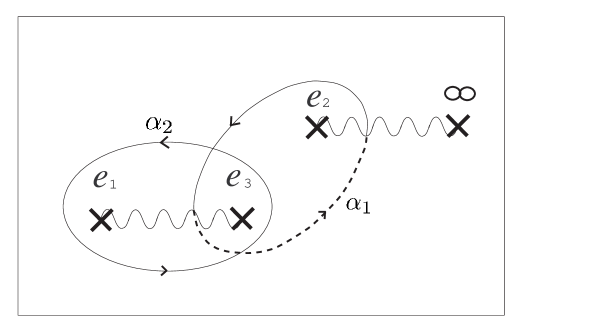
FIG. 1.: The contours $\alpha_{1}$ and $\alpha_{2}$.

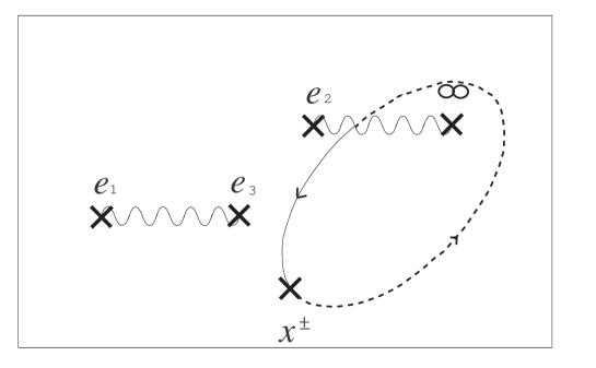
FIG. 2.: The contour of the integral Eq. (92).

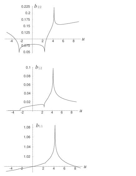
FIG. 3.: The effective gauge couplings $b_{ij}$ for $a_{1}=\sqrt{2}$ along real $u$-axis.

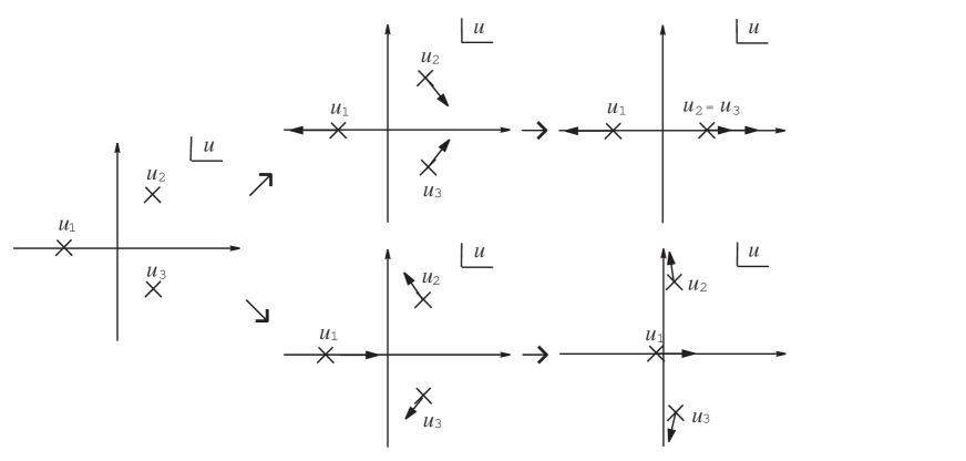
FIG. 4.: The flow of the singular points on $u$-plane for fixed $a_{1}$ in the case Im$a_{1}=0$. The left figure shows the positions of the singular points for $a_{1}=0$, the upper figures shows the evolutions of the singular points for $a_{1}>0$, and the lower figures show them as $a_{1}<0$ is decreasing.

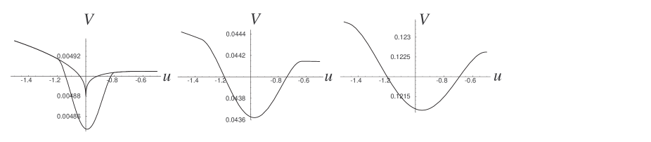
FIG. 5.: The effective potential around the $(2,1)_{1}$ dyon point for $a_{1}=0$ and $\xi=0.1$, $0.3$, $0.5$ (from left to right) along real $u$-axis.

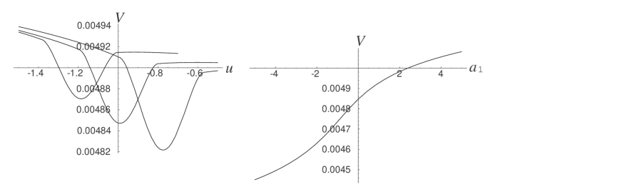
FIG. 6.: The left figure shows the effective potential for $a_{1}=1/8$ (left), $0$ (middle), $-1/8$ (right). The right figure shows the evolution of the potential energy along the flow of the $(2,1)_{1}$ dyon point.

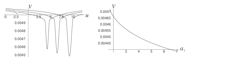
FIG. 7.: The left figure shows the effective potential along real $u$-axis for $a_{1}=\frac{2}{\sqrt{2}}$ (left), $\frac{2.5}{\sqrt{2}}$ (middle) and $\frac{3}{\sqrt{2}}$ (right). The right figure shows the evolution of the potential energy along the flow of the quark singular point.

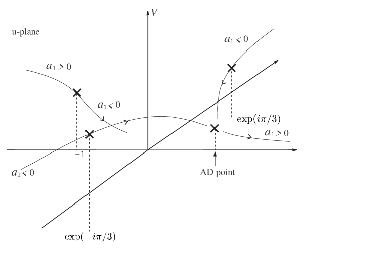
FIG. 8.: The evolutions of the potential energies along the flows of the singular points.

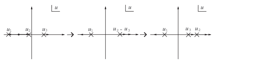
FIG. 9.: The flow of the singular points in the case Im$a_{1}=0$. The figures show the position of the singular points for $a_{1}=0$, $a_{1}=\frac{\Lambda_{2}}{2\sqrt{2}}$ and $a_{1}>\frac{\Lambda_{2}}{2\sqrt{2}}$ from left to right.

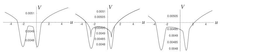
FIG. 10.: The effective potential for $a_{1}=0.3$ (left), $a_{1}=0.4$ (middle) and $a_{1}=0.5$ (right).

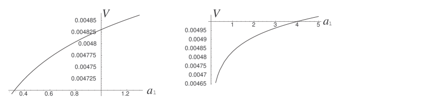
FIG. 11.: The evolutions of the potential energies along the flows of the $(1,1)_{-1}$ dyon point (left) and the $(1,1)_{1}$ dyon point (right).

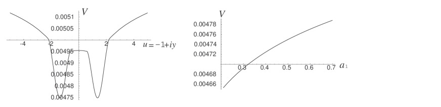
FIG. 12.: The effective potential (left) for $a_{1}=i\frac{\sqrt{2}}{4}$ along imaginary $u$-axis with Re$u=-1$, and the evolution of the potential energy (right) along the flow of the singular point $u_{1}$ in the case Re$a_{1}=0$.

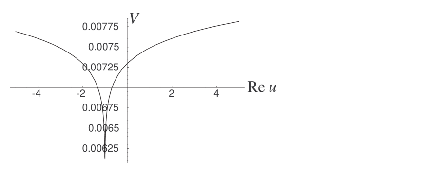
FIG. 13.: The effective potential without the contribution of the dyon condensations in the limit $a_{1}\rightarrow 0$.

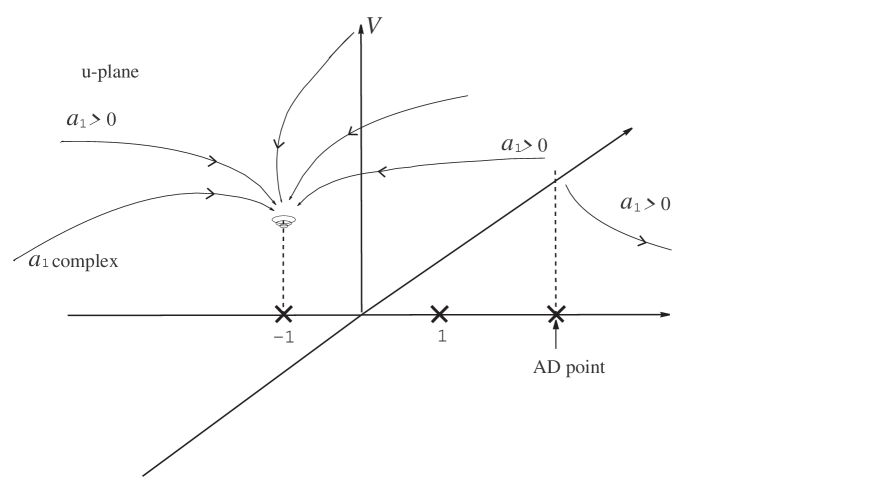
FIG. 14.: The evolutions of the potential energies along the flows of the singular points.

REFERENCES

- [1] N. Seiberg, Phys. Lett. B 318, 469 (1993); N. Seiberg, Phys. Rev. D 49, 6857 (1994); K. Intriligator, R.G. Leigh and N. Seiberg, Phys .Rev. D 50, 1092 (1994).
- [2] N. Seiberg and E. Witten, Nucl. Phys. B 426, 19 (1994).
- [3] N. Seiberg and E. Witten, Nucl. Phys. B 431, 484 (1994).
- [4] O. Aharony, J. Sonnenshein, M.E. Peskin and S. Yankielowicz, Phys. Rev. D 52, 6157 (1995).
- [5] N. Evans, S.D.H. Hsu and M. Schwetz, Phys. Lett. B 355, 475 (1995); N. Evans, S.D.H. Hsu and M. Schwetz, Nucl. Phys. B 456, 205 (1995).
- [6] L. Alvarez-Gaume, J. Distler, C. Kounnas and M. Marino, Int. J. Mod. Phys. A 11, 4745 (1996).
- [7] L. Alvarez-Gaume and M. Marino, Int. J. Mod. Phys. A 12, 975 (1997).
- [8] L. Alvarez-Gaume, M. Marino and F. Zamora, Int. J. Mod. Phys. A 13, 403 (1998); ibid 13, 1847 (1998).
- [9] N. Arkani-Hamed and R. Rattazzi, Phys.Lett. B 454, 290 (1999); M.A. Luty and R. Rattazzi, JHEP 11, 001 (1999).
- [10] P. Fayet, Nucl. Phys. B 113, 135 (1976).
- [11] M. Arai and N. Kitazawa, Proceeding of JINR Workshop “Supersymmetry and Quantum symmetry” (2000) 169; hep-th/9904214.
- [12] V.A. Miransky, Phys. Lett. 91B, 421 (1980); P.I. Fomin, V.P. Gusynin, V.A. Miransky and Yu. A. Sitenko, Riv. Nuov. Cim. 6, 1 (1983); V.A. Miransky, Nuov. Cim. 90A, 149 (1985).
- [13] A. Klemm, W. Lerche, S. Theisen and S. Yankielowicz, Int. J. Mod. Phys. A 11, 1929 (1996).
- [14] K. Ito and S.-K. Yang, Phys. Lett. B 366, 165 (1996).
- [15] A. Bilal and F. Ferrari, Nucl. Phys. B 480, 589 (1996).
- [16] J. M. Isidro, A. Mukherjee, J. P. Nunes and H. J. Schnitzer, Nucl. Phys. B 492, 647 (1997).
- [17] T. Masuda and H. Suzuki, Int. J. Mod. Phys. A 12, 3413 (1997).
- [18] A. Brandhuber and S. Stieberger, Int. J. Mod. Phys. A13, 1329 (1998).
- [19] A. Bilal and F. Ferrari, Nucl. Phys. B 516, 175 (1998).
- [20] A. Erdelyi et al., Higher Transcendental Functions, Vol. 1, McGraw-Hill, New york (1953).
- [21] P. Griffiths and J. Harris, Principles of Algebraic geometry, New York, John Wiley (1978).
- [22] P. C. Argyres and M. R. Douglas, Nucl. Phys. B 448, 93 (1995); P.C. Argyres, R. Plesser, N. Seiberg and E. Witten, Nucl. Phys. B 461, 71 (1996).