YITP-01-20

hep-th/0103146

March 2001

Torus-like Dielectric D2-brane

Yoshifumi Hyakutake

Yukawa Institute for Theoretical Physics, Kyoto University

Sakyo-ku, Kyoto 606-8502, Japan

ABSTRACT

We find new solutions corresponding to torus-like generalization of dielectric D2-brane from the viewpoint of D2-brane action and $N$ D0-branes one. These are meta-stable and would decay to the spherical dielectric D2-brane.

1 Introduction and Preliminaries

Type II superstring theories possess stringy solitons called Dirichlet-branes (D-branes) and they have been attracting our attention as a clue to resolve the non-perturbative aspects. As originally defined, a D$p$-brane is a $(p\!+\!1)$-dimensional hypersurface in 10-dimensional space-time on which open strings are allowed to end and the massless modes of the open strings form a multiplet of supersymmetric $U(1)$ gauge theory, a vector field $A_{a}$, $(9\!-\!p)$ real scalar fields $\Phi^{i}$ and their superpartners[1]. We will use $a,b$ for world-volume indices of D$p$-branes, $i,j,k$ for transverse indices of that and $\mu,\nu$ for space-time indices.

The bosonic part of the low energy theory on a single D$p$-brane world-volume is described by an abelian Born-Infeld action of the form[2]

$$\mathcal{S}_{\text{BI}} =-T_{p}\!\int\!\!d\!\stackrel{{\scriptstyle p+1}}{{\!\!\!\sigma}}\!e^{-\phi}\sqrt{-\det(P[G_{ab}+B_{ab}]+\lambda F_{ab})}\;,$$ (1)

where $T_{p}=2\pi/(2\pi\ell_{s})^{p+1}g_{s}$ is the D$p$-brane tension and $\lambda=2\pi\ell_{s}^{2}$. $F_{ab}$ is a field strength of the gauge field on the world-volume theory. A dilaton $\phi$, a metric $G_{\mu\nu}$ and an antisymmetric tensor $B_{\mu\nu}$, which are generically called Neveu-Schwartz fields, are fields in the space-time, so they appear in the above action as pullbacks to the world-volume. We’ll use the symbol $P[\cdots]$ to clarify the pullbacks, for example, $P[G_{ab}]=\frac{\partial x^{\mu}}{\partial\sigma^{a}}\frac{\partial x^{\nu}}{\partial\sigma^{b}}G_{\mu\nu}$. To simplify the action we often employ the static gauge

$$\begin{cases}x^{a}=\sigma^{a},\quad&a=0,1,\cdots,p\;,\\ x^{i}=\lambda\Phi^{i}(x^{a}),\quad&i=p\!+\!1,\cdots,9\;.\end{cases}$$ (2)

In this case $P[G_{ab}]$ is written as

$$P[G_{ab}] =G_{ab}+\lambda(\partial_{a}\Phi^{i}G_{ib}+\partial_{b}\Phi^{i}G_{ai})+\lambda^{2}\partial_{a}\Phi^{i}\partial_{b}\Phi^{j}G_{ij}.$$ (3)

One of the important features of the abelian Born-Infeld action is that it can capture some geometrical informations about the D$p$-brane and strings attached to or dissolved in it[3, 4, 5, 6, 7]. For instance, in the case of a D3-brane world-volume theory, a point charge Coulomb gauge field become a BPS saturated solution if one of the scalar fields, say $\Phi^{9}$, is exited. The excitation of $\Phi^{9}$ implies that the shape of the D3-brane is like a spike and, indeed, this configuration is identified with a fundamental string attached to the D3-brane[3].

In addition to the massless NS spectrums, closed strings in type II superstring theories contain Ramond-Ramond massless spectra. A D-brane carries an R-R charge and couples to R-R potentials as[8, 9, 10]

$$\mathcal{S}_{\text{CS}}=\mu_{p}\!\int_{p+1}P\big{[}\sum_{n\leq p\!+\!1}C^{(n)}e^{B}\big{]}e^{\lambda F}.$$ (4)

This is an abelian Chern-Simons action for the single D$p$-brane. Here $\mu_{p}=T_{p}$ is the R-R charge of the D$p$-brane and $C^{(n)}$ denotes the R-R $n$-form potential. $n$ takes odd $(1,3,5,7,9)$ for type IIA and even $(0,2,4,6,8,10)$ for type IIB. In the presence of non-zero R-R field strength $G^{(n+1)}=dC^{(n)}$, the abelian Chern-Siomons action gives some contribution to potential energy of the D$p$-brane world-volume theory, which implies existences of new solutions. For example, a spherical D2-brane, in the $x^{1},x^{2},x^{3}$ directions, with $N$ magnetic fluxes is usually unstable against decaying to $N$ D0-branes. In the background of constant $G^{(4)}_{0123}=-4h$, however, this spherical D2-brane expanding in the $x^{1},x^{2},x^{3}$ directions with a radius $h\lambda N$ becomes globally stable. This is so-called a dielectric effect or spherically dielectric D2-brane[11].

Low energy world-volume action for the single D$p$-brane is realized by the abelian Born-Infeld action $(\ref{eq:BI})$ plus the abelian Chern-Simons action $(\ref{eq:Che})$. Now we move on to a world-volume action for $N$ coincident D$p$-branes. If $N$ parallel D$p$-branes close to each other, the ground state modes of open strings stretched between these D$p$-branes become massless and therefore world-volume gauge symmetry is enhanced to $U(N)$[13]. To obtain the world-volume action of the $N$ coincident D$p$-branes, in the actions $(\ref{eq:BI})$ and $(\ref{eq:Che})$, we would modify $A_{a}$ and $\Phi^{i}$ as adjoint representations of $U(N)$ Lie algebra and take a trace of the integrand. The action obtained like this way, however, is not consistent with T-duality. The correct one is given by Myers et al. as follows[11, 12, 14, 15].

The non-abelian Born-Infeld action for the $N$ coincident D$p$-branes, which is consistent with T-duality, is modified into the form

$$\mathcal{S}_{\text{BI}} =-T_{p} \!\!\int\!\!d\!\stackrel{{\scriptstyle p+1}}{{\!\!\!\sigma}}\!\text{STr}\bigg{(}\!\!e^{-\phi}\!\!\sqrt{\!-\det\big{(}P[E_{ab}]\!+\!P[E_{ai}({(Q^{-1})^{i}}_{j}\!-\!{\delta^{i}}_{j})E^{jk}E_{kb}]\!+\!\lambda F_{ab}\big{)}\det\big{(}{Q^{i}}_{j}\big{)}}\bigg{)},$$ (5)

where $E_{\mu\nu}\!=\!G_{\mu\nu}\!+\!B_{\mu\nu}$ and ${Q^{i}}_{j}\!=\!{\delta^{i}}_{j}\!+\!i\lambda[\Phi^{i},\Phi^{k}]E_{kj}$. The partial derivatives $\partial_{a}\Phi^{i}$ are changed to covariant derivatives $D_{a}\Phi^{i}\!\equiv\!\partial_{a}\Phi^{i}\!+\!i[A_{a},\Phi^{i}]$. STr represents a symmetrized trace, that is, $U(N)$ Lie algebra indices of $F_{ab}$, $D_{a}\Phi^{i}$ and $i[\Phi^{i},\Phi^{j}]$ are symmetrized in the trace. By setting $\phi=B_{\mu\nu}=0$ and expanding around $G_{\mu\nu}=\eta_{\mu\nu}$, the non-abelian Born-Infeld action is approximated of the form

$$\mathcal{S}_{\text{BI}} \sim-NT_{p}V_{p+1}-\frac{\lambda^{2}}{4}T_{p}\!\!\int\!\!d\!\stackrel{{\scriptstyle p+1}}{{\!\!\!x}}\!\text{Tr}\Big{(}F^{ab}F_{ab}+2(D^{a}\Phi^{i})(D_{a}\Phi^{i})-[\Phi^{i},\Phi^{j}][\Phi^{i},\Phi^{j}]\Big{)}.$$ (6)

This action is also obtained by the dimensional reduction of the bosonic part of 10-dimensional $U(N)$ SYM theory to $(p+1)$-dimensional theory. It is easy to see that the potential term $-[\Phi^{i},\Phi^{j}]^{2}$ is characteristic of the non-abelian case, which originally comes from the term $\sqrt{\det Q}$. This potential term reaches to global minima when all $\Phi^{i}$ are simultaneously diagonalized. The diagonal elements of each $\Phi^{i}$ multiplied by $\lambda$ represent the positions of the individual D$p$-branes in the $x^{i}$ direction.

The non-abelian Chern-Simons action for the $N$ coincident D$p$-branes , which is consistent with T-duality, is modified into the form

$$\mathcal{S}_{\text{CS}} =\mu_{p}\!\int_{p+1}\text{STr}\Big{(}P\big{[}e^{i\lambda{\rm i}_{\Phi}{\rm i}_{\Phi}}\big{(}\sum_{n}C^{(n)}e^{B}\big{)}\big{]}e^{\lambda F}\Big{)},$$ (7)

where $n$ takes odd for type IIA and even for type IIB. Here $\rm{i}_{\Phi}$ denotes the interior product defined as

$$({\rm i}_{\Phi}{\rm i}_{\Phi})^{l}C^{(n+2l)}=\frac{1}{2^{l}n!}\Big{(}\prod_{s=1}^{l}[\Phi^{j_{2s}},\Phi^{j_{2s-1}}]\Big{)}C^{(n+2l)}_{j_{1}j_{2}\cdots j_{2l-1}j_{2l}\mu_{1}\cdots\mu_{n}}dx^{\mu_{1}}\wedge\cdots\wedge dx^{\mu_{n}}.$$ (8)

The remarkable property of the non-abelian Chern-Simons action is that there are coupling terms to the R-R potential $C^{(n)}$ with $n\geq p+3$. Because of this fact, a non-zero constant R-R field strength $G^{(p+4)}$ generates a new potential term for the $N$ coincident D$p$-branes world-volume theory. For instance, in the presence of the constant $G^{(4)}_{0123}=-4h$, the configurations of $N$ static D0-branes, i.e. all simultaneously diagonalized $\Phi^{i}$, are no longer globally stable. The potential energy reaches to global minima when $\frac{\Phi^{1}}{2h}$, $\frac{\Phi^{2}}{2h}$ and $\frac{\Phi^{3}}{2h}$ satisfy the commutation relation of the $SU(2)$ Lie algebra. These solutions are known as fuzzy two-spheres. If $\frac{\Phi^{1}}{2h}$, $\frac{\Phi^{2}}{2h}$ and $\frac{\Phi^{3}}{2h}$ belong to the $N$ dimensional irreducible representations of $SU(2)$ Lie algebra, the radius of the fuzzy two-sphere is almost equal to $h\lambda N$. This is the dielectric effect viewed from the $N$ D0-branes world-volume theory, often called Myers effect.

In this paper we explore torus-like configurations of the dielectric D2-brane from the two alternative viewpoint of the single D2-brane action or the $N$ D0-branes one. Motivations are as follows. Firstly, consider a situation where the spherical D2-brane (the fuzzy two-sphere) is expanding in the $x^{1},x^{2},x^{3}$ directions and the $x^{3}$ direction is compactified on a circle with circumference $2\ell$. The radius of the spherical D2-brane (the fuzzy two-sphere) is given by $h\lambda N$ in the background of constant $G^{(4)}_{0123}=-4h$ flux. Therefore, if $h\lambda N$ is bigger than $\ell$, the spherical D2-brane (the fuzzy two-sphere) would be deformed to a torus-like configuration via tachyon condensation process. Notice that one of two cycles of this torus wraps the $x^{3}$ direction but another does not wind any circle of the target space. It might difficult to pursuit the tachyon condensation process directly. However, knowledges of possible torus-like configurations of the dielectric D2-brane (the $N$ D0-branes) would tell us what happens after the tachyon condensation. The another reason is that the torus-like dielectric D2-brane ($N$ D0-branes) would be possible to regard as a non-BPS D-string which wraps the $x^{3}$ direction. A non-BPS D-string can be constructed from the D2-$\overline{\text{D}2}$ system by the condensation of a real tachyonic field. To make it more clear, consider the case where D2 and $\overline{\text{D}2}$ are extending in the $x^{2},x^{3}$ directions and separated by the string scale in the $x^{1}$ direction. If the tachyon condensation starts from $x^{2}=\pm\infty$ and proceed step by step toward $x^{2}=0$, a torus-like D2-brane can be obtained. A non-BPS D-string is identified to this torus-like D2-brane if the cycle, which doesn’t wind any circle of the target space, shrinks almost to zero. The constant R-R flux, however, might puff up this shrinking cycle. It is interesting if we can construct a non-BPS D-string via $N$ D0-branes.

In section 2 we review the dielectric effect briefly. In section 3 the torus-like configurations of the dielectric D2-brane are obtained as classical solutions of equation of motion for the D2-brane world-volume action. We try to reproduce the same configurations from the viewpoint of the $N$ D0-branes action in section 4. In section 5 we make some discussions.

2 Brief Review of the Dielectric Effect

The world-volume theory of $N$ coincident D$p$-branes is described by non-abelian Born-Infeld action plus non-abelian Chern-Simons action, which are consistent with T-duality[11, 12, 14, 15]. The remarkable fact is that, in the presence of constant R-R 4-form field strength, the $N$ coincident D0-branes are unstable against expanding into a spherical D2-brane[11]. In this section we briefly review this dielectric effect.

2.1 The Dielectric Effect from the D2-brane Action

In this subsection we shortly see the dielectric effect from the viewpoint of a single D2-brane world-volume theory. The system considered here is the spherical D2-brane with $N$ magnetic fluxes in the presence of constant R-R flux $G^{(4)}_{0123}=-4h$. The space-time flat metric is taken to be

$$ds^{2}=-dt^{2}+dr^{2}+r^{2}d\theta^{2}+r^{2}\sin^{2}\theta\,d\phi^{2}+\sum_{s=4}^{9}(dx^{s})^{2}.$$ (9)

Here the $x^{1}$, $x^{2}$ and $x^{3}$ directions are expressed by the spherical coordinates as

$$x^{1}=r\sin\theta\cos\phi,\quad x^{2}=r\sin\theta\sin\phi,\quad x^{3}=r\cos\theta.$$ (10)

Instead of the usual static gauge, it is useful to take the world-volume coordinates of the spherical D2-brane as $\sigma^{0}\!=\!t$, $\sigma^{1}\!=\!\theta$, $\sigma^{2}\!=\!\phi$. Suppose that the position of the spherical D2-brane is at $r\!=\!R$ and $x^{s}\!=\!0$. The R-R flux on the spherical coordinates is $G^{(4)}_{tr\theta\phi}=-4hr^{2}\sin\theta$, or $C^{(3)}_{t\theta\phi}=\frac{4}{3}hr^{3}\sin\theta$ in terms of the R-R potential. The field strength of the gauge field is given by $F_{\theta\phi}=\frac{1}{2}N\sin\theta$ and other fields are set to be zero.

In these backgrounds, the world-volume action of the spherical D2-brane is given by

$${\mathcal{S}}_{\text{D2}} =-T_{2}\int\!\!dtd\theta d\phi\sqrt{-\det(P[G_{ab}]+\lambda F_{ab})}+\mu_{2}\int P[C^{(3)}]$$

$$=-4\pi T_{2}\int\!\!dt\bigg{(}\sqrt{R^{4}+\frac{\lambda^{2}N^{2}}{4}}-\frac{4h}{3}R^{3}\bigg{)}.$$ (11)

Thus, the potential energy is expressed by a function of $R$ as

$$V_{\text{D2}}(R)=\sqrt{\big{(}4\pi R^{2}T_{2}\big{)}^{2}+\big{(}NT_{0}\big{)}^{2}}-\frac{16\pi}{3}hT_{2}R^{3}.$$ (12)

The first term is just the square root of the sum of the spherical D2-brane mass squared and $N$ D0-branes mass squared. If we assume $4\pi R^{2}T_{2}\ll NT_{0}$, this potential energy can be approximated as

$$V_{\text{D2}}(R) \sim NT_{0}+\frac{2T_{0}}{\lambda^{2}N}R^{4}-\frac{8hT_{0}}{3\lambda}R^{3}.$$ (13)

This approximated potential energy takes extrema at $R\!=\!0,h\lambda N$. The potential energies at these points are $V_{\text{D2}}(0)\!=\!NT_{0}$ and $V_{\text{D2}}(h\lambda N)\!=\!NT_{0}-\frac{2}{3}NT_{0}(h^{2}\lambda N)^{2}$ respectively, so the spherical D2-brane with $R\!=\!h\lambda N$ is stable. In this case the above assumption insists $h^{2}\lambda N\ll 1$.

Before proceeding to the next subsection we should estimate a region where our calculations so far are reliable. If we take a typical length of the system to be $R_{\text{sys}}$, dimensionless square of gauge coupling constant on the D2-brane is given by $g_{\text{gauge}}^{2}R_{\text{sys}}\sim g_{s}R_{\text{sys}}/\ell_{s}$ and that of gravitational coupling constant becomes $\kappa^{2}/R_{\text{sys}}^{8}\sim\ell_{s}^{8}g_{s}^{2}/R_{\text{sys}}^{8}$. The Born-Infeld action is valid where $g_{\text{gauge}}^{2}R_{\text{sys}}$ is fixed and the gravitational interactions are neglected, i.e., in the decoupling limit $\ell_{s}\ll R_{\text{sys}}$ and $g_{s}\ll 1$. So in the case of $R\!=\!h\lambda N$, we should require $\ell_{s}\ll h\lambda N$.

2.2 Myers Effect

In this subsection we study the dielectric effect from the viewpoint of $N$ coincident D0-branes. The world-volume action employed here is (6) plus (7). The $\Phi^{4},\cdots,\Phi^{9}$ are set to be zero. Now the world-volume action of the $N$ coincident D0-branes in the background of constant R-R flux $G^{(4)}_{0123}=-4h$ is given by

$${\mathcal{S}}_{\text{$N$D0}} \sim-\!NT_{0}V_{1}\!+\!\frac{\lambda^{2}}{4}T_{0}\!\!\int\!\!dt\,\text{Tr}\Big{(}2(\partial_{t}\Phi^{i})^{2}\!+\![\Phi^{i},\Phi^{j}][\Phi^{i},\Phi^{j}]\Big{)}\!-\!\frac{2ih\lambda^{2}}{3}\mu_{0}\,\epsilon_{ijk}\!\!\int\!\!dt\,\text{Tr}\Big{(}\Phi^{i}[\Phi^{j},\Phi^{k}]\Big{)},$$ (14)

where $i,j,k$ run $1,2,3$. This action is valid when the commutators $i\lambda[\Phi^{i},\Phi^{j}]$ are small enough. The potential energy can be written as

$$V_{\text{$N$D0}}=NT_{0}-\frac{\lambda^{2}}{4}T_{0}\text{Tr}\Big{(}[\Phi^{i},\Phi^{j}][\Phi^{i},\Phi^{j}]\Big{)}+\frac{2ih\lambda^{2}}{3}\mu_{0}\,\epsilon_{ijk}\text{Tr}\Big{(}\Phi^{i}[\Phi^{j},\Phi^{k}]\Big{)}.$$ (15)

And in the static case, the equation of motion is obtained by varing the potential energy,

$$\frac{\delta V_{\text{$N$D0}}}{\delta\Phi^{i}}=\lambda^{2}T_{0}\,[[\Phi^{i},\Phi^{j}],\Phi^{j}]+2ih\lambda^{2}\mu_{0}\,\epsilon_{ijk}[\Phi^{j},\Phi^{k}]=0.$$ (16)

All simultaneously diagonalized $\Phi^{i}$ are one of the solutions of this equation of motion, where the potential energy is equal to $NT_{0}$. On the other hand, we can find more nontrivial solutions which satisfy the relation of $SU(2)$ Lie algebra

$$\Big{[}\frac{\Phi^{i}}{2h},\frac{\Phi^{j}}{2h}\Big{]} =i\epsilon_{ijk}\frac{\Phi^{k}}{2h}.$$ (17)

The non-commutative geometry which satisfies the above relation is often called fuzzy two-sphere. If all $\Phi^{i}/2h$ belong to $N$ dimensional irreducible representations of $SU(2)$ Lie algebra, the radius of the fuzzy two-sphere is given by

$$R_{\text{fuzzy}}\equiv\sqrt{\frac{1}{N}\text{Tr}\big{(}(\lambda\Phi^{i})^{2}\big{)}}=h\lambda N\sqrt{1-\frac{1}{N^{2}}}\;,$$ (18)

and the potential energy can be estimated as

$$V_{\text{$N$D0}} =NT_{0}-\frac{2}{3}NT_{0}(h^{2}\lambda N)^{2}\Big{(}1-\frac{1}{N^{2}}\Big{)}.$$ (19)

This potential energy is less than that of the all simultaneously diagonalized solutions and this means that the fuzzy two-sphere is stable. If the $N$ is large, the radius and the potential energy of the fuzzy two-sphere match up to those of the spherical D2-brane calculated in the previous subsection up to $1/N^{2}$ correction.

As a preparation for a later section, we examine the geometry of the fuzzy two-sphere in detail. By using variables

$$J_{+}=\frac{\Phi^{1}}{2h}+i\frac{\Phi^{2}}{2h}\;,\quad J_{-}=\frac{\Phi^{1}}{2h}-i\frac{\Phi^{2}}{2h}\;,\quad J_{3}=\frac{\Phi^{3}}{2h}\;,$$ (20)

the equation of motion (16) is rewritten as

$$\big{[}[J_{+},J_{-}],J_{+}\big{]}+2\big{[}[J_{+},J_{3}],J_{3}\big{]}+4[J_{+},J_{3}]=0\;,$$ (21)

$$\big{[}[J_{+},J_{3}],J_{-}\big{]}+\big{[}[J_{-},J_{3}],J_{+}\big{]}+2[J_{+},J_{-}]=0\;.$$

In the case of the fuzzy two-sphere, $J_{+}$ and $J_{-}$ are ladder operators of $SU(2)$ Lie algebra and $J_{3}$ is the Cartan subalgebra. The explicit matrix form of $J_{3}$ in the $N$ dimensional irreducible representation is given by

$$J_{3}^{\text{irr}}=\begin{pmatrix}\;\frac{N-1}{2}&&&&\;\\ \>&\frac{N-3}{2}&&&\;\\ \;&&\ddots&&\;\\ \;&&&-\frac{N-3}{2}&\;\\ \;&&&&-\frac{N-1}{2}\;\end{pmatrix},$$ (22)

where the superscript is to denote the irreducibility. Each diagonal element multiplied by $2h\lambda$ would be interpreted as the position of each D0-brane in the $x^{3}$ direction. Here we call the D0-brane corresponding to the $(m,m)$ element as the $m$th D0-brane. The explicit matrix forms of $J_{+}$ and $J_{-}$ belonging to the $N$ dimensional irreducible representations are given by

$$J_{+}^{\text{irr}}=\begin{pmatrix}\;0&\sqrt{N\!\!-\!\!1}&&&\;\\ \>&0&\!\!\!\!\!\!\sqrt{2(N\!\!-\!\!2)}\!\!\!\!&&\;\\ \;&&\ddots&&\;\\ \;&&&0&\sqrt{N\!\!-\!\!1}\;\\ \;&&&&0\;\end{pmatrix}\;,\;J_{-}^{\text{irr}}=\begin{pmatrix}\;0&&&&\;\\ \>\sqrt{N\!\!-\!\!1}&0&&&\;\\ \;&\!\!\!\!\!\!\sqrt{2(N\!\!-\!\!2)}\!\!&\ddots&&\;\\ \;&&&0&\;\\ \;&&&\!\!\sqrt{N\!\!-\!\!1}&0\;\end{pmatrix}.$$ (23)

The off-diagonal elements $(m,m\!+\!1)$ or $(m\!+\!1,m)$ multiplied by $2h\lambda$ would represent the extension, to the radial direction of the $x^{1}$-$x^{2}$ plane, of the cell between the $m$th D0-brane and the $(m\!+\!1)$th D0-brane. The factor $2h\lambda$ is defined by the fact that $\text{Tr}\big{(}(\lambda\Phi^{1})^{2}\big{)}+\text{Tr}\big{(}(\lambda\Phi^{2})^{2}\big{)}$ is equal to $(2h\lambda)^{2}\text{Tr}\big{(}J_{+}J_{-}\big{)}$.

On the arguments so far, we chose the irreducible representations of $SU(2)$ Lie algebra as the solution of (21). But reducible representations of $SU(2)$ can also be the solutions. For example $2N\!\times\!2N$ matrices,

$$J_{3}=\begin{pmatrix}J_{3}^{\text{irr}}\!+\!c\mathbf{1}_{N\times N}&0\\ 0&J_{3}^{\text{irr}}\!-\!c\mathbf{1}_{N\times N}\end{pmatrix},\quad J_{+}=\begin{pmatrix}J_{+}^{\text{irr}}&0\\ 0&J_{+}^{\text{irr}}\end{pmatrix},\quad J_{-}=\begin{pmatrix}J_{-}^{\text{irr}}&0\\ 0&J_{-}^{\text{irr}}\end{pmatrix},$$ (24)

become a solution and represent two fuzzy two-spheres located at $x^{3}=2h\lambda c$ and $x^{3}=-2h\lambda c$ respectively. The potential energy of this solution is higher than that of a fuzzy two-sphere which is constructed by $2N$ dimensional irreducible representations, but lower than that of $N$ coincident D0-branes.

Since each component of the commutators $i\lambda[\Phi^{i},\Phi^{j}]$ is of the order of $h^{2}\lambda N$, our calculations are reliable when a relation $h^{2}\lambda N\ll 1$ holds.

3 A Torus-like Dielectric D2-brane

In this section we find out configurations of a torus-like D2-brane with $N$ magnetic fluxes in the presence of constant R-R flux $G^{(4)}_{0123}=-4h$. The $x^{3}$ direction is compactified by a circle with the circumference $2\ell$. One of two cycles of the torus-like D2-brane wraps the $x^{3}$ direction, but another doesn’t wind any circle of the target space. This will be an extension of the spherical D2-brane solution.

Let us consider a case where the center of the spherical dielectric D2-branes is located at $x^{3}=0$ (Fig.1 (a)). Since the radius of the spherical D2-brane is given by $h\lambda N$, adjacent surfaces of the spherical D2-brane approach at the length of a string scale at $h\lambda N\sim\ell$. There arise a tachyonic mode in the spectrum of the open strings stretched between those surfaces (Fig.1 (b)). This tachyonic mode would imply a deformation of the topology of the sphere and, at $h\lambda N>\ell$, the shape of the D2-brane will become a distorted torus (Fig.1 (c)). We call this configuration a torus-like dielectric D2-brane.

Figure 1: Configurations of the dielectric D2-brane. The $x^{3}$ direction is compactified with the circumference $2\ell$. (a) $h\lambda N\!<\!\ell$. (b) $h\lambda N\!\sim\!\ell$. (c) $h\lambda N\!>\!\ell$.

The world-volume theory on the D2-brane can be described by the abelian Born-Infeld action (1) plus the abelian Chern-Simons action (4). We consider the torus-like D2-brane with $N$ magnetic fluxes in the presence of the constant R-R 4-form filed strength $G^{(4)}_{0123}=-4h$, thus the relevant fields are the metric $G_{\mu\nu}$, the field strength of the gauge field $F_{ab}$ and the R-R 3-form potential $C^{(3)}$. Since the shape of the D2-brane is a distorted torus, instead of the static gauge, we employ the gauge

$$x^{0}=t,\quad x^{1}=R(t,z)\cos\theta,\quad x^{2}=R(t,z)\sin\theta,\quad x^{3}=z.$$ (25)

Here $(t,\theta,z)$ are the world-volume coordinates with $t\in\mathbb{R}$, $-\pi\leq\theta\leq\pi$, and $-\ell\leq z\leq\ell$.

Now the action of the D2-brane is written in the form

$${\mathcal{S}}_{\text{D2}} =-T_{2}\int\!\!dtd\theta dz\Big{(}\sqrt{-\det(P[G]_{ab}+\lambda F_{ab})}\Big{)}+\mu_{2}\int P[C^{(3)}]$$

$$=-T_{2}\int\!\!dtd\theta dz\bigg{\{}\sqrt{R^{2}(1+{R^{\prime}}^{2}-{\dot{R}}^{2})+(\lambda F_{\theta z})^{2}(1-{\dot{R}}^{2})}-2hR^{2}\bigg{\}},$$ (26)

where $\dot{R}$ and $R^{\prime}$ are abbreviations of $\frac{dR}{dt}$ and $\frac{dR}{dz}$ respectively. In order to obtain $F_{\theta z}$ as a functional of $R$, we use the equations of motion for $A_{\theta}$ and $A_{z}$. These equations lead that the quantity $D$ defined by

$$D\equiv-\frac{1}{\lambda T_{2}}\frac{\delta{\mathcal{L}}}{\delta F_{\theta z}}=\frac{\lambda F_{\theta z}(1-\dot{R}^{2})}{\sqrt{R^{2}(1+{R^{\prime}}^{2}-{\dot{R}}^{2})+(\lambda F_{\theta z})^{2}(1-{\dot{R}}^{2})}},$$ (27)

depends only on $t$. By using this $D$, $\lambda F_{\theta z}$ can be expressed as

$$\lambda F_{\theta z}=\frac{DR\sqrt{1+{R^{\prime}}^{2}-{\dot{R}}^{2}}}{\sqrt{(1-{\dot{R}}^{2})(1-{\dot{R}}^{2}-D^{2})}}.$$ (28)

We only consider the static case hereafter, $\dot{R}=0$ and $D$ is a constant. Then the eq.(28) becomes simply

$$\lambda F_{\theta z}=\frac{D}{\sqrt{(1-D^{2})}}R\sqrt{1+{R^{\prime}}^{2}}.$$ (29)

Since the metric on the world-volume is given by $ds^{2}=-dt^{2}+R^{2}d\theta^{2}+(1+{R^{\prime}}^{2})dz^{2}$, the eq.(29) means that the number of the magnetic fluxes per unit area is constant everywhere. Furthermore, $D$ can be determined by the quantization condition of the magnetic flux. Now the number of the magnetic fluxes on the D2-brane is $N$, the condition is written as

$$N=\frac{1}{2\pi}\int d\theta dzF_{\theta z}=\frac{1}{2\pi\lambda}\frac{D}{\sqrt{(1-D^{2})}}S.$$ (30)

Here $S$ is the area of the D2-brane world-volume,

$$S=\int d\theta dzR\sqrt{1+{R^{\prime}}^{2}}.$$ (31)

The field strength of the gauge field, therefore, becomes

$$\lambda F_{\theta z}=\frac{2\pi\lambda N}{S}R\sqrt{1+{R^{\prime}}^{2}}.$$ (32)

Using this expression, the action (26) is rewritten in the form

$${\mathcal{S}}_{\text{D2}}=-T_{2}\int\!\!dt\sqrt{S^{2}+\big{(}2\pi\lambda N\big{)}^{2}}+4\pi hT_{2}\int\!\!dtdzR^{2}.$$ (33)

and the potential energy is given by

$$V_{\text{D2}}=\sqrt{\big{(}ST_{2}\big{)}^{2}+\big{(}NT_{0}\big{)}^{2}}-4\pi hT_{2}\int\!\!dzR^{2}.$$ (34)

The first term is the square root of the sum of the D2-brane mass squared and $N$ D0-branes mass squared, as expected.

Now the potential energy is obtained as a functional of $R(z)$. The next task is to get the explicit form of $R(z)$. The equation of motion for $R$ is obtained by varing the potential energy.

$$\frac{\delta V_{\text{D2}}}{\delta R} =\frac{\partial V_{\text{D2}}}{\partial R}-\Big{(}\frac{\partial V_{\text{D2}}}{\partial R^{\prime}}\Big{)}^{\prime}$$

$$=\frac{\partial V_{\text{D2}}}{\partial S}\frac{\partial S}{\partial R}-8\pi hT_{2}R-\Big{(}\frac{\partial V_{\text{D2}}}{\partial S}\frac{\partial S}{\partial R^{\prime}}\Big{)}^{\prime}$$

$$=\frac{2\pi T_{2}}{R^{\prime}}\bigg{\{}\frac{R}{P\sqrt{1+{R^{\prime}}^{2}}}-2hR^{2}\bigg{\}}^{\prime}$$ (35)

$$=0.$$

Here $P$ is defined as

$$P=\sqrt{1+\Big{(}\frac{NT_{0}}{ST_{2}}\Big{)}^{2}}.$$ (36)

One can easily integrate the eq.(35) once and obtain

$$R^{\prime} =\pm\frac{2h}{2hR^{2}\!+\!C}\sqrt{(R_{+}^{2}-R^{2})(R^{2}-R_{-}^{2})},$$ (37)

where $C$ is an integration constant and $R_{\pm}^{2}$ are defined as

$$R_{\pm}^{2} \equiv\frac{C}{hX}\big{(}1-X/2\pm\sqrt{1-X}\big{)},$$ (38)

$$X \equiv 8ChP^{2}.$$

If $X\leq 1$, the eq.(37) shows that $R^{\prime}\!=\!0$ at $R\!=\!R_{\pm}$ and $R$ is periodic with $R_{-}\!\leq\!R\!\leq\!R_{+}$. Because we are studying the configurations like Fig.1(c), the minus (plus) sign of the eq.(37) is chosen in $0\!\leq\!z\!\leq\!\ell$ ($-\ell\!\leq\!z\!\leq\!0$). We only consider the region where $0\!\leq\!z\!\leq\!\ell$ in the following. The eq.(37) is further integrated as

$$z =\frac{1}{2h}\int_{R}^{R_{+}}\!\!\!\!dR\frac{2hR^{2}\!+\!C}{\sqrt{(R_{+}^{2}-R^{2})(R^{2}-R_{-}^{2})}}$$

$$=R_{+}\int_{0}^{\psi}\!\!d\phi\sqrt{1-k^{2}\sin^{2}\phi}+\frac{C}{2hR_{+}}\int_{0}^{\psi}\!\!d\phi\frac{1}{\sqrt{1-k^{2}\sin^{2}\phi}}$$ (39)

$$=R_{+}E(\psi,k)+\frac{C}{2hR_{+}}F(\psi,k),$$

where we choose such an integration constant that $R=R_{+}$ at $z=0$ and $R=R_{-}$ at $z=\ell$. $F(\psi,k)$ and $E(\psi,k)$ are the incomplete elliptic integrals of the first and second kinds respectively, $k$ is the elliptic modulus and $\psi$ is the angle given by

$$k =\frac{\sqrt{R_{+}^{2}-R_{-}^{2}}}{R_{+}},\quad\psi=\sin^{-1}\sqrt{\frac{R_{+}^{2}-R^{2}}{R_{+}^{2}-R_{-}^{2}}}.$$ (40)

The range of the elliptic modulus is $0\!\leq\!k\!\leq\!1$ and that of the angle is $0\!\leq\!\psi\!\leq\!\frac{\pi}{2}$. Some properties of the elliptic integrals are listed in the appendix A.

Now we will examine the solutions (39) in detail. For this purpose, it is better to express the quantities in terms of the modulus $k$. As we will see later, however, two distinct solutions correspond to the same $k$. In fact, $X\!=\!8ChP^{2}$ is more suitable for a parameter of solutions. By the definition (40), $k$ can be expressed as a function of $X$.

$$k^{2}=\frac{2\sqrt{1-X}}{1-X/2+\sqrt{1-X}}.$$ (41)

The range of $X$ is restricted to $X\!\leq\!1$, which is consistent with $0\!\leq\!k\!\leq\!1$. In general, two distinct values of $X$ correspond to the same $k$, for example, $k\!=\!0$ at $X\!=\!-\infty,1$. The only exception is $k\!=\!1$ at $X\!=\!0$. $k$ increase monotonously in the region of $X\!<\!0$, and decrease monotonously in that of $0\!<\!X\!<\!1$ (Fig.2).

Figure 2: $k$ as a function of $X$.

Now we rewrite the quantities obtained so far as functions of $X$. By the definition of $S$, we obtain

$$S=\frac{2\pi}{hP}\int_{R_{-}}^{R_{+}}\!\!\!\!dR\frac{R^{2}}{\sqrt{(R_{+}^{2}-R^{2})(R^{2}-R_{-}^{2})}}=\frac{2\pi R_{+}}{hP}E(k),$$ (42)

where $E(k)$ is the complete elliptic integral of the second kind. By using this equation (42), $P$ is written as

$$P=\frac{1}{\sqrt{1-\bigg{(}\dfrac{h\lambda N}{R_{+}E(k)}\bigg{)}^{2}}}.$$ (43)

By using this equation (43) and the definition of $X$ (38), we can rewrite the constant $C$ by means of $X$ as

$$C =\frac{X}{16h}\left(1-\sqrt{1-\frac{32(h^{2}\lambda N)^{2}}{E(k)^{2}\big{(}1\!-\!X/2\!+\!\sqrt{1\!-\!X}\big{)}}}\,\right)$$

$$\sim\frac{X(h^{2}\lambda N)^{2}}{hE(k)^{2}\big{(}1\!-\!X/2\!+\!\sqrt{1\!-\!X}\big{)}},$$ (44)

where $\sim$ holds when $h^{2}\lambda N\ll 1$. Here we take a choice which gives the smaller area. $S$ is now written in the form

$$S =4\pi(h\lambda N)^{2}\times\frac{2\sqrt{2}}{E(k)\sqrt{1\!-\!X/2\!+\!\sqrt{1\!-\!X}}}\left(1+\sqrt{1-\frac{32(h^{2}\lambda N)^{2}}{E(k)^{2}\big{(}1\!-\!X/2\!+\!\sqrt{1\!-\!X}\big{)}}}\,\right)^{-1}$$

$$\sim 4\pi(h\lambda N)^{2}\times\frac{\sqrt{2}}{E(k)\sqrt{1\!-\!X/2\!+\!\sqrt{1\!-\!X}}}.$$ (45)

In the limit of $h^{2}\lambda N\ll 1$, $S$ is equal to $4\pi(h\lambda N)^{2}$ at $X\!=\!0$. The solution of $X\!=\!0$, therefore, corresponds to the spherical D2-brane in the previous section.

$R_{\pm}$ are given by

$$R_{\pm}^{2} =\frac{1\!-\!X/2\!\pm\!\sqrt{1\!-\!X}}{16h^{2}}\left(1-\sqrt{1-\frac{32(h^{2}\lambda N)^{2}}{E(k)^{2}\big{(}1\!-\!X/2\!+\!\sqrt{1\!-\!X}\big{)}}}\,\right),$$

$$R_{+} \sim\frac{h\lambda N}{E(k)},$$ (46)

$$R_{-} \sim\frac{h\lambda N}{E(k)}\times\sqrt{\frac{1\!-\!X/2\!-\!\sqrt{1\!-\!X}}{1\!-\!X/2\!+\!\sqrt{1\!-\!X}}}.$$ (47)

$R_{+}\!=\!R_{-}$ when $X\!=\!1$, thus the shape of the D2-brane becomes a torus. Up to order $h^{2}\lambda N$, the radius of the cycle, which does not wind any circle of the target space, equals to $\frac{2}{\pi}h\lambda N$.

The half of the circumference of the $x^{3}$ circle $\ell$ is given by

$$\ell =R_{+}E(k)+\frac{C}{2hR_{+}}K(k)$$

$$=\frac{1}{4h}\!\!\left(E(k)\sqrt{1\!\!-\!\!X/2\!\!+\!\!\sqrt{1\!\!-\!\!X}}+\frac{K(k)X}{2\sqrt{1\!\!-\!\!X/2\!\!+\!\!\sqrt{1\!\!-\!\!X}}}\right)\!\!\sqrt{1\!-\!\sqrt{1\!-\!\frac{32(h^{2}\lambda N)^{2}}{E(k)^{2}\big{(}1\!\!-\!\!X/2\!\!+\!\!\sqrt{1\!\!-\!\!X}\big{)}}}\,}$$

$$\sim h\lambda N\times\left(1+\frac{K(k)X}{2E(k)\big{(}1\!\!-\!\!X/2\!\!+\!\!\sqrt{1\!\!-\!\!X}\big{)}}\right).$$ (48)

$K(k)$ is the complete elliptic integral of the first kind. Notice that $\ell$ depends on two quantities, $h\lambda N$ and $X$, in the limit of $h^{2}\lambda N\ll 1$. As it is usual to fix $\ell$, the eq.(48) is interpreted as a relation between $h\lambda N$ and $X$. $X$ and $h\lambda N$ govern the shape and size of the D2-brane respectively.

Finally $z$ is written as

$$z =\frac{1}{4h}\!\!\left(E(\psi,k)\sqrt{1\!\!-\!\!X/2\!\!+\!\!\sqrt{1\!\!-\!\!X}}+\frac{F(\psi,k)X}{2\sqrt{1\!\!-\!\!X/2\!\!+\!\!\sqrt{1\!\!-\!\!X}}}\right)\!\!\sqrt{1\!-\!\sqrt{1\!-\!\frac{32(h^{2}\lambda N)^{2}}{E(k)^{2}\big{(}1\!\!-\!\!X/2\!\!+\!\!\sqrt{1\!\!-\!\!X}\big{)}}}\,}$$

$$\sim h\lambda N\times\left(\frac{E(\psi,k)}{E(k)}+\frac{F(\psi,k)X}{2E(k)\big{(}1\!\!-\!\!X/2\!\!+\!\!\sqrt{1\!\!-\!\!X}\big{)}}\right),$$ (49)

and the potential energy is given by

$$V_{\text{D2}} =\sqrt{\big{(}ST_{2}\big{)}^{2}+\big{(}NT_{0}\big{)}^{2}}-4\pi hT_{2}\left\{\frac{4(2-k^{2})E(k)}{3}R_{+}^{3}-\frac{2(1-k^{2})K(k)}{3}R_{+}^{3}+E(k)\frac{CR_{+}}{h}\right\}$$

$$\sim NT_{0}-NT_{0}\left\{\frac{8(2-k^{2})}{3E(k)^{2}}-\frac{4(1-k^{2})K(k)}{3E(k)^{3}}-\frac{4-2X}{E(k)^{2}\big{(}1\!\!-\!\!X/2\!\!+\!\!\sqrt{1\!\!-\!\!X}\big{)}}\right\}(h^{2}\lambda N)^{2}.$$ (50)

The results in the limit of $h^{2}\lambda N\ll 1$ are collected in Table 1. As already mentioned, we see that $X\!=\!0$ corresponds to the spherical D2-brane which agrees with the one obtained in §§2.1 and $X\!=\!1$ corresponds to the toroidal D2-brane whose potential energy is equal to that of $N$ D0-branes. Even though the potential energy takes minimum for the spherical D2-brane, if $h^{2}\lambda N$ is small enough we could expect that the torus-like D2-branes are meta-stable.

The shapes of the torus-like D2-branes where $X\!=\!0$, $0.75$, $0.999$ $-3$, $-999$ are depicted in Fig.4. For these solutions, $R_{-}/h\lambda N=0$, $0.299$, $0.616$, $0.299$ ,$0.616$, respectively. The remarkable D2-brane configuration is like Fig.4(d). In this case, another torus-like D2-brane seems to appear in the interior of the original torus-like D2-brane(Fig.3). However, the world-volume of the D2-brane intersect at $z=\ell$. The space-metric would not be flat around there and our calculations might go wrong. For this reason, we do not take seriously the results for the region $-\infty<X<0$.

$X$	$-\infty$	$\cdots$	$0$ (sphere)	$\cdots$	$1$ (torus)
$\ell$	$0$	$\nearrow$	$h\lambda N$	$\nearrow$	$2h\lambda N$
$R_{+}$	$\frac{2}{\pi}h\lambda N$	$\nearrow$	$h\lambda N$	$\searrow$	$\frac{2}{\pi}h\lambda N$
$R_{-}$	$\frac{2}{\pi}h\lambda N$	$\searrow$	$0$	$\nearrow$	$\frac{2}{\pi}h\lambda N$
$V_{\text{D2}}$	$NT_{0}$	$\searrow$	$NT_{0}-\frac{2}{3}NT_{0}(h^{2}\lambda N)^{2}$	$\nearrow$	$NT_{0}$

Table 1: The behaviors of $\ell$, $R_{\pm}$ and $V_{\text{D2}}$ in the limit of $h^{2}\lambda N\ll 1$.

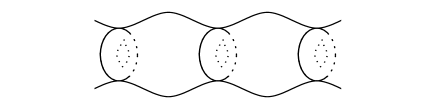
Figure 3: The case of $X<0$.

Figure 4: The shapes of D2-branes at $X\!\!=\!\!0$, $0.75$, $0.999$, $-3$ and $-999$. Vertical axes label $z/h\lambda N$ and horizontal axes label $R/h\lambda N$. $R_{-}/h\lambda N$ of (a), (b), (c), (d) and (e) are equal to $0$, $0.299$, $0.616$, $0.299$ and $0.616$ respectively.

4 Torus-like Generalization of Myers Effect

In the previous section, we obtained the various torus-like configurations of the D2-brane, including the spherical configuration. As we have seen in the §§2.2, the spherical dielectric D2-brane could also be obtained from the world-volume theory of the $N$ D0-branes. In this section, we express the torus-like D2-branes from the viewpoint of the world-volume theory of the $N$ D0-branes.

We consider the same system as in the §§2.2. The potential energy and the equation of motion are given by the eq.(15) and the eq.(21) respectively. Our aim is to find the torus-like solutions of the eq.(21). Let us start the explicit matrix forms of the spherical solution (22),(23). A small deformation of the spherical configuration would not change the positions of non-zero components in the matrices so much. Therefore, we assume the form of $J_{3}$ as

$$J_{3} =\begin{pmatrix}\;\ddots&&&&&&&&\;\\ \>&z_{N}\!\!+\!\!2\ell^{\prime}&&&&&&&\;\\ \;&&z_{1}&&&&&&\;\\ \;&&&z_{2}&&&&&\;\\ \>&&&&\ddots&&&&\;\\ \;&&&&&z_{N-1}&&&\;\\ \;&&&&&&z_{N}&&\;\\ \>&&&&&&&z_{1}\!\!-\!\!2\ell^{\prime}&\;\\ \;&&&&&&&&\ddots\;\end{pmatrix}.$$ (51)

Note that the compactification of the $x^{3}$ direction makes the size of matrix infinity. The $N\times N$ diagonal block containing the components $z_{1},\cdots,z_{N}$ are the original matrix and the others are the copies of it. $z_{1},\cdots,z_{N}$ multiplied by $2h\lambda$ denote the positions in the $x^{3}$ direction of $N$ D0-branes and $2\ell^{\prime}$ multiplied by $2h\lambda$ is the circumference of the compactified circle. We also assume the forms of $J_{\pm}$ as

$$J_{+}=J_{-}^{\dagger} =\begin{pmatrix}\;\ddots\!\!&R_{N\!-\!1}&&&&&&&\;\\ \>&0&R_{N}&&&&&&\;\\ \;&&0&\,\;R_{1}\;&&&&&\;\\ \;&&&0&&&&&\;\\ \>&&&&\;\ddots\;&&&&\;\\ \;&&&&&0&R_{N\!-\!1}&&\;\\ \;&&&&&&0&R_{N}&\;\\ \>&&&&&&&0&\;R_{1}\;\;\\ \;&&&&&&&&\ddots\;\end{pmatrix}.$$ (52)

$R_{1},\cdots,R_{N}$ multiplied by $2h\lambda$ represent the extension, to the radial direction in the $x_{1}$-$x_{2}$ plane, of the cell between adjacent D0-branes. Because the configurations of D0-branes should be symmetric with respect to the reversal at $z=0$, the conditions $R_{n}\!=\!R_{N\!-\!n}$ $(n=1,\cdots,[\frac{N-1}{2}])$ must be imposed.

These assumptions are justified by comparing the potential energy (15) and (34). By substituting the assumptions (51),(52) for the eq.(15), we obtain for the original $N\times N$ matrix

$$V_{\text{$N$D0}} =NT_{0}+\frac{8NT_{0}(h^{2}\lambda N)^{2}}{N^{3}}\sum_{n=1}^{N}(z_{n}\!\!-\!\!z_{n\!+\!1})^{2}\bigg{\{}R_{n}^{2}+\frac{1}{4}\bigg{(}\frac{R_{n}^{2}\!\!-\!\!R_{n\!+\!1}^{2}}{z_{n}\!\!-\!\!z_{n\!+\!1}}\bigg{)}^{2}\bigg{\}}$$

$$\qquad\quad\;-\frac{16NT_{0}(h^{2}\lambda N)^{2}}{N^{3}}\sum_{n=1}^{N}R_{n}^{2}(z_{n}\!\!-\!\!z_{n\!+\!1})\;.$$ (53)

On the other hand, by using the approximations

$$\int dzR^{2} \sim(2h\lambda)^{3}\sum_{i=1}^{N}R_{n}^{2}(z_{n}\!\!-\!\!z_{n\!+\!1})\;,$$ (54)

$$\int dzR\sqrt{1+{R^{\prime}}^{2}} =\int dz\sqrt{R^{2}+\tfrac{1}{4}\{(R^{2})^{\prime}\}^{2}}\sim(2h\lambda)^{2}\sum_{n=1}^{N}(z_{n}\!\!-\!\!z_{n\!+\!1})\sqrt{R_{n}^{2}+\frac{1}{4}\bigg{(}\frac{R_{n}^{2}\!\!-\!\!R_{n\!+\!1}^{2}}{z_{n}\!\!-\!\!z_{n\!+\!1}}\bigg{)}^{2}}\;,$$

the eq.(34) is evaluated in this case as

$$V_{\text{D2}} \sim NT_{0}+\frac{1}{2}\left(\frac{ST_{2}}{NT_{0}}\right)^{2}-4\pi hT_{2}\int dzR^{2}$$

$$=NT_{0}+\frac{8NT_{0}(h^{2}\lambda N)^{2}}{N^{4}}\Bigg{\{}\sum_{n=1}^{N}(z_{n}\!\!-\!\!z_{n\!+\!1})\sqrt{R_{n}^{2}+\frac{1}{4}\bigg{(}\frac{R_{n}^{2}\!\!-\!\!R_{n\!+\!1}^{2}}{z_{n}\!\!-\!\!z_{n\!+\!1}}\bigg{)}^{2}}\;\Bigg{\}}^{2}$$ (55)

$$\qquad\quad\;-\frac{16NT_{0}(h^{2}\lambda N)^{2}}{N^{3}}\sum_{n=1}^{N}R_{n}^{2}(z_{n}\!\!-\!\!z_{n\!+\!1})\;.$$

The second terms of two potential energies (53),(55) are different. However, if the conditions,

$$(z_{n}\!\!-\!\!z_{n\!+\!1})\sqrt{R_{n}^{2}+\frac{1}{4}\bigg{(}\frac{R_{n}^{2}\!\!-\!\!R_{n\!+\!1}^{2}}{z_{n}\!\!-\!\!z_{n\!+\!1}}\bigg{)}^{2}}=KN+\mathcal{O}(1),$$ (56)

hold for some constant $K$ and arbitrary $n$, two potential energies become equal up to the order $\frac{1}{N}$. The left hand side of the eq.(56) is regarded as the measure $dzR\sqrt{1\!+\!{R^{\prime}}^{2}}$ in the large $N$ limit, and thus the eq.(56) implies that the areas of cells between the adjacent D0-branes are a constant. The solutions of the eq.(21) might satisfy these conditions. For example, $K$ is equal to $\frac{1}{2}$ for the fuzzy two-sphere.

By substituting the assumptions (51),(52) for the eq.(21), we obtain equations

$$R_{n}\left\{(z_{n}\!-\!z_{n\!+\!1})^{2}-2(z_{n}\!-\!z_{n\!+\!1})+R_{n}^{2}-\frac{R_{n\!-\!1}^{2}\!+\!R_{n\!+\!1}^{2}}{2}\right\}=0,$$

$$-R_{n}^{2}(z_{n}\!-\!z_{n\!+\!1}\!-\!1)+R_{n\!-\!1}^{2}(z_{n\!-\!1}\!-\!z_{n}\!-\!1)=0,$$ (57)

$$\qquad\qquad\qquad n=1,\cdots,N,$$

where $R_{0}\!=\!R_{N}$, $R_{N\!+\!1}\!=\!R_{1}$, $z_{0}\!=\!z_{N}\!+\!2\ell^{\prime}$, $z_{N\!+\!1}\!=\!z_{1}\!-\!2\ell^{\prime}$ and so on. Further calculation gives

$$z_{n}\!-\!z_{n\!+\!1}=1\pm\sqrt{1-R_{n}^{2}+\frac{R_{n\!-\!1}^{2}\!+\!R_{n\!+\!1}^{2}}{2}},$$

$$R_{n}^{2}\sqrt{1-R_{n}^{2}+\frac{R_{n\!-\!1}^{2}\!+\!R_{n\!+\!1}^{2}}{2}}=R_{n\!-\!1}^{2}\sqrt{1-R_{n\!-\!1}^{2}+\frac{R_{n\!-\!2}^{2}\!+\!R_{n}^{2}}{2}},$$ (58)

$$\qquad\qquad\qquad\qquad n=1,\cdots,N.$$

It is difficult to solve these equations explicitly. In principle, however, if we fix $R_{N}$, all the other $R_{n}$ and $(z_{n}\!-\!z_{n\!+\!1})$ are written in terms of $R_{N}$. One of the solutions is $R_{1}=\cdots=R_{N}$ and this corresponds to the toroidal configuration. Another non-trivial one is

$$R_{N}=0\;,\;R_{n}=\sqrt{n(N-n)}\;,\;z_{0}=\frac{N\!+\!1}{2}\pm\sqrt{N}\;,\;z_{n}=\frac{N\!+\!1\!-\!2n}{2},$$ (59)

where $n=1,\cdots,N\!\!-\!\!1$. If $N$ is large, this solution corresponds to the fuzzy two-sphere.

In order to get some insights, we explicitly examine $N=3$ case here. In this case, $R_{1}$ is equal to $R_{2}$ and given as a function of $R_{3}$,

$$R_{1}=\sqrt{1+\sqrt{2\Big{(}\frac{\sqrt{3}+1}{2}-R_{3}^{2}\Big{)}\Big{(}R_{3}^{2}+\frac{\sqrt{3}-1}{2}\Big{)}}}.$$ (60)

In the range of $0\leq R_{3}\leq\frac{1}{\sqrt{2}}$, $R_{1}$ becomes larger as $R_{3}$ increase. In $\frac{1}{\sqrt{2}}\leq R_{3}\leq\frac{4}{3}$, $R_{1}$ becomes smaller as $R_{3}$ increase. $R_{1}=\sqrt{2}$ at $R_{3}=0,1$ and $R_{1}=R_{3}$ at $R_{3}=\frac{4}{3}$. We should mention that $R_{1}$ does not take the maximum when $R_{3}$ takes the minimum. The results of numerical calculations for $N=8$ are given in Fig.5.

Figure 5: Vertical axes label $z/h\lambda N$ and horizontal axes label $R/h\lambda N$. Solid lines are same as the Fig.4. In each figure, dots represent the points, $(\frac{R_{4}}{4},0)$, $(\frac{R_{3}}{4},\frac{z_{3}+z_{4}}{8})$, $(\frac{R_{2}}{4},\frac{z_{2}+z_{3}}{8})$, $(\frac{R_{1}}{4},\frac{z_{1}+z_{2}}{8})$ and $(\frac{R_{8}}{4},\frac{z_{0}+z_{1}}{8})$.

5 Discussions

In this paper, in the presence of R-R flux $G^{(4)}_{0123}=-4h$, we have obtained, by compactifing the $x^{3}$ direction with the circumference $2\ell$, solutions of torus-like dielectric D2-brane with $N$ magnetic fluxes. The analyses were done in two different ways. From the viewpoint of the world-volume action of the D2-brane, we have seen that, in the limit of $h^{2}\lambda N\ll 1$, the shape and size of the torus-like D2-brane are governed by $X(0<X<1)$ and $h\lambda N$ respectively. $X=0$ corresponds to the spherical configuration with the radius $h\lambda N$ and $X=1$ does to the toroidal one whose radius of the cycle, which does not wind any circle of the target space, is equal to $\frac{2}{\pi}h\lambda N$. The potential energy of solutions increases as $X$ does. Thus the spherical configuration is the stablest and the others are meta-stable.

From the viewpoint of the world-volume action of the $N$ D0-branes, we have put the assumptions for the components of the matrices $J_{3}$, $J_{\pm}$ and obtained the relations between them. These relations can be solved in principle. The results of the numerical calculations were given in the case of $N=8$ and they match well to the solutions obtained from the D2-brane action.

Now let us consider the case where the radius $h\lambda N$ of the spherical D2-brane or fuzzy two-sphere grows bigger than the half of the circumference $\ell$ of the $x^{3}$-circle. Now $\ell$ is fixed as

$$\ell=h_{\ell}\lambda N.$$ (61)

When $h$ is smaller than $h_{\ell}$, the spherical configuration is the stablest with the potential energy $NT_{0}-\frac{2}{3}NT_{0}(h^{2}\lambda N)^{2}$ (Fig.6(a)). As $h$ is approaching to $h_{\ell}$, the tachyonic modes will appear from the open strings stretched between the adjacent surfaces. And when $h$ grows bigger than $h_{\ell}$, the tachyon condensation will occur. Though we cannot trace this process, we know that D2-brane must emit some D0-branes to make its size small. Suppose that $M$ D0-branes are emitted during the tachyon condensation. Then $\ell$ and $h\lambda(N\!-\!M)\,(<\ell)$ are obtained, so we can calculate $X$ or $R_{N}$ in principle and predict the shape of the torus-like dielectric D2-brane after the tachyon condensation(Fig.6(b)). Of course the torus-like dielectric D2-brane is energetically unstable since the potential energy of it is bigger than that of the spherical dielectric one with the radius $h\lambda(N-M)$ (Fig.6(c)). The difference between these two potential energies is, however, less than $NT_{0}(h^{2}\lambda(N\!-\!M))^{2}$. Thus if $(h^{2}\lambda(N\!-\!M))^{2}$ is small enough, the torus-like dielectric D2-brane can be regarded as a meta-stable state.

The K-theory analysis leads that a non-BPS D-string is a spharelon in string theory[18]. In our analyses, the meta-stability of the torus-like D2-brane came from the existence of the constant R-R flux, which does not appear in the K-theory analysis. However, the fact that the torus-like D2-brane is meta-stable suggests that these solutions are puffed analogue of the non-BPS D-string. On the other hand, the non-BPS D-string may emit only one D0-brane. It is interesting if we can shrink the cycle of the torus-like D2-brane and compare the properties of these two. It is also a challenging task to ask that a stable non-BPS D0-brane in type I superstring theory can be constructed from circling a D-string with non-trivial ${\mathbb{Z}}_{2}$ Wilson line.

Figure 6: $h<h_{\ell}$ for (a). $h>h_{\ell}$ for (b) and (c).

6 Acknowledgments

The author would like to thank Hiroshi Kunitomo for useful discussions and careful reading of the manuscript, Hidetoshi Awata, Kenji Hotta, Tadakatsu Sakai, Masafumi Fukuma and Masao Ninomiya for useful conversations or encouragements.

Appendix A The Properties of the Elliptic Integrals

In this appendix, the properties of the incomplete elliptic integrals of the first kind $F(\psi,k)$ and second kind $E(\psi,k)$ are shortly explained. The definition of $F(\psi,k)$ and $E(\psi,k)$ are given by

$$F(\psi,k)\equiv\int_{0}^{\psi}\!\!d\phi\frac{1}{\sqrt{1-k^{2}\sin^{2}\phi}},\quad E(\psi,k)\equiv\int_{0}^{\psi}\!\!d\phi\sqrt{1-k^{2}\sin^{2}\phi}.$$ (62)

$K(k)\equiv F(\frac{\pi}{2},k)$ and $E(k)\equiv E(\frac{\pi}{2},k)$ are called the complete elliptic integrals of the first and second kinds respectively. And at $k\!=\!0,1$,

$$K(0)=\frac{\pi}{2}\;,\quad K(1)=\infty\;,\quad E(0)=\frac{\pi}{2}\;,\quad E(1)=1.$$ (63)

A formula

$$\int_{0}^{\frac{\pi}{2}}\!\!d\phi\Big{(}\sqrt{1-k^{2}\sin^{2}\phi}\Big{)}^{3}=\frac{2(2-k^{2})}{3}E(k)-\frac{1-k^{2}}{3}K(k),$$ (64)

is used in eq.(50).

References

• [1] J.Polchinski, โ€œString Theory Vol.I,IIโ€, Cambridge.
• [2] R.G.Leigh, Mod.Phys.Lett. A4 (1989) 2767.
• [3] C.G.Callan and J.M.Maldacena, โ€œBrane Dynamics From the Born-Infeld Actionโ€, Nucl.Phys. B513 (1998) 198-212; hep-th/9708147.
• [4] G.W.Gibbons, โ€œBorn-Infeld particles and Dirichlet p-branesโ€, Nucl.Phys. B514 (1998) 603-639; hep-th/9709027.
• [5] S.Lee, A.Peet and L.Thorlacius, โ€œBrane-Waves and Stringsโ€, Nucl.Phys. B514 (1998) 161-176; hep-th/9710097.
• [6] R.Emparan, โ€œBorn-Infeld Strings Tunneling to D-branesโ€, Phys.Lett. B423 (1998) 71-78; hep-th/9711106.
• [7] D.K.Park, S.Tamaryan, Y.-G.Miao and H.J.W.Muller-Kirsten, โ€œTunneling of Born-Infeld Strings to D2-Branesโ€, hep-th/0011116.
• [8] M.Li, โ€œBoundary States of D-Branes and Dy-Stringsโ€, Nucl.Phys. B460 (1996) 351-361; hep-th/9510161.
• [9] M.R.Douglas, โ€œBranes within Branesโ€, hep-th/9512077.
• [10] M.Green, J.A.Harvey and G.Moore, โ€œI-Brane Inflow and Anomalous Couplings on D-Branesโ€, Class.Quant.Grav. 14 (1997) 47-52; hep-th/9605033.
• [11] R.C.Myers, โ€œDielectric Branesโ€, JHEP 9912 (1999) 022; hep-th/9910053.
• [12] N.R.Constable, R.C.Myers, O.Tafjord, โ€œThe Noncommutative Bion Coreโ€, Phys.Rev. D61 (2000) 106009; hep-th/9911136.
• [13] E.Witten, โ€œBound States Of Strings And $p$-Branesโ€, Nucl.Phys. B460 (1996) 335-350; hep-th/9510135.
• [14] A.A.Tseytlin, โ€œBorn-Infeld action, supersymmetry and string theoryโ€, hep-th/9908105.
• [15] W.Taylor, M.V.Raamsdonk, โ€œMultiple Dp-branes in Weak Background Fieldsโ€, Nucl.Phys. B573 (2000) 703-734; hep-th/9910052.
• [16] D.Berenstein, V.Jejjala and R.G.Leigh, โ€œMarginal and Relevant Deformations of N=4 Field Theories and Non-Commutative Moduli Spaces of Vacuaโ€, Nucl.Phys. B589 (2000) 196-248; hep-th/0005087.
• [17] D.Berenstein, V.Jejjala and R.G.Leigh, โ€œNon-Commutative Moduli Spaces, Dielectric Tori and T-dualityโ€, Phys.Lett B493 (2000) 162-168; hep-th/0006168.
• [18] J.A.Harvey, P.Horava and P.Kraus, โ€œD-Sphalerons and the Topology of String Configuration Spaceโ€, JHEP 0003 (2000) 021; hep-th/0001143.