DFTT 5/2001

HUB-EP-00/05

ITEP-TH-81/00

Bound states and glueballs in three-dimensional Ising systems

M. Caselle^a, M. Hasenbusch^b, P. Provero^c,a and K. Zarembo^d,e

^a Dipartimento di Fisica Teorica dell’Università di Torino and

Istituto Nazionale di Fisica Nucleare, Sezione di Torino

via P.Giuria 1, I-10125 Torino, Italy

^b Humboldt Universität zu Berlin, Institut für Physik

Invalidenstr. 110, D-10115 Berlin, Germany

^c Dipartimento di Scienze e Tecnologie Avanzate

Università del Piemonte Orientale, Alessandria, Italy

^d Department of Physics and Astronomy

University of British Columbia, Vancouver, BC V6T 1Z1, Canada

^e Institute of Theoretical and Experimental Physics,

B. Cheremushkinskaya 25, 117259 Moscow, Russia

E-mail addresses:

caselle@to.infn.it, hasenbus@physik.hu-berlin.de

provero@to.infn.it, zarembo@physics.ubc.ca

We study the spectrum of massive excitations in three-dimensional models belonging to the Ising universality class. By solving the Bethe-Salpeter equation for $3D$ $\phi^{4}$ theory in the broken symmetry phase we show that recently found non-perturbative states can be interpreted as bound states of the fundamental excitation. We show that duality predicts an exact correspondence between the spectra of the Ising model in the broken symmetry phase and of the ${\mathbb{Z}}_{2}$ gauge theory in the confining phase. The interpretation of the glueball states of the gauge theory as bound states of the dual spin system allows us to explain the qualitative features of the glueball spectrum, in particular, its peculiar angular momentum dependence.

1 Introduction

The concept of universality is one of the fundamental principles in the theory of critical phenomena. According to the universality hypothesis, the long-range behavior of a statistical system near a phase transition is governed by fluctuations of order parameters and is essentially determined by symmetries, no matter how complicated the underlying microscopic dynamics is. For systems with ${\mathbb{Z}}_{2}$ symmetry universality leads to the description in terms of the one-component $\phi^{4}$ field theory (see e.g. Refs. [1, 2]).

It is known that an order parameter in three-dimensional systems does not fluctuate strongly and the mean-field approximation (Landau theory) works reasonably well. The systematic methods that start from the mean-field approximation and perturbatively take into account fluctuative corrections give very accurate predictions for universal quantities such as critical exponents. However, a detailed numerical study of correlation functions in the scaling regime of various systems with ${\mathbb{Z}}_{2}$ symmetry revealed deviations from the mean-field approximation which are not too large numerically, but at the same time have no qualitative explanation within perturbation theory. These deviations arise in the hierarchy of length scales in the phase with broken ${\mathbb{Z}}_{2}$ symmetry.

The only macroscopic scale in the problem, of course, is the correlation length $\xi$. A generic correlator decreases as $e^{-r/\xi}$ at infinity, but there are some correlation functions that decrease more rapidly. Composite operators in the Ising model whose correlation functions decay faster than $e^{-r/\xi}$ were constructed in [3, 4] and include, as typical examples, operators of non-zero angular momentum. What are the length scales associated with these operators? The answer is simple in the Gaussian approximation, when correlators factorize: a correlation function of composite operators that factorizes on $n$ irreducible correlators behaves as $(e^{-r/\xi})^{n}$. The characteristic decay rate of any correlation function is therefore an integer multiple of the inverse correlation length.

The fact that fluctuations are not exactly Gaussian should not change this conclusion. The ratio of the correlation length to any other length scale is an integer to any order in perturbation theory! This can be easily understood from the field theory perspective. The behavior of a correlation function at infinity is determined by the singularities of its Fourier transform in the complex momentum plane. These singularities are associated with particles described by the quantum field. The only singularities that arise in perturbative $\phi^{4}$ theory are the single-particle pole associated with the elementary quantum and the multiparticle cuts. Correlation functions of operators that couple to the single-particle state decay as $e^{-\mu r}$, where $\mu$ is the inverse correlation length, or the particle mass. Correlation functions of operators that have zero overlap with the one-particle state (because of the angular momentum conservation, for instance) do not have poles in the complex momentum plane. Their only singularities are multiparticle branch cuts that start at $p^{2}=-n^{2}\mu^{2}$. Consequently, such correlators decay as $e^{-n\mu r}$ with some integer $n$.

The numerical simulations clearly show that the above picture does not hold in the phase with broken ${\mathbb{Z}}_{2}$ symmetry. The firmest evidence comes from the existence of a spin zero state with mass just below the two-particle threshold: $M\sim 1.8\mu$, strongly supported by numerical results [3, 4, 5]. This and other non-perturbative states give visible contributions to the quantities which are sensitive to distances of order of the correlation length. For instance, the spin-spin correlator in the Ising model near the critical point cannot be fitted by a simple pole-plus-cut structure suggested by perturbation theory and definitely contains an extra pole below the cut [3].

The simulations show that dimensionless ratios like $M/\mu$ become constant when approaching the critical temperature. Moreover they have the same value within statistical errors in two different realizations of the universality class: the Ising model itself and the lattice regularized $\phi^{4}$ theory. These two facts allow us to be confident about the universal character of these effects. Specifically, we expect the same spectrum to appear in all realizations of the universality class, as long as one moves away from the critical point by perturbing with a ${\mathbb{Z}}_{2}$-symmetric operator towards the region where the symmetry is spontaneously broken.

To resolve the aforementioned contradiction, we proposed to interpret the non-perturbative states in the broken symmetry phase of $\phi^{4}$ theory as bound states of elementary quanta of the scalar field [4]. We shall develop this idea further in this paper.

Let us briefly recollect some facts about bound states. Two-particle bound states show up as poles in the Fourier transform of correlation functions below the branch cut associated with the two-particle threshold. In three dimensions, the threshold singularity is logarithmic, and, though the two-particle cut comes from one-loop Feynman diagrams and thus is accompanied by a coupling constant, the smallness of the coupling is compensated by the large logarithm. In the vicinity of the threshold, perturbation theory breaks down. Fortunately, the large logarithms can be resummed. This resummation substantially changes an analytic structure of correlation functions near the threshold and produces a pole that is invisible in perturbation theory. This pole is associated with a two-particle bound state. Its position is determined by the Bethe-Salpeter (BS) equation, which can be solved order by order in perturbation theory.

In this work we analyze the BS equation for $3D$ $\phi^{4}$ theory in the broken symmetry phase. The analysis shows that a bound state of the elementary quanta indeed exists. We compute its binding energy at the next-to-leading order. While the value we obtain at the leading order is in very good agreement with the Monte Carlo data, the series appear to be badly behaved, so that a reliable numerical estimate of the subleading corrections to the binding energy would require the knowledge of a large number of terms in the series.

The $3D$ ${\mathbb{Z}}_{2}$ gauge theory is related to the Ising model by an exact duality transformation. Since the duality transformation maps the confining phase of the gauge theory into the broken symmetry phase of the spin model, all of our considerations apply to the glueball spectrum of the gauge theory as well. Indeed, we shall prove that duality implies the exact equality between the spectra of the spin model in the broken symmetry phase and the gauge theory in the confining phase for all values of the coupling.

This correspondence suggests a novel interpretation of the glueballs of the gauge theory as bound states of the dual spin model, which in turn allows one to understand the qualitative features of the glueball spectrum, and in particular its peculiar angular momentum dependence. Bound states with different values of the angular momentum are easily seen to appear in the low-temperature expansion of the $3D$ Ising model. Simple group-theoretic arguments determine how many elementary quanta are necessary to construct a bound state of any given angular momentum and parity. Assuming that the binding energy is always much smaller than the mass of the elementary components, and that this description of the spectrum in terms of bound states is conserved when one moves from the deep low-temperature region to the scaling region, one ends up with a prediction for the qualitative features of the glueball spectrum in ${\mathbb{Z}}_{2}$ gauge theory, and in particular for the angular momentum dependence of the various masses. This prediction is in very good agreement with the numerical data for the glueball spectrum, thus lending support to the interpretation of glueballs as bound states of the dual spin model.

The rest of the paper is organized as follows: in Sec. 2 we will present the detailed computations for the bound state energy in the framework of the BS equation for $3D$ $\phi^{4}$ field theory; in Sec. 3 we study the dependence of the binding energy on the magnetic field. Sec. 4 contains a proof of the exact correspondence between the spectrum of the $3D$ Ising model in the broken symmetry phase and the ${\mathbb{Z}}_{2}$ gauge theory in the confining phase. In Sec. 5 we describe in detail the argument, already presented in [4], that allows us to explain the angular momentum dependence of the glueball spectrum of the ${\mathbb{Z}}_{2}$ gauge theory using the dual bound state picture. In Sec. 6 we discuss obtained results and outline possible future developments.

2 Bound states in $3D$ $\phi^{4}$: BS equation

We consider $3D$ $\phi^{4}$ theory in the broken symmetry phase. The Euclidean action is

$$S=\int d^{3}x\left[\frac{1}{2}\partial_{\mu}\phi\ \partial_{\mu}\phi+\frac{g}{4!}(\phi^{2}-v^{2})^{2}\right].$$ (2.1)

The field $\phi$ acquires an expectation value and the perturbative expansion is performed around the stable vacuum $\phi=v$. Extracting the fluctuating part,

$$\phi=v+\varphi,$$ (2.2)

and setting

$$m^{2}=\frac{gv^{2}}{3}$$ (2.3)

we write the action as

$$S=\int d^{3}x\left[\frac{1}{2}\partial_{\mu}\varphi\ \partial_{\mu}\varphi+\frac{1}{2}m^{2}\varphi^{2}+\frac{1}{3!}\,\sqrt{3gm^{2}}\ \varphi^{3}+\frac{1}{4!}g\ \varphi^{4}\right].$$ (2.4)

The quartic coupling $g$ has a dimension of mass, so the dimensionless expansion parameter is the ratio $g/m$.

If the coupling is weak, the bound state lies very close to the threshold. We shall see that the binding energy is exponentially small in $g/m$. While the exponent can be easily found [4], computing the pre-exponential factor requires sufficiently complicated next-to-leading order calculations. The calculations are to certain extent similar to those of Ref. [6] where the BS equation was solved to the first few orders in perturbation theory for (1+1)-dimensional scalar field theory with the cosine interaction.

2.1 Leading order solution

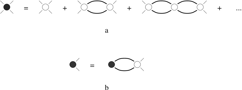
Figure 1: a) Ladder diagrams. b) BS equation.

The two-particle bound state manifests itself as a pole in the four-point function. The pole arises after summation of the ladder diagrams (Fig. 1a). Each ladder diagram develops a kinematic singularity when the momentum flowing through the diagram is near the two-particle threshold: $p^{2}\approx-4m^{2}$, since the momentum integration in each loop then contains a region where two of the intermediate states simultaneously go on-shell and the propagators in the loop integral simultaneously have poles. This singularity produces large logarithms that compensate for powers of the coupling, so near the threshold all ladder diagrams are of the same order. The vertices in Fig. 1a correspond to the sum of the two-particle irreducible (2PI) diagrams, that is, the diagrams that cannot be split into disconnected pieces by cutting two internal lines whose total momentum is $p$. 2PI diagrams are analytic at the two-particle threshold in the $s$-channel.

The position of the pole is determined by the BS equation, graphically represented in Fig. 1b. The BS equation is the homogeneous part of the Dyson equation for ladder diagrams [7]:

$$\Gamma(p_{1},p_{2})=\int\frac{d^{3}q}{(2\pi)^{3}}\,\Gamma(q,p-q)G(q)K(q,p-q;p_{1},p_{2})G(p-q),~{}~{}~{}~{}p=p_{1}+p_{2}.$$ (2.5)

Here, $G$ is the propagator and $K$ is the BS kernel, the aforementioned sum of 2PI diagrams. The BS equation is a linear eigenvalue problem for the wave function $\Gamma$ and the bound state mass:

$$M^{2}\equiv-p^{2}.$$ (2.6)

We take:

$$M=(2-\Delta)m,$$ (2.7)

where $\Delta$ is small.

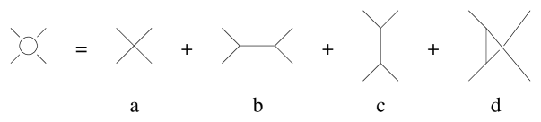
Figure 2: Tree-level BS kernel.

To the leading order in $g/m$, the BS kernel is given by the sum of three diagrams in Fig. 2. The diagram $a$ contributes $-g/2$ to the kernel:

$$K_{a}=-\frac{g}{2}.$$

The diagram $b$ gives

$$K_{b}=\frac{3gm^{2}}{2}\,\frac{1}{m^{2}-M^{2}}=-\frac{g}{2}+O(\Delta).$$

The contribution of the diagrams $c$ and $d$ depends on the momentum transfer in the $t$ and $u$ channels. However, the momentum transfer is very small when external momenta and both of the propagators in (2.5) are on shell: simple kinematic arguments show that the typical momentum in the $t$ or $u$ channel propagators is of order $\Delta m$. To the first approximation, we can just set it to zero:

$$K_{c}=\frac{3gm^{2}}{2}\,\frac{1}{(p_{1}-q)^{2}+m^{2}}\approx\frac{3g}{2}\,,$$

$$K_{d}=\frac{3gm^{2}}{2}\,\frac{1}{(p_{2}-q)^{2}+m^{2}}\approx\frac{3g}{2}\,.$$

Collecting all three terms together, we get:

$$K=2g.$$ (2.8)

The kernel corresponds to a local four-point interaction in this approximation. The effective quartic coupling appears to be negative. This happens because the exchange diagram $c$ dominates over the pure four-point vertex $a$ and the annihilation graph $b$, so the interaction is attractive. No matter how weak the interaction is, it will bind elementary quanta into bound states.

Since the binding energy is small, the non-relativistic approximation should be valid at small $g/m$. The non-relativistic limit of the BS equation with the positive local kernel is the two-body Schrödinger equation with attractive $\delta$-function potential. This quantum-mechanical problem has a bound state at any value of the coupling with exponentially small binding energy [8]. An approach based on the non-relativistic approximation was elaborated in [4]. This approach is simple and physically transparent, but it only allows us to find the binding energy up to a numerical factor. Here we follow a more systematic route based on the full BS equation.

The BS equation with the local kernel Eq. (2.8) corresponds to summing an infinite series of bubble diagrams, and can be written as

$$1=2g\int\frac{d^{3}q}{(2\pi)^{3}}\,\frac{1}{(q^{2}+m^{2})[(p-q)^{2}+m^{2}]}.$$ (2.9)

Evaluating the integral,

$$\int\frac{d^{3}q}{(2\pi)^{3}}\frac{1}{(q^{2}+m^{2})[(p-q)^{2}+m^{2}]} = \frac{\arcsin\left(\sqrt{\frac{p^{2}}{4m^{2}+p^{2}}}\right)}{4\pi\sqrt{p^{2}}}=\frac{\ln\left(\frac{2m+M}{2m-M}\right)}{8\pi M}$$ (2.10)

$$= \frac{\ln\left(\frac{4}{\Delta}\right)}{16\pi m}+O(\Delta\ln\Delta),$$

we obtain:

$$1=2g\frac{\ln\left(\frac{4}{\Delta}\right)}{16\pi m}.$$ (2.11)

This equation predicts an exponentially small binding energy:

$$\Delta={\rm const}\cdot\exp\left(-\frac{8\pi m}{g}\right),$$ (2.12)

in accord with the result obtained in the non-relativistic approximation [4].

The normalization of the binding energy cannot be deduced from Eq. (2.11). We cannot keep the constant term in (2.10), because it has the same magnitude as logarithmic terms in the next order of perturbation theory, which are proportional to $g^{2}/m^{2}\ln\Delta\sim g/m$. There are other sources of corrections of order $g/m$, as well. We need to compute all of them to fix the normalization of the binding energy.

2.2 Corrections to propagator

Figure 3: One-loop corrections to the propagator.

One-loop corrections to the propagator are given by three diagrams in Fig. 3. They shift the pole of the propagator to

$$\mu^{2}=m^{2}-\frac{3gm}{16\pi}\ln 3-g\Lambda,$$ (2.13)

where by $\Lambda$ we denote the linearly divergent integral

$$\Lambda\equiv\int\frac{d^{3}q}{(2\pi)^{3}}\,\frac{1}{q^{2}+m^{2}}.$$ (2.14)

Expanding the third diagram in Fig. 3 near the mass shell, we get:

$$G^{-1}(k)=(p^{2}+\mu^{2})\left[1+\left(3-\frac{9}{4}\ln 3\right)\frac{g}{24\pi m}\right]+O\Bigl{(}(p^{2}+\mu^{2})^{2}\Bigr{)}$$ (2.15)

and

$$G(k)=\frac{1}{p^{2}+\mu^{2}}\,\left[1-\left(3-\frac{9}{4}\,\ln 3\right)\frac{g}{24\pi m}\right]+O(1).$$ (2.16)

In evaluating the integral (2.10), the corrections to the propagator will result in the replacement of the bare mass $m$ by the renormalized (physical) mass $\mu$ and in the multiplication of the whole integrand by the wave function renormalization factor.

It is natural to express everything in terms of the physical mass gap (2.13). In particular, we set:

$$M=(2-\Delta)\mu.$$ (2.17)

This definition affects the BS kernel, since the contribution of the diagram $b$ in Fig. 2 depends on how exactly we define $M$:

$$K_{b} = \frac{3gm^{2}}{2}\frac{1}{m^{2}-M^{2}}=\frac{3g}{2}\frac{m^{2}}{\mu^{2}-M^{2}}\left[1-\left(\frac{3gm}{16\pi}\,\ln 3+g\Lambda\right)\frac{1}{\mu^{2}-M^{2}}\right]$$ (2.18)

$$= -\frac{g}{2}-\frac{g^{2}}{8\pi m}\ln 3-\frac{2g^{2}\Lambda}{3m^{2}}+O(\Delta)+O(g^{3}).$$

This differs from the result based on our previous definition by an amount

$$\delta K_{b}=-\frac{g^{2}\ln 3}{8\pi m}-\frac{2g^{2}\Lambda}{3m^{2}}.$$ (2.19)

2.3 One-loop corrections to the kernel

Figure 4: One-loop two-particle-irreducible diagrams.

The one-loop corrections to the kernel of the BS equations are given by thirteen diagrams in Fig. 4. Since we are interested only in the logarithmically enhanced terms in the BS equation, all these diagrams can be evaluated on shell and at zero momentum transfer in the $t$ and $u$ channels.

The linearly divergent diagrams 1-3 sum up to zero:

$$\delta K_{1-3}=0.$$ (2.20)

The diagrams 4-7 cancel the divergence in the diagram $b$, the second term in Eq. (2.19):

$$\delta K_{4-7}=\frac{2g^{2}\Lambda}{3m^{2}}.$$ (2.21)

All linear divergences eventually have canceled. It is satisfying to see that the net one-loop contribution to the kernel is finite, as it should be.

The remaining diagrams give:

$$\delta K_{8-13}=(9-6+1+12-4+2)\frac{g^{2}}{16\pi m}=7\,\frac{g^{2}}{8\pi m}.$$ (2.22)

Collecting together the contributions (2.19)–(2.22) we get the one-loop correction to the BS kernel:

$$\delta K=(7-\ln 3)\frac{g^{2}}{8\pi m}.$$ (2.23)

2.4 Momentum dependence

Finally, we consider the most subtle corrections that come from the momentum dependence of the kernel and of the wave function. Those were neglected in the leading order calculation because the logarithmic enhancement of the bubble diagram near threshold comes from the region of integration in (2.5) where all momenta are almost on shell. This allowed us to forget about the momentum dependence of the wave function and to set it to one. In fact, we can always require that the wave function is equal to the one on shell. This can be regarded as a normalization condition. But to compute non-logarithmic terms we need to know the complete off-shell wave function.

Once the on-shell condition on the external momenta $p_{1},p_{2}$ is relaxed, we can no longer neglect the momentum transfer in the diagrams $c$ and $d$ in Fig. 2. The BS equation then gives:

$$\Gamma(p_{1},p_{2}) = \int\frac{d^{3}q}{(2\pi)^{3}}\,\frac{1}{(q^{2}+m^{2})[(p-q)^{2}+m^{2}]}\left[\frac{3gm^{2}}{(q-p_{1})^{2}+m^{2}}-g\right]$$ (2.24)

$$= \frac{g}{8\pi m}\,\ln\left(\frac{1}{\Delta}\right)\left(\frac{3m^{2}}{4m^{2}+p_{1}^{2}+p_{2}^{2}}-\frac{1}{2}\right)$$

$$= \frac{3m^{2}}{4m^{2}+p_{1}^{2}+p_{2}^{2}}-\frac{1}{2}+O\left(\frac{g}{m}\right).$$

2.5 Next-to-leading order BS equation

With all corrections taken into account, the BS equation reads:

$$1 = \left[1-\left(3-\frac{9}{4}\,\ln 3\right)\frac{g}{24\pi\mu}\right]^{2}$$ (2.25)

$$\times\int\frac{d^{3}q}{(2\pi)^{3}}\,\left[\frac{3\mu^{2}}{4\mu^{2}+p^{2}+(p-q)^{2}}-\frac{1}{2}\right]\frac{1}{(q^{2}+\mu^{2})[(p-q)^{2}+\mu^{2}]}$$

$$\times\left[\frac{3g\mu^{2}}{(q-p_{1})^{2}+m^{2}}-g+(7-\ln 3)\frac{g^{2}}{8\pi\mu}\right],$$

where external momenta $p_{1}$ and $p_{2}$ are on shell: $p_{1,2}^{2}=-\mu^{2}$. We need to retain terms of order $g/\mu$ and $(g^{2}/\mu^{2})\ln\Delta$ on the right hand side. For this reason, $O(g/m)$ corrections to the wave function can be neglected, since they vanish on shell and therefore do not lead to the logarithmic enhancement. The loop integrals encountered in (2.25) are listed in Appendix and in (2.10). Using these results, we get after a little of algebra:

$$\log\Delta=-\frac{8\pi\mu}{g}+2\log 2-\frac{1}{2}\log 3+O\left(\frac{g}{\mu}\right)$$ (2.26)

that is

$$\Delta=\frac{4}{\sqrt{3}}\exp\left(-\frac{8\pi\mu}{g}\right).$$ (2.27)

2.6 Comparison with numerical results

To compare Eq. (2.26) with numerical results one has to know a value for the dimensionless coupling $\hat{u}\equiv g/\mu$. The safest thing to do is to relate $\hat{u}$ to the renormalized coupling $u_{R}$ defined e.g. as in Ref.[18], whose critical value is precisely known from Monte Carlo simulations [13]

$$u_{R}=14.3(1)$$ (2.28)

in terms of $u_{R}$ we have, using results from [3, 18]

$$\hat{u}=u_{R}\left[1+u_{R}\left(\frac{15}{128\pi}+\frac{3\log 3}{32\pi}\right)\right]$$ (2.29)

so that

$$\log\Delta=-\frac{8\pi}{u_{R}}+\left(\frac{15}{16}+\frac{\log 3}{4}+2\log 2\right)+O(u_{R})$$ (2.30)

Therefore the leading-order result is

$$\log\Delta=-\frac{8\pi}{u_{R}}=-1.76(2)$$ (2.31)

corresponding to

$$\Delta=0.172(3).$$ (2.32)

This result is compatible with the assumption of weak binding energy that underlies the Bethe-Salpeter formalism, and is in a very good agreement with the numerical result,

$$\Delta_{MC}=0.17(3).$$ (2.33)

However, the parameter of expansion in perturbation theory is comparatively large, and the NLO correction is not small: the $O(1)$ contribution to $\log\Delta$ is $\sim 2.6$, that is actually greater than the LO contribution. Therefore a reliable estimate of the subleading corrections to the binding energy seems to require the computation of a large number of terms in perturbative series, so as to make a resummation possible, which is typical for application of $3d$ $\phi^{4}$ theory to critical phenomena.

3 Dependence on the magnetic field

It is possible to study the dependence of the bound state masses on the magnetic field. Because the magnetic field couples to the order parameter, we know how to introduce it in the effective description in terms of $\phi^{4}$ theory. We can take the magnetic field into account by adding a linear term to the action:

$$S=\int d^{3}x\left[\frac{1}{2}\partial_{\mu}\phi\ \partial_{\mu}\phi+\frac{g}{4!}(\phi^{2}-v^{2})^{2}-h\phi\right].$$ (3.34)

The magnetic field shifts the minimum of the potential, which now is determined by the equation

$$\frac{g}{6}\,\phi_{0}(\phi_{0}^{2}-v^{2})=h.$$ (3.35)

Expanding the order parameter around $\phi_{0}$,

$$\phi=\phi_{0}+\varphi,$$ (3.36)

we get for the action:

$$S=\int d^{3}x\left[\frac{1}{2}\partial_{\mu}\varphi\ \partial_{\mu}\varphi+\frac{1}{2}m^{2}_{h}\varphi^{2}+\frac{1}{3!}\,g_{3}\varphi^{3}+\frac{1}{4!}\,g\varphi^{4}\right]+S_{0},$$ (3.37)

where the mass and the trilinear coupling are

$$m^{2}_{h}=\frac{g}{6}\,(3\ \phi_{0}^{2}-v^{2}),$$ (3.38)

$$g_{3}=g\ \phi_{0}.$$ (3.39)

The sum of the diagrams in Fig. 2 gives the tree-level BS kernel:

$$K_{h}=\frac{g_{3}^{2}}{m^{2}_{h}}+\frac{g_{3}^{2}}{2}\,\frac{1}{m_{h}^{2}-4m^{2}_{h}}-\frac{g}{2}=g\,\frac{7\phi_{0}^{2}+v^{2}}{6\phi_{0}^{2}-2v^{2}}.$$ (3.40)

Repeating the same steps as we used to calculate the binding energy at zero magnetic field, we get

$$\Delta={\rm const}\,\exp\left(-\frac{16\pi m_{h}}{K_{h}}\right),$$ (3.41)

where $\Delta$ is the dimensionless binding energy: $M_{h}=(2-\Delta)m_{h}$.

It is useful to introduce the dimensionless variable

$$\xi=\frac{\phi_{0}}{v},$$ (3.42)

which satisfies the equation

$$\xi^{3}-\xi=\frac{6}{gv^{3}}\,h=\frac{2}{m^{3}}\sqrt{\frac{g}{3}}\,h.$$ (3.43)

The binding energy is expressed in terms of $\xi$ and $m$, the mass at zero magnetic field, as

$$\Delta={\rm const}\,\exp\left(-\frac{8\pi m}{g}\,\frac{(6\xi^{2}-2)^{3/2}}{7\xi^{2}+1}\right).$$ (3.44)

It is easy to see that $\Delta$ is a decreasing function of $h$. Thus the magnetic field loosens the binding of composite states and shifts their masses closer to the threshold.

4 Duality and the spectrum of Ising systems

The $3D$ Ising model and ${\mathbb{Z}}_{2}$ gauge theory are related by an exact duality transformation. The broken symmetry phase of the spin model is mapped into the confining phase of the gauge theory. The purpose of this section is to show that, in this phase, the duality relationship implies an exact coincidence of the spectra of the two theories. The proof relies on the existence of a non-zero interface tension and therefore applies exclusively to the broken symmetry phase of the spin model.

There are several books and reviews which discuss duality in spin systems and in particular in Ising-type models (see e.g. Ref. [9]). However the duality transformation is usually treated in the thermodynamic limit only, while to study the spectrum of the transfer matrix it is necessary to extend the analysis to finite lattices. This is possible as long as one carefully takes into account all possible boundary conditions.

The novel feature of our approach, which greatly simplifies the whole analysis, is the use of the Transfer Matrix (TM) formalism. Let us first recall the definitions of the lattice models we are concerned with, and the notion of duality in the thermodynamic limit.

• The spin Ising model

  The Ising model is defined by the action

  $$S_{spin}=-\beta_{spin}\sum_{\langle n,m\rangle}s_{n}s_{m}\;,$$ (4.45)

  where the field variable $s_{n}$ takes the values $-1$ and $+1$; $~{}~{}n\equiv(n_{0},n_{1},n_{2})$ labels the sites of a simple cubic lattice of size $L_{0}$, $L_{1}$ and $L_{2}$ in the three directions. The notation $\langle n,m\rangle$ in Eq. (4.45) indicates that the sum is taken over pairs of nearest neighbor sites only.

• The gauge Ising model

  The building blocks of the ${\mathbb{Z}}_{2}$ gauge model are the link variables $g_{n;\mu}\in\{-1,1\}$, which play the role of gauge fields. Denoting by $\mu$ the direction of the link, the action is

  $$S_{gauge}=-\beta\;\;\sum_{n,\mu<\nu}\;\;g_{n;\mu\nu}$$ (4.46)

  where $g_{n;\mu\nu}$ are the plaquette variables, defined by

  $$g_{n;\mu\nu}=g_{n;\mu}\;g_{n+\mu;\nu}\;g_{n+\nu;\mu}\;g_{n;\nu}~{}~{}~{}.$$ (4.47)

  This action is invariant under local ${\mathbb{Z}}_{2}$ gauge transformations defined as follows: one chooses arbitrarily a subset of the sites of the lattice and changes signs of all variables defined on the links which end on these sites (if two neighboring sites belong to the chosen subset the link that joins them is changed twice, that is not changed). It is immediately clear that the plaquette values, like any other product of links along a closed path, are invariant under this gauge transformation. For more details about this model, see e.g. Ref. [10].

• Duality

  There is an exact duality transformation which relates the Ising model and the ${\mathbb{Z}}_{2}$ gauge model. This transformation is known as Kramers–Wannier duality. It relates the partition functions of the two models evaluated at two different values of the coupling constants:

  $$Z_{gauge}(\beta)~{}\propto~{}Z_{spin}(\tilde{\beta})$$

  $$\tilde{\beta} = -\frac{1}{2}\log\left[\tanh(\beta)\right]\ ,$$ (4.48)

  where $\tilde{\beta}$ will be denoted as the “dual coupling” in what follows.

  It is easy to see that low values of $\beta$ are mapped into high values of $\tilde{\beta}$ and vice versa. Thus the confining region of the gauge theory is mapped into the broken symmetry phase of the spin model. In particular the end points of these two phases, the deconfinement transition and the magnetization transition, are mapped into each other.

An important feature of the dual transformation on a lattice of finite size is that it does not conserve the boundary conditions (BC). In the thermodynamic limit this fact becomes irrelevant, but on lattices of finite extent it cannot be neglected. In particular the ${\mathbb{Z}}_{2}$ gauge model with periodic BC in all directions is mapped by duality into the Ising spin model with fluctuating BC, so that the partition function is given by the sum of the partition functions with all possible choices of periodic ($p$) or antiperiodic ($a$) BC:

$$Z_{gauge,ppp}(\beta)=\frac{1}{2}c^{V}(Z_{spin,ppp}(\tilde{\beta})+Z_{spin,ppa}(\tilde{\beta})+...+Z_{spin,aaa}(\tilde{\beta})~{}),$$ (4.49)

where $V\equiv L_{0}L_{1}L_{2}$ is the volume of the lattice, and $c$ is a constant which can be easily evaluated, but is irrelevant for our purposes.

This result is discussed in full generality (for a generic lattice geometry and symmetry group) in [11]. In the particular case of the Ising model on a cubic lattice it can be easily obtained by a direct implementation of the duality transformation.

Let us now consider the duality transformation in the framework of the transfer matrix approach. The $0$ direction will be our “time”. If we choose periodic BC in the $0$ direction without specifying the BC in the $1$ and $2$ directions we obtain:

$$Z_{spin,pxy}=\mbox{tr}({\bf T_{xy}})^{L_{0}},$$ (4.50)

where ${\bf T}_{xy}$ denotes the transfer matrix of the model in which $x,y\in\{a,p\}$ BC are chosen in the 1 and 2 directions respectively.

The antiperiodic BC in the $0$ direction can be obtained by acting with a spin–flip operator ${\bf P}$, which changes the sign of all spins in a given time slice. Thus we may write

$$Z_{spin,axy}=\mbox{tr}{\bf P}({\bf T}_{xy})^{L_{0}}.$$ (4.51)

Since the operators ${\bf T}_{xy}$ and ${\bf P}$ commute, they have a common set of eigenfunctions. Let us denote the eigenvalues of ${\bf T}_{xy}$ by $\lambda_{xy,i}$ and those of ${\bf P}$ by $p_{i}$. The possible values of $p_{i}$ are $1$ and $-1$. States that are symmetric in the magnetization have $p_{i}=1$ and those that are antisymmetric have $p_{i}=-1$.

Thus we can write

$$Z_{spin,pxy}+Z_{spin,axy}=\mbox{tr}(1+{\bf P})({\bf T}_{xy})^{L_{0}}=2\sum_{i,sym}\lambda_{xy,i}^{L_{0}},$$ (4.52)

where $\sum_{i,sym}$ means that the sum is restricted to the states that are symmetric in the magnetization (See Ref. [12] for further details on this type of construction).

Using this result we can write the duality relation in terms of the transfer matrix eigenvalues:

$$\sum_{j}\gamma_{j}^{L_{0}}=c^{L_{0}L_{1}L_{2}}\left[\sum_{i,sym}\lambda_{pp,i}^{L_{0}}+\sum_{i,sym}\lambda_{pa,i}^{L_{0}}+\sum_{i,sym}\lambda_{ap,i}^{L_{0}}+\sum_{i,sym}\lambda_{aa,i}^{L_{0}}\right],$$ (4.53)

where $\gamma_{j}$ are the eigenvalues of the transfer matrix of the gauge system.

It is instructive to show explicitly that the sums on the two sides of Eq. (4.53) have the same number of terms. On the spin side (right hand side of Eq. (4.53)) we have $2^{L_{1}L_{2}-1}$ terms for each sector. In fact, the transfer matrix is a $2^{L_{1}L_{2}}\times 2^{L_{1}L_{2}}$ matrix, but only half of the eigenvalues fulfil the symmetry requirement. Thus taking together all the four sectors we end up with a sum of $2^{L_{1}L_{2}+1}$ terms. On the gauge side we have $2L_{1}L_{2}$ link variables, but we may fix the gauge. The maximum number of gauge variables that we may fix, in order to preserve the periodic BC, is exactly $L_{1}L_{2}-1$. This is easy to see: we may fix, say, all the links in the $1$ direction except those in the last row, where we may fix all the links in the $2$ direction, except the last one. Thus we end up with only $L_{1}L_{2}+1$ degrees of freedom left. Hence the corresponding transfer matrix has $2^{L_{1}L_{2}+1}$ eigenvalues, that is exactly the same number as for the spin model.

Since for finite values of $L_{1}$ and $L_{2}$ the two sums contain a finite number of terms and since Eq. (4.53) holds for any integer $L_{0}$, each $\gamma_{j}$ has to have an exact (up to an overall factor $c^{L_{1}L_{2}}$) counterpart in the left hand side of the equation. The overall factor cancels when one takes the ratios of all the eigenvalues to the lowest one to obtain the physical spectrum, and so the latter coincides in the two models.

However our goal is to compare the spectra of the gauge theory and the spin model both with periodic BC in all directions, while Eq. (4.53) involves a sum over many different choices of the spin model BC. Therefore we must find a relationship between the $\lambda_{pp,i}$ eigenvalues and those belonging to the other three sectors. This is easily done by noticing that in the low temperature phase of the Ising model with antiperiodic boundary conditions at least one interface has to be created in the system. Therefore at leading order (neglecting the cases in which more than one interface appear):

$$Z_{ppa}\approx\exp(-\sigma\;L_{0}L_{1})\;Z_{ppp},$$ (4.54)

where $\sigma$ is the interface tension.

For the transfer matrix eigenvalues this gives

$$\lambda_{pp,max}\approx\exp(\sigma L_{1})\;\lambda_{pa,max}$$ (4.55)

where, with the notation $\lambda_{pp,max}$ we denote the low lying states of the spectrum.

So we can conclude that for sufficiently large $L_{1}$ and $L_{2}$, the low lying spectrum of the $Z_{2}$ gauge theory in the confining phase with periodic boundary conditions coincides with the symmetric sector of the Ising spin model spectrum in the low temperature phase with periodic boundary conditions only. (This last argument was already presented in [13]).

5 The dual bound state picture of glueballs in ${\mathbb{Z}}_{2}$ gauge theory

In this section we show that the interpretation of the spectrum of three-dimensional models in the universality class of the $3D$ Ising model as bound states of the elementary quanta provides an analytical tool to explain the qualitative features of the glueball spectrum of ${\mathbb{Z}}_{2}$ gauge theory, and especially its angular momentum dependence.

Consider first the spin Ising model in the low-temperature region. Here the existence of bound states can be immediately inferred from the diagrammatics of the low-temperature expansion. This was shown in [14] for the $4D$ case, where however all bound states are expected to disappear in the continuum limit due to triviality.

The mechanism is very simple, and is best explained in the transfer matrix formalism. As discussed in [15, 16], to the leading order in the low-temperature expansion of the transfer matrix, all time slices are forced to have the same configuration of spins, and the the eigenvectors are given by all the possible spin configurations in a single time slice. The eigenvalues of the Hamiltonian (that is minus the logarithm of the transfer matrix) are given by the energy of each configuration.

The ground state then corresponds to the configuration in which all the spins on any time slice are parallel; the first excited state corresponds to one flipped spin, which requires four bonds to be frustrated. To proceed, one has to flip two spins: if these are chosen in non-neighboring sites, the energy is just twice the one of the first excitation, since eight bonds will be frustrated. However one can flip two neighboring spins at the cost of frustrating six bonds only: the corresponding state is a bound state of the fundamental excitation, with mass just below the two-particle threshold.

One can also construct states of given angular momentum and parity by choosing linear combinations of time slice configurations with nontrivial transformation properties under spatial rotations and parity reflections. This can be done systematically by using standard group theory results, namely the theory of representations of the dihedral group $D^{4}$, which is the relevant group on a square lattice. This analysis is performed in Ref. [17], to which we refer for details.

The important point is that any given angular momentum requires a certain minimum number $n_{c}$ of spin flips. This means that a bound state of such angular momentum will be composed of at least $n_{c}$ elementary quanta. In Tab. 1 we have reported the values of $n_{c}$ for the various values of the angular momentum. For example, Fig. 5 shows the simplest lattice operator corresponding to angular momentum $J=2$ and parity $P=-1$, which requires $n_{c}=3$ elementary quanta, while Fig. 6 shows how states with quantum numbers $J=0,2$ and $P=+,-$ can be constructed with four elementary quanta. If we assume that the binding energy is always much smaller that the common mass of the elementary constituents of the bound states, we end up with a prediction for the angular momentum dependence of the glueball spectrum of the ${\mathbb{Z}}_{2}$ gauge theory in the strong coupling regime.

It is not at all guaranteed, of course, that the spectrum will retain these same features when going from the strong coupling regime to the scaling region: however the data from Monte Carlo simulations of the gauge theory show that this is actually the case. The third column of Tab. 1 contains the Monte Carlo results for the glueball masses (from Ref. [17]), normalized to the mass of the lowest glueball. This shows that our dual bound state picture indeed explains the peculiar qualitative features of the glueball spectrum.

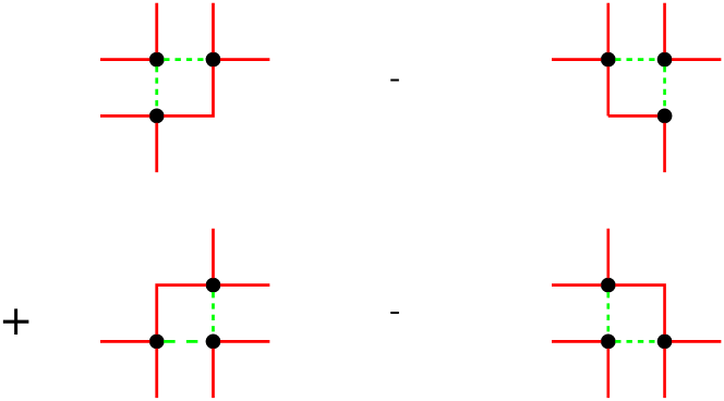
Figure 5: Three elementary quanta are required to construct a state with quantum numbers $2^{-}$. Dots represent flipped spins, solid lines are frustrated links, dashed lines satisfied links.

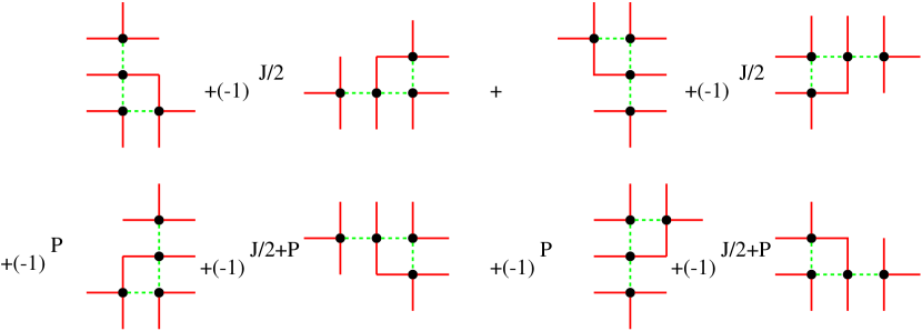
Figure 6: Bound states of $n_{c}=4$ elementary quanta.

Table 1: The bound states that can be constructed with $n_{c}$ elementary quanta are classified in terms of their angular momentum and parity. The last column shows the mass of the corresponding glueball state in ${\mathbb{Z}}_{2}$ gauge theory.

$n_{c}$	$J^{P}$	$m(J^{P})/m(0^{+})$
1	$0^{+}$	1
2	$0^{+*}$	1.88(2)
3	$0^{+**}$	2.59(4)
	$2^{\pm}$	2.59(4)
4	$2^{\pm*}$	3.23(7)
	$0^{-}$	3.24(16)
5	$0^{-*}$	4.48(20)
	$1^{\pm}$	4.12(17)

In particular, some characteristic approximate degeneracies in the spectrum find a natural explanation in this picture: for example the states $0^{+,**}$ and $2^{\pm}$ are nearly degenerate because they are both bound states of $n_{c}=3$ elementary constituents. Bound states of $n_{c}=4$ constituents give rise to the $0^{-}$ and $2^{\pm,*}$ states, again explaining their near degeneracy, and the same applies to $0^{-,*}$ and $1^{\pm}$ when interpreted as $n_{c}=5$ bound states. We do not expect these degeneracies to be exact, since there is no reason to expect the binding energies to be exactly the same for bound states of different angular momentum.

Once the minimum number $n_{c}$ of constituents for a given value of the angular momentum has been reached, it is easy to see that states with the same angular momentum can be constructed out of any number $n>n_{c}$ of constituents. This suggests that the approximate degeneracies just discussed appears between pairs of states only because, in general, only two states can be detected with numerical methods in each channel. It is very likely that the degeneracies actually group together larger and larger sets of states as the number of constituents is increased. For example, we might conjecture that the states $0^{-,*}$ and $1^{\pm}$ ($n_{c}=5$) are nearly degenerate with the (as yet undetected) states $0^{+,****}$, $2^{\pm,**}$. This degeneracy pattern is a prediction of the dual bound state picture of glueballs.

6 Summary and further developments

The broken symmetry phase of $3D$ models with ${\mathbb{Z}}_{2}$ symmetry shows a rich spectrum of massive excitations, contrary to naive expectations based on the perturbative field-theoretical treatment. The non-perturbative states in the spectrum can be interpreted as bound composites of the elementary particle excitation. When applied to $3D$ ${\mathbb{Z}}_{2}$ gauge theory, this approach gives a nice explanation of the angular momentum dependence of the glueball spectrum. In particular, an observed rather peculiar degeneracy pattern naturally arises in the bound-state interpretation.

It would be interesting to consider the contribution of the bound states to universal amplitude ratios. The obvious way to do that is to use the ladder approximation for correlation functions, which incorporates all diagrams that blow up near the two-particle threshold. It would be also interesting to understand if there are bound states in the systems with $N>1$ order parameters. The physics is completely different in this case because the dominating forces are long-range due to the Goldstone bosons of the broken $O(N)$ symmetry.

Acknowledgements

K.Z. would like to thank P. Simon for discussions. The work of K.Z. was supported by NSERC of Canada, by Pacific Institute for the Mathematical Sciences and in part by RFBR grant 98-01-00327 and RFBR grant 00-15-96557 for the promotion of scientific schools.

Appendix A

$$\int\frac{d^{3}q}{(2\pi)^{3}}\,\frac{1}{[4\mu^{2}+q^{2}+(p-q)^{2}](q^{2}+m^{2})[(p-q)^{2}+m^{2}]}=\frac{1}{32\pi\mu^{3}}\,\ln\left(\frac{4}{9\Delta}\right).$$ (A.1)

$$\int\frac{d^{3}q}{(2\pi)^{3}}\,\frac{1}{(q^{2}+m^{2})[(p-q)^{2}+m^{2}][(q-p_{1})^{2}+m^{2}]}=\frac{1}{16\pi\mu^{3}}\,\ln\left(\frac{4}{9\Delta}\right).$$ (A.2)

$$\int\frac{d^{3}q}{(2\pi)^{3}}\, \frac{1}{[4\mu^{2}+q^{2}+(p-q)^{2}](q^{2}+m^{2})[(p-q)^{2}+m^{2}][(q-p_{1})^{2}+m^{2}]}$$ (A.3)

$$=\frac{1}{32\pi\mu^{5}}\,\left[\ln\left(\frac{4}{9\Delta}\right)-\frac{2}{3}\right].$$

All integrals are calculated on shell: $p_{1,2}^{2}=-\mu^{2}$, and near the two-particle threshold: $p^{2}\equiv(p_{1}+p_{2})^{2}=-M^{2}=(2-\Delta)^{2}\mu^{2}$.

References

- [1] C. Itzykson and J. M. Drouffe, Statistical Field Theory, (University Press, Cambridge, 1989).
- [2] J. Zinn-Justin, Quantum Field Theory And Critical Phenomena, (Clarendon, Oxford, 1989).
- [3] M. Caselle, M. Hasenbusch and P. Provero, Nucl. Phys. B556 (1999) 575 [hep-lat/9903011].
- [4] M. Caselle, M. Hasenbusch, P. Provero and K. Zarembo, Phys. Rev. D62 (2000) 017901 [hep-th/0001181].
- [5] D. Lee, N. Salwen and M. Windoloski, hep-lat/0010039.
- [6] R. F. Dashen, B. Hasslacher and A. Neveu, Phys. Rev. D11 (1975) 3424.
- [7] V. B. Berestetsky, E. M. Lifshits and L. P. Pitaevsky, “Quantum Electrodynamics”, Pergamon, Oxford 1982.
- [8] C. Thorn, Phys. Rev. D19 (1979) 639.
- [9] R. Savit, Rev. Mod. Phys. 52 (1980) 453.
- [10] J. Drouffe and J. Zuber, Phys. Rept. 102 (1983) 1.
- [11] C.Gruber, A.Hintermann and D.Merlini, Group Analyisis of Classical Lattice Systems, (Springer-Verlag, Berlin-Heidelberg-New York, 1977).
- [12] M. Caselle, R. Fiore, F. Gliozzi, M. Hasenbusch, K. Pinn and S. Vinti, Nucl. Phys. B432 (1994) 590 [hep-lat/9407002].
- [13] M. Caselle and M. Hasenbusch, Nucl. Phys. B470 (1996) 435 [hep-lat/9511015].
- [14] M. Lüscher and P. Weisz, Nucl. Phys. B295 (1988) 65.
- [15] M. E. Fisher and W. J. Camp, Phys. Rev. Lett. 26 (1971) 565.
- [16] W. J. Camp, Phys. Rev. B7 (1973) 3187.
- [17] V. Agostini, G. Carlino, M. Caselle and M. Hasenbusch, Nucl. Phys. B484 (1997) 331 [hep-lat/9607029].
- [18] G. Münster and J. Heitger, Nucl. Phys. B424 (1994) 582 [hep-lat/9402017].