Phase structure of a compact $\bm{U(1)}$ gauge theory
from the viewpoint of a sine-Gordon model

Abstract

We discuss the phase structure of the four-dimensional compact $U(1)$ gauge theory at finite temperature using a deformation of the topological model. Its phase structure can be determined by the behavior of the Coulomb gas (CG) system on the cylinder. We utilize the relation between the CG system and the sine-Gordon (SG) model, and investigate the phase structure of the gauge theory in terms of the SG model. Especially, the critical-line equation of the gauge theory in the strong-coupling and high-temperature region is obtained by calculating the one-loop effective potential of the SG model.

I Introduction

Recently the scenario of treating a gauge theory as a deformation of the topological model has been proposed by several authors kondo ; HT ; izawa . The motivation of this scenario is to investigate the confinement and the phase structure at zero temperature or finite temperature. In particular, we can calculate the expectation value of the Wilson loop (at zero temperature) or Polyakov loop (at finite temperature) by considering the topological model and so derive the linear potential, which means the quark confinement wilson . The Parisi-Sourlas (PS) dimensional reduction PS is very powerful to study the topological model. This scenario can be also applied to a compact $U(1)$ gauge theory. It is quite related to QCD by the use of the Abelian projection, which is a partially gauge fixing method tHooft ; kondo2 . In the case of the compact $U(1)$ gauge theory the topological model becomes the two-dimensional $O(2)$ nonlinear sigma model (NLSM₂) and we can show that the confining phase exists in the strong-coupling region at zero temperature and finite temperature qed ; KY2 .

In the case of zero temperature, the confining-deconfining phase transition of the compact $U(1)$ gauge theory can be described by the Berezinskii-Kosterlitz-Thouless (BKT) phase transition BKT in the $O(2)$ NLSM₂ qed . It is well known that the $O(2)$ NLSM₂ has vortex solutions and is equivalent to several models, such as the Coulomb gas (CG) system, sine-Gordon (SG) model and massive Thirring (MT) model. In the compact $U(1)$ gauge theory the confining phase exists at the strong-coupling region due to the effect of the vortex solution, which induces the linear potential between the static charged test particles. The confining phase transition corresponds to the BKT phase transition in the CG system BKT , or the Coleman transition in the SG model Coleman . The CG system has a phase transition from a dipole phase to a plasma phase. The quantum SG model undergoes a phase transition from a stable vacuum to an unstable vacuum at the certain critical coupling. Both phase transitions are intimately connected through the equivalence between the CG system and the SG model.

In our previous papers KY2 ; KY , we have investigated the phase structure of the compact $U(1)$ gauge theory at finite temperature from the viewpoint of the behavior of the CG system on the cylinder. In particular, we could study its strong-coupling and high-temperature region by using the behavior of the one-dimensional CG system 1C . This result is consistent with the prediction in Ref. SV .

In this paper we would like to investigate the phase structure of the compact $U(1)$ gauge theory at finite temperature more quantitatively from the different aspect. We investigate its phase structure from the viewpoint of the SG model by the use of relationship the CG system and the SG model. The one-loop effective potential of the SG model enables us to investigate the phase structure of the gauge theory at the high-temperature and strong-coupling region. Especially, we can evaluate the critical-line equation.

Our paper is organized as follows. Section II is devoted to a review of a deformation of a topological model. In Sec. III we discuss the equivalence between the thermal SG model and the CG system on the cylinder. In Sec. IV the one-loop effective potential of the SG model is discussed. Especially, the critical-line equation of the SG model can be obtained. We can evaluate the critical-line equation of the compact $U(1)$ gauge theory at finite temperature from this result. Section V is devoted to the conclusion and discussion.

II Compact $\bm{U(1)}$ gauge theory as a deformation of a topological model

In this section we introduce the method of the decomposition of the compact $U(1)$ gauge theory into the perturbative deformation part and the topological model part [topological quantum field theory (TQFT) sector]. The perturbative deformation part is topologically trivial but the TQFT sector is nontrivial. The TQFT sector has the information of the topological objects such as vortices and monopoles, which are assumed to play an important role in the confinement or phase transition. The dynamics of the confinement is encoded in the TQFT sector. Therefore we can derive the linear potential by analyzing the TQFT sector through the PS dimensional reduction PS , which reduces the four-dimensional TQFT sector to the two-dimensional $O(2)$ NLSM₂. If we consider the finite-temperature system then the two-dimensional space on which the reduced theory lives is the cylinder.

II.1 Setup

The action of the (compact) $U(1)$ gauge theory on the (3+1)-dimensional Minkowski space-time is given by

$$S_{\rm U(1)} = -\frac{1}{4}\int d^{4}xF_{\mu\nu}[A]F^{\mu\nu}[A],$$ (1)

$$F_{\mu\nu}[A] = \partial_{\mu}A_{\nu}-\partial_{\nu}A_{\mu}.$$ (2)

The partition function is given by

$$Z_{\rm U(1)} = \int[dA_{\mu}][dC][d\bar{C}][dB]\exp\left(iS_{\rm U(1)}+iS_{\rm J}\right),$$ (3)

$$S_{\rm J} = \int d^{4}x\left(J^{\mu}A_{\mu}+J_{\rm c}C+J_{\rm\bar{C}}\bar{C}+J_{\rm B}B\right).$$ (4)

Here we use the Becchi-Rouet-Stora-Tyutin (BRST) quantization. Incorporating the (anti-) Faddeev-Popov (FP) ghost field $C(\bar{C})$ and the auxiliary field $B$, we can construct the BRST transformation $\delta_{\rm B}$,

$$\delta_{\rm B}A_{\mu}=\partial_{\mu}C,~{}~{}~{}~{}\delta_{\rm B}C=0,$$

$$\delta_{\rm B}\bar{C}=iB,~{}~{}~{}~{}\delta_{\rm B}B=0.$$ (5)

The gauge fixing term can be constructed from the BRST transformation $\delta_{\rm B}$ as

$$S_{\rm GF+FP}=-i\delta_{\rm B}\int d^{4}xG_{\rm GF+FP}[A_{\mu},C,\bar{C},B],$$ (6)

and $G_{\rm GF+FP}$ is chosen as

$$G_{\rm GF+FP}=\bar{\delta}_{\rm B}\left[\frac{1}{2}A_{\mu}A^{\mu}+iC\bar{C}\right],$$ (7)

where $\bar{\delta}_{\rm B}$ is the anti-BRST transformation, which is defined by

$$\bar{\delta}_{\rm B}A_{\mu}=\partial_{\mu}\bar{C},~{}~{}~{}~{}\bar{\delta}_{\rm B}C=i\bar{B},$$

$$\bar{\delta}_{\rm B}\bar{C}=0,~{}~{}~{}~{}\bar{\delta}_{\rm B}\bar{B}=0,~{}~{}~{}~{}B+\bar{B}=0.$$ (8)

The above gauge fixing condition (7) is convenient to investigate the TQFT sector.

We decompose the gauge field as

$$A_{\mu}(x) = V_{\mu}(x)+\Omega_{\mu}(x)~{}(\equiv V_{\mu}^{U}),$$

$$\Omega_{\mu}(x) \equiv \frac{i}{g}U(x)\partial_{\mu}U^{\dagger}(x),$$ (9)

where the $g$ is the gauge coupling constant. Using the Faddeev-Popov determinant $\Delta_{\rm FP}[A]$ we obtain the following unity

$$1 = \Delta_{\rm FP}\int[dU]\prod_{x}\delta\left(\partial^{\mu}A_{\mu}^{U^{-1}}\right)$$ (10)

$$= \Delta_{\rm FP}[A^{U^{-1}}]\int[dU]\prod_{x}\delta\left(\partial^{\mu}A_{\mu}^{U^{-1}}\right)$$

$$= \Delta_{\rm FP}\int[dU]\prod_{x}\delta\left(\partial^{\mu}V_{\mu}\right)$$

$$= \int[dU][d\gamma][d\bar{\gamma}][d\beta]\exp\left[i\int d^{4}x\left(\beta\partial^{\mu}V_{\mu}+i\bar{\gamma}\partial^{\mu}\partial_{\mu}\gamma\right)\right]$$

$$\equiv \int[dU][d\gamma][d\bar{\gamma}][d\beta]\exp\left[i\int d^{4}x\left(-i\tilde{\delta}_{\rm B}\tilde{G}_{\rm GF+FP}[V_{\mu},\gamma,\bar{\gamma},\beta]\right)\right],$$

where we have defined the new BRST transformation $\tilde{\delta}_{\rm B}$ as

$$\tilde{\delta}_{\rm B}V_{\mu}=\partial_{\mu}\gamma,~{}~{}~{}~{}\tilde{\delta}_{\rm B}\gamma=0,$$

$$\tilde{\delta}_{\rm B}\bar{\gamma}=i\beta,~{}~{}~{}~{}\tilde{\delta}_{\rm B}\beta=0.$$ (11)

When Eq. (10) is inserted, the partition function can be rewritten as follows,

$$Z_{\rm U(1)}[J] = \int[dU][dC][d\bar{C}][dB]\exp(iS_{\rm TQFT}[\Omega_{\mu},C,\bar{C},B]+iW[U;J]+J^{\mu}\Omega_{\mu}+J_{\rm C}C+J_{\rm\bar{C}}\bar{C}+J_{\rm B}B),$$ (12)

$$S_{\rm TQFT} \equiv -i\delta_{\rm B}\bar{\delta}_{\rm B}\int d^{4}x\left[\frac{1}{2}\Omega_{\mu}^{2}+iC\bar{C}\right],$$ (13)

where

$${\rm e}^{iW[U;J]}\equiv\int[dV_{\mu}][d\gamma][d\bar{\gamma}][d\beta]\exp\left(iS_{\rm pU(1)}[V_{\mu},\gamma,\bar{\gamma},\beta]+i\int d^{4}xV_{\mu}\mathcal{J}^{\mu}\right),$$ (14)

$$S_{\rm pU(1)}[V_{\mu},\gamma,\bar{\gamma},\beta]=\int d^{4}x\left(-\frac{1}{4}F_{\mu\nu}[V]F^{\mu\nu}[V]-i\tilde{\delta}_{\rm B}\tilde{G}_{\rm GF+FP}[V_{\mu},\gamma,\bar{\gamma},\beta]\right),$$ (15)

$$\mathcal{J}_{\mu}\equiv J_{\mu}+i\delta_{\rm B}\bar{\delta}_{\rm B}\Omega_{\mu}.~{}~{}~{}~{}~{}~{}~{}~{}~{}~{}~{}~{}~{}~{}~{}~{}~{}~{}~{}~{}~{}~{}~{}~{}~{}~{}~{}~{}~{}~{}~{}~{}~{}~{}~{}~{}~{}~{}~{}~{}~{}~{}~{}~{}~{}~{}~{}~{}~{}~{}~{}~{}~{}~{}$$

The action (15) describes the perturbative deformation part . The action $S_{\rm TQFT}$ is $\delta_{\rm B}$-exact and describes the topological model, which contains the information of the confinement.

In what follows we are interested in the finite temperature system (i.e., the system coupled to the thermal bath). Therefore we have to perform the Wick rotation of the time axis and move from the Minkowski formulation to the Euclidean one.

II.2 Expectation values

We can define the expectation value in each sector using the action $S_{\rm pU(1)}$ and $S_{\rm TQFT}$. The expectation value of the Wilson loop or Polyakov loop is an important quantity to study the confinement. In the case of the Wilson loop $W_{C}$, the following relation:

$$\langle W_{C}[A]\rangle_{\rm U(1)} = \langle W_{C}[\Omega]\langle W_{C}[V]\rangle_{\rm pU(1)}\rangle_{\rm TQFT}$$ (16)

$$= \langle W_{C}[\Omega]\rangle_{\rm TQFT}\langle W_{C}[V]\rangle_{\rm pU(1)}$$

is satisfied qed . The contour $C$ is rectangular as shown in Fig. 1. The Wilson loop expectation value is completely

Figure 1: The rectangular Wilson loop. This includes the imaginary time axis in order to study the confinement.

separated into the TQFT sector and the perturbative deformation part. That is, we can evaluate the expectation value in the TQFT sector independently of the perturbative deformation part. In fact, we can derive the linear potential by investigating the TQFT sector.

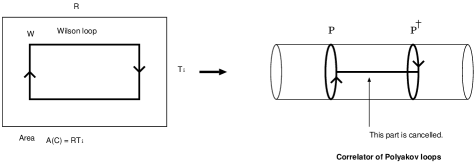
Figure 2: The correlator of Polyakov loops. The expectation value of a Wilson loop $W$ is equivalent to a correlator of the Polyakov loops $P$ and $P^{\dagger}$.

At finite temperature we must evaluate the correlator of the Polyakov loops $P({\bf x})$. It can be evaluated in the same way as the Wilson loop, due to the following relation (as shown in Fig. 2)

$$\langle P({\bf x})P^{\dagger}(0)\rangle_{\rm U(1)}=\langle W_{C}\rangle_{\rm U(1)}.$$ (17)

Furthermore, we can derive the Coulomb potential (at zero temperature) qed or Yukawa-type potential (at finite temperature) using the hard thermal loop approximation KY2 from the perturbative deformation part.

II.3 TQFT sector and PS dimensional reduction

When the gauge group is the compact $U(1)$ the TQFT sector becomes the $O(2)$ NLSM₂ through the PS dimensional reduction PS . The four-dimensional TQFT sector action

$$S_{\rm TQFT}=\delta_{\rm B}\bar{\delta}_{\rm B}\int d^{4}x\left[\frac{1}{2}\Omega_{\mu}^{2}+iC\bar{C}\right]$$ (18)

can be rewritten as the $O(2)$ NLSM₂ on the two-dimensional space,

$$S_{\rm TQFT} = \pi\int d^{2}x~{}\Omega_{\mu}^{2}(x)$$

$$= \frac{\pi}{g^{2}}\int d^{2}x\partial_{\mu}U(x)\partial_{\mu}U^{\dagger}(x),$$

$$\Omega_{\mu} \equiv \frac{i}{g}U(x)\partial_{\mu}U(x)^{\dagger},$$

where we have omitted the ghost term. When we write the gauge group element as $U(x)={\rm e}^{i\varphi(x)}$, we obtain

$$S_{\rm TQFT}=\frac{\pi}{g^{2}}\int d^{2}x\partial_{\mu}\varphi(x)\partial_{\mu}\varphi(x).$$ (19)

If the gauge group $U(1)$ is not compact, then the TQFT sector becomes the ordinary free scalar field theory on the two-dimensional space, which has no topological object. So the confining phase cannot exist. If the $U(1)$ is compact, the theory described by the action (19) is the periodic boson theory. The angle variable $\varphi(x)$ is periodic (mod $2\pi$), and so $\varphi(x)$ is a compact variable. It is well known that the compactness plays an important role in the confinement Poly . If we consider the system at finite (zero) temperature, then the dimensionally reduced theory lives on the cylinder (2-plane).

We should remark here that the compactness also leads to monopole configurations in the original gauge theory, which is assumed to play an important role in the confinement. On the other hand, the reduced theory has vortex solutions due to the compactness of $U(1)$. It is quite natural that the two configuration above are intimately connected, as suggested in Ref. qed . Therefore we can include the monopole effect from the reduced theory and obtain the physical quantity such as a string tension through this sector which includes the unphysical degrees of freedom only.

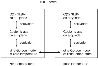
Figure 3: The TQFT sector is equivalent to the two-dimensional theory through the PS dimensional reduction. When the gauge group is the compact $U(1)$ it becomes the $O(2)$ NLSM₂. The two-dimensional space is a 2-plane (at zero temperature) or a cylinder (at finite temperature). It is well known that it is equivalent to the several model.

The $O(2)$ NLSM₂ is equivalent to the CG system as shown in Fig. 3. The partition function of the CG system is given by

$$Z_{\rm CG}=\sum_{n=0}^{\infty}\frac{\zeta^{2n}}{(n!)^{2}}\prod_{i=1}^{n}\int d^{2}x_{i}d^{2}y_{i}\exp\Bigg{(}-\frac{(2\pi)^{3}}{g^{2}}\Big{[}\sum_{i<j}[\Delta(x_{i}-x_{j})+\Delta(y_{i}-y_{j})]-\sum_{i,j}\Delta(x_{i}-y_{j})\Big{]}\Bigg{)},$$ (20)

where $\zeta\equiv\exp(-S_{\rm self})$ is the chemical potential of the CG system and can be written in terms of the self-energy part of a vortex $S_{\rm self}$. This quantity $\zeta$ does not depend on the physical temperature $T$ in the original theory. The $\Delta(x_{i}-x_{j})$ expresses the Coulomb potential on the 2-plane (at zero temperature) or on the cylinder (at finite temperature). The temperature of the CG system is defined by

$$T_{\rm CG}\equiv\frac{g^{2}}{8\pi^{3}}.$$ (21)

The linear potential between the test charged particles is induced by the effect of the vortices. The expectation value of the Wilson loop (Polyakov loops’ correlator) is obtained as follows (for details, see Ref. qed ):

$$\langle P({\bf x})P^{\dagger}(0)\rangle_{\rm U(1)} = \langle W_{C}[\Omega]\rangle\cong{\rm e}^{-\sigma A},$$ (22)

$$\sigma = \left(2\pi\frac{q}{g}\right)^{2}\zeta,$$ (23)

where $A=RT_{i}$, $R=|{\bf x}|$ and $q$ is a charge of the test particles. It is significant that the expression of the string tension (23) does not depend on the temperature explicitly, but on the behavior of the CG system. Whether the string tension remains or vanishes is determined only by the behavior of the CG system which consists of vortices. Thermal effect changes the behavior of the topological objects. The change is reflected to the linear potential. We also note that the string tension $\sigma$ is proportional to $\zeta$. The $\zeta\rightarrow 0$ limit implies that the self-energy of the vortex is infinity and we fail to include the effect of the vortex. Therefore the confining phase also vanishes in the limit $\zeta\rightarrow 0$ as is expected.

In our previous paper KY2 we have investigated the phase structure of the compact $U(1)$ gauge theory at finite temperature using the behavior of the CG system on the cylinder. The behavior of the CG system on the 2-plane is shown in Fig. 4. The behavior of the CG system on the cylinder would be analogous. We expect that the system undergoes the BKT-like phase transition. In fact, the CG system causes the BKT-like phase transition in the high-temperature region that it behaves as the one-dimensional system.

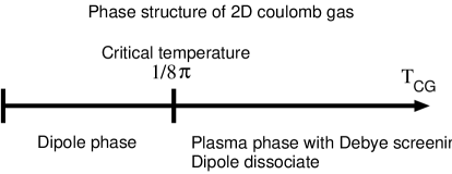
Figure 4: Two-dimensional Coulomb gas has two different phases. Over the critical temperature $T_{\rm CG}=1/8\pi$, the system is the plasma phase with Debye screening, and so the mass gap exists. Below the $T_{\rm CG}$ it is the dipole phase, in which Coulomb charges form dipoles. The system has a long-range correlation and no mass gap.

III Equivalence between SG model and CG System

The action of the SG model on the 2-plane (at zero temperature) or the cylinder (at finite temperature) is defined by

$$S_{\rm SG}=\int d^{2}x\left\{\frac{1}{2}\left(\partial_{\mu}\phi\right)^{2}-\frac{m^{4}}{\lambda}\left[\cos\left(\frac{\sqrt{\lambda}}{m}\phi\right)-1\right]\right\}.$$ (24)

The partition function is given by

$$Z_{\rm SG} = \int[d\phi]\exp\left(-S_{\rm SG}\right).$$ (25)

This can be rewritten as follows:

$$Z_{\rm SG} = {\rm e}^{-(m^{4}/\lambda)\int d^{2}x}\sum_{n=0}^{\infty}\frac{1}{n!}\left(\frac{m^{4}}{\lambda}\right)^{n}\int[d\phi]{\rm e}^{-\int d^{2}x(1/2)\left(\partial_{\mu}\phi\right)^{2}}\left[\int d^{2}x\cos\left(\frac{\sqrt{\lambda}}{m}\phi\right)\right]^{n}$$

$$= {\rm e}^{-(m^{4}/\lambda)\int d^{2}x}\sum_{n=0}^{\infty}\frac{1}{2n!}\left(\frac{m^{4}}{2\lambda}\right)^{2n}\int[d\phi]{\rm e}^{-\int d^{2}x(1/2)\left(\partial_{\mu}\phi\right)^{2}}\left[\int d^{2}x\left({\rm e}^{i(\sqrt{\lambda}/m)\phi}+{\rm e}^{-i(\sqrt{\lambda}/m)\phi}\right)\right]^{2n}$$

$$= {\rm e}^{-(m^{4}/\lambda)\int d^{2}x}\sum_{n=0}^{\infty}\frac{1}{(n!)^{2}}\left(\frac{m^{4}}{2\lambda}\right)^{2n}\int[d\phi]{\rm e}^{-\int d^{2}x(1/2)\left(\partial_{\mu}\phi\right)^{2}}\prod_{i=1}^{n}\int d^{2}x_{i}d^{2}y_{i}{\rm e}^{i(\sqrt{\lambda}/m)[\phi(x_{i})-\phi(y_{i})]}.$$

Here, we note that

$$\left\langle{\rm e}^{\int d^{2}xJ\phi}\right\rangle_{\rm SG} \equiv \int[d\phi]\exp\left[\int d^{2}x\left(-\frac{1}{2}\left(\partial_{\mu}\phi\right)^{2}+J\phi\right)\right]$$ (26)

$$= \exp\left[\int d^{2}xd^{2}yJ(x)\Delta(x-y)J(y)\right],$$

where $\Delta(x-y)$ is the massless scalar field propagator,

$$\Delta(x-y)\equiv\int\frac{d^{2}p}{(2\pi)^{2}}\frac{{\rm e}^{ip\cdot(x-y)}}{p^{2}}.$$ (27)

In particular, if we choose the external field as

$$J(x)=i\frac{\sqrt{\lambda}}{m}\sum_{i=1}^{n}q_{i}\delta(x-x_{i}),$$ (28)

then we obtain

$$\left\langle\prod_{i=1}^{n}{\rm e}^{\int d^{2}xiq_{i}\phi(x_{i})}\right\rangle_{\rm SG}=\left\{\begin{array}[]{cc}\exp\left[-\frac{\lambda}{2m^{2}}\sum_{j,k}q_{j}q_{k}\Delta(x_{j}-x_{k})\right]&{\rm for}~{}\sum_{i=1}^{n}q_{i}=0,\\ 0&{\rm for}~{}\sum_{i=1}^{n}q_{i}\neq 0.\end{array}\right.$$ (29)

If the net charge is not zero then the correlation function vanishes because of the symmetry under the transformation

$$\phi(x)\longrightarrow\phi(x)+~{}{\rm const}.$$

By the use of Eq. (26), we obtain the following expression of the partition function,

$$Z_{\rm SG}\sim\sum_{n=0}^{\infty}\frac{1}{(n!)^{2}}\left(\frac{m^{4}}{2\lambda}\right)^{2n}\prod_{i}^{n}\int d^{2}x_{i}d^{2}y_{i}\exp\Bigg{(}-\frac{\lambda}{m^{2}}\Big{(}\sum_{i<j}[\Delta(x_{i}-x_{j})+\Delta(y_{i}-y_{j})]-\sum_{i,j}\Delta(x_{i}-y_{j})\Big{)}\Bigg{)}.$$ (30)

The factor ${\rm e}^{-(m^{4}/\lambda)\int d^{2}x}$ can be ignored because of the normalization of the partition function. Thus we obtain the partition function of the neutral CG system, whose temperature is defined by

$$T_{\rm CG}=m^{2}/\lambda.$$ (31)

This is equivalent to Eq. (21). The phase transition in the SG model at the critical coupling, i.e., the Coleman transition, corresponds to the BKT phase transition in the CG system.

The equivalence holds on the cylinder (i.e., in the finite-temperature case). In this time, Eq. (27) is replaced with the propagator on the cylinder,

$$\Delta(x-y) \sim -\frac{1}{2\pi}\sum_{n=-\infty}^{+\infty}\ln\left[\mu\sqrt{(x_{0}-y_{0}-n\beta)^{2}+(x_{1}-y_{1})^{2}}\right]$$ (32)

$$= -\frac{1}{2\pi}\ln\left[\mu\beta\sqrt{\cosh\left(\frac{2\pi}{\beta}(x_{1}-y_{1})\right)-\cos\left(\frac{2\pi}{\beta}(x_{0}-y_{0})\right)}\right].$$

Here $\mu$ is the infrared cutoff and $\beta$ is the inverse of the physical temperature $T$. We remark that the SG model has the physical temperature in common with the original gauge theory. It is because the cylinder is chosen as the two-dimensional space when we use the PS dimensional reduction. If we use the complex coordinates $w=x_{1}+ix_{0},\bar{w}=x_{1}-ix_{0},w^{\prime}=y_{1}+iy_{0}$, and $\bar{w}^{\prime}=y_{1}-iy_{0}$, then Eq. (32) is rewritten as

$$\Delta(x-y)=-\frac{1}{4\pi}\ln\left|{\rm e}^{(2\pi/\beta)w}-{\rm e}^{(2\pi/\beta)w^{\prime}}\right|^{2}+\frac{1}{2\beta}{\rm Re}(w+w^{\prime})-\frac{1}{4\pi}\ln\left(\frac{1}{2}(\mu\beta)^{2}\right).$$ (33)

The propagator above involves the divergent term in the limit $\mu\rightarrow$ 0, but this is removed by the neutral condition $\sum_{i}q_{i}=0$ [see Eq. (29)].

The parameters of the CG system in the previous section, $g$ and $\zeta$, can be related to those of the SG model, mass $m$ and the coupling constant $\lambda$. This relation is given by

$$\lambda=\frac{128\pi^{6}\zeta}{g^{4}},~{}~{}~{}~{}~{}m=\frac{4\pi^{3/2}\zeta^{1/2}}{g}.$$ (34)

Recall that the string tension $\sigma\sim\zeta$ vanishes as $\sigma\rightarrow 0$ and the confining phase disappears. We should note that $\zeta\rightarrow 0$ means $m\rightarrow 0$ and $\lambda\rightarrow 0$. That is, the SG model becomes free scalar field theory in this limit. This result is consistent with the disappearance of the confining phase.

IV One-loop Effective Potential of SG Model at Finite Temperature

It is well known that the SG model at zero temperature undergoes the phase transition at certain coupling, which is called the Coleman transition Coleman . The critical coupling is $\lambda/m^{2}=8\pi$, at which the quantum SG model undergoes a phase transition from a stable vacuum to an unstable vacuum. Moreover, the existence of a phase transition due to the thermal effect has been shown in Ref. f-sine . This transition would correspond to the BKT-like transition of the CG system. Thus we can investigate the phase structure of the compact $U(1)$ gauge theory at finite temperature, at least in the region where we can investigate the SG model reliably. In particular, we can read off from Eq. (34) that the weak-coupling region of the SG model corresponds to the strong-coupling region of the gauge theory. That is, we can investigate the phase structure of the gauge theory with the strong coupling from the perturbative study of the SG model. This is the advantage of our method.

We will discuss the one-loop effective action of the two-dimensional SG model at finite temperature f-sine . The effective potential is given by

$$V_{1{\rm loop}}(\phi_{c}) = V_{\rm 0}(\phi_{c})+V_{\rm FT}(\phi_{c}),$$ (35)

$$V_{\rm 0}(\phi_{c}) \equiv \frac{m^{2}}{8\pi}\cos\left(\sqrt{\lambda}\phi_{c}/m\right)\left[1-\ln\cos\left(\sqrt{\lambda}\phi_{c}/m\right)\right],$$ (36)

$$V_{\rm FT}(\phi_{c}) \equiv \frac{1}{\pi\beta^{2}}\int^{\infty}_{0}dx\ln\left[1-\exp\left(-\sqrt{x^{2}+M^{2}(\phi_{c})\beta^{2}}\right)\right],$$ (37)

$$M^{2}(\phi_{c}) \equiv m^{2}\cos\left(\sqrt{\lambda}\phi_{c}/m\right).$$ (38)

The second equation (36) is the temperature-independent part, and the third equation (37) is the temperature-dependent part which vanishes in the zero-temperature limit $\beta\rightarrow\infty$ . Also, the minimum of the potential $\phi_{c}=0$ is still stable under one-loop quantum fluctuations at zero temperature. Taking the second derivative of Eq. (35) with respect to $\phi_{c}$ at $\phi_{c}=0$, we can evaluate a critical-line equation critical as

$$m^{2}(\beta) = m^{2}+\frac{\partial^{2}V_{\rm FT}}{\partial\phi_{c}^{2}}(\phi_{c}=0)$$ (39)

$$= m^{2}-m^{2}\frac{\bar{\lambda}}{2\pi}f(\bar{\beta})=0,$$

where $\bar{\lambda}\equiv\lambda/m^{2}$, $\bar{\beta}\equiv\beta m$, and $f(\bar{\beta})$ is defined by

$$f(\bar{\beta})\equiv\int^{\infty}_{0}dx\frac{1}{\sqrt{\bar{\beta}^{2}+x^{2}}\left[\exp\left(\sqrt{\bar{\beta}^{2}+x^{2}}\right)-1\right]}.$$ (40)

That is, the critical-line equation is given by

$$1-\frac{\bar{\lambda}}{2\pi}f(\bar{\beta})=0.$$ (41)

Note that the parameters of the SG model can be replaced with the ones of the compact $U(1)$ gauge theory using the relation (34). As the result, we obtain the relation

$$\bar{\beta}=\frac{4\pi^{3/2}\zeta^{1/2}}{gT},~{}~{}\bar{\lambda}=\frac{8\pi^{3}}{g^{2}}.$$ (42)

Thus the critical-line equation can be rewritten as follows,

$$1-\frac{4\pi^{2}}{g^{2}}f\left(\frac{4\pi^{3/2}\zeta^{1/2}}{gT}\right)=0.$$ (43)

The numerical solutions of this equation at various fixed values of $\zeta$ are shown in Fig. 5.

Figure 5: The phase structure of the compact $U(1)$ gauge theory obtained by the one-loop effective potential calculation in the SG model. The critical-line Eq. (43) can be numerically solved. The asymptotic line Eq. (45) is also drawn with the dashed line. The above graph shows that the confining phase vanishes in $\zeta\rightarrow 0$ limit. However, the result in the small $g$ region is not valid. It is because the small $g$ means the large $\lambda$ and the one-loop approximation in the SG model is not reliable.

In particular, we can derive the simple relation between $\lambda$ and $T$ in the weak-coupling and high-temperature limit of Eq. (41). The critical temperature $T_{c}$ is given by

$$T_{c}=\frac{4m^{3}}{\lambda}.$$ (44)

Equations.(34) and (44) lead to

$$T_{c}=\frac{2\zeta^{1/2}}{\pi^{3/2}}g.$$ (45)

Equation (45) is drawn as the dashed line in Fig. 5. Note again that the weak-coupling and high-temperature region in the SG model corresponds to the strong-coupling and high-temperature region in the compact $U(1)$ gauge theory. The compact gauge theory is related to the SG model by a kind of S-duality in our scenario. Thus we can reliably investigate the strong-coupling region of the gauge theory since the one-loop effective potential is appropriate in the weak-coupling region.

In conclusion, we have obtained that the critical temperature is proportional to the coupling constant of the compact $U(1)$ gauge theory in the strong-coupling and high-temperature region. This result is in good agreement with the prediction in Ref. SV . In the $\zeta\rightarrow 0$ limit the gradient in Eq. (45) goes to zero. This fact implies that the confining phase disappears.

Comment on the effective potential calculation. Our discussion in this section is closely analogous to Ref. HT in which the critical temperature has been estimated by the calculation of the one-loop effective potential in the TQFT sector. In the above discussion we have calculated the one-loop effective potential in the SG model. If we naively calculate the effective potential in the $O(2)$ NLSM₂ then we cannot obtain the phase structure HT ; KY . Note that the $O(2)$ NLSM₂ is equivalent to the SG model when we consider vortex solutions. If we calculate the effective potential in the $O(2)$ NLSM₂ we cannot include the effect of the vortex solution. However, once we go from the $O(2)$ NLSM₂ to the SG model, we can include the effect of the vortex solution in terms of the cosine-type potential. Therefore the phase structure that we have obtained in the SG model is not equivalent to the result in the $O(2)$ NLSM₂. Moreover, the SG model is a massive theory and the Coleman-Mermin-Wagner theorem CMW is not an obstacle.

Figure 6: Phase structure of the compact $U(1)$ gauge theory predicted in Ref. SV . In the above discussion using the one-loop effective potential of the SG model we could study the region enclosed by the dashed line, in which we can especially obtain the critical-line equation. Moreover, we might investigate the region enclosed by the solid line. It is well known that this region is neatly described by the Gaussian effective potential (GEP), which is a nonperturbative method and should include the physics beyond the one-loop level.

V Conclusion and Discussion

We have discussed the phase structure of the compact $U(1)$ gauge theory at finite temperature by using a deformation of the topological model. The compactness of the gauge group leads to a confining phase. In the case of zero temperature, the phase transition of the gauge theory at certain coupling can be described by the Coleman transition in the SG model. In the finite temperature case we could investigate the phase structure at sufficiently high-temperature and very strong-coupling region by analyzing the one-loop effective potential of the SG model. We could consider the enclosed region by the dashed line in Fig. 6. In this paper we have used the one-loop effective potential, but we can also use the Gaussian effective potential (GEP) st , which is known as the nonperturbative method. For the SG model at zero temperature this is given by the following expression:

$$V_{\rm GEP}=m^{2}\frac{1-\bar{\lambda}/8\pi}{\bar{\lambda}}\left[1-(\cos\sqrt{\bar{\lambda}}\phi)^{1/(1-\bar{\lambda}/8\pi)}\right],$$ (46)

where $\bar{\lambda}=\lambda/m^{2}$. That is, as the coupling constant of the SG model $\bar{\lambda}\rightarrow 8\pi$ the GEP becomes a straight line continuously. If $\bar{\lambda}$ exceeds $\bar{\lambda}_{c}=8\pi$, which is the transition point of the Coleman transition, then the GEP has the maximum and the system has no ground state. The GEP can describe the Coleman transition at zero temperature I ; gep-sg , which cannot be described by the one-loop effective potential. Since the GEP does not depend on the perturbation theory it might be appropriate to investigate the phase structure at weak-coupling and low-temperature region in the gauge theory (i.e., the strong-coupling and low-temperature region in the SG model) which corresponds to the enclosed region by the solid line in Fig. 6. This work is very interesting and will be discussed in another place KY5 .

We should comment on the well-known results in the compact Abelian lattice gauge theory. This theory at zero temperature experiences the phase transition of the weak first or strong second order. Unfortunately, our results suggest that at high temperatures the phase transition is of the BKT type, and do not seem to correspond to the lattice results. Our formalism deeply depends on the BKT phase transition, and so it seems difficult to predict the order of the transition obtained in the lattice gauge theory.

It is also attractive to approach the phase structure from the viewpoint of the massive Thirring model steer .