Thermal Fluctuations of Induced Fermion Number

Abstract

We analyze the phemomenon of induced fermion number at finite temperature. At finite temperature, the induced fermion number $\langle N\rangle$ is a thermal expectation value, and we compute the finite temperature fluctuations, $(\Delta N)^{2}=\langle N^{2}\rangle-\langle N\rangle^{2}$. While the zero temperature induced fermion number is topological and is a sharp observable, the finite temperature induced fermion number is generically nontopological, and is not a sharp observable. The fluctuations are due to the mixing of states inherent in any finite temperature expectation value. We analyze in detail two different cases in $1+1$ dimensional field theory: fermions in a kink background, and fermions in a chiral sigma model background. At zero temperature the induced fermion numbers for these two cases are very similar, but at finite temperature they are very different. The sigma model case is generic and the induced fermion number is nontopological, but the kink case is special and the fermion number is topological, even at finite temperature. There is a simple physical interpretation of all these results in terms of the spectrum of the fermions in the relevant background, and many of the results generalize to higher dimensional models.

I Introduction

The phenomenon of induced fermion number arises due to the interaction of fermions with nontrivial topological backgrounds (e.g., solitons, vortices, monopoles, skyrmions), and has many applications ranging from polymer physics to particle physics jr ; gw ; jackiw2 ; niemi ; polymer ; roman . The original fractional fermion number result of Jackiw and Rebbi jr provides the physical explanation of the existence of spinless charged excitations in polymers polymer ; roman ; ssh ; rice ; js . The adiabatic analysis of Goldstone and Wilczek gw in systems without conjugation symmetry has important implications for model field theories in particle physics, such as bag models bag , electroweak theories eric , and chiral sigma models diakonov . At zero temperature, the induced fermion number is a topological quantity, and is related to the spectral asymmetry of the relevant Dirac operator, which counts the difference between the number of positive and negative energy states in the fermion spectrum jackiw2 ; niemi ; roman ; rich ; wilczek ; yamagishi ; boy ; mike ; manu ; jaffe2 . Mathematical results, such as index theorems manu ; niemi and Levinson’s theorem yamagishi ; boy ; mike ; jaffe2 , imply that the zero temperature induced fermion number is determined by the asymptotic topological properties of the background fields. This topological character of the induced fermion number is a key feature of its application in certain model field theories bag ; eric ; diakonov .

At finite temperature, the situation is less clear-cut. In several examples, namely the $1+1$ dimensional chiral kink background ns ; soni ; keil and the $3+1$ dimensional Dirac cp ; monopole and ’t Hooft-Polyakov monopole goldhaber backgrounds, the finite temperature induced fermion number has been shown to be temperature dependent, but still topological in the sense that the only dependence on the background field is through its asymptotic properties. However, it has recently been demonstrated ad that the finite temperature induced fermion number need not be topological. Explicitly, in a $1+1$ dimensional chiral sigma model, the finite temperature induced fermion number depends on the detailed structure of the background, not just its asymptotic behavior. This result corrects several previous analyses midorikawa ; nnp that had claimed that the finite temperature fermion number was in general a topological quantity (at zero chemical potential). In ad , an explicit calculation showed that the finite temperature fermion number can be nontopological, and a simple physical explanation was given for the origin of the nontopological fermion number as the plasma response of the fermions to the inhomogeneous background. A possible source of confusion here is that while the kink and sigma model cases are very similar at zero temperature, it is not widely appreciated that at finite temperature they are very different. In this paper we present more details of this analysis, and we present a general argument that the finite temperature fermion number naturally separates into a temperature-independent topological piece that corresponds to vacuum polarization effects, and a temperature-dependent piece that is generically nontopological, and which corresponds to the thermal occupation of excited states of the fermion Fock space. While this temperature-dependent piece is generically nontopological, for certain particular backgrounds (such as, for example, the kink background) the fermion spectrum has a special symmetry, which has the consequence that the temperature-dependent corrections are in fact themselves topological.

Another motivation for our work concerns the nature of the induced fermion number as a sharp quantum observable. At zero temperature it has been shown that the fractional induced fermion number is indeed a sharp observable kivelson ; bell ; jackiw ; frishman ; charge . In this paper we address this question at finite temperature by computing the rms fluctuations, $(\Delta N)^{2}=\langle N^{2}\rangle-\langle N\rangle^{2}$, in the induced fermion number $\langle N\rangle$. We compute the finite temperature fluctuation in two different cases, and show that $\Delta N$ is generally nonzero (and nontopological) at finite temperature, but that $\Delta N$ vanishes at zero temperature. This indicates that $N$ is not a sharp quantum observable at nonzero temperature. The nonvanishing fluctuations are due to the mixing of Fock states inherent in the thermal expectation value. It is interesting to note that another example of non-sharp fractional fermion number (but not in the context of temperature dependence) has been discussed recently in the context of liquid helium bubbles helium .

Our analysis of finite temperature fermion number has also been motivated by the realization over recent years that certain types of anomalies in zero temperature field theory become much more subtle at finite temperature. For example, Pisarski et al have explained pisarski why finite temperature anomalous $\pi^{0}$ decay amplitudes are temperature dependent even though the chiral anomaly (a topological object that is known to be related to the anomalous $\pi^{0}$ decay amplitude at $T=0$) is known to be temperature independent. These and related issues have also been explored in $1+1$ dimensions gelis . And in odd spacetime dimensions, it has recently been realized dll ; deser ; fosco ; lh that while the topological Chern-Simons term is the only parity-violating term that can be induced in the $T=0$ effective action, at finite temperature there are infinitely many other parity-violating terms, all of which vanish identically at zero temperature, but all of which are crucial, for example, for understanding how it is possible to maintain large gauge invariance at finite temperature. These results have led us to reconsider the related general question of induced fermion number at finite temperature.

In Section II we define what is meant by finite temperature induced fermion number, and indicate how it can be computed. In Section III we give more details of the derivations and results of ad for the finite temperature induced fermion number $\langle N\rangle$ for a kink background and for a sigma model background in $1+1$ dimensional field theory. Section IV presents the computation of the finite temperature fluctuations, $(\Delta N)^{2}=\langle N^{2}\rangle-\langle N\rangle^{2}$, in the induced fermion number for the kink case and for the sigma model case. In Section V we give a simple physical interpretation of all these results in terms of the thermal occupation of the available levels in the Dirac spectrum, according to Fermi-Dirac statistics. We conclude in Section VI and give some general comments regarding the extension of our results to higher dimensional theories.

II Finite Temperature Induced Fermion Number

Consider an abelian model in $1+1$ dimensions with fermions interacting via scalar and pseudoscalar couplings to two bosonic fields $\phi_{1}$ and $\phi_{2}$. For the purposes of this paper, $\phi_{1}$ and $\phi_{2}$ will be considered as static classical background fields. The Lagrangian is

$${\cal L}=i\,\bar{\psi}{\partial\hskip-6.0pt/}\,\psi-\bar{\psi}\left(\phi_{1}+i\,\gamma_{5}\,\phi_{2}\right)\psi$$ (1)

We will concentrate on two important physical cases:

Figure 1: In the kink case (2), the kink function $\phi_{2}(x)$ has the form shown in the solid line, with asymptotic values $\pm\hat{\phi_{2}}$. The corresponding angular field defined in (4), $\theta(x)={\rm arctan}(\frac{\phi_{2}(x)}{m})$, also has a kink-like shape, as shown in the dashed line, with asymptotic values $\-pm\hat{\theta}$, where $\hat{\theta}={\rm arctan}(\frac{\hat{\phi_{2}}}{m})$. Note that in the kink case, the allowed values of $\hat{\theta}$ lie in the first branch $[-\frac{\pi}{2},\frac{\pi}{2}]$ of the arctan function.

Figure 2: In the sigma model case (3), it is the angular field $\theta(x)$ defined in (4) that has a kink-like shape, with asymptotic values $\pm\hat{\theta}$.

(i) kink case jr : $\phi_{1}$ is constant, but $\phi_{2}=\phi_{2}(x)$ has a kink-like shape, as shown in Fig. 1:

$$\phi_{1}=m,\qquad{\rm and}\quad\phi_{2}={\rm kink},\,\,{\rm with}\quad\phi_{2}(\pm\infty)=\pm\hat{\phi_{2}}$$ (2)

(ii) sigma model case gw : $\phi_{1}$ and $\phi_{2}$ are both x-dependent, but are constrained to the “chiral circle”:

$$\phi_{1}^{2}+\phi_{2}^{2}=m^{2}$$ (3)

In each case, we define a corresponding angular field

$$\theta(x)\equiv{\rm arctan}\,\left(\frac{\phi_{2}(x)}{\phi_{1}(x)}\right)$$ (4)

In the kink case (2), the angular field $\theta(x)={\rm arctan}\,(\frac{\phi_{2}(x)}{m})$ also has a kink-like shape, as shown in Fig. 1. In the sigma model case (3), the angular field $\theta(x)$ has the interpretation of a local chiral angle, since the chiral constraint (3) allows us to write $\phi_{1}=m\cos\theta$ and $\phi_{2}=m\sin\theta$, so that the interaction term in the Lagrangian (1) is

$$m\bar{\psi}\left(\cos\theta+i\gamma_{5}\sin\theta\right)\psi=m\bar{\psi}\,e^{i\gamma_{5}\theta}\,\psi$$ (5)

In this sigma model case, it is the angular field $\theta(x)$ that has a kink-like shape, as shown in Fig. 2.

The second-quantized fermion number operator is defined bjorken as $N=\frac{1}{2}[\Psi^{\dagger},\Psi]$. The fermion field operator $\Psi$ may be expanded in a complete set of eigenstates of the Dirac Hamiltonian $H$ for fermions in the presence of the background fields $\phi_{1}$ and $\phi_{2}$. The Dirac Hamiltonian corresponding to the Lagrangian (1) is

$$H = -i\gamma^{0}\gamma^{1}\nabla+\gamma^{0}\phi_{1}(x)+i\gamma^{0}\gamma_{5}\phi_{2}(x)$$ (6)

$$= \left(\matrix{\phi_{1}&-i\nabla-i\phi_{2}\cr-i\nabla+\phi_{2}&-\phi_{1}}\right)$$

where $\nabla\equiv\frac{d}{dx}$, and we have chosen to work with the Dirac matrices: $\gamma^{0}=\sigma_{3}$, $\gamma^{1}=i\sigma_{2}$, and $\gamma^{5}=-\sigma_{1}$. The presence of the background fields modifies the fermion spectrum from the free case. All necessary information about the fermion spectrum can be encoded in terms of the spectral function $\sigma(E)$ of the Dirac Hamiltonian in (6):

$$\sigma(E)=\frac{1}{\pi}\,{\cal I}m\,{\rm Tr}\left(\frac{1}{H-E-i\epsilon}\right)$$ (7)

The zero temperature vacuum expectation value, $\langle 0|N|0\rangle\equiv\langle N\rangle_{0}$, of the number operator can be expressed as jackiw2 ; niemi

$$\langle N\rangle_{0}=-\frac{1}{2}\int_{-\infty}^{\infty}dE\,\sigma(E)\,{\rm sign}(E)$$ (8)

where the subscript $0$ refers to zero temperature. Thus, $\langle N\rangle_{0}$ is expressed in terms of the spectral asymmetry of the Dirac operator, which counts the number of positive energy states minus the number of negative energy states.

At zero temperature, in both the kink case (2) and the sigma model case (3), the induced fermion number (8) is given by the simple expression gw :

$$\langle N\rangle_{0}=\frac{1}{2\pi}\int_{-\infty}^{\infty}dx\,\theta^{\prime}=\frac{1}{\pi}\,\hat{\theta}$$ (9)

where $\theta(x)$ is the angular field defined in (4), and $\hat{\theta}$ is the asymptotic value of $\theta(x)$ at $x=+\infty$. The zero temperature fermion number $\langle N\rangle_{0}$ is topological in the sense that it depends only on the asymptotic value $\hat{\theta}$, and not on the detailed shape of $\theta(x)$. The original conjugation symmetric case of Jackiw and Rebbi jr is obtained by taking $m\to 0$ in the kink case (2), in which case $\langle N\rangle_{0}\to\pm\frac{1}{2}$. In Section IV we will show that the zero temperature expectation value (8) is in fact also a sharp eigenvalue.

At nonzero temperature, the induced fermion number is a thermal expectation value

$$\langle N\rangle_{\rm T} = \frac{{\rm Tr}\,(N\,e^{-\beta H})}{{\rm Tr}\,(e^{-\beta H})}$$ (10)

$$= -\frac{1}{2}\int_{-\infty}^{\infty}dE\,\sigma(E)\,\tanh\left(\frac{\beta E}{2}\right)$$

where $\beta=\frac{1}{T}$ is the inverse temperature. Note that as $T\to 0$, which means $\beta\to\infty$, only the vacuum state survives in the trace, and $\langle N\rangle_{\rm T}$ reduces to the vacuum expectation value $\langle N\rangle_{0}$. Correspondingly, $\tanh(\frac{\beta E}{2})\to{\rm sign}(E)$, so that the integral expression in (10) reduces smoothly to the spectral asymmetry expression in (8). In fact, the finite temperature expression (10) provides a physically natural, and computationally simple, regularization of the spectral asymmetry (8). In Section IV we will show that at nonzero temperature the fermion number expectation value (10) is not a sharp eigenvalue.

To compute $\langle N\rangle_{0}$ or $\langle N\rangle_{\rm T}$, one needs information about the spectral function $\sigma(E)$. We stress, of course, that $\sigma(E)$ has nothing to do with the temperature; it simply describes the spectrum of the fermions in the presence of the static background fields $\phi_{1}$ and $\phi_{2}$. One convenient way to proceed is to use the expression (7) for the spectral function to write (10) as a contour integral in the complex energy plane:

$$\langle N\rangle_{\rm T}=-\frac{1}{2}\int_{\cal C}\,\frac{dz}{2\pi i}\,{\rm tr}\left(\frac{1}{H-z}\right){\rm tanh}\left(\frac{\beta z}{2}\right)$$ (11)

Here ${\rm tr}(\frac{1}{H-z})$ is the resolvent of the Dirac Hamiltonian $H$, and the contour ${\cal C}$ is $(-\infty+i\epsilon,+\infty+i\epsilon)$ and $(+\infty-i\epsilon,-\infty-i\epsilon)$, as shown in Fig. 3. Since $H$ has a real spectrum, we can evaluate the contour integral (11) in two alternative ways. First, we can deform the contour around the simple poles of the $\tanh(\frac{\beta z}{2})$ function, which occur along the imaginary axis at the Matsubara modes: $z_{n}=(2n+1)i\pi T$, for $n\in{\bf Z}$. This leads to an expression for $\langle N\rangle_{\rm T}$ as an infinite sum. Alternatively, we can deform the $z$ contour around the poles and cuts of the spectrum of $H$, which lie on the real axis. This leads to an integral representation for $\langle N\rangle_{\rm T}$, which is just the Sommerfeld-Watson transform of the infinite sum expression. We will see examples of these equivalent forms below.

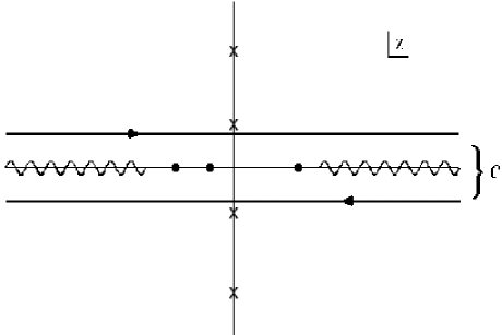
Figure 3: The contour ${\cal C}$ in the complex energy plane used in the evaluation of the contour integral in (11). The spectrum of the Dirac Hamiltonian lies on the real axis and is indicated schematically by the continuum cuts and some possible bound states in the gap. The crosses on the imaginary axis depict the simple poles, $z_{n}=(2n+1)\pi iT$, of $\tanh(\frac{\beta z}{2})$.

III Results for Finite Temperature Induced Fermion Number

Since $\tanh(\frac{\beta E}{2})$ is an odd function of $E$, it follows from (10) that to compute $\langle N\rangle_{\rm T}$ we only need the odd part, $\sigma_{\rm odd}(E)=\frac{1}{2}[\sigma(E)-\sigma(-E)]$, of the spectral function:

$$\langle N\rangle_{\rm T}=-\int_{0}^{\infty}dE\,\sigma_{\rm odd}(E)\,\tanh\left(\frac{\beta E}{2}\right)$$ (12)

Correspondingly, we only need to know the even part of the resolvent:

$$\langle N\rangle_{\rm T}=-\frac{1}{2}\int_{\cal C}\,\frac{dz}{2\pi i}\,\left[{\rm tr}\left(\frac{1}{H-z}\right)\right]_{\rm even}{\rm tanh}\left(\frac{\beta z}{2}\right)$$ (13)

This fact simplifies the calculations considerably, and has important physical consequences, as will be discussed in Section V.

III.1 Finite T Fermion Number in the Kink Case

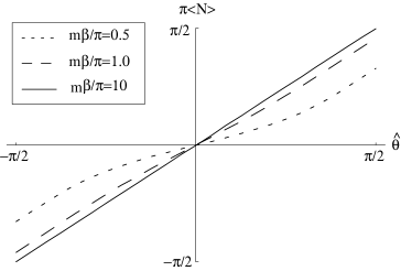
Figure 4: Plots of ($\pi$ times) the finite temperature induced fermion number $\langle N\rangle$, given in (17) and (18), for the kink case. The plots show the dependence of $\pi\langle N\rangle$ on the asymptotic value $\hat{\theta}={\rm arctan}(\frac{\hat{\phi_{2}}}{m})$, for various values of the temperature, as indicated. Note that for low temperature (large $\beta$), $\langle N\rangle$ smoothly approaches the zero temperature result $\langle N\rangle=\hat{\theta}/\pi$ in (9).

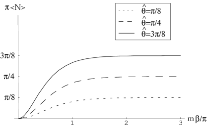
Figure 5: Plots of ($\pi$ times) the finite temperature induced fermion number $\langle N\rangle$, given in (17) and (18), for the kink case. The plots show the dependence of $\pi\langle N\rangle$ on the inverse temperature $\frac{m\beta}{\pi}$, for various values of the asymptotic value $\hat{\theta}$, as indicated. Note that for low temperature (large $\beta$), $\langle N\rangle$ quickly saturates to the zero temperature value $\pi\langle N\rangle=\hat{\theta}$. Also note that $\langle N\rangle$ vanishes as $T\to\infty$.

For the kink case (2) we can use the remarkable result (a special case of the Callias index theorem callias ) that the even part of the resolvent (and hence the odd part of the spectral function) can be computed exactly for any kink $\phi_{2}(x)$:

$$\left[{\rm tr}\left(\frac{1}{H-z}\right)\right]_{\rm even}={-m\hat{\phi}_{2}\over(m^{2}-z^{2})\,\sqrt{m^{2}+\hat{\phi}_{2}^{2}-z^{2}}}$$ (14)

Notice that this only depends on the kink $\phi_{2}(x)$ through its asymptotic value $\hat{\phi}_{2}$; it is otherwise independent of the details of the shape of the kink.

To motivate this fact, we can express the Dirac resolvent as ${\rm tr}\left(\frac{1}{H-z}\right)={\rm tr}\left((H+z)\frac{1}{H^{2}-z^{2}}\right)$, and note that, for the kink case, $H^{2}$ takes the simple diagonal form

$$H^{2}=\left(\matrix{-\nabla^{2}+m^{2}+\phi_{2}^{2}+\phi_{2}^{\prime}&0\cr 0&-\nabla^{2}+m^{2}+\phi_{2}^{2}-\phi_{2}^{\prime}}\right)$$ (15)

Thus,

$$\left[{\rm tr}\left(\frac{1}{H-z}\right)\right]_{\rm even} = {\rm tr}\left({m\over-\nabla^{2}+\phi_{2}^{2}+\phi_{2}^{\prime}+m^{2}-z^{2}}\right)-{\rm tr}\left({m\over-\nabla^{2}+\phi_{2}^{2}-\phi_{2}^{\prime}+m^{2}-z^{2}}\right)$$ (16)

That is, we can express the even part of the Dirac resolvent as the difference of two Schrödinger resolvents, with the corresponding Schrödinger potentials, $V_{\pm}=\phi_{2}^{2}\pm\phi_{2}^{\prime}$, being isospectral. This isospectrality property is the key ingredient for proving (14).

Given the result (14), the induced fermion number (13) for the kink case (2) is ad

$$\langle N\rangle_{\rm T}=\frac{2}{\pi}\,\left(\frac{m\beta}{\pi}\right)^{2}{\rm sin}\hat{\theta}\,\sum_{n=0}^{\infty}{1\over\left((2n+1)^{2}+(\frac{m\beta}{\pi})^{2}\right)\sqrt{(2n+1)^{2}\cos^{2}\hat{\theta}+(\frac{m\beta}{\pi})^{2}}}$$ (17)

where we recall that $\hat{\theta}\equiv{\rm arctan}(\frac{\hat{\phi_{2}}}{m})$, and we can restrict our attention to $-\frac{\pi}{2}\leq\hat{\theta}\leq\frac{\pi}{2}$. As an alternative to the summation expression in (17), we can write $\langle N\rangle_{\rm T}$ as an integral representation:

$$\langle N\rangle_{\rm T}=\frac{1}{2}\,{\rm sign}(\hat{\theta})\,\tanh(\frac{m\beta}{2})-\frac{\sin\hat{\theta}\,\cos\hat{\theta}}{\pi}\int_{1}^{\infty}du\,\frac{\tanh(\frac{m\beta}{2}\sec\hat{\theta}\,u)}{\sqrt{u^{2}-1}\,(u^{2}-\cos^{2}\hat{\theta})}$$ (18)

The kink case induced fermion number $\langle N\rangle_{\rm T}$ is plotted in Fig. 4 as a function of $\hat{\theta}$ for various values of the temperature, and in Fig. 5 as a function of $\frac{m\beta}{\pi}$, for various values of $\hat{\theta}$. The integral form (18) makes the zero temperature limit clear : using the integral

$$\int_{1}^{\infty}du\,\frac{1}{\sqrt{u^{2}-1}\,(u^{2}-\cos^{2}\hat{\theta})}=\frac{\frac{\pi}{2}-|\hat{\theta}|}{|\sin\hat{\theta}|\cos\hat{\theta}}$$ (19)

it follows that the leading correction to $\langle N\rangle_{0}$ at low temperature is exponentially small :

$$\langle N\rangle_{\rm T}\,\sim\,\frac{\hat{\theta}}{\pi}-{\rm sign}(\hat{\theta})\,e^{-m\beta}+\dots\quad,\quad\beta\to\infty$$ (20)

Thus $\langle N\rangle_{\rm T}$ reduces smoothly to the zero temperature expression (9). This can be seen clearly in Figs. 4 and 5. But at finite temperature, the expressions (17) and (18) for the induced fermion number are much more complicated than the $T=0$ result (9). Nevertheless, $\langle N\rangle_{\rm T}$ in (17) and (18) is still topological in the sense that it only depends on the kink background through the asymptotic value $\hat{\theta}={\rm arctan}(\hat{\phi}_{2}/m)$. Other details of the kink shape do not matter. We will see in the next subsection that this is not true in the sigma model case (3). It is also interesting to note that the angular nature of the parameter $\hat{\theta}$ is clearly manifest in the finite temperature expressions (17) and (18), while it is not as obvious from looking at the zero temperature expression (9). A similar observation applies for the finite temperature induced fermion number in $3+1$ dimensions for fermions in the presence of a Dirac monopole cp ; monopole , and for fermions in the presence of a static ‘t Hooft-Polyakov monopole goldhaber ; ad .

III.2 Finite T Fermion Number in the Sigma Model Case

In the sigma model case (3), the Callias index theorem result (14) for the even part of the resolvent does not apply. There is no general expression for the even part of the resolvent. This is because in the sigma model case

$$H^{2}=\left(\matrix{-\nabla^{2}+m^{2}&0\cr 0&-\nabla^{2}+m^{2}}\right)+m\,\theta^{\prime}\,\left(\matrix{\cos\theta&-i\sin\theta\cr i\sin\theta&-\cos\theta}\right)$$ (21)

which is clearly not of the diagonal isospectral form in (15). Thus, another approach is needed to evaluate the resolvent. In ad , the derivative expansion was used to evaluate the even part of the resolvent as an expansion in powers of $\theta^{\prime}$ and its derivatives. The derivative expansion ian ; ad assumes that $\theta^{\prime}\ll m$ : the spatial derivatives of the background fields are assumed small compared to the fermion mass scale $m$. In other words, the background chiral field $\theta(x)$ is assumed to be slowly varying on the scale of the fermion Compton wavelength. To next-to-leading order in the derivative expansion for the sigma model case, one finds ad

$$\left[{\rm tr}\left(\frac{1}{H-z}\right)\right]_{\rm even}=-\frac{m^{2}}{2(m^{2}-z^{2})^{3/2}}\int dx\,\theta^{\prime} - \frac{m^{2}}{8(m^{2}-z^{2})^{5/2}}\int dx\,\theta^{\prime\prime\prime}-\frac{m^{2}(4z^{2}+m^{2})}{16(m^{2}-z^{2})^{7/2}}\int dx\,(\theta^{\prime})^{3}+\dots$$ (22)

where the dots refer to terms involving five or more derivatives. The middle term vanishes since $\int dx\,\theta^{\prime\prime\prime}=0$ if $\theta(x)$ has a kink-like shape. Inserting this approximate expression into (13) we obtain:

$$\langle N\rangle_{\rm T}=\frac{1}{\pi}\left(\frac{m\beta}{\pi}\right)^{2}\left\{\sum_{n=0}^{\infty}\frac{1}{[(2n+1)^{2}+(\frac{m\beta}{\pi})^{2}]^{3/2}}\,\int dx\,\theta^{\prime}+\frac{\beta^{2}}{8\pi^{2}}\,\sum_{n=0}^{\infty}{[-4(2n+1)^{2}+(\frac{m\beta}{\pi})^{2}]\over[(2n+1)^{2}+(\frac{m\beta}{\pi})^{2}]^{7/2}}\,\int dx\,(\theta^{\prime})^{3}+\dots\right\}$$ (23)

The first term is topological and reduces smoothly to the zero temperature result (9) as $T\to 0$. The second term involves $\int dx\,(\theta^{\prime})^{3}$, which is clearly not topological : it depends on the actual shape of the chiral field $\theta(x)$, not just its asymptotic value $\hat{\theta}$. This is still consistent (to this order) with the topological nature of the zero temperature induced fermion number (9), because the energy trace prefactor multiplying the $\int dx\,(\theta^{\prime})^{3}$ term in (23) vanishes at $T=0$.

Higher orders in the derivative expansion (22) can be developed systematically, although it becomes somewhat tedious to enumerate all the different terms at high orders. However, a remarkable simplification occurs ad in the low temperature limit where $T\ll m$. The leading low $T$ terms at each order of the derivative expansion have the simple form :

$$\langle N\rangle^{(2l-1)}_{\rm T}\sim\delta_{l,1}\,\frac{1}{2\pi}\int dx\,\theta^{\prime}-\sqrt{\frac{2mT}{\pi}}\,e^{-m/T}\,\frac{1}{(2l-1)!}\,\int dx\,\left(\frac{\theta^{\prime}}{2T}\right)^{2l-1}+\dots$$ (24)

Thus, in the low temperature limit, we can resum the entire derivative expansion, to obtain the induced fermion number in the sigma model case (3) :

$$\langle N\rangle_{\rm T}=\frac{1}{2\pi}\int_{-\infty}^{\infty}dx\,\theta^{\prime}-\sqrt{\frac{2mT}{\pi}}\,e^{-m/T}\,\int_{-\infty}^{\infty}dx\,{\rm sinh}\left(\frac{\theta^{\prime}}{2T}\right)+\dots$$ (25)

where the dots refer to power-law subleading terms for $T\ll m$.

Note that $\langle N\rangle_{\rm T}$ in (25) naturally splits into a temperature independent topological term, and a temperature dependent nontopological term. This has a simple physical explanation ad . First, observe that the chiral sigma model background acts like a spatially inhomogeneous electric field rich ; wilczek , as can be seen by making a local chiral rotation: $\psi\to\tilde{\psi}=e^{i\theta\gamma_{5}/2}\psi$. In terms of these chirally rotated fields the Lagrangian (1), with interaction (5), becomes

$${\cal L}=i\bar{\tilde{\psi}}{\partial\hskip-6.0pt/}\tilde{\psi}-m\bar{\tilde{\psi}}\tilde{\psi}-\bar{\tilde{\psi}}\,\gamma^{0}\,\frac{\theta^{\prime}}{2}\,\tilde{\psi}$$ (26)

Thus, the chiral field $\theta(x)$ acts as an inhomogeneous scalar potential $A_{0}(x)=\frac{1}{2}\theta^{\prime}(x)$, leading to an inhomogeneous electric field

$$E(x)=-\frac{1}{2}\,\theta^{\prime\prime}(x)$$ (27)

This electric field acts on the Dirac sea to polarize the vacuum by aligning the virtual vacuum dipoles of the Dirac sea, producing a localized build-up of charge near the kink center. This leads to the first, topological, term in (25), which is just the familiar zero temperature result rich ; wilczek . It is temperature independent as the short-lived virtual electron-positron dipoles of the Dirac sea do not come to thermal equilibrium. The second, nontopological, term in (25) arises as the response of the real charges in the thermal plasma to the spatially inhomogeneous electric field ad . The linear response lebellac of the plasma at low temperature to such an electric field yields an induced fermion number density

$$\rho(x)=\int\frac{dk}{2\pi}\,f(x,k)$$ (28)

where $f(x,k)=f_{+}(x,k)-f_{-}(x,k)$ is expressed in terms of the particle and antiparticle Fermi densities. In the derivative expansion limit, the leading effect of the background is that of an inhomogeneous chemical potential $\mu(x)=-\frac{1}{2}\,\theta^{\prime}(x)$. Thus, in this limit, the local Fermi particle and antiparticle distribution functions are

$$f_{\pm}(x,k)={1\over e^{\beta(\sqrt{k^{2}+m^{2}}\mp\mu(x))}+1}$$ (29)

The resummed derivative expansion expression (25) was obtained in the low temperature ($T\ll m$) limit. In this limit, we can write

$$f_{+}(x,k)-f_{-}(x,k) \approx e^{-\beta\sqrt{k^{2}+m^{2}}}\left(e^{\beta\mu(x)}-e^{-\beta\mu(x)}\right)$$ (30)

$$= -2e^{-\beta\sqrt{k^{2}+m^{2}}}\,\sinh\left(\frac{\theta^{\prime}}{2T}\right)$$

Note that $f_{+}-f_{-}$ vanishes smoothly as $T\to 0$ in the derivative expansion regime, because $\theta^{\prime}\ll m$. For low temperature, the leading behavior of the k integral in (28) is

$$\int_{-\infty}^{\infty}\frac{dk}{2\pi}\,e^{-\beta\sqrt{k^{2}+m^{2}}}\sim\,\sqrt{\frac{mT}{2\pi}}\,e^{-\beta m}+\dots\qquad,\qquad T\to 0$$ (31)

Therefore, the plasma linear response contribution (28) to the induced fermion number gives precisely the second, nontopological, term in the formula (25) which was obtained by resumming the derivative expansion at low temperature.

IV Thermal Fluctuations of Induced Fermion Number

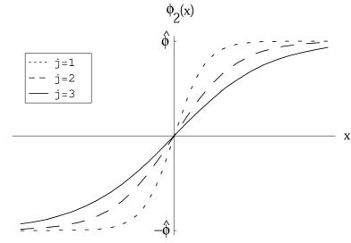
Figure 6: Plots of the special kink backgrounds in (34) for various values of j, illustrating the interpretation of the parameter j as a scale parameter that characterizes a nontopological aspect of these kinks.

We now turn to the fluctuation, $(\Delta N)^{2}_{\rm T}=\langle N^{2}\rangle_{\rm T}-\langle N\rangle_{\rm T}^{2}$, in the induced fermion number $\langle N\rangle_{\rm T}$. We will show that the fluctuation vanishes at zero temperature, but is nonzero at finite temperature. Furthermore, the fluctuation is inherently nontopological, in both the kink and sigma model cases.

Recall that the fluctuation can be expressed in terms of the partition function as pathria

$$(\Delta N)^{2}_{\rm T}=\frac{1}{\beta^{2}}\,\frac{\partial^{2}}{\partial\mu^{2}}\,\left.\log\,{\rm tr}\,\left(e^{-\beta(H-\mu\,N)}\right)\right]_{\mu=0}$$ (32)

Thus, the fluctuation can be expressed in a manner analogous to the fermion number expressions (10) and (11):

$$(\Delta N)^{2}_{\rm T} = \frac{1}{4}\int_{-\infty}^{\infty}dE\,\sigma(E)\,{\rm sech}^{2}(\frac{\beta E}{2})$$ (33)

$$= \frac{1}{4}\int_{\cal C}\,\frac{dz}{2\pi i}\,{\rm tr}\left(\frac{1}{H-z}\right){\rm sech}^{2}\left(\frac{\beta z}{2}\right)$$

From a purely computational viewpoint, there is an immediate difference between (33) and the fermion number expressions (10) and (11) : since ${\rm sech}^{2}(\frac{\beta E}{2})$ is an even function, we now need the even part of the spectral function (equivalently, the odd part of the resolvent), whereas to compute $\langle N\rangle_{\rm T}$ one needs the odd part of the spectral function (equivalently, the even part of the resolvent).

IV.1 Fluctuations in the Kink Case

The Callias index theorem result (14) gives the exact form of the even part of the resolvent, but tells us nothing about the odd part of the resolvent. Thus, in the kink case, we should no longer expect an exact topological result for the fluctuation $(\Delta N)^{2}_{\rm T}$. Indeed, for a general kink background, an approximation is needed to compute the odd part of the resolvent. Instead, here we will proceed by considering a special two-parameter family of kink backgrounds for which the both the even and odd parts of the resolvent can be computed exactly. Consider

$$\phi_{2}(x)=\hat{\phi}\,\tanh\left(\frac{\hat{\phi}}{j}\,x\right)$$ (34)

where $j=1,2,3,\dots$ is an integer. The parameter $\hat{\phi}$ represents the asymptotic value of the kink, while $j$ determines the scale of the kink, as illustrated in Fig 6. While not completely general, the family of kinks in (34) is sufficiently general to distinguish between the topological and nontopological effects. For these special kinks, the isospectral potentials appearing in the square (15) of the Dirac hamiltonian are

$$\phi_{2}^{2}\pm\phi_{2}^{\prime}=\hat{\phi}^{2}\,\left[1-\frac{(j\mp 1)}{j}\,{\rm sech}^{2}\left(\frac{\hat{\phi}}{j}\,x\right)\right]$$ (35)

which are exactly solvable reflectionless Pöschl-Teller potentials, for which the resolvents are known in closed form, as is most easily derived from the exact phase shifts morse ; landau ; noah . In fact, for the family of kink fields $\phi_{2}(x)$ in (34), the associated Schrödinger resolvents are :

$${\rm tr}\left({1\over-\nabla^{2}+\phi_{2}^{2}+\phi_{2}^{\prime}+m^{2}-z^{2}}\right) = {\hat{\phi}\over\sqrt{m^{2}+\hat{\phi}^{2}-z^{2}}}\,\sum_{l=1}^{j-1}{l/j\over\left(m^{2}+\hat{\phi}^{2}(1-\frac{l^{2}}{j^{2}})-z^{2}\right)}$$ (36)

$${\rm tr}\left({1\over-\nabla^{2}+\phi_{2}^{2}-\phi_{2}^{\prime}+m^{2}-z^{2}}\right) = {\hat{\phi}\over\sqrt{m^{2}+\hat{\phi}^{2}-z^{2}}}\,\sum_{l=1}^{j}{l/j\over\left(m^{2}+\hat{\phi}^{2}(1-\frac{l^{2}}{j^{2}})-z^{2}\right)}$$ (37)

Note that the only difference between (36) and (37) is the $l=j$ term in the sum, which is present in (37) but not in (36). Since the even part of the Dirac resolvent (16) involves the difference of these two isospectral Schrödinger resolvents, we see that this difference is indeed independent of the scale $j$, and confirms the topological Callias index theorem result (14) for this case. On the other hand, the odd part of the Dirac resolvent depends on both the asymptotic value $\hat{\phi}$ and the scale $j$:

$$\left[{\rm tr}\left(\frac{1}{H-z}\right)\right]_{\rm odd} = {|\hat{\phi}|\,z\over(m^{2}-z^{2})\sqrt{m^{2}+\hat{\phi}^{2}-z^{2}}}+{2|\hat{\phi}|\,z\over\sqrt{m^{2}+\hat{\phi}^{2}-z^{2}}}\,\sum_{l=1}^{j-1}{l/j\over\left(m^{2}+\hat{\phi}^{2}(1-\frac{l^{2}}{j^{2}})-z^{2}\right)}$$ (38)

The modulus $|\hat{\phi}|$ appears in the Dirac resolvent (38) because the complex Dirac energy $z$ is the square root of the Schrödinger energy parameter $z^{2}$ appearing in (36) and (37), and so we must be careful about the sheet structure in the complex $z$ plane. For example, from the Dirac Hamiltonian (6) it follows that if $\hat{\phi}>0$ then there is an unpaired bound state $\psi=\left(\matrix{0\cr\exp(-\int\phi_{2})}\right)$ at $E=-m$, while if $\hat{\phi}<0$ then there is an unpaired bound state $\psi=\left(\matrix{\exp(\int\phi_{2})\cr 0}\right)$ at $E=+m$. This fact is encapsulated in the Dirac resolvent (14) and (38), and similar arguments apply for the other bound states and for the continuum cuts.

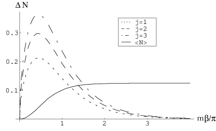
Figure 7: Plots of the fluctuation $\Delta N$, given in (39) and (40), for the special kink backgrounds in (34). The plots show the dependence of $\Delta N$ on the inverse temperature $\frac{m\beta}{\pi}$, for various values of the kink scale j, as indicated. This plot is for $\hat{\theta}=\pi/8$. The solid line shows the corresponding value of the fermion number $\langle N\rangle$, which is topological and therefore independent of the scale j. Notice that $\Delta N$ vanishes exponentially as the temperature approaches zero, while $\langle N\rangle$ saturates to its zero temperature value of $1/8$. These plots show the dependence of the fluctuation $\Delta N$ on the scale j, indicating that $\Delta N$ is nontopological.

Given this result (38) for the odd part of the resolvent, the contour integral expression (33) for the fluctuation yields a summation expression:

$$(\Delta N)_{\rm T}^{2} = \frac{2m\beta|\sin\hat{\theta}|}{\pi^{3}}\,\sum_{n=0}^{\infty}\left\{{2(2n+1)^{4}\cos^{2}\hat{\theta}-(\frac{m\beta}{\pi})^{2}\left[(\frac{m\beta}{\pi})^{2}-(2n+1)^{2}\right]\over\left[(\frac{m\beta}{\pi})^{2}+(2n+1)^{2}\right]^{2}\left[(\frac{m\beta}{\pi})^{2}+(2n+1)^{2}\cos^{2}\hat{\theta}\right]^{3/2}}\right.$$ (39)

$$\left.+2\sum_{l=1}^{j-1}\left(\frac{l}{j}\right)\,{2(2n+1)^{4}\cos^{2}\hat{\theta}-(\frac{m\beta}{\pi})^{2}\left[(\frac{m\beta}{\pi})^{2}-(2n+1)^{2}\right]-(\frac{m\beta}{\pi})^{4}(1-\frac{l^{2}}{j^{2}})\tan^{2}\hat{\theta}\over\left[(\frac{m\beta}{\pi})^{2}\left(1+(1-\frac{l^{2}}{j^{2}})\tan^{2}\hat{\theta}\right)+(2n+1)^{2}\right]^{2}\left[(\frac{m\beta}{\pi})^{2}+(2n+1)^{2}\cos^{2}\hat{\theta}\right]^{3/2}}\right\}$$

Alternatively, there is an equivalent integral representation expression:

$$(\Delta N)_{\rm T}^{2} = \frac{1}{4}\left\{{\rm sech}^{2}(\frac{m\beta}{2})-\frac{2|\sin\hat{\theta}|}{\pi}\int_{1}^{\infty}du\,{u\,{\rm sech}^{2}\left(\frac{m\beta}{2}{\rm sec}\hat{\theta}\,u\right)\over(u^{2}-\cos^{2}\hat{\theta})\sqrt{u^{2}-1}}\right.$$ (40)

$$\hskip-113.81102pt+2\sum_{l=1}^{j-1}\left.\left[{\rm sech}^{2}\left(\frac{m\beta}{2}\sqrt{1+(1-\frac{l^{2}}{j^{2}})\tan^{2}\hat{\theta}}\right)-\frac{2|\sin\hat{\theta}|}{\pi}\left(\frac{l}{j}\right)\,\int_{1}^{\infty}du\,{u\,{\rm sech}^{2}\left(\frac{m\beta}{2}{\rm sec}\hat{\theta}\,u\right)\over\left(u^{2}-(1-\frac{l^{2}}{j^{2}}\sin^{2}\hat{\theta})\right)\sqrt{u^{2}-1}}\right]\right\}$$

The fluctuations are plotted in Fig. 7 for $\hat{\theta}=\frac{\pi}{8}$, and various values of the scale parameter $j$. It is clear that the fluctuation vanishes exponentially at zero temperature ($m\beta\to\infty$). It is also clear that the fluctuation is nontopological, as it depends on the scale parameter $j$. At low temperature, the leading behavior is independent of the scale $j$

$$(\Delta N)_{\rm T}^{2}\sim e^{-m\beta}+\dots,$$ (41)

but the subleading exponential corrections are $j$ dependent, as can be seen from the integral expression (40) and from the plots in Fig. 7.

IV.2 Fluctuations in Sigma Model Case

In the sigma model case, there is no exact expression for either the odd or the even part of the Dirac resolvent. However, applying the derivative expansion as in ad , we find that in the low temperature ($T\ll m$) limit the dominant contribution comes from terms involving (even) powers of $\theta^{\prime}(x)$. These can be evaluated and resummed to all orders of the derivative expansion, to yield the leading low temperature result :

$$(\Delta N)_{\rm T}^{2}\,\sim\,2\sqrt{\frac{2mT}{\pi}}\,e^{-m/T}\,\int dx\,\sinh^{2}\left(\frac{\theta^{\prime}}{4T}\right)+\dots$$ (42)

This expression has a smooth low temperature limit in the derivative expansion regime where $\theta^{\prime}\ll m$. Indeed, the fluctuation (42) vanishes as $T\to 0$. Furthermore, at any finite temperature, the fluctuation (42) is clearly nontopological. In the next Section we will see that this expression for the fluctuation has a simple plasma interpretation, analogous to the linear response explanation (28) – (31) of the induced fermion number (25) in the sigma model case.

V Physical Interpretation

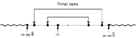
Figure 8: The general structure of the Dirac spectrum for a kink background. There is a single unpaired bound state at $E=-m$. (This assumes $\hat{\theta}>0$. If $\hat{\theta}<0$, then the unpaired bound state would be at $E=+m$.) There are continuum thresholds at $E=\pm m\,{\rm sec}\hat{\theta}=\pm\sqrt{m^{2}+\hat{\phi}_{2}^{2}}$. There may or may not be additional bound states with energies in the range $m<|E|<m\,{\rm sec}\hat{\theta}$, but if these states are present they are necessarily paired in $\pm E$ pairs.

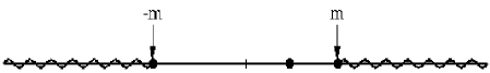
Figure 9: The structure of the Dirac spectrum for a sigma model background. The only general thing that can be said is that the continuum thresholds appear at $E=\pm m$. There is no particular symmetry to the spectrum, and there may or may not be one or more bound states in the gap. This depends sensitively on the detailed form of the angular field $\theta(x)$.

In this Section we give a simple physical interpretation of the results of the previous Sections for the induced fermion number and its fluctuations, in terms of the spectrum of the fermions in the background field. Let us first summarize the results. At zero temperature, the induced fermion number $\langle N\rangle_{0}$ is always topological, and has vanishing fluctuation: $(\Delta N)_{0}=0$. At finite temperature, $\langle N\rangle_{\rm T}$ is topological for a kink background, but nontopological for a sigma model background. For both the kink and sigma model cases, the fluctuation is non-vanishing, $(\Delta N)_{\rm T}\neq 0$, at nonzero temperature, and $(\Delta N)_{\rm T}$ is nontopological. The vanishing of the fluctuations at zero temperature is in agreement with previous arguments that the zero temperature induced fermion number is a sharp observable kivelson ; bell ; jackiw ; frishman ; charge . At finite temperature, the nonvanishing fluctuation indicates that the induced fermion number is no longer a sharp observable. Rather, it is a thermal expectation value that mixes contributions from different states in the fermion Hilbert space. This is somewhat analogous to the recent observation of Jackiw et al helium that fractional electron number in liquid helium bubbles is not sharp, due to state mixing.

In the sigma model case, the resummed derivative expansion result (25) for $\langle N\rangle_{\rm T}$ suggested a natural separation of the finite temperature induced fermion number $\langle N\rangle_{\rm T}$ into a zero temperature topological piece $\langle N\rangle_{0}$ and a nontopological piece that represents the plasma response to the background field (in this case, an inhomogeneous electric field). This separation is, in fact, a general feature of the induced fermion number: $\langle N\rangle_{\rm T}$ splits into a topological piece $\langle N\rangle_{0}$ that arises due to vacuum polarization effects (and only involves the ground state of the second quantized Hilbert space), and a nontopological piece that can be interpreted in terms of the thermal occupation numbers of nonvacuum states. The topological piece is temperature independent, while the nontopological piece is temperature dependent. To see how this separation arises, note the simple identity

$$\tanh\left(\frac{\beta E}{2}\right)=1-2n(E)$$ (43)

where the Fermi occupation number distribution is

$$n(E)=\frac{1}{e^{\beta E}+1}$$ (44)

Then the finite temperature induced fermion number (10) separates as

$$\langle N\rangle_{\rm T} = -\frac{1}{2}\int_{-\infty}^{\infty}dE\,\sigma(E)\,{\rm sign}(E)+\int_{-\infty}^{\infty}dE\,\sigma(E)\,{\rm sign}(E)\,n(|E|)$$ (45)

The first term in (45) is just the zero temperature fermion number (8), and is topological. However, the fact that the spectral asymmetry integral in (8) is always topological does not necessarily mean that $\sigma_{\rm odd}(E)$ is itself topological. The second term in (45) is generically nontopological due to the weighting of the integral with the Fermi distribution factor. However, in the special case of a kink background, $\sigma_{\rm odd}(E)$ is itself topological [see the Callias index theorem result (14)]. Thus the temperature-dependent second term in (45) is also topological in the kink case, even though the integral involves the Fermi factor.

This separation can be understood in terms of the Dirac spectrum of the fermions in the given background. For example, in the kink case, the Sommerfeld-Watson integral representation (18) for the induced fermion number can be re-expressed using (19), (43) and (45) as:

$$\langle N\rangle_{\rm T}=\langle N\rangle_{0}-{\rm sign}(\hat{\theta})\,n(m)+\frac{2m^{2}\tan\hat{\theta}}{\pi}\int_{m{\rm sec}\hat{\theta}}^{\infty}dE\,\frac{n(E)}{(E^{2}-m^{2})\sqrt{E^{2}-m^{2}{\rm sec}^{2}\hat{\theta}}}$$ (46)

For any kink background (with $\hat{\theta}$ positive), the spectrum of the Dirac Hamiltonian (6) always has the form shown in Fig. 8. There are continuum states for $|E|>\sqrt{m^{2}+\hat{\phi}_{2}^{2}}=m\,{\rm sec}\,\hat{\theta}$, where we recall that $\hat{\theta}\equiv{\rm arctan}(\hat{\phi_{2}}/m)$, and $\hat{\phi_{2}}$ is the asymptotic value of the kink field at $x=+\infty$. In addition, there is always a bound state at $E=-{\rm sign}(\hat{\theta})\,m$:

$$\psi_{b} = \left(\matrix{0\cr\exp[-\int^{x}\phi_{2}]}\right)\quad{\rm with\,\,energy}\,\,E=-m,\,\,{\rm if}\,\,\hat{\theta}>0$$

$$\psi_{b} = \left(\matrix{\exp[\int^{x}\phi_{2}]\cr 0}\right)\quad{\rm with\,\,energy}\,\,E=+m,\,\,{\rm if}\,\,\hat{\theta}<0$$ (47)

There may or may not be additional bound states with $m<|E|<m\,{\rm sec}\,\hat{\theta}$. If these additional bound states are present they necessarily occur in $\pm E$ pairs, because of the quantum mechanical SUSY of the Dirac Hamiltonian (6) in the kink case. Thus, the contributions of these paired bound states to the second integral in (45) cancel in pairs, while the unpaired bound state at $E=-{\rm sign}(\hat{\theta})\,m$ leads to the $-{\rm sign}(\hat{\theta})\,n(m)$ term in (46). The remaining integral over the continuum states leads to the integral term in (46), as an integral of the Fermi factor $n(|E|)$ over the continuum beginning at the threshold energy $m{\rm sec}\hat{\theta}$, with the integrand involving the odd part of the spectral function derived from the Callias index theorem result (14).

In the sigma model case, the Dirac spectrum is very different. As discussed in Section III.B, the chiral field $\theta(x)$ is equivalent to a spatially inhomogeneous electric field $E(x)=-\frac{1}{2}\theta^{\prime\prime}(x)$ for fermions of mass $m$. For a slowly varying background, with $\theta^{\prime}\ll m$, the leading order effect on the spectrum is that of a local chemical potential $\mu(x)=-\frac{1}{2}\theta^{\prime}(x)$. Thus, we can approximate (45) as

$$\langle N\rangle_{\rm T} \approx \langle N\rangle_{0}+\int_{-\infty}^{\infty}dx\int_{-\infty}^{\infty}\frac{dk}{2\pi}\,\left(\frac{1}{e^{\beta(\sqrt{k^{2}+m^{2}}+\theta^{\prime}/2)}+1}-\frac{1}{e^{\beta(\sqrt{k^{2}+m^{2}}-\theta^{\prime}/2)}+1}\right)$$ (48)

$$\sim \langle N\rangle_{0}-\sqrt{\frac{2mT}{\pi}}\,e^{-m/T}\,\int_{-\infty}^{\infty}dx\,\sinh\left(\frac{\theta^{\prime}}{2T}\right)\quad,\quad{\rm as}\quad T\to 0$$

which agrees precisely with the low temperature resummed derivative expansion result (25), and which agrees with the plasma linear response result as explained in Section III.B.

From numerical analysis of the Dirac equation for a sigma model background, the Dirac spectrum has the form shown in Fig. 9. Note that, unlike the kink case spectrum depicted in Fig. 8, there is no particular symmetry of the spectrum. The only general thing we can say is that the continuum thresholds are at $E=\pm m$. There may or may not be one or more bound states for $|E|<m$. The existence of (and the precise location of) bound states is highly sensitive to the actual shape of the $\theta(x)$. As there is no special symmetry in the spectrum, there is nothing general that can be said about the odd part of the spectral function. Nevertheless, the first term in (45), which is $\langle N\rangle_{0}$, yields a topological result since the integral can be written, using Levinson’s theorem, in terms of the phase shift at infinity, which is topological yamagishi ; boy ; mike ; jaffe2 . This application of Levinson’s theorem doesn’t work for the second term in (45) because of the Fermi factor. This is another way to understand why the finite temperature induced fermion number is generically nontopological. At low temperature, we see from (45) that the dominant correction to the zero temperature fermion number is determined by the bound state energy with the lowest magnitude:

$$\langle N\rangle_{\rm T}\sim\langle N\rangle_{0}+{\rm sign}(E_{\rm min})\,e^{-\beta\,|E_{\rm min}|}+\dots\quad,\quad{\rm as}\quad T\to 0$$ (49)

Since the location of $E_{\rm min}$ is sensitive to the detailed shape of $\theta(x)$, this shows that $\langle N\rangle_{\rm T}$ is generically nontopological. If there is no bound state, then the leading correction comes from the threshold and is $\sim e^{-m\beta}$, with nontopolgical subleading corrections.

The fluctuation (33) can also be expressed in terms of the Fermi distribution functions $n(E)$ in (44). Noting the simple identity

$$\frac{1}{4}\,{\rm sech}^{2}\left(\frac{\beta E}{2}\right)=n(E)\left(1-n(E)\right)$$ (50)

we see that (33) can be written as

$$(\Delta N)^{2}_{\rm T}=\int_{-\infty}^{\infty}dE\,\sigma(E)\,n(E)\,\left(1-n(E)\right)$$ (51)

This formula is natural, since it is well known pathria that for noninteracting fermions, the fluctuation in the occupation number of the state with energy $E$ is $\langle n^{2}_{E}\rangle-\langle n_{E}\rangle^{2}=\langle n_{E}\rangle\left(1-\langle n_{E}\rangle\right)$. In this paper we are considering the fermions to be in a fixed static background, so we are simply populating the single-particle energy levels of the corresponding Dirac Hamiltonian with noninteracting fermions, according to Fermi-Dirac statistics. This explains why the fluctuation vanishes at zero temperature, as the $n(1-n)$ factors vanish exponentially fast. It also explains why the fluctuation is nontopological, since the integral in (51) requires detailed knowledge of the spectrum.

For the family of special kink backgrounds in (34), the integral representation result (40) for the fluctuation can be re-expressed in terms of the Fermi occupation numbers of the states in the spectrum:

$$(\Delta N)^{2}_{\rm T} = n(m)\left(1-n(m)\right)+2\sum_{l=1}^{j-1}n(E_{l})\left(1-n(E_{l})\right)-\frac{2m|\tan\hat{\theta}|}{\pi}\int_{m{\rm sec}\hat{\theta}}^{\infty}dE\,\frac{E\,n(E)\left(1-n(E)\right)}{(E^{2}-m^{2})\sqrt{E^{2}-m^{2}{\rm sec}^{2}\hat{\theta}}}$$ (52)

$$-\frac{4m|\tan\hat{\theta}|}{\pi}\sum_{l=1}^{j-1}\,\left(\frac{l}{j}\right)\int_{m{\rm sec}\hat{\theta}}^{\infty}dE\,\frac{E\,n(E)\left(1-n(E)\right)}{(E^{2}-E_{l}^{2})\sqrt{E^{2}-m^{2}{\rm sec}^{2}\hat{\theta}}}$$

where the paired bound state energies $\pm E_{l}$ for the special kink backgrounds (34) are at

$$E_{l}=m\sqrt{1+(1-\frac{l^{2}}{j^{2}})\tan^{2}\hat{\theta}}\qquad,\qquad l=1,2,\dots,(j-1)$$ (53)

This expression (52) can be interpreted directly in terms of the general expression (51) : we can easily identify the separate contributions from the unpaired bound state at $E=-m$, from the paired bound states at $E=\pm E_{l}$, and the contributions from the continuum cuts. Since the integral in (51) involves the even part of the spectral function, the symmetry of the spectrum indicated in Fig. 8 does not lead to any particular simplification for the fluctuation, as there are no cancellations. Hence, $(\Delta N)_{\rm T}^{2}$ is nontopological, as it is manifestly dependent on the scale parameter $j$.

In the sigma model case, we can interpret the equation (51) as follows. As discussed previously, in the derivative expansion, $\theta^{\prime}\ll m$, limit, the leading effect of the background is that of a local chemical potential $\mu(x)=-\frac{1}{2}\theta^{\prime}(x)$, in which case the local Fermi distribution factors are given by (29). Thus, the fluctuation can be computed from (51) as

$$(\Delta N)^{2}_{\rm T} \approx \int dx\int_{-\infty}^{\infty}\frac{dk}{2\pi}\left[f_{+}(1-f_{+})+f_{-}(1-f_{-})-2f_{0}(1-f_{0})\right]$$ (54)

$$= \int dx\int_{-\infty}^{\infty}\frac{dk}{2\pi}\left[n(\sqrt{k^{2}+m^{2}}-\mu(x))\left(1-n(\sqrt{k^{2}+m^{2}}-\mu(x))\right)\right.$$

$$\left.+n(\sqrt{k^{2}+m^{2}}+\mu(x))\left(1-n(\sqrt{k^{2}+m^{2}}+\mu(x))\right)-2n(\sqrt{k^{2}+m^{2}})\left(1-n(\sqrt{k^{2}+m^{2}})\right)\right]$$

where the last term is the subtraction of the free case with $f_{0}=n(\sqrt{k^{2}+m^{2}})$. At low temperature, (54) gives the leading contribution

$$(\Delta N)^{2}_{\rm T} \approx \int dx\int_{-\infty}^{\infty}\frac{dk}{2\pi}\,e^{-\beta\sqrt{k^{2}+m^{2}}}\,\left[e^{-\beta\theta^{\prime}/2}+e^{\beta\theta^{\prime}/2}-2\right]$$ (55)

$$\sim 4\sqrt{\frac{mT}{2\pi}}\,e^{-m\beta}\,\int dx\,\sinh^{2}\left(\frac{\theta^{\prime}}{4T}\right)$$

where we have used the low temperature behavior of the $k$ integral in (31). This expression (55) agrees precisely with the resummed derivative expansion result (42) for the fluctuation.

VI Conclusions

To conclude, we reiterate that the finite temperature induced fermion number $\langle N\rangle_{\rm T}$ is generically nontopological, and is not a sharp observable. The induced fermion number naturally splits into a topological temperature-independent piece that represents the effect of vacuum polarization on the Dirac sea, and a nontopological temperature-dependent piece that represents the thermal population of the available states in the fermion spectrum, weighted with the appropriate Fermi-Dirac factors. As the temperature approaches zero, the nontopological terms vanish exponentially fast, and we regain smoothly the familiar topological results at zero temperature. But at nonzero temperature, the nontopological contribution is more sensitive to the details of the spectrum, and so is generically nontopological. This is illustrated explicitly by a derivative expansion calculation, which is resummed to all orders at low temperature, for the case of a sigma model background. The induced fermion number $\langle N\rangle_{\rm T}$ only depends on the odd part of the spectral function. This means the case of a kink background is special because the Dirac spectrum for a kink background is remarkably symmetric, and the odd part of the spectral function is itself a topological quantity, in the sense that it only depends on the asymptotic value of the kink field, rather than on the full details of the shape of the kink field. Thus, the kink case is non-generic, and the finite temperature induced fermion number is actually topological, albeit a complicated function of the temperature and the asymptotic value of the kink field. On the other hand, the fluctuation, $(\Delta N)_{\rm T}$, is determined by the even part of the spectral function, for which no general topological information is known. Thus, the fluctuations are always nontopological at finite temperature. We illustrated this explicitly with an exact solution for a special class of kink backgrounds, and with a derivative expansion calculation for the sigma model case. The fluctuation vanishes at zero temperature, which shows that the induced fermion number is a sharp eigenvalue at zero temperature, in agreement with the arguments of kivelson ; bell ; jackiw ; frishman ; charge . But at finite temperature, the nonvanishing of the fluctuations indicates that the induced fermion number is not a sharp eigenvalue at nonzero temperature. The source of the fluctuation is clearly the dispersion introduced by mixing states in the thermal average. An analogous example of an induced fermion number expectation value that is not sharp has been discussed recently in helium .

Some of these results generalize immediately to higher dimensional cases. For example, the dependence of $\langle N\rangle_{\rm T}$ on just the odd part of the spectrum means that if the background has the same SUSY isospectral features as the kink case, then the finite temperature induced fermion number will be topological. This was in fact found to be true in ad where the $3+1$ dimensional induced fermion number in the presence of a static $SU(2)$ ’t Hooft-Polyakov monopole was shown to have exactly the same form as in the $1+1$ dimensional kink case, with the identification of the asymptotic value of the kink with the asymptotic value of the magnitude of the monopole’s Higgs field. This gives an interesting finite temperature remnant of the quantum mechanical SUSY present in the Dirac spectrum. Conversely, without such a special symmetry of the Dirac spectrum, the finite temperature induced fermion number will be generically nontopological. So, for example, for a chiral $SU(2)$ sigma model with a Skyrme background in $3+1$ dimensions, it is well known from numerical work that the Dirac energy spectrum of the fermions is not symmetric, and the energy of a possible bound state (and indeed the number of bound states) is highly sensitive to the details of the shape of the radial hedgehog field ripka . Since the leading low temperature contribution to the finite temperature fermion number in (45) is determined by the lowest magnitude bound state energy [see (49)], this shows that in this case the finite temperature induced fermion number is nontopological. Likewise, the fact that the finite temperature fluctuation $(\Delta N)_{\rm T}$ depends on the even part of the spectral function indicates that this will be generally nontopological. Finally, the interpretation in terms of the fluctuations for individual energy levels in the spectrum shows that the fluctuation is nonzero at finite temperature, but vanishing at zero temperature. Thus, the induced fermion number is a sharp observable at zero temperature, but not at finite temperature. In particular, for a Skyrme background in $3+1$ dimensions, the finite temperature fermion number is not simply the (topological) winding number of the Skyrme field, but a much more complicated nontopological object.

- (1) R. Jackiw and C. Rebbi, “Solitons with Fermion Number 1/2”, Phys. Rev. D 13 (1976) 3398.
- (2) J. Goldstone and F. Wilczek, “Fractional Quantum Numbers on Solitons”, Phys. Rev. Lett. 47 (1981) 986.
- (3) R. Jackiw, “Fermion Fractionization in Physics”, in Quantum Structure of Space and Time, M. Duff and C.J. Isham (Eds.) (Cambridge Univ. Press, 1982); R. Jackiw, “Fractional Fermions”, Comments Nucl. Part. Phys. 13 (1984) 15.
- (4) A. Niemi and G. Semenoff, “Fermion Number Fractionization in Quantum Field Theory”, Phys. Rep. 135 (1986) 99.
- (5) A. J. Heeger, S. Kivelson, J. R. Schrieffer and W. P. Su, “Solitons in conducting polymers”, Rev. Mod. Phys. 60 (1988) 781.
- (6) R. Jackiw, “Effects of Dirac’s Negative Energy Sea on Quantum Numbers”, Dirac Prize Lecture, ICTP Trieste, March 1999, hep-th/9903255.
- (7) W. P. Su, J. R. Schrieffer, A. J. Heeger, “Solitons in Polyacetylene”, Phys. Rev. Lett. 42 (1979) 1698, “Soliton Excitations in Polyacetylene”, Phys. Rev. B 22 (1980) 2099.
- (8) M. Rice, “Charged II-Phase Kinks in Lightly Doped Polyacetylene”, Phys. Lett. A 71 (1979) 152.
- (9) R. Jackiw and J. R. Schrieffer, “Solitons with Fermion Number 1/2 in Condensed Matter and Relativistic Field Theories”, Nucl. Phys. B 190 FS3 (1981) 253.
- (10) J. Goldstone and R. L. Jaffe, “Baryon Number in Chiral Bag Models”, Phys. Rev. Lett. 51 (1983) 1518.
- (11) E. D’Hoker and E. Farhi, “Skyrmions and/in the weak interactions”, Nucl. Phys. B241 (1984) 109, “Decoupling a Fermion in the Standard Electro-Weak Theory”, Nucl. Phys. B 248 (1984) 77; E. D’Hoker and J. Goldstone, “The Derivative Expansion of the Fermion Number Current”, Phys. Lett. B 158 (1985) 429.
- (12) D. Diakonov, V. Petrov, P. Pobylitsa, “A Chiral Theory of Nucleons”, Nucl. Phys. B 306 (1988) 809; R. D. Ball, “Chiral Gauge Theory”, Phys. Rep. 182 (1989) 1.
- (13) R. MacKenzie and F. Wilczek, “Illustrations of Vacuum Polarization by Solitons”, Phys. Rev. D 30 (1984) 2194, “Examples of Vacuum Polarization by Solitons”, Phys. Rev. D 30 (1984) 2260.
- (14) F. Wilczek, “Adiabatic Methods in Field Theory”, in 1984 TASI Lectures in Elementary Particle Physics, Ann Arbor, D. Williams (Ed.).
- (15) H. Yamagishi, “Comment on ‘Fractional Quantum Numbers of Solitons”’, Phys. Rev. Lett. 50 (1983) 458.
- (16) R. Blankenbecler and D. Boyanovsky, “Fractional charge and spectral asymmetry in one dimension: a closer look”, Phys. Rev. D 31 (1985) 2089.
- (17) M. Stone, “An elementary derivation of one-dimensional fermion number fractionalization”, preprint ILL-TH-84-51, December 1984.
- (18) E. Farhi, N. Graham, R. L. Jaffe and H. Weigel, “Fractional and Integer Charges from Levinson’s Theorem”, Nucl. Phys. B595 (2001) 536.
- (19) M. Paranjape and G. Semenoff , “Spectral Asymmetry, Trace Identities and the Fractional Fermion Number of Magnetic Monopoles”, Phys. Lett. B132 (1983) 369.
- (20) A. Niemi and G. Semenoff, “Fractional Fermion Number at Finite Temperature”, Phys. Lett. B 135 (1984) 121.
- (21) V. Soni and G. Baskaran, “Depletion of Fractional Fermion Number of a Soliton at Finite Chemical Potential and Temperature”, Phys. Rev. Lett. 53 (1984) 523.
- (22) W. Keil, “Comment on Fractionally Charged Solitons at Finite Temperature and Chemical Potential”, Phys. Lett. A 106 (1984) 89.
- (23) C. Coriano and R. Parwani, “The Electric Charge of a Dirac Monopole at Nonzero Temperature”, Phys. Lett. B 363 (1995) 71.
- (24) G. Dunne and J. Feinberg, “Finite Temperature Effective Action in Monopole Background”, Phys. Lett. B 477 (2000) 474.
- (25) A. Goldhaber, R. Parwani and H. Singh, “On the Fractional Electric Charge of a Magnetic Monopole at Nonzero Temperature”, Phys. Lett. B 386 (1996) 207.
- (26) I. J. R. Aitchison and G. Dunne, “Nontopological Finite Temperature Induced Fermion Number”, Phys. Rev. Lett. 86 (2001) 1690.
- (27) S. Midorikawa, “Fractional Charge at Finite Temperature”, Prog. Theor. Phys. 69 (1983) 1831; “Fractional Fermion Number and its Thermal Effect”, Phys. Rev. D 31 (1985) 1499.
- (28) A. Niemi, “Topological Solitons in a Hot and Dense Fermi Gas”, Nucl. Phys. B 251 (1985) 155.
- (29) S. Kivelson and J. R. Schrieffer, “Fractional charge, a sharp quantum observable”, Phys. Rev. B 25 (1982) 6447.
- (30) R. Rajaraman and J. S. Bell, “On solitons with half integral charge”, Phys. Lett. 116 B (1982) 151, “On states, on a lattice, with half-integral charge”, Nucl. Phys. B220 [FS8] (1983) 1.
- (31) R. Jackiw, A. Kerman, I. Klebanov and G. Semenoff, “Fluctuations of Fractional Charge in Soliton Anti-Soliton Systems”, Nucl. Phys. B225 (1983) 233.
- (32) Y. Frishman and B. Horovitz, “Charge Fluctuations and Fractional Charge of Fermions in (1+1) Dimensions”, Phys. Rev. B27 (1983) 2565.
- (33) A. S. Goldhaber and S. Kivelson, “Local charge versus Aharonov-Bohm charge”, Phys. Lett. 255 B (1991) 445.
- (34) R. Jackiw, C. Rebbi and J. R. Schrieffer, “Fractional Electrons in Liquid Helium?”, cond-mat/0012370.
- (35) R. Pisarski, T.L. Trueman and M. Tytgat, “How changes with temperature”, Phys. Rev. D56 (1997) 7077, “Anomalous Amplitudes in a Thermal Bath”, Prog. Theor. Phys. Suppl. 131 (1998) 427.
- (36) F. Gelis and M. Tytgat, “Anomalous Processes at High Temperature and Density in a two-dimensional Linear Sigma Model”, Phys. Rev. D63 (2001) 016001.
- (37) G. Dunne, K. Lee and C. Lu, “The Finite Temperature Chern-Simons Coefficient”, Phys. Rev. Lett. 78 (1997) 3434.
- (38) S. Deser, L. Griguolo and D. Seminara, “Gauge Invariance, Finite Temperature and Parity Anomaly in D=3”, Phys. Rev. Lett. 79 (1997) 1976.
- (39) C. Fosco, G. Rossini and F. Schaposnik, “Induced Parity Breaking Term at Finite Temperature”, Phys. Rev. Lett. 79 (1997) 1980, Err. 79 (1997) 4296.
- (40) G. Dunne, “Aspects of Chern-Simons Theories”, in Les Houches 1998, Topological Aspects of Low Dimensional Systems, A. Comtet, F. David, Th. Jolicoeur and S. Ouvry (Eds), (Springer, 1999).
- (41) J. D. Bjorken and S. D. Drell, Relativistic Quantum Fields, (McGraw-Hill, New York, 1965).
- (42) C. Callias, “Index Theorems on Open Spaces”, Commun. Math. Phys. 62 (1978) 213.
- (43) I. J. R. Aitchison and C. Fraser, “Derivative Expansion of Fermion Determinants : Anomaly-induced Vertices, Goldstone-Wilczek Currents, and Skyrme Terms”, Phys. Rev. D 31 (1985) 2605.
- (44) M. Le Bellac, Thermal Field Theory (Cambridge, 1996), Section 6.4.
- (45) R. Pathria, Statistical Mechanics, (Pergamon Press, Oxford, 1972).
- (46) L. D. Landau and E. M. Lifshitz, Quantum Mechanics (Nonrelativistic Theory), (Pergamon Press, Oxford, 1977).
- (47) P. Morse and H. Feshbach, Methods of Theoretical Physics, Vol. II, (McGraw-Hill, New York, 1953).
- (48) N. Graham and R. L. Jaffe, “Energy, Central Charge, and the BPS Bound for 1+1 Dimensional Supersymmetric Solitons”, Nucl. Phys. B544 (1999) 432.
- (49) S. Kahana and G. Ripka, “Baryon density of quarks coupled to a chiral field”, Nucl. Phys. A429 (1984) 462; G. Ripka, Quarks bound by chiral fields: the quark structure of the vacuum and of light mesons and baryons, (Clarendon Press, Oxford, 1997).