Twistfield Perturbations of Vertex Operators in the $\mathbb{Z}_{2}$-Orbifold Model

Abstract:

We apply Kadanoff’s theory of marginal deformations of conformal field theories to twistfield deformations of $\mathbb{Z}_{2}$ orbifold models in K3 moduli space. These deformations lead away from the $\mathbb{Z}_{2}$ orbifold sub-moduli-space and hence help to explore conformal field theories which have not yet been understood. In particular, we calculate the deformation of the conformal dimensions of vertex operators for $h,\tilde{h}<1/2$ in second order perturbation theory.

1 Introduction

Orbifolds of torus models are a very promising starting point for the study of more complicated conformal field theories. The reason for that is that their structure is still very close to the one of their “mother theory”, the torus model, which is known very well. The whole untwisted sector of the theory is inherited from the torus model, only the behaviour of the twistfields provides quite some difficulties to understand. However, especially in the case of the abelian $\mathbb{Z}_{N}$ orbifolds, a lot of progress has already been made in understanding the conformal properties of and with twistfields, e.g. in [1], [2], [3], [4], [5], [6], [7], [8], [9], [10].

Now, our immediate interest lies in the K3 part of the moduli space of N=(4,4) superconformal theories with central charge c=(6,6), although the following considerations and calculations might as well be generalised to other moduli spaces with N=(2,2) supersymmetry. This part of the moduli space contains quite a few Gepner models and submoduli spaces corresponding to cyclic orbifolds of the N=(4,4) supertoroidal theories with central charge c=(6,6), but neither does it contain toroidal theories themselves nor is there anything known about the theories in the vast empty spaces between these known subvarieties (see e.g. [11], [12]).

The idea is to use the theory of deformations of conformal field theories developed by Kadanoff already in 1978 ([13], [14]) in order to gain information about theories lying close to known subvarieties in moduli space. Kadanoff’s theory gives a prescription how to calculate a correlator in a theory which is deformed away from a known theory by an exactly marginal operator in terms of integrals over correlation functions in the known theory. As a conformal field theory in this moduli space is completely determined by the conformal weights and the three point correlation functions of its fields, it is sufficient to study their behaviour under deformations.

The aim of this article is to study the deformation of the conformal weights of vertex operators with small conformal weights $h,\tilde{h}<1/2$ in directions corresponding to marginal twistfields in second order perturbation theory. We will carry out this calculation starting off from any point of the 16-dimensional $\mathbb{Z}_{2}$ orbifold hyperplane in the above mentioned K3 part of moduli space.

The outline of the article is as follows. First we derive the four point correlator, which we need for our calculation. This part contains quite a long and tedious calculation the result of which is given in $(\ref{eigentlich2})$. It follows a discussion of the singularities of this correlator and the necessary renormalisation procedure. Then, we present the numerical results of the integration, analyse these and show the implications for the moduli space of K3.

2 The correlator

In the following, we want to investigate certain deformations of $\mathbb{Z}_{2}$ orbifold theories at central charge $c=6$. These are unitary, superconformal orbifolds of toroidal theories with orbifold group $\mathbb{Z}_{2}$. The following correlators are all calculated in a certain $\mathbb{Z}_{2}$ orbifold model, if not denoted otherwise. According to Kadanoff [13], a deformation of such a theory is given by the addition of exactly marginal operators $O_{j}(w,\bar{w})$ to the action of the original theory. A general deformation of the action is given by $\int d^{2}w\;\sum_{j\in I}g_{j}O_{j}(w,\bar{w})$, where $I$ is the index set of all exact marginal operators and $g_{j}\in\mathbb{R}$ are some (suitably small) coupling coefficients.

Now, the two point function of two conformal fields is completely determined by the conformal weights of these fields (up to normalisation). Hence, the deformation of conformal weights is given by the deformation of the two point function of a field with itself. This leads Kadanoff to the first order calculation [13]

$$\!\!\!\!\!\!\!\!\!\frac{\partial}{\partial g_{i}}\;\langle\,\Phi_{\alpha}(x,\bar{x})\;\Phi_{\alpha}(0,0)\,\rangle_{\bf g}\;\Big{|}_{{\bf g}=0}$$ (1)

$$=\left(-2\frac{\partial h(g_{i})}{\partial g_{i}}\log(x)-2\frac{\partial\tilde{h}(g_{i})}{\partial g_{i}}\log(\bar{x})\right)\;\langle\,\Phi_{\alpha}(x,\bar{x})\;\Phi_{\alpha}(0,0)\,\rangle_{0}\;$$

$$=\int\mbox{d}^{2}w\;\langle\,O_{i}(w,\bar{w})\Phi_{\alpha}(x,\bar{x})\;\Phi_{\alpha}(0,0)\,\rangle_{0}\;,$$

where the $O_{i}(w,\bar{w})$ denote the exactly marginal operators (as above), $\langle\,.\,\rangle_{\bf g}$ the correlator in the deformed theory (deformed by $\sum_{j\in I}g_{j}O_{j}(w,\bar{w})$, ${\bf g}$ denotes the vector of the $g_{j}$) and $h,\tilde{h}$ the conformal weights of $\Phi_{\alpha}$ w.r.t. the left resp. right Virasoro field. But, taking $O_{i}(w,\bar{w})$ to be an exactly marginal twistfield and $\Phi_{\alpha}(x,\bar{x})$ to be a bosonic vertex operator, this order of perturbation theory naturally vanishes due to the point group selection rule. The point group selection rule requires that all twists of the correlator sum up to an integer number. In the case of the orbifold group $\mathbb{Z}_{2}$ that means that we always need an even number of twistfields in a correlator. (See e.g. [5] for an introduction to conformal field theory on cyclic orbifolds.) However, as long as all orders in perturbation theory have vanished up to the $n^{\mbox{\tiny th}}$ order, the result in $(\ref{direkt})$ can easily be generalised to the $(n\!+\!1)^{\,\mbox{\tiny st}}$ order

$$\!\!\!\!\!\!\!\!\!\frac{\partial^{n+1}}{\partial g_{i}^{n+1}}\;\langle\,\Phi_{\alpha}(x,\bar{x})\;\Phi_{\alpha}(0,0)\,\rangle_{\bf g}\;\Big{|}_{{\bf g}=0}=$$ (2)

$$= \left(-2\frac{\partial^{n+1}h}{\partial g_{i}^{n+1}}\log(x)-2\frac{\partial^{n+1}\tilde{h}}{\partial g_{i}^{n+1}}\log(\bar{x})\right)\;\langle\,\Phi_{\alpha}(x,\bar{x})\;\Phi_{\alpha}(0,0)\,\rangle_{0}$$

$$= \int\mbox{d}^{2}w_{1}\ldots\int\mbox{d}^{2}w_{n+1}\;\langle\,\Phi_{\alpha}(x,\bar{x})\;\Phi_{\alpha}(0,0)O_{i}(w_{1})\ldots O_{i}(w_{n+1})\,\rangle_{0,c}\;\;,$$

where the last correlator only contains the connected part, i.e. all contributions to this correlator originating in a factorisation of the correlator into two or more correlators have to be subtracted, and where the integral has to be suitably regulated by a cut-off. Hence, we can proceed to calculate the second order perturbation of the conformal weights by calculating the corresponding four point correlation function first.

The four point correlation function of two vertex operators with two ground state twistfields in $\mathbb{Z}_{2}$ orbifolds of toroidal theories has been known for quite a while (see e.g. [3], [9], [10]; a short derivation can be found in the appendix). However, doing perturbation theory with twistfields, the proper marginal operators to perturb a correlation function are not the (anti-)chiral ground state twistfields in the NSNS sector with conformal dimension $h,\tilde{h}=1/2$ but their superpartners. Only these have the right conformal dimensions $h,\tilde{h}=1$ and are exactly marginal to all orders in perturbation theory [5].

We take the $\mathbb{Z}_{2}$ orbifold group to act on the holomorphic U(1) currents $j_{s}(z)=i\partial X_{s}$ of the underlying toroidal theory by multiplication with a minus sign, i.e. $j_{s}(z)\mapsto-j_{s}(z)$. Hence, the vector of U(1) charges $p$ of the torus vertex operators $V^{t}_{p}$ w.r.t. to these toroidal U(1) currents is also multiplied with a minus sign under this group action. The vertex operators are mapped $V^{t}_{p}\mapsto V^{t}_{-p}$. The superscript $t$ signifies a field of the original torus theory. Thus, the $\mathbb{Z}_{2}$ orbifold model only contains the symmetrical linear combinations of torus vertex operators

$$V_{p}=\frac{1}{\sqrt{2}}\left(V^{t}_{p}+V^{t}_{-p}\right)\;,$$

as these are invariant under the group action. As we always work in even real dimensions, we will often use the linear combinations $j^{(k)}_{\pm}=\frac{1}{\sqrt{2}}(j_{k}\pm ij_{k+d/2})$ for the bosonic currents of the torus theory, and for the charges $p\equiv(p^{(k)}_{+},p^{(k)}_{-})_{k=1\dots d/2}$ respectively. The upper index in brackets $k=1\dots d/2$ signifies the complex dimension, the lower index $s=1\dots d$ the real dimension. The normalisation of the $V_{p}^{t}$ is fixed in the appendix.

In order to build correct marginal operators for a unitary deformation of the toroidal theory, we first take the hermitian linear combinations of ground state twistfields $\frac{1}{\sqrt{2}}(T_{+1/2}^{f}+T_{-1/2}^{f})$ where $f$ signifies the fixed point at which the respective field is localised, where the $\pm$ sign indicates whether this field belongs to an (anti)twist and where $k/N=1/2$ gives the corresponding twist itself. (For an introduction to cyclic orbifolds and the fields in the twisted sectors we refer to e.g. [5].) We find the proper exactly marginal twistfields as their (left+right) superpartners with conformal dimensions $h,\tilde{h}=1$, represented by

$$S^{f}=\frac{1}{\sqrt{2}}(S_{+1/2}^{f}+S_{-1/2}^{f})\;.$$

For ease of notation, we will omit the superscript $f$ in the following; it is understood that all twistfields live at the same fixed point.

Now, we can start to calculate the correlator

$$Z \equiv \langle\,V_{p}(z,\bar{z})\;V_{-p}(w,\bar{w})\;S(x,\bar{x})\;S(y,\bar{y})\,\rangle$$ (3)

$$= \langle\,V_{p}(z,\bar{z})\;V_{-p}(w,\bar{w})\;S_{+1/2}(x,\bar{x})\;S_{-1/2}(y,\bar{y})\,\rangle$$

$$= \bigg{\langle}\,V_{p}(z,\bar{z})\;V_{-p}(w,\bar{w})\;\left(\oint_{x}\mbox{d}\xi\;G^{-}(\xi)\oint_{\bar{x}}\mbox{d}\bar{\xi}\;\tilde{G}^{-}(\bar{\xi})\;T_{+1/2}(x,\bar{x})\;\right)$$

$$\left(\oint_{y}\mbox{d}\eta\;G^{+}(\eta)\oint_{\bar{y}}\mbox{d}\bar{\eta}\;\tilde{G}^{+}(\bar{\eta})\;T_{-1/2}(y,\bar{y})\right)\,\bigg{\rangle}\;$$

as part of the desired correlator. The first equality follows because the correlator with $S_{+1/2}$ and $S_{-1/2}$ interchanged will turn out to give exactly the same result as the one in the second line above and because these are the only two non-vanishing terms by the point group selection rule. In the third line, we use the fact that the $S_{\pm 1/2}$ are the superpartners of the ground state twistfields $T_{\pm 1/2}$, and hence can be constructed by applying the suitable supercurrents $G^{\pm}(\eta)$, $\tilde{G}^{\pm}(\eta)$ of the N=(2,2) Super–Virasoro–Algebra to the ground state twistfields. Notice that $T_{+1/2}$ is a chiral/chiral primary, $T_{-1/2}$ an antichiral/antichiral primary field.

There are two important things to notice. First, as we are dealing with a correlator containing only two twistfields, there are no classical solutions to be taken into account. Hence, the holomorphic and the antiholomorphic part of the correlator factorise. We will therefore concentrate on the holomorphic part in the following. Second, performing the supersymmetry transformations on the ground state twistfields themselves we run into deep problems as excited twistfields turn up whose correlation functions are rather nasty to handle and which have not been studied much so far. Hence, the idea is to take the contours of the integrals in $(\ref{eigentlich})$ not around a single twistfield but around all other fields in the correlator instead. This ’turning around of the contour’ gives a negative sign. As the supercurrents $G^{\pm}$ drop off as $1/z^{3}$ at infinity, there is no contribution at infinity. Now, taking into account the negative sign when interchanging two fermionic fields and noticing that there are only finite contributions in the OPE of $G^{+}(\eta)$ and the chiral primary field $T_{+1/2}(x)$, we get for the holomorphic factor

$$\tilde{Z} \equiv \bigg{\langle}\,V_{p}(z)\;V_{-p}(w)\;\left(\oint_{x}\mbox{d}\xi\;G^{-}(\xi)\;T_{+1/2}(x)\right)\;\left(\oint_{y}\mbox{d}\eta\;G^{+}(\eta)\;T_{-1/2}(y)\right)\,\bigg{\rangle}$$ (4)

$$= \frac{1}{2}\bigg{[}\bigg{\langle}\,\left(\left(\oint_{z}\mbox{d}\xi\;G^{-}(\xi)\;\oint_{z}\mbox{d}\eta\;G^{+}(\eta)-\oint_{z}\mbox{d}\eta\;G^{+}(\eta)\;\oint_{z}\mbox{d}\xi\;G^{-}(\xi)\right)V_{p}(z)\right)\;$$

$$V_{-p}(w)\;T_{+1/2}(x)\;T_{-1/2}(y)\,\bigg{\rangle}$$

$$+\bigg{\langle}\,\left(V_{p}(z)\left(\oint_{w}\mbox{d}\xi\;G^{-}(\xi)\;\oint_{w}\mbox{d}\eta\;G^{+}(\eta)-\oint_{w}\mbox{d}\eta\;G^{+}(\eta)\;\oint_{w}\mbox{d}\xi\;G^{-}(\xi)\right)V_{-p}(w)\;\right)$$

$$\;T_{+1/2}(x)\;T_{-1/2}(y)\,\bigg{\rangle}$$

$$+\bigg{\langle}\,V_{p}(z)\;V_{-p}(w)\;\left(\oint_{x}\mbox{d}\eta\;G^{+}(\eta)\;\oint_{x}\mbox{d}\xi\;G^{-}(\xi)T_{+1/2}(x)\right)\;T_{-1/2}(y)\,\bigg{\rangle}$$

$$-\bigg{\langle}\,V_{p}(z)\;V_{-p}(w)\;T_{+1/2}(x)\left(\oint_{y}\mbox{d}\xi\;G^{-}(\xi)\;\oint_{y}\mbox{d}\eta\;G^{+}(\eta)\;T_{-1/2}(y)\right)\,\bigg{\rangle}$$

$$+2\;\bigg{\langle}\,\left(\oint_{z}\mbox{d}\xi\;G^{-}(\xi)V_{p}(z)\right)\left(\oint_{w}\mbox{d}\eta\;G^{+}(\eta)\;V_{-p}(w)\;\right)\;T_{+1/2}(x)\;T_{-1/2}(y)\,\bigg{\rangle}$$

$$-2\;\bigg{\langle}\,\left(\oint_{z}\mbox{d}\eta\;G^{+}(\eta)V_{p}(z)\right)\left(\oint_{w}\mbox{d}\xi\;G^{-}(\xi)\;V_{-p}(w)\;\right)\;T_{+1/2}(x)\;T_{-1/2}(y)\,\bigg{\rangle}\bigg{]}.$$

First, we look at the first two terms of $(\ref{lang})$. We define $\psi_{\pm}^{(i)}$ to be the fermionic superpartners of the bosonic currents $j_{\pm}^{(i)}$, introduced earlier, where $i=1\dots d/2$ with $d$ the real dimension, hence $d/2$ the complex dimension. The normalisation is given by the OPEs

$$\psi^{(i)}_{+}(z)\;\psi^{(j)}_{-}(w)\sim\frac{\delta^{ij}}{z-w}\quad,\quad\quad j^{(i)}_{+}(z)\;j^{(j)}_{-}(w)\sim\frac{\delta^{ij}}{(z-w)^{2}}\;.$$

Then, using the explicit expression for the supercurrents (see e.g. [15])

$$G^{\pm}(z) = \sqrt{2}\;\sum_{i=1}^{d/2}:\psi_{\pm}^{(i)}j_{\mp}^{(i)}:(z)\;,$$ (5)

we can calculate ($p^{2}=\sum_{k=1}^{d}p_{k}p_{k}=\sum_{i=1}^{d/2}(p_{+}^{(i)\;2}+p_{-}^{(i)\;2})$)

$$\bigg{\langle}\,\left(\oint_{z}\mbox{d}\xi\;G^{-}(\xi)\;\oint_{z}\mbox{d}\eta\;G^{+}(\eta)V_{p}(z)\right)\;V_{-p}(w)\;T_{+1/2}(x)\;T_{-1/2}(y)\,\bigg{\rangle}=$$ (6)

$$= \bigg{\langle}\,\left(\oint_{z}\mbox{d}\xi\;G^{-}(\xi)\;\sqrt{2}\sum_{i=1}^{2}\;p_{-}^{(i)}\;:\ \psi_{+}^{(i)}\frac{1}{\sqrt{2}}\left(V^{t}_{p}-V^{t}_{-p}\right):(z)\right)\;$$

$$V_{-p}(w)\;T_{+1/2}(x)\;T_{-1/2}(y)\,\bigg{\rangle}$$

$$= \bigg{\langle}\,\bigg{(}2\sum_{j=1}^{2}p_{-}^{(j)}\;\frac{1}{\sqrt{2}}:(j_{j}+ij_{j+d/2})\frac{1}{\sqrt{2}}\left(V^{t}_{p}-V^{t}_{-p}\right):(z)$$

$$+2\sum_{i,j=1}^{2}p_{+}^{(j)}p_{-}^{(i)}\;:\psi_{-}^{(j)}\psi_{+}^{(i)}V_{p}:(z)\bigg{)}\;V_{-p}(w)\;T_{+1/2}(x)\;T_{-1/2}(y)\,\bigg{\rangle}$$

$$= \bigg{\langle}\,\bigg{(}\partial_{z}V_{p}(z)+\sum_{k=1}^{2}\;:i\left(p_{k}\;j_{k+d/2}-p_{k+d/2}\;j_{k}\right)\frac{1}{\sqrt{2}}\left(V^{t}_{p}-V^{t}_{-p}\right):(z)$$

$$+p^{2}\left(-\frac{1}{2}\;\frac{1}{z-x}+\frac{1}{2}\;\frac{1}{z-y}\right)\;V_{p}(z)\bigg{)}\;V_{-p}(w)\;T_{+1/2}(x)\;T_{-1/2}(y)\,\bigg{\rangle}.$$

The derivative of the vertex operator cancels with the corresponding term in the expression with interchanged supercurrents in $(\ref{lang})$. The second term in $(\ref{eins})$ vanishes when applying the U(1) currents $j_{i}$ to the vertex operators, using the OPE

$$j_{i}(z)\;V^{t}_{\pm p}(w)\sim\pm\,p_{i}(z-w)^{-1}V^{t}_{\pm p}(w)$$

within the correlator. Only the third term in $(\ref{eins})$ does not cancel with corresponding expressions, but U(1) charge conservation ensures that only the terms with $i=j$ contribute. Let $s_{\pm 1/2}^{(i)}$ signify the fermionic part of the twistfields $T_{\pm 1/2}$ with conformal dimension $h,\tilde{h}=1/8$ in complex dimension $i$. Then the correlator leading to this third term in $(\ref{eins})$ is calculated in the relevant dimension according to

$$\langle\,:\psi_{-}^{(i)}(w)\;\psi_{+}^{(i)}(z):\;s_{+1/2}^{(i)}(x)\;s_{-1/2}^{(i)}(y)\,\rangle=$$

$$= \lim_{w\rightarrow z}\left[\langle\,:\psi_{-}^{(i)}(w)\;\psi_{+}^{(i)}(z):\;s_{+1/2}^{(i)}(x)\;s_{-1/2}^{(i)}(y)\,\rangle-\frac{\langle\,s_{+1/2}^{(i)}(x)\;s_{-1/2}^{(i)}(y)\,\rangle}{w-z}\right]$$

$$= \lim_{w\rightarrow z}\left[(w-z)^{-1}\frac{(w-y)^{1/2}(z-x)^{1/2}}{(w-x)^{1/2}(z-y)^{1/2}}(x-y)^{-1/4}-\frac{(x-y)^{-1/4}}{w-z}\right]$$

$$= \left(-\frac{1}{2}\;\frac{1}{z-x}+\frac{1}{2}\;\frac{1}{z-y}\right)\langle\,s_{+1/2}^{(i)}(x)\;s_{-1/2}^{(i)}(y)\,\rangle\;.$$

Analogous calculations lead to the total result for the first and the second term in $(\ref{lang})$

$$\!\!\!\!\!\!\!\!\!\!\!\!\!\!\!\!\!\!\!\!\!\!\!\!\!2\;\left(-\frac{p^{2}}{2}\;\frac{1}{z-x}+\frac{p^{2}}{2}\;\frac{1}{z-y}-\frac{p^{2}}{2}\;\frac{1}{w-x}+\frac{p^{2}}{2}\;\frac{1}{w-y}\right)$$ (7)

$$\quad\quad\quad\quad\quad\times\;\bigg{\langle}\,V_{p}(z)\;V_{-p}(w)\;T_{+1/2}(x)\;T_{-1/2}(y)\,\bigg{\rangle}\;.$$

Now, we turn to the third and fourth term in $(\ref{lang})$. We can use the (anti)chiral properties of $T_{\pm 1/2}$ (i.e. $\ G^{\pm}(\eta)\;T_{\pm 1/2}(z)\sim\;\mbox{finite}$) to add in terms with interchanged order of the contours, but equal sign. Then, the usual contour argument (see e.g. [16], [17]) together with the OPE of the two supercurrents (see e.g. [15]) gives e.g.

$$\!\!\!\!\!\!\!\!\!\!\!\!\!\!\!\!\!\!\!\!\!\!\!\bigg{\langle}\,V_{p}(z)\;V_{-p}(w)\;\bigg{(}\Big{(}\oint_{x}\mbox{d}\eta\;G^{+}(\eta)\;\oint_{x}\mbox{d}\xi\;G^{-}(\xi)$$ (8)

$$\!\!\!\!\!\!\!\!\!\!\!\!\!\!\!\!\!\!+\oint_{x}\mbox{d}\xi\;G^{-}(\xi)\;\oint_{x}\mbox{d}\eta\;G^{+}(\eta)\Big{)}\;T_{+1/2}(x)\bigg{)}\;T_{-1/2}(y)\,\bigg{\rangle}$$

$$= \bigg{\langle}\,V_{p}(z)\;V_{-p}(w)\;\left(\oint_{x}\mbox{d}\xi\;\oint_{\xi}\mbox{d}\eta\;G^{+}(\eta)G^{-}(\xi)T_{+1/2}(x)\right)\;T_{-1/2}(y)\,\bigg{\rangle}$$

$$= \bigg{\langle}\,V_{p}(z)\;V_{-p}(w)\;\left(\oint_{x}\mbox{d}\xi\;(2\;{\cal T}(\xi)+\partial_{\xi}J(\xi))T_{+1/2}(x)\right)\;T_{-1/2}(y)\,\bigg{\rangle}$$

$$= 2\;\partial_{x}\;\bigg{\langle}\,V_{p}(z)\;V_{-p}(w)\;T_{+1/2}(x)\;T_{-1/2}(y)\,\bigg{\rangle}\;,$$

where ${\cal T}(\xi)$ and $J(\xi)$ signify the Virasoro field and the U(1) current, respectively, of the N=2 superconformal algebra. The last step uses the conformal algebra of primary fields (e.g. [15]). Calculating the derivative of the correlator $(\ref{verkorr2})$ given in the appendix

$$\!\!\!\!\!\!\partial_{x}\bigg{\langle}\,V^{t}_{p}(z)\;V^{t}_{\mp p}(w)\;T_{+1/2}(x)\;T_{-1/2}(y)\,\bigg{\rangle}$$

$$= \partial_{x}\bigg{[}4^{-p^{2}}(x-y)^{-1+(p\mp p)^{2}/2}((z-x)(z-y)(w-x)(w-y))^{-p^{2}/2}$$

$$\times\quad\left(\frac{((z-x)^{1/2}(w-y)^{1/2}+(z-y)^{1/2}(w-x)^{1/2})^{2}}{(w-z)}\right)^{\pm p^{2}}\bigg{]}$$

$$= \bigg{(}\frac{\frac{(p\mp p)^{2}}{2}-1}{x-y}+\frac{p^{2}}{2}\;\frac{1}{z-x}+\frac{p^{2}}{2}\;\frac{1}{w-x}$$

$$\mp p^{2}\;\frac{(z-x)^{-1/2}(w-y)^{1/2}+(z-y)^{1/2}(w-x)^{-1/2}}{(z-x)^{1/2}(w-y)^{1/2}+(z-y)^{1/2}(w-x)^{1/2}}\bigg{)}$$

$$\times\bigg{\langle}\,V^{t}_{p}(z)\;V^{t}_{\mp p}(w)\;T_{+1/2}(x)\;T_{-1/2}(y)\,\bigg{\rangle}\;.$$

we get the total contribution of the third and fourth terms in $(\ref{lang})$

$$2\;(\partial_{x}-\partial_{y})\;\bigg{\langle}\,V_{p}(z)\;V_{-p}(w)\;T_{+1/2}(x)\;T_{-1/2}(y)\,\bigg{\rangle}=$$ (9)

$$= 2\;\bigg{(}2\;\frac{p^{2}-1}{x-y}+\frac{p^{2}}{2}\left(\frac{1}{z-x}+\frac{1}{w-x}-\frac{1}{z-y}-\frac{1}{w-y}\right)\bigg{)}$$

$$\times\bigg{\langle}\,V_{p}(z)\;V_{-p}(w)\;T_{+1/2}(x)\;T_{-1/2}(y)\,\bigg{\rangle}$$

$$+ 2\;\bigg{(}p^{2}(x-y)^{-1}(z-x)^{-1/2}(z-y)^{-1/2}(w-x)^{-1/2}(w-y)^{-1/2}\Big{(}(z-x)(w-y)$$

$$+(z-y)(w-x)\Big{)}+p^{2}(z-x)^{-1/2}(z-y)^{-1/2}(w-x)^{-1/2}(w-y)^{-1/2}(x-y)\bigg{)}$$

$$\times\bigg{\langle}\,\frac{1}{\sqrt{2}}\Big{(}V^{t}_{p}-V^{t}_{-p}\Big{)}(z)\;\frac{1}{\sqrt{2}}\Big{(}V^{t}_{p}-V^{t}_{-p}\Big{)}(w)\;T_{+1/2}(x)\;T_{-1/2}(y)\,\bigg{\rangle}\;.$$

Now, only the last two terms in $(\ref{lang})$ are still left. Again, using $(\ref{super})$ we get for the fifth term in $(\ref{lang})$

$$\bigg{\langle}\,\left(\oint_{z}\mbox{d}\xi\;G^{-}(\xi)V_{p}(z)\right)\left(\oint_{w}\mbox{d}\eta\;G^{+}(\eta)\;V_{-p}(w)\;\right)\;T_{+1/2}(x)\;T_{-1/2}(y)\,\bigg{\rangle}=$$

$$= \bigg{\langle}\,\bigg{(}\sum_{i=1}^{2}\sqrt{2}\left(\psi_{-}^{(i)}(z)p_{+}^{(i)}\right)\frac{1}{\sqrt{2}}\left(V_{p}^{t}-V_{-p}^{t}\right)(z)\bigg{)}$$

$$\bigg{(}\sum_{j=1}^{2}\sqrt{2}\left(\psi_{+}^{(j)}(w)p_{-}^{(j)}\right)\frac{1}{\sqrt{2}}\left(V_{p}^{t}-V_{-p}^{t}\right)(w)\bigg{)}\;T_{+1/2}(x)\;T_{-1/2}(y)\,\bigg{\rangle}$$

$$= 2\;\bigg{(}\sum_{i,j=1}^{2}p_{+}^{(i)}p_{-}^{(j)}\langle\,\psi_{-}^{(i)}(z)\psi_{+}^{(j)}(w)\prod_{b=1}^{2}s^{(b)}_{+1/2}(x)s^{(b)}_{-1/2}(y)\,\rangle\bigg{)}\bigg{(}\langle\,\prod_{b=1}^{2}s^{(b)}_{+1/2}(x)s^{(b)}_{-1/2}(y)\,\rangle\bigg{)}^{\!\!\!-1}\;$$

$$\times\bigg{\langle}\,\frac{1}{\sqrt{2}}\Big{(}V^{t}_{p}-V^{t}_{-p}\Big{)}(z)\;\frac{1}{\sqrt{2}}\Big{(}V^{t}_{p}-V^{t}_{-p}\Big{)}(w)\;T_{+1/2}(x)\;T_{-1/2}(y)\,\bigg{\rangle}$$

$$= p^{2}(z-w)^{-1}(z-x)^{-1/2}(z-y)^{1/2}(w-x)^{1/2}(w-y)^{-1/2}$$

$$\times\bigg{\langle}\,\frac{1}{\sqrt{2}}\Big{(}V^{t}_{p}-V^{t}_{-p}\Big{)}(z)\;\frac{1}{\sqrt{2}}\Big{(}V^{t}_{p}-V^{t}_{-p}\Big{)}(w)\;T_{+1/2}(x)\;T_{-1/2}(y)\,\bigg{\rangle}\;.$$

Adding in the similar contribution of the sixth term of $(\ref{lang})$, the last two terms together give

$$\!\!\!\!\!\!\bigg{\langle}\,\left(\oint_{z}\mbox{d}\xi\;G^{-}(\xi)V_{p}(z)\right)\left(\oint_{w}\mbox{d}\eta\;G^{+}(\eta)\;V_{-p}(w)\;\right)\;T_{+1/2}(x)\;T_{-1/2}(y)\,\bigg{\rangle}$$ (10)

$$-\;\bigg{\langle}\,\left(\oint_{z}\mbox{d}\eta\;G^{+}(\eta)V_{p}(z)\right)\left(\oint_{w}\mbox{d}\xi\;G^{-}(\xi)\;V_{-p}(w)\;\right)\;T_{+1/2}(x)\;T_{-1/2}(y)\,\bigg{\rangle}$$

$$= -2\;p^{2}(z-x)^{-1/2}(z-y)^{-1/2}(w-x)^{-1/2}(w-y)^{-1/2}(x-y)$$

$$\times\bigg{\langle}\,\frac{1}{\sqrt{2}}\Big{(}V^{t}_{p}-V^{t}_{-p}\Big{)}(z)\;\frac{1}{\sqrt{2}}\Big{(}V^{t}_{p}-V^{t}_{-p}\Big{)}(w)\;T_{+1/2}(x)\;T_{-1/2}(y)\,\bigg{\rangle}\;.$$

Adding the results of $(\ref{erster-zweiter})$, $(\ref{dritter-vierter})$ and $(\ref{fuenfter-sechster})$, the total result reads

$$\tilde{Z} = 2\;\frac{p^{2}-1}{x-y}\;\bigg{\langle}\,V_{p}(z)\;V_{-p}(w)\;T_{+1/2}(x)\;T_{-1/2}(y)\,\bigg{\rangle}$$ (11)

$$+ p^{2}(x-y)^{-1}(z-x)^{-1/2}(z-y)^{-1/2}(w-x)^{-1/2}(w-y)^{-1/2}$$

$$\times\Big{(}(z-x)(w-y)+(z-y)(w-x)\Big{)}$$

$$\times\bigg{\langle}\,\frac{1}{\sqrt{2}}\Big{(}V^{t}_{p}-V^{t}_{-p}\Big{)}(z)\;\frac{1}{\sqrt{2}}\Big{(}V^{t}_{p}-V^{t}_{-p}\Big{)}(w)\;T_{+1/2}(x)\;T_{-1/2}(y)\,\bigg{\rangle}\;.$$

As already remarked earlier, the calculation for the antiholomorphic part runs independently and in exactly the same fashion. Call $p_{l}$ the U(1) charge w.r.t. the left moving, i.e. holomorphic U(1) current, $p_{r}$ the U(1) charge for the right moving, i.e. antiholomorphic U(1) current. Hence, the total result for $(\ref{eigentlich})$ is given by

$$Z = \bigg{[}2\;\frac{p_{l}^{2}-1}{x-y}\;-p_{l}^{2}(x-y)^{-1}(z-x)^{-1/2}(z-y)^{-1/2}(w-x)^{-1/2}(w-y)^{-1/2}$$ (12)

$$\Big{(}(z-x)(w-y)+(z-y)(w-x)\Big{)}\bigg{]}$$

$$\times\bigg{[}2\;\frac{p_{r}^{2}-1}{\bar{x}-\bar{y}}\;-p_{r}^{2}(\bar{x}-\bar{y})^{-1}(\bar{z}-\bar{x})^{-1/2}(\bar{z}-\bar{y})^{-1/2}(\bar{w}-\bar{x})^{-1/2}(\bar{w}-\bar{y})^{-1/2}$$

$$\Big{(}(\bar{z}-\bar{x})(\bar{w}-\bar{y})+(\bar{z}-\bar{y})(\bar{w}-\bar{x})\Big{)}\bigg{]}$$

$$\times\bigg{\langle}\,V_{p}^{t}(z,\bar{z})\;V_{-p}^{t}(w,\bar{w})\;T_{+1/2}(x,\bar{x})\;T_{-1/2}(y,\bar{y})\,\bigg{\rangle}$$

$$+ \bigg{[}2\;\frac{p_{l}^{2}-1}{x-y}\;+p_{l}^{2}(x-y)^{-1}(z-x)^{-1/2}(z-y)^{-1/2}(w-x)^{-1/2}(w-y)^{-1/2}$$

$$\Big{(}(z-x)(w-y)+(z-y)(w-x)\Big{)}\bigg{]}$$

$$\times\bigg{[}2\;\frac{p_{r}^{2}-1}{\bar{x}-\bar{y}}\;+p_{r}^{2}(\bar{x}-\bar{y})^{-1}(\bar{z}-\bar{x})^{-1/2}(\bar{z}-\bar{y})^{-1/2}(\bar{w}-\bar{x})^{-1/2}(\bar{w}-\bar{y})^{-1/2}$$

$$\Big{(}(\bar{z}-\bar{x})(\bar{w}-\bar{y})+(\bar{z}-\bar{y})(\bar{w}-\bar{x})\Big{)}\bigg{]}$$

$$\times\bigg{\langle}\,V_{p}^{t}(z,\bar{z})\;V_{p}^{t}(w,\bar{w})\;T_{+1/2}(x,\bar{x})\;T_{-1/2}(y,\bar{y})\,\bigg{\rangle}\;.$$

For the calculation of the perturbation of the two-vertex-correlator, we now want to specialise to the case of small $p_{l}^{2},p_{r}^{2}<1$. The vector of the left moving and right moving U(1) charges can be shown to lie on an even integer charge lattice in the underlying toroidal theory, especially $p_{l}^{2}-p_{r}^{2}\in 2\,\mathbb{Z}$ (see e.g. [16]). As a direct consequence of the above assumption, we therefore deduce $p_{l}^{2}=p_{r}^{2}\equiv p^{2}$. The perturbation in second order, according to $(\ref{direkt2})$, $(\ref{eigentlich})$ and $(\ref{eigentlich2})$, simplifies to

$$\int\mbox{d}^{2}x\int\mbox{d}^{2}y\;Z=(z-w)^{-p_{l}^{2}}\;(\bar{z}-\bar{w})^{-p_{r}^{2}}\;\int\mbox{d}^{2}x\;\frac{\mid\!z-w\!\mid^{2}}{\mid\!x-z\!\mid^{2}\;\mid\!x-w\!\mid^{2}}\;(V_{1}+V_{2})\;,$$ (13)

where $V_{1}$ corresponds to the first term in the sum in $(\ref{eigentlich2})$, $V_{2}$ to the second, and where the integrals $V_{i}$ are given by

$$V_{1} \equiv 4^{-p_{l}^{2}-p_{r}^{2}}\;\int d^{2}\zeta\;\frac{1}{\mid\!1-\zeta\!\mid^{4}}\;\Big{(}2\;(p_{l}^{2}-1)-p_{l}^{2}\;\zeta^{-1/2}\;(1+\zeta)\Big{)}$$

$$\Big{(}2\;(p_{r}^{2}-1)-p_{r}^{2}\;\bar{\zeta}^{-1/2}\;(1+\bar{\zeta})\Big{)}\;\zeta^{-p_{l}^{2}/2}\;\bar{\zeta}^{-p_{r}^{2}/2}\;(1-\zeta)^{p_{l}^{2}}\;(1-\bar{\zeta})^{p_{r}^{2}}$$

$$\bigg{(}\frac{1+\zeta^{1/2}}{1-\zeta^{1/2}}\bigg{)}^{p_{l}^{2}}\;\bigg{(}\frac{1+\bar{\zeta}^{1/2}}{1-\bar{\zeta}^{1/2}}\bigg{)}^{p_{r}^{2}}$$

$$V_{2} \equiv 4^{-p_{l}^{2}-p_{r}^{2}}\;\int d^{2}\zeta\;\frac{1}{\mid\!1-\zeta\!\mid^{4}}\;\Big{(}2\;(p_{l}^{2}-1)+p_{l}^{2}\;\zeta^{-1/2}\;(1+\zeta)\Big{)}$$

$$\Big{(}2\;(p_{r}^{2}-1)+p_{r}^{2}\;\bar{\zeta}^{-1/2}\;(1+\bar{\zeta})\Big{)}\;\zeta^{-p_{l}^{2}/2}\;\bar{\zeta}^{-p_{r}^{2}/2}\;(1-\zeta)^{p_{l}^{2}}\;(1-\bar{\zeta})^{p_{r}^{2}}$$

$$\bigg{(}\frac{1-\zeta^{1/2}}{1+\zeta^{1/2}}\bigg{)}^{p_{l}^{2}}\;\bigg{(}\frac{1-\bar{\zeta}^{1/2}}{1+\bar{\zeta}^{1/2}}\bigg{)}^{p_{r}^{2}}\;;$$

the four point correlator calculated in the appendix has been plugged in explicitely. The simplification in $(\ref{int})$ uses the SL(2,$\mathbb{C}$) transformation

$$\zeta(\eta)=\frac{\eta-z}{\eta-w}\;\frac{x-w}{x-z}\;,$$

which maps $z\mapsto 0$, $w\mapsto w^{\prime}\rightarrow\infty$, $x\mapsto 1$ and $y\mapsto\zeta$.

Both integrals $V_{i}$ can be merged to a single integral over the two sheeted Riemann surface of $t\equiv\pm\sqrt{\zeta}$. However, this presentation would make the following discussion of singularities considerably harder.

3 Singularities

As explained below equation $(\ref{direkt2})$, we have to identify and subtract the disconnected part of the integrand of $(\ref{int})$ and suitably regulate the remaining integral. There are two sources of singularities in $(\ref{int})$ for the case of small $p^{2}\equiv p_{l}^{2}=p_{r}^{2}$. First, for $z\rightarrow w$ we have a mixing of the two vertex operators $V^{t}_{p}(z,\bar{z})$ and $V^{t}_{-p}(w,\bar{w})$ with the identity; furthermore, for $x\rightarrow y$ the two twistfields $S_{+1/2}(x,\bar{x})$ and $S_{-1/2}(y,\bar{y})$ also mix with the identity. This channel is responsible for the disconnected part of $(\ref{int})$ which produces the singularity $\mid\!1-\zeta\!\mid^{-4}$ in $V_{1}$. Second, for $z\rightarrow w$ the two vertex operators $V^{t}_{p}(z,\bar{z})$ and $V^{t}_{p}(w,\bar{w})$ mix with the vertex operator $V^{t}_{-2p}(z,\bar{z})$; the same mixing occurs for the two twistfields $S_{+1/2}(x,\bar{x})$ and $S_{-1/2}(y,\bar{y})$ for $x\rightarrow y$. This channel is responsible for the $\zeta\rightarrow 1$ singularity in $V_{2}$. To understand this seemingly unusual mixing of $S_{+1/2}(x,\bar{x})$ and $S_{-1/2}(y,\bar{y})$ with the vertex operator $V^{t}_{-2p}(z,\bar{z})$, we have a closer look at the orbifold construction itself. In the twisted sector, the momenta $p$ and $-p$ are identified by the action of the orbifold group and exactly this fact guarantees that the conservation of momentum is not violated in the above OPE.

These singularities call for a proper regularisation procedure. In position space, this regularisation is best achieved by introducing a cut-off $\epsilon\rightarrow 0$ around the singularities and by subtracting the singular parts in $\epsilon$. But this can be shown to be equivalent to the following much more practicable procedure. First, one subtracts the terms that cause these singularities from the integrand. Then, one can integrate this integrand over the whole complex plane and acquires the correct result. (By definition, a term which causes a singularity has to behave exactly as the original integrand close to the singularity, and the integration of this singular term over the whole plane, cut off with the same $\epsilon$ at the singularity, should only exhibit an $\epsilon$ dependence. This is hence the same $\epsilon$ dependence as the one of the integral of the original integrand cut off close to the same singularity.)

Now, we want to write down the precise form of these two singular terms which are to be subtracted. Using the correlator of two ground state twistfields

$$\langle\,T_{+1/2}(x,\bar{x})\;T_{-1/2}(y,\bar{y})\,\rangle=\mid\!x-y\!\mid^{-2}\;,$$

an analogous turning around of the contours as in the case of the full four point function $(\ref{vertex1})$ leads to the correlator of the superpartners

$$\langle\,S_{+1/2}(x,\bar{x})\;S_{-1/2}(y,\bar{y})\,\rangle=4\;\mid\!x-y\!\mid^{-4}\;.$$

Hence, the whole disconnected contribution to $V_{1}$ reads

$$\langle\,V_{p}^{t}(z,\bar{z})\;V_{-p}^{t}(w,\bar{w})\,\rangle\;\langle\,S_{+1/2}(x,\bar{x})\;S_{-1/2}(y,\bar{y})\,\rangle=4\;(z-w)^{-p_{l}^{2}}\;(\bar{z}-\bar{w})^{-p_{r}^{2}}\;\mid\!x-y\!\mid^{-4}\;.$$

Doing an SL(2,$\mathbb{C}$) transformation as above, we get our final result for this singular part of the integral

$$(z-w)^{-p_{l}^{2}}\;(\bar{z}-\bar{w})^{-p_{r}^{2}}\;\int\mbox{d}^{2}x\;\frac{\mid\!z-w\!\mid^{2}}{\mid\!x-z\!\mid^{2}\;\mid\!x-w\!\mid^{2}}\;V_{1}^{S}$$

with

$$V_{1}^{S}\equiv 4\;\int\mbox{d}^{2}\zeta\frac{1}{\mid\!1-\zeta\!\mid^{4}}\;.$$

$V_{1}^{S}$ is exactly the $\zeta\rightarrow 1$ singularity of $V_{1}$. But as we only want to integrate over the connected part of the total integrand in $(\ref{int})$, we have to replace $V_{1}$ by $V_{1}-V_{1}^{S}$; this does not contain any singularity any more.

The second singularity, the singular part of $V_{2}$, is given for $p^{2}\leq\frac{1}{2}$ by

$$V_{2}^{S}\equiv 16^{-p_{l}^{2}-p_{r}^{2}}\;4\;(2p_{l}^{2}-1)\;(2p_{r}^{2}-1)\;\int\mbox{d}^{2}\zeta\;(1-\zeta)^{2p_{l}^{2}-2}\;(1-\bar{\zeta})^{2p_{r}^{2}-2}\;.$$ (14)

For $\frac{1}{2}<p^{2}<1$, $V_{2}$ is even finite. We now want to show that this singularity really originates in the mixing with vertex operators of charge $\pm 2p$. First, we notice that the correlator of three vertex operators is given by conformal invariance

$$\langle\,V_{p}^{t}(z,\bar{z})\;V_{p}^{t}(w,\bar{w})\;V_{-2p}^{t}(\xi,\bar{\xi})\,\rangle=$$ (15)

$$= (z-w)^{p_{l}^{2}}\;(\bar{z}-\bar{w})^{p_{r}^{2}}\;(z-\xi)^{-2p_{l}^{2}}\;(\bar{z}-\bar{\xi})^{-2p_{r}^{2}}\;(w-\xi)^{-2p_{l}^{2}}\;(\bar{w}-\bar{\xi})^{-2p_{r}^{2}}\;.$$

Analogously, conformal invariance fixes the correlator of two groundstate twistfields with a vertex operator

$$\langle\,V_{2p}^{t}(\xi,\bar{\xi})\;T_{+1/2}(x,\bar{x})\;T_{-1/2}(y,\bar{y})\,\rangle=$$

$$= C\;(x-y)^{2\,p_{l}^{2}-1}\;(\bar{x}-\bar{y})^{2\,p_{r}^{2}-1}\;(x-\xi)^{-2\,p_{l}^{2}}\;(\bar{x}-\bar{\xi})^{-2\,p_{r}^{2}}\;(y-\xi)^{-2\,p_{l}^{2}}\;(\bar{y}-\bar{\xi})^{-2\,p_{r}^{2}}\;$$

and a similar calculation as for the full four point function leads to the corresponding result with supertwistfields

$$\langle\,V_{2p}^{t}(\xi)\;S_{+1/2}(x)\;S_{-1/2}(y)\,\rangle=$$ (16)

$$= 4\;C\;(2p_{l}^{2}-1)\;(2p_{r}^{2}-1)\;(x-y)^{2\,p_{l}^{2}-2}\;(\bar{x}-\bar{y})^{2\,p_{r}^{2}-2}\;(x-\xi)^{-2\,p_{l}^{2}}$$

$$\;(\bar{x}-\bar{\xi})^{-2\,p_{r}^{2}}\;(y-\xi)^{-2\,p_{l}^{2}}\;(\bar{y}-\bar{\xi})^{-2\,p_{r}^{2}}\;.$$

Even without doing the integration over $\xi$, one can identify the leading singularity in the product of $(\ref{teil1})$ and $(\ref{teil2})$ with the singular part of $V_{2}$ $(\ref{fuehr})$. This identification fixes the normalisation factor to $C=16^{-p_{l}^{2}-p_{r}^{2}}$. Further terms in this product of $(\ref{teil1})$ and $(\ref{teil2})$ give higher orders of $(x-y)$ for $x\rightarrow y$ and hence do not contribute to the singular part of the integral. The total regularisation for $V_{2}$ reads $V_{2}-V_{2}^{S}$ in the case $p^{2}\leq\frac{1}{2}$; for $\frac{1}{2}<p^{2}<1$ no regularisation is necessary.

As these two singularities are the only ones for small $p_{l}^{2}$, $p_{r}^{2}$, the total regularisation of $V_{1}+V_{2}$ in $(\ref{int})$ is given by

$$V \equiv (V_{1}-V_{1}^{S})+(V_{2}-V_{2}^{S})\quad\quad\quad\mbox{for}\;p^{2}\leq\frac{1}{2}$$

$$V \equiv (V_{1}-V_{1}^{S})+V_{2}\quad\quad\quad\quad\quad\mbox{for}\;\frac{1}{2}<p^{2}<1\;.$$ (17)

For larger $p_{l}^{2}\geq 1$ or $p_{r}^{2}\geq 1$, we encounter further singularities also for $\zeta\rightarrow 0$ and $\zeta\rightarrow\infty$. These are the result of a mixing of $V_{p}(w,\bar{w})$ and $S_{\pm}(x,\bar{x})$ with ground state twistfields (see e.g. [3] for a discussion of such processes on string theoretic grounds).

4 Results

We now want to calculate the perturbation $(\ref{int})$ subtracting the singularities as discussed in section 3. In order to perform the $x$-integral in $(\ref{int})$, we use the translational invariance of correlation functions to set $w=0$ and apply the SL(2,$\mathbb{C}$) transformation

$$\gamma:\quad\zeta^{\prime}(\zeta)=\frac{z\zeta}{z-\zeta}\quad\quad\quad\quad\gamma^{-1}:\quad\zeta(\zeta^{\prime})=\frac{z\zeta^{\prime}}{\zeta^{\prime}+z}$$

which maps $0$ to $0$ and $z$ to $z^{\prime}\mapsto\infty$. Introducing a proper cut-off $\epsilon$, the logarithmically divergent $x$-integral in $(\ref{int})$ can be calculated to

$$\int_{\mid\!x-z\!\mid>\epsilon\atop\mid\!x\!\mid>\epsilon}\mbox{d}^{2}x\;\frac{\mid\!z\!\mid^{2}}{\mid\!x-z\!\mid^{2}\;\mid\!x\!\mid^{2}}=2\pi\log\frac{\mid\!z\!\mid^{2}}{\epsilon^{2}}\;.$$

As shown in $(\ref{direkt2})$, these logarithmic divergencies correspond to the variation of the conformal dimension of the vertex operators $V_{p}(z,\bar{z})$.

$p^{2}$	V	$p^{2}$	V
0.00000	0.00000	0.26000	-0.71670
0.01000	-0.06111	0.272211	-0.71256
0.01562	-0.09401	0.277008	-0.71007
0.02250	-0.13281	0.280277	-0.70810
0.04000	-0.22487	0.284444	-0.70525
0.06250	-0.32982	0.294117	-0.69722
0.07840	-0.39543	0.302500	-0.68865
0.09000	-0.43903	0.30864	-0.68141
0.11111	-0.50954	0.36000	-0.58841
0.16000	-0.63164	0.40111	-0.47008
0.20250	-0.69395	0.44444	-0.29899
0.22145	-0.70917	0.49000	-0.06109
0.22438	-0.71084	0.50000	0.00000
0.22873	-0.71299	0.56250	0.46758
0.23529	-0.71548	0.64000	1.31499
0.24000	-0.71670	0.69444	2.17848
0.25000	-0.71775

Table 1: Numerical results

Hence, the whole information about the deformation is given in the integral $V$ as in $(\ref{num})$. We solved the integral numerically for various $p^{2}<1$ using the program Mathematica. However, although the integral converges there are still divergencies in the integrand which have to be taken care of. The regularised integral $V_{1}$ still contains divergencies of the form $(1-\zeta)^{-2}$ or $(1-\bar{\zeta})^{-2}$ which we handle by cutting out an $\epsilon$-ball around $\zeta=1$ of size $\epsilon=0.01$. Integration over the first terms of a Taylor expansion around $\zeta=1$ gives the approximation that the contribution of this ball to the total integral amounts to about $10^{-6}$. In order to handle the $\mid\!1-\zeta\!\mid^{-r}$, $r<2$, singularities in the regularised $V_{2}$, we subtract the expression

$$\tilde{V}^{S}_{2} \equiv 16^{-2p_{l}^{2}}\;4\;(2p^{2}-1)^{2}$$

$$\qquad\int\mbox{d}^{2}\zeta\;\mid\!1-\zeta\!\mid^{4p_{l}^{2}-4}\;\mid\!\zeta\!\mid^{-2p^{2}}$$

instead of $V_{2}^{S}$. $V_{2}-\tilde{V}^{S}_{2}$ behaves much better numerically and the difference $\tilde{V}^{S}_{2}-V_{2}^{S}$ is known as Virasoro Shapiro amplitude in the literature (see e.g. [16])

$$\tilde{V}^{S}_{2}-V_{2}^{S} = 16^{-2p^{2}}\;4\;(2p^{2}-1)^{2}\;\int\mbox{d}^{2}\zeta\;\mid\!1-\zeta\!\mid^{4p^{2}-4}\left(\mid\!\zeta\!\mid^{-2p^{2}}-1\right)$$ (18)

$$= \pi\frac{\Gamma(1-p^{2})^{2}\;\Gamma(2p^{2}-1)}{\Gamma(p^{2})^{2}\;\Gamma(2-2p^{2})}\;.$$

$V_{2}^{S}$ has to be regarded as regularisation of $\tilde{V}^{S}_{2}$ using the regularisation procedure of a cut-off $\epsilon$ again. For $0<p^{2}<\frac{1}{2}$ we get the Virasoro Shapiro amplitude by analytical continuation, for the case $\frac{1}{2}<p^{2}<1$ the regularisation term $V_{2}^{S}$ vanishes, $\tilde{V}^{S}_{2}$ does not diverge and directly equals the finite Virasoro Shapiro amplitude (see e.g.[18] for these regularisation procedures). The case $p^{2}=0$ is analytically obvious, for $p^{2}=1/2$ the regularisation term for $V_{2}$ vanishes anyhow.

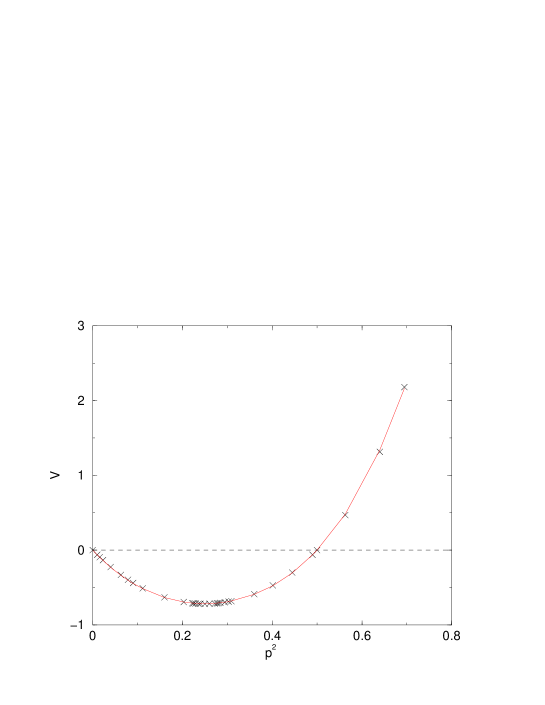
Figure 1: Graphical representation of the results

The results of this numerical procedure are depicted in table 1 for various $p^{2}$. A plot of these results is given in figure 1. There are several things to notice in this plot. The reflection symmetry around the axis $p^{2}=1/4$ seems to be most obvious. This strongly suggests an even function in $(p^{2}-1/4)$. Furthermore, the function seems to acquire its minimum at $p^{2}=1/4$ and the perturbation seems to vanish at $p^{2}=1/2$. This second observation is another strong indication for the reflection symmetry around the axis $p^{2}=1/4$ as the perturbation vanishes for $p^{2}=0$ analytically.

These observations lead us to attempt the following fit (depicted in figure 1)

$$V = -0.71775+a_{2}\;\left(p^{2}-\frac{1}{4}\right)^{2}\,+\,a_{4}\;\left(p^{2}-\frac{1}{4}\right)^{4}\;.$$

This fit produces values of $a_{2}=10.045\pm 0.054$ and $a_{4}=22.940\pm 0.363$. These errors are given by the asymptotic covariance matrix. Especially in the range $0<p^{2}<\frac{1}{2}$ this fit seems to be quite accurate; for $p^{2}>1/2$ contributions of higher orders in $\left(p^{2}-\frac{1}{4}\right)^{2}$ seem to become more important.

5 Geometrical interpretation

The calculations in this article have been performed on the $\mathbb{Z}_{2}$ orbifold subvariety of K3 moduli space. In contrast to deformations with U(1) currents which describe the relations between theories on the $\mathbb{Z}_{2}$ orbifold subvariety we have calculated deformations with twistfields that deform away from this subvariety. In the geometrical picture a deformation with twistfields leads to a transition from singular orbifolds to smooth manifolds. This transition is achieved by the so-called blowing-up of the orbifold fixed point singularities [19], [20], [21]. The blowing-up of a specific fixed point in the geometrical picture corresponds to the deformation with the twistfield located at exactly this fixed point.

Blown-up orbifolds have already been studied in the context of the Landau-Ginzburg description by giving the blowing-up modes (i.e. the twistfields) a non-vanishing vacuum expectation value [22]. A strictly conformal field theoretic approach, however, is not known to the author.

6 Conclusion and outlook

In this article, we have calculated the deformation of the conformal dimension of vertex operators deforming the $\mathbb{Z}_{2}$ orbifold model with twistfields in second order perturbation theory. This was a first attempt to this kind of problem and, hence, there are still a lot of open questions to be answered. First, we hope to validate analytically some of the conjectures based on the numerical results in this article in due course. The cases of $p^{2}>1$ and of general $\mathbb{Z}_{N}$ orbifolds should be analysable by the same methods, at least to second order in perturbation theory. Higher orders, however, seem to become more difficult very quickly. And, of course, an attempt should be made to integrate these deformations to get hold on further subvarieties in moduli space. At least, this should be possible for directions in moduli space showing a high degree of symmetry.

Acknowledgements. I would like to thank my supervisor W. Nahm for suggesting this exciting topic and for many very helpful discussions. I am also grateful to K. Wendland and A. Wißkirchen for discussions and to M. Rösgen for remarks on the manuscript.

Appendix A The four point correlator of two ground state twistfields with two vertex operators

The four point correlator of two ground state twistfields with two vertex operators in the $\mathbb{Z}_{2}$ orbifold has already been calculated in [3] based on results about off-shell string amplitudes in [23], [24] and [25], but neglecting the correct zero mode contribution. However, this has then been discussed in [9] and [10]. As this correlator is the basis for our calculations, we want to present a short derivation just using basic properties of conformal field theory.

To calculate the correlation function

$$\langle\,V^{t}_{p_{1}}(w,\bar{w})\;V^{t}_{p_{2}}(v,\bar{v})\;T_{1/2}(x,\bar{x})\;T_{-1/2}(y,\bar{y})\,\rangle$$ (19)

we want to use the OPE of the vertex operators $V^{t}_{p}(z,\bar{z})$ with any U(1) current $j(z)=i\partial X$ of the underlying toroidal theory. In order to derive this OPE, we use the mode expansion of $j(z)$

$$j(z)=\sum_{n=0}^{\infty}j_{n}z^{n-1}\quad\quad\quad j_{n}\mid\!\phi\,\rangle=0\quad\forall\;n<0\;$$

and the corresponding mode expansion of the bosonic part of the holomorphic Virasoro field

$${\cal T}_{bosonic}=\sum_{i=1}^{d}:j_{i}\;j_{i}:(z)\;.$$

Therefore, applying the Virasoro modes to the state $\mid\!V^{t}_{p}\,\rangle$, which corresponds to the vertex operator $V^{t}_{p}(0,0)$, the mode expansions give

$$\mid\!\partial V^{t}_{p}\,\rangle = L_{1}\mid\!V^{t}_{p}\,\rangle$$

$$= \frac{1}{2}(j_{0\,a}\;j_{1}^{a}+j_{1\,a}\;j_{0}^{a})\mid\!V^{t}_{p}\,\rangle$$

$$= p_{a}j_{1}^{a}\mid\!V^{t}_{p}\,\rangle\;.$$

The summations run over all d holomorphic currents in a real–d dimensional theory. This leads to the OPE

$$p_{a}j^{a}(z)\;V^{t}_{p}(w)=\frac{p^{2}}{z-w}\;V^{t}_{p}(w)+\partial_{w}V^{t}_{p}(w)+O(z-w)\;.$$ (20)

Also define the scalar product $p_{1\,a}\;p_{2}^{a}=p_{1}.p_{2}$, $p_{1}^{2}=p_{1}.p_{1}$ for the charge vectors w.r.t. to the holomorphic U(1) currents. Our goal is to find a first order differential equation for $(\ref{ver-korr})$. To achieve this we turn to the following five point correlator

$$\!\!\!\!\!\!\!\!\!\!\!\!\!\!\!\sqrt{(z-x)(z-y)}\;\langle\,p_{1a}j^{a}(z)\;V^{t}_{p_{1}}(w,\bar{w})\;V^{t}_{p_{2}}(v,\bar{v})\;T_{1/2}(x,\bar{x})\;T_{-1/2}(y,\bar{y})\,\rangle=$$ (21)

$$= \left(\sqrt{(w-x)(w-y)}\;\frac{p_{1}^{2}}{z-w}+\sqrt{(v-x)(v-y)}\;\frac{p_{1}.p_{2}}{z-v}\right)$$

$$\times\langle\,V^{t}_{p_{1}}(w,\bar{w})\;V^{t}_{p_{2}}(v,\bar{v})\;T_{1/2}(x,\bar{x})\;T_{-1/2}(y,\bar{y})\,\rangle\;.$$

This identity is justified by noticing that the square root on the left hand side of $(\ref{fuenf})$ just cancels the branching behaviour of the current $j(z)$ around the twistfields $T_{\pm 1/2}$. Hence, we have a meromorphic function in $z$ on the right hand side. The meromorphic behaviour of this right hand side is completely determined by the singular behaviour of the OPE between the current and the two vertex operators and the fact that every U(1) current drops off as $1/z^{2}$ at infinity. The behaviour with respect to the other coordinates is already contained in the four point correlator $(\ref{ver-korr})$.

Now we are ready to calculate the derivatives of $(\ref{ver-korr})$ with respect to $w$ and $v$ using the above OPE $(\ref{auch})$ and the identity $(\ref{fuenf})$

$$\partial_{w}\langle\,V^{t}_{p_{1}}(w,\bar{w})\;V^{t}_{p_{2}}(v,\bar{v})\;T_{1/2}(x,\bar{x})\;T_{-1/2}(y,\bar{y})\,\rangle=$$

$$= \lim_{z\rightarrow w}\bigg{[}\langle\,p_{1a}j^{a}(z)\;V^{t}_{p_{1}}(w,\bar{w})\;V^{t}_{p_{2}}(v,\bar{v})\;T_{1/2}(x,\bar{x})\;T_{-1/2}(y,\bar{y})\,\rangle$$

$$-\frac{p_{1}^{2}}{z-w}\langle\,V^{t}_{p_{1}}(w,\bar{w})\;V^{t}_{p_{2}}(v,\bar{v})\;T_{1/2}(x,\bar{x})\;T_{-1/2}(y,\bar{y})\,\rangle\bigg{]}$$

$$= \lim_{z\rightarrow w}\left[\left(\frac{(w-x)^{1/2}(w-y)^{1/2}}{(z-x)^{1/2}(z-y)^{1/2}}\;\frac{p_{1}^{2}}{z-w}+\frac{(v-x)^{1/2}(v-y)^{1/2}}{(z-x)^{1/2}(z-y)^{1/2}}\;\frac{p_{1}p_{2}}{z-v}\right)-\frac{p_{1}^{2}}{z-w}\right]$$

$$\times\langle\,V^{t}_{p_{1}}(w,\bar{w})\;V^{t}_{p_{2}}(v,\bar{v})\;T_{1/2}(x,\bar{x})\;T_{-1/2}(y,\bar{y})\,\rangle$$

$$= \left[\frac{-p_{1}^{2}}{2}\left(\frac{1}{w-x}+\frac{1}{w-y}\right)+\frac{p_{1}p_{2}}{w-v}\frac{(v-x)^{1/2}(v-y)^{1/2}}{(w-x)^{1/2}(w-y)^{1/2}}\right]$$

$$\times\langle\,V^{t}_{p_{1}}(w,\bar{w})\;V^{t}_{p_{2}}(v,\bar{v})\;T_{1/2}(x,\bar{x})\;T_{-1/2}(y,\bar{y})\,\rangle\;.$$

This leads to the logarithmic derivative

$$\partial_{w}\log\langle\,V^{t}_{p_{1}}(w,\bar{w})\;V^{t}_{p_{2}}(v,\bar{v})\;T_{1/2}(x,\bar{x})\;T_{-1/2}(y,\bar{y})\,\rangle=$$

$$= \frac{-p_{1}^{2}}{2}\left(\frac{1}{w-x}+\frac{1}{w-y}\right)+\frac{p_{1}p_{2}}{w-v}\frac{(v-x)^{1/2}(v-y)^{1/2}}{(w-x)^{1/2}(w-y)^{1/2}}\;.$$

Now, we define $p_{i\,l}$ to be the U(1) charge vector w.r.t. the left moving, i.e. holomorphic U(1) currents, $p_{i\,r}$ the U(1) charge vector for the right moving, i.e. antiholomorphic U(1) currents. Together with the analogous results for the derivatives with respect to $v$, $\bar{w}$ and $\bar{v}$, one gets by integration

$$\!\!\!\!\!\!\!\!\!\!\!\frac{\langle\,V^{t}_{p_{1}}(w,\bar{w})\;V^{t}_{p_{2}}(v,\bar{v})\;T_{1/2}(x,\bar{x})\;T_{-1/2}(y,\bar{y})\,\rangle}{\langle\,T_{1/2}(x,\bar{x})\;T_{-1/2}(y,\bar{y})\,\rangle}=$$ (23)

$$= c((x-y),(\bar{x}-\bar{y}))\;((w-x)(w-y))^{-p_{1l}^{2}/2}((v-x)(v-y))^{-p_{2l}^{2}/2}$$

$$\times((\bar{w}-\bar{x})(\bar{w}-\bar{y}))^{-p_{1r}^{2}/2}((\bar{v}-\bar{x})(\bar{v}-\bar{y}))^{-p_{2r}^{2}/2}$$

$$\times\left((x-y)\frac{(w-x)^{1/2}(v-y)^{1/2}+(w-y)^{1/2}(v-x)^{1/2}}{(w-x)^{1/2}(v-y)^{1/2}-(w-y)^{1/2}(v-x)^{1/2}}\right)^{-p_{1l}.p_{2l}}$$

$$\times\left((\bar{x}-\bar{y})\frac{(\bar{w}-\bar{x})^{1/2}(\bar{v}-\bar{y})^{1/2}+(\bar{w}-\bar{y})^{1/2}(\bar{v}-\bar{x})^{1/2}}{(\bar{w}-\bar{x})^{1/2}(\bar{v}-\bar{y})^{1/2}-(\bar{w}-\bar{y})^{1/2}(\bar{v}-\bar{x})^{1/2}}\right)^{-p_{1r}.p_{2r}}$$

$$= c((x-y),(\bar{x}-\bar{y}))\;((w-x)(w-y))^{-p_{1l}^{2}/2}((v-x)(v-y))^{-p_{2l}^{2}/2}$$

$$\times((\bar{w}-\bar{x})(\bar{w}-\bar{y}))^{-p_{1r}^{2}/2}((\bar{v}-\bar{x})(\bar{v}-\bar{y}))^{-p_{2r}^{2}/2}$$

$$\times\left(\frac{((w-x)^{1/2}(v-y)^{1/2}+(w-y)^{1/2}(v-x)^{1/2})^{2}}{(w-v)}\right)^{-p_{1l}.p_{2l}}$$

$$\times\left(\frac{((\bar{w}-\bar{x})^{1/2}(\bar{v}-\bar{y})^{1/2}+(\bar{w}-\bar{y})^{1/2}(\bar{v}-\bar{x})^{1/2})^{2}}{(\bar{w}-\bar{v})}\right)^{-p_{1r}.p_{2r}}\;.$$

In this article, we are only interested in the two cases $p\equiv p_{1}=\pm p_{2}$. For the case $p\equiv p_{1}=-p_{2}$ the correlator has to behave as the OPE of two vertex operators in the limit $w\rightarrow v$, i.e. as $(w-v)^{-p^{2}}$. This fixes the coefficient to

$$c_{-}((x-y),(\bar{x}-\bar{y}))=4^{-p_{r}^{2}-p_{l}^{2}}\;.$$

For the second relevant case $p\equiv p_{1}=p_{2}$, one fixes the coefficient by continuation of the correlation function on the two sheeted Riemannian surface to

$$c_{+}((x-y),(\bar{x}-\bar{y}))=4^{-p_{r}^{2}-p_{l}^{2}}\;(x-y)^{2\,p_{l}^{2}}\;(\bar{x}-\bar{y})^{2\,p_{r}^{2}}\;.$$

One can check this result by noticing that the correlator $(\ref{verkorr1})$ shows the required monodromy behaviour if one takes a vertex operator around a twistfield. This just interchanges the sign of one charge $p_{i}$.

References

[1]
M. Bershadsky and A. Radul, Conformal field theories with additional
symmetry, Int. J. Mod. Phys.A2 (1987) 165–178.
[2]
M. Bershadsky and A. Radul, G loop amplitudes in bosonic string theory in
terms of branch points, Phys. Lett.B193 (1987) 213–218.
[3]
S. Hamidi and C. Vafa, Interactions on orbifolds, Nucl. Phys.B279 (1987) 465.
[4]
L. Dixon, D. Friedan, E. Martinec, and S. Shenker, The conformal field
theory of orbifolds, Nucl. Phys.B282 (1987) 13–73.
[5]
L. J. Dixon, Some world sheet properties of superstring compactifications,
on orbifolds and otherwise, in Lectures given at the 1987 ICTP Summer
Workshop in High Energy Phsyics and Cosmology, ICTP Trieste, 1987.
[6]
A. B. Zamolodchikov, Conformal scalar field on the hyperelliptic curve and
critical Ashkin-Teller multipoint correlation functions, Nucl.
Phys.B285 (1987) 481–503.
[7]
J. J. Atick, L. J. Dixon, P. A. Griffin, and D. Nemeschansky, Multiloop
twist field correlation functions for orbifolds, Nucl. Phys.B298 (1988) 1–35.
[8]
T. T. Burwick, R. K. Kaiser, and H. F. Müller, General Yukawa
couplings of strings on orbifolds, Nucl. Phys.B355
(1991) 689–711.
[9]
J. Erler, D. Jungnickel, J. Lauer, and J. Mas, String emission from
twisted sectors: cocycle operators and modular background symmetries, Ann. Phys.217 (1992) 318–363.
[10]
D. Jungnickel, Correlation functions of two-dimensional twisted conformal
field theories.
PhD thesis, Max-Planck-Institut für Physik, München, 1992.
[11]
W. Nahm and K. Wendland, A hiker’s guide to K3: Aspects of N = (4,4)
superconformal field theory with central charge , Commun.
Math. Phys.216 (2001) 85–138,
[hep-th/9912067].
[12]
K. Wendland, Moduli Spaces of Unitary Conformal Field Theories.
PhD thesis, University of Bonn, Bonn, 2000.
[13]
L. P. Kadanoff, Multicritical behavior at the Kosterlitz-Thouless
critical point, Ann. Physics120 (1978) 39–71.
[14]
L. Kadanoff and A. Brown, Correlation functions on the critical lines of
the Baxter and Ashkin-Teller models, Ann.Physics121 (1979)
318–342.
[15]
B. R. Greene, String theory on Calabi-Yau manifolds, in Lectures
given at Theoretical Advanced Study Institute in Elementary Particle Physics
(TASI 96): Fields, Strings, and Duality, TASI 96, Boulder CO, 1996.
hep-th/9702155.
[16]
J. Polchinski, String Theory.
Cambridge University Press, Cambridge, 1998.
[17]
M. R. Gaberdiel, An introduction to conformal field theory, Rept.
Prog. Phys.63 (2000) 607,
[hep-th/9910156].
[18]
J. C. Collins, Renormalization. An Introduction to Renormalization, the
Renormalization Group, and the Operator Product Expansion.
Cambridge University Press, Cambridge, UK, 1984.
[19]
L. Dixon, J. A. Harvey, C. Vafa, and E. Witten, Strings on orbifolds,
Nucl. Phys.B261 (1985) 678–686.
[20]
P. S. Aspinwall, Resolution of orbifold singularities in string theory,
in Mirror symmetry II (S. B. Greene, S.T. Yau, ed.), pp. 355–379,
1994.
hep-th/9403123.
[21]
P. S. Aspinwall, K3 surfaces and string duality, in Differential
geometry inspired by string theory (S. Yau, ed.), 1996.
hep-th/9611137.
[22]
M. Cvetic, Blown - up orbifolds, in Superstrings, cosmology and
composite structures: proceedings (S. G. Jr. and R. Mohapatra, eds.),
(Singapore), p. 269, World Scientific, 1987.
[23]
J. H. Schwarz and C. C. Wu, Off mass shell dual amplitudes. 2, Nucl. Phys.B72 (1974) 397.
[24]
E. Corrigan and D. B. Fairlie, Off-shell states in dual resonance theory,
Nucl. Phys.B91 (1975) 527.
[25]
M. B. Green, Locality and currents for the dual string, Nucl.
Phys.B103 (1976) 333.