SU-ITP 01-03

hep-th/0103012

Fundamentals on the Noncommutative Plane

Yonatan Zunger^† Department of Physics

Stanford University

Stanford, CA 94305-4060

We consider the addition of charged matter (“fundametals”) to noncommutative Yang-Mills theory and noncommutative QED, derive Feynman rules and tree-level potentials for them, and study the divergence structure of the theory. These particles behave very much as they do in the commutative theory, except that (1) they occupy bound-state wavefunctions which are essentially those of charged particles in magnetic fields, and (2) there is slight momentum nonconservation at vertices. There is no reduction in the degree of divergence of charged fermion loops like that which affects nonplanar noncommutative Yang-Mills diagrams.

$\phantom{1}{}^{\dagger}$zunger@itp.stanford.edu

The dynamics of dipoles in two dimensions in a strong background magnetic field is governed by noncommutative Yang-Mills, (NCYM) [1, 2, 3, 4] where the dipoles are described by the gauge fields which have a noncommutative multiplication rule. This rule is equivalent to replacing the coordinate functions $x$ and $y$ with operators that have certain commutation relations, and writing the gauge fields as Taylor series in these operators. [5] Thus the gauge fields are operator-valued quantities.

Given a set of operator-valued fields, it is natural to ask what the fields are which would correspond to column vectors. In this paper we will introduce such fields, called “fundamentals” since they carry the fundamental representation of the operator algebra, and study their dynamics. We will work out Feynman rules, study some basic processes such as their 1-loop mass renormalization and their Coulomb potential, and examine the divergence structure of their theory.

Of course, such fields would not be worth studying if they did not occur in a physics context. Fortunately they are easy to come across. We will begin by setting up the problem of a charged particle in a magnetic field in the traditional quantum way, and show that the gauge field emerges as an operator-valued quantity (in the usual way) and that these fundamental fields naturally emerge as the description of the individual charged particles. It is therefore natural to suspect that in more complicated systems governed by noncommutative Yang-Mills theory (NCYM) these fields will show up as the basic kind of charged matter. More recently such fields emerged in the study of noncommutative Chern-Simons theory in 2-dimensional systems with boundary; [6] there these fields were the boundary excitations of the theory. Such theories are potentially very interesting as simple examples of holographic systems, and so their boundary fields merit particular interest.

1 Introduction: Noncommutative Geometry and Fundamentals

Consider a charged nonrelativistic particle moving on a plane in an applied constant magnetic field perpendicular to the plane. This system satisfies the Schrödinger equation $H\left|\psi\right>=i\hbar\partial_{0}\left|\psi\right>$ with Hamiltonian

$$H=\frac{1}{2m}\left(p-gA\right)^{2}$$ (1.1)

where $A=\frac{1}{2}B(-y,x)$. Later on we will allow $A$ to fluctuate about this value. This Hamiltonian really has two kinds of fields in it: Hilbert-space-valued (“fundamental”) fields such as the wave function, and operator-valued fields such as the vector potential. In a moment we will make a change of variables which will simplify this Hamiltonian at the expense of replacing the coordinates $x$ with noncommuting coordinates $\tilde{x}$. The operator-valued fields such as $A$ become functions of these noncommuting coordinates, and their dynamics is fairly well-understood. Our objective here is to study how the Hilbert space-valued fields behave both in this system and in the broader context of noncommutative Yang-Mills theory. Following the terminology from the mathematical literature, we refer to these as fundamental fields. This name comes from the fact that if one writes operators as matrices they carry two indices, while these fields carry a single index; more technically, these fields carry the fundamental representation of the algebra of functions on the space.

The change of variables is as follows. The quantity in the parentheses of (1.1) is defined to be the canonical momentum $\tilde{p}$. It obeys

$$\left[\tilde{p}_{x},\tilde{p}_{y}\right]=\left[p_{x}+\frac{1}{2}gBy,p_{y}-\frac{1}{2}gBx\right]=igB\ .$$ (1.2)

We can define coordinates which are conjugate to these momenta in the sense that $[\tilde{x}^{i},\tilde{p}_{j}]=\delta^{i}_{j}$. This is satisfied by

$$\tilde{x} = -\frac{1}{gB}\tilde{p}_{y}$$

$$\tilde{y} = \frac{1}{gB}\tilde{p}_{x}\ .$$ (1.3)

However, these coordinates do not commute with one another; they satisfy

$$[\tilde{x}^{i},\tilde{x}^{j}]=\epsilon^{ij}\frac{i}{gB}\equiv i\theta^{ij}\ .$$ (1.4)

One should be aware at this point that the commutative limit of this theory is not $\theta\rightarrow 0$ but $\theta\rightarrow\infty$. This is clear if one substitutes into (1.1), since then the $\tilde{p}$’s turn back into commuting $p$’s. The Schrödinger equation for this Hamiltonian is

$$H\left|\psi\right>=\frac{1}{2m}\left(\tilde{p}_{x}^{2}+\tilde{p}_{y}^{2}\right)\left|\psi\right>=\frac{1}{2m}\left(\tilde{p}_{x}^{2}+\theta^{-2}\tilde{x}^{2}\right)\left|\psi\right>=E\left|\psi\right>$$ (1.5)

and its solutions are 1D simple harmonic oscillator wave functions; but in the limit $\theta\rightarrow\infty$ the eigenfunctions become degenerate and can be brought by a change of basis back to 2D planewaves, which are the solutions of the original equation (1.1) at infinite $\theta$.

The potentially confusing equation in the commutative limit is (1.4). This equation is not disastrous simply because $\tilde{x}$ and $\tilde{y}$ do not have smooth limits as $\theta\rightarrow\infty$; they both diverge linearly. In this limit those are simply no longer good coordinates. One could, of course, make a change to a different set of coordinates where $\tilde{x}$ and $\tilde{y}$ remain healthy in this limit (and their commutator goes to zero) but in this case their conjugate momenta will diverge.

Given this set of “coordinate” operators, we can verify that they indeed behave somewhat like ordinary coordinates on a space by defining derivatives with respect to them. We use the canonical formula

$$D_{i}=i\tilde{p}_{i}=i\theta^{-1}_{ij}\tilde{x}^{j}$$ (1.6)

$D_{i}$ generates derivatives on states in the Hilbert space by multiplication and on operators by commutation. The first statement means that for $\left|x\right>$ an eigenket of $\tilde{x}$ and $dx$ infinitesimal,

$$\tilde{x}\left(1+dxD_{x}\right)\left|x\right>=x+dx(1+D_{x}\tilde{x})\left|x\right>=(x+dx)(1+dxD_{x})\left|x\right>\ ,$$ (1.7)

which implies that $(1+dxD_{x})\left|x\right>=\left|x+dx\right>$, so

$$D\left|x\right>=\lim_{\Delta x\rightarrow 0}\frac{\left|x+\Delta x\right>-\left|x\right>}{\Delta x}\ .$$ (1.8)

(This is just the usual proof that momenta generate translations) The second statement follows from

$$[D_{i},\tilde{x}^{j}]=\delta_{i}^{j}\ ,$$ (1.9)

which implies that

$$\left[D_{x},\sum a_{mn}\tilde{x}^{m}\tilde{y}^{n}\right]=\sum ma_{mn}\tilde{x}^{m-1}\tilde{y}^{n}\ ,$$ (1.10)

and the property

$$[D,AB]=[D,A]B+A[D,B]$$ (1.11)

which holds for any operators $A$ and $B$. Together these mean that $[D,\cdot]$ takes the derivative of any locally polynomial function of the $\tilde{x}^{i}$ in the normal manner.

It may appear strange at first glance to say that $D$ acts on operators by conjugation, since one typically writes operators as acting on one another by matrix multiplication. What this statement really means is that for any operator $A$ and any ket $\left|\psi\right>$,

$$DA\left|\psi\right>=[D,A]\left|\psi\right>+AD\left|\psi\right>$$ (1.12)

which is the product rule for an operator and a ket.

The combination of an algebra of operators (the set of operator-valued functions and their multiplication law), a Hilbert space and a derivative operator is the definition in algebraic geometry of a noncommutative space. In the commutative limit, the algebra of operators turns into the algebra of functions on the space, while the Hilbert space turns into the vector space of $L^{2}$ functions.

This notion of noncommutative space is very closely related to the one that is commonly seen in the physics literature. Typically noncommutative field theories are defined by taking ordinary field theories and replacing the product of two fields with the star product

$$f(x)\star g(x)=\left.e^{-\frac{i}{2}\theta^{ij}\frac{\partial}{\partial y^{i}}\frac{\partial}{\partial z^{j}}}f(y)g(z)\right|_{y=z=x}\ .$$ (1.13)

This star product is exactly the multiplication rule one obtains from taking the Taylor expansions of $f$ and $g$ and replacing the coordinates $x$ and $y$ with the noncommuting coordinates $\tilde{x}$ and $\tilde{y}$ above:

$$f(x)=\sum a_{mn}x^{m}y^{n}\longrightarrow\sum a_{mn}W(\tilde{x}^{m},\tilde{y}^{n})$$ (1.14)

where $W(\tilde{x}^{m},\tilde{y}^{n})$ represents the Weyl-ordered product of the operators.

We have gone through this somewhat more circuitous operator-based derivation of noncommutative theories since it highlights the presence of fundamental fields and simultaneously makes it clear what needs to be done in order to integrate them into noncommutative field theories. We wish to look at these fields as models of particles charged under noncommutative QED or YM.

Before plunging into this subject, it is useful to look briefly at theories of operator-valued fields. The theory of greatest interest to us is noncommutative QED, which follows from taking the ordinary QED Lagrangian in our background:

$${\cal L}=\frac{1}{4}F_{\mu\nu}F^{\mu\nu}$$ (1.15)

where $\mu,\nu=0,1,2$ and

$$F_{\mu\nu}=\frac{1}{ig}\left[\partial_{\mu}-igA^{0}_{\mu}-igA_{\mu},\partial_{\nu}-igA^{0}_{\nu}-igA_{\nu}\right]\ .$$ (1.16)

$A^{0}_{\mu}$ is the background vector potential $A$ of (1.1), and the $\partial_{\mu}$ are ordinary partial derivatives. But writing these derivatives in terms of momenta, we can clearly combine them with the $A^{0}$ to form our $\tilde{p}_{\mu}$. (Since $A^{0}_{0}=0$, $\tilde{p}_{0}=p_{0}$ and the time components are unchanged) Therefore we can rewrite the field strength as

$$F_{\mu\nu}=\frac{1}{ig}\left[D_{\mu}-igA_{\mu},D_{\nu}-igA_{\nu}\right]\ .$$ (1.17)

As we noted above, this is exactly the field strength one would get if one replaced multiplication with the star product in (1.15). The resulting field theory is noncommutative Yang-Mills.

One point about the solution to this theory, which will be useful later, is that the eigenfunctions of a free boson (the solutions to the Klein-Gordon equation) are essentially the same in noncommutative space and commutative space. The equation is

$$\partial_{0}^{2}A_{\mu}-\delta^{ij}[D_{i},[D_{j},A_{\mu}]]=0$$ (1.18)

and by writing $A_{\mu}$ as a Taylor series in the $\tilde{x}$ one easily verifies that the solutions are

$$A_{\mu}=e^{i(\omega t-q\cdot\hat{x})}$$ (1.19)

where $\omega^{2}-q^{2}=0$.

We now turn to our main subject of interest, the fundamental fields which are minimally coupled to the gauge fields of NCYM. Because both of the cases of physical interest to us (the particle in the magnetic field and string endings on a brane) have spin $1/2$, we will spend most of our time examining solutions of the Dirac equation

$$\left(i\not\partial+m\right)\left|\psi\right>=0\ .$$ (1.20)

There are some technical subtleties with the case of finite mass, since in a non-Lorentz-invariant theory (Lorentz-invariance is broken by the magnetic field) these fermions will lead to the violation of Ward identities and possible sicknesses in the theory at higher loops. As such we will begin our analysis by considering the limit where there are no kinetic terms in the Lagrangian. ($m=\infty$, the extreme nonrelativistic limit) This will allow us to study some simple effects like electron mass renormalization and the Coulomb force. At the end of this paper we will discuss the divergence structure of the theory, and at that point it will be at least formally interesting to restore the space derivatives in (1.20). We will do this, although we reserve judgement on the physical relevance of such solutions.

2 The Dirac action in the nonrelativistic limit

For the remainder of this paper, we will look exclusively at the properties of systems in noncommutative space, so where there is no risk of confusion we will drop tildes on the $x$’s and the $p$’s and replace $D$ with $\partial$.

We would like to write the Dirac action for Hilbert space-valued fermions in noncommutative space. If space satisfies

$$[x^{i},x^{j}]=i\theta^{ij}=i\theta\epsilon^{ij}$$ (2.21)

where $i,j$ are space indices and $\theta$ is a real number, then space derivatives are given by

$$\partial_{i}=i\theta^{-1}_{ij}x^{j}\ .$$ (2.22)

Time derivatives are unchanged from the commutative case. This means that the Laplacian operator is

$$\nabla^{2}\sim\partial_{0}^{2}+\theta^{-2}x^{2}$$ (2.23)

which is not Lorentz-invariant.

For the reasons discussed above, we will consider states that have no space derivatives on them, and so write an action

$$S=\int dtd^{2}x\bar{\psi}\left(i\gamma^{0}\nabla_{0}+m\right)\psi+L_{YM}\ .$$ (2.24)

$\nabla$ here is a gauge-covariant derivative coupling to an electromagnetic field:

$$\nabla=\partial-igA\ .$$ (2.25)

This action has a gauge symmetry $\psi\rightarrow(1+i\alpha)\psi$, $A^{\mu}\rightarrow A^{\mu}-\nabla^{\mu}\alpha$, where $\alpha$ is an infinitesimal operator-valued quantity.

We first get the fermion propagator and eigenstates by solving the system when $g=0$. (No coupling constant) Then the Green’s function satisfies

$$\left(i\gamma^{0}\partial_{0}+m\right)G=i\delta(x)\Rightarrow G(k)=\frac{i}{\gamma^{0}k_{0}+m}\ .$$ (2.26)

This is our fermion propagator. The fermion eigenstates follow from solving the Dirac equation

$$\left(i\gamma^{0}\partial_{0}+m\right)\psi=0\Rightarrow\psi(t,z)=e^{\pm imt}\left(\begin{array}[]{c}\left|\psi_{\uparrow}\right>\\ \left|\psi_{\downarrow}\right>\end{array}\right)\ .$$ (2.27)

Since there is no space dependence of the Dirac equation, the $\left|\psi_{\uparrow,\downarrow}\right>$ are unconstrained and so we are free to choose any basis of square-normalizable functions for them. We will label these by $\left|n\alpha\pm\right>$, where $n$ is an index, $\alpha$ is the spin state and $\pm$ is the sign of the frequency in (2.27). (We will choose a specific basis later when we consider the full Dirac equation; for now any basis for the Hilbert space will do) The completeness relationship for these kets is

$$\sum_{n}\left|n\alpha\pm\right>\left<n\alpha^{\prime}\pm^{\prime}\right|=\delta_{\alpha\alpha^{\prime}}\delta_{\pm\pm^{\prime}}$$ (2.28)

since the $\left|\psi_{\uparrow}\right>$ and $\left|\psi_{\downarrow}\right>$ are independently arbitrary members of the Hilbert space. More generally, we can define off-shell states $\left|z_{0};n\alpha\pm\right>$ which are also labelled by a frequency $z_{0}$ which may differ from $m$. These show up in sums over intermediate states. Their completeness relationship is

$$\int\frac{dz_{0}}{2\pi}\sum_{n}\left|z_{0};n\alpha\pm\right>\left<z_{0};n\alpha^{\prime}\pm^{\prime}\right|=\delta_{\alpha\alpha^{\prime}}\delta_{\pm\pm^{\prime}}\ .$$ (2.29)

Using this basis, the electron propagator between two off-shell states is (figure 1)

$$\frac{i}{\gamma^{0}z_{0}+m}\left<n^{\prime}\alpha^{\prime}\pm\right|\left.n\alpha\pm\right>(2\pi)\delta(z^{\prime}_{0}-z_{0})=\frac{i}{\gamma^{0}z_{0}+m}(2\pi)\delta(z^{\prime}_{0}-z_{0})\delta_{nn^{\prime}}\delta_{\alpha\alpha^{\prime}}\ .$$ (2.30)

External fermion legs are associated with factors of the on-shell fermion wave function $\left|n\alpha\pm\right>$ times $\sqrt{2m}$. (This factor is for consistency with standard normalizations in field theory)

Figure 1: The electron propagator

Figure 2: The electron-photon vertex

Finally, let $g\not=0$ and let us find the electron-photon vertex. This follows most easily from taking the variation of the action using the usual LSZ formulation, but it is instructive to get it from time-dependent perturbation theory as well. We apply a time-dependent field

$$A^{0}=\eta(t)e^{-i(u_{1}x_{1}+u_{2}x_{2})}\equiv\eta(t)G(u)$$ (2.31)

where $x_{1,2}$ are the coordinates of the noncommutative plane and $u_{1,2}$ are $c$-numbers. The perturbation in the Hamiltonian is simply $\Delta H=gA^{0}$ (from minimal coupling in the nonrelativistic theory; that’s ok because since there are no space derivatives we are essentially always working in the nonrelativistic limit) Then from ordinary perturbation theory we get

$$\psi(n,t)=\sum_{m}\frac{1}{m!}\left(\frac{-ig}{\hbar}\int dt\eta(t)\right)^{m}\sum_{n_{1}\cdots n_{m-1}}\left<n\right|G(u)\left|n_{1}\right>\left<n_{1}\right|G(u)\left|n_{2}\right>\cdots\left<n_{m-1}\right|G(u)\left|n_{0}\right>$$ (2.32)

if the particle is initially in the state $\left|n_{0}\right>$. This corresponds to an insertion of $-ig$ at each vertex, which is the same as the result which one finds from varying the Lagrangian. However, the momentum-conserving delta function which usually comes from the inner product is changed due to factors of $G(u)$. The combined vertex (including momentum factors) is thus

$$-ig(2\pi)\delta(z^{\prime}_{0}-z_{0}-u_{0})\left<z^{\prime}_{0};n^{\prime}\alpha^{\prime}\pm\right|G(u)\left|z_{0};n\alpha\pm\right>\ .$$ (2.33)

The matrix element in (2.33) can most interestingly be evaluated if we expand the fermion states in the (nonorthonormal) momentum basis

$$\left|z\right>=e^{-iz\cdot x}\left|0\right>=e^{-i\sqrt{\frac{\theta}{2}}\left(za+z^{\star}a^{\dagger}\right)}\left|0\right>=G(z)\left|0\right>$$ (2.34)

where the $a$ and $a^{\dagger}$ are SHO ladder operators normalized such that $[a,a^{\dagger}]=1$:

$$a=\frac{1}{\sqrt{2\theta}}(x^{1}-ix^{2})\ ,$$ (2.35)

so that

$$\left|n\alpha\pm\right>=\int d^{2}zu_{n\alpha\pm}(z)\left|z\right>\ .$$ (2.36)

Then the fermion-photon vertex between fermions in momentum eigenstates $z$ and $z^{\prime}$ is given by

$$-ig(2\pi)\delta(z^{\prime}_{0}-z_{0}-u_{0})f_{1}(z,z^{\prime};u)\delta_{\alpha\alpha^{\prime}}$$ (2.37)

where

$$f_{1}(z,z^{\prime};u)=\left<z^{\prime}\right|G(u)\left|z\right>=\left<0\right|G(-z^{\prime})G(u)G(z)\left|0\right>\ .$$ (2.38)

This function can be evaluated using the Baker-Hausdorff lemma and (2.34) to be

$$f_{1}(z,z^{\prime};u)=e^{-\frac{\theta}{4}\left(|q|^{2}-\left(q^{\star}z^{\prime}-qz^{\prime\star}\right)-\left(u^{\star}z+uz^{\star}\right)\right)}$$ (2.39)

where $q=z+u-z^{\prime}$ is the momentum nonconservation (“wobble”) at the vertex. Note that nonconservation is Gaussian damped and vanishes in the commutative limit; as $\theta\rightarrow\infty$ this function approaches $\delta^{2}(z^{\prime}-z-u)$, justifying the interpretation of $z$ as a space momentum. These phases are the analogue for fundamentals of the phase factors $\exp[i\sum_{i<j}p_{i}\wedge p_{j}]$ which occur at gauge boson vertices in NCYM. [3]

The momentum nonconservation follows from the fact that momenta along different directions do not commute, and therefore the labelling of fermion states by two components of momentum was mildly fallacious.

More generally, we can define

$$f_{n}(z,z^{\prime};p_{1},\ldots p_{n})=\left<z^{\prime}\right|G(p_{1})\cdots G(p_{n})\left|z\right>$$ (2.40)

which can be easily evaluated using the Baker-Hausdorff lemma. That tells us that

$$\left<0\right|G(p_{1})\cdots G(p_{N})\left|0\right>=e^{-\frac{\theta}{4}|q|^{2}}e^{i\sum_{j<i}p_{i}\wedge p_{j}}$$ (2.41)

where $q=\sum p_{i}$ and $p_{1}\wedge p_{2}=\frac{1}{2}\theta_{\mu\nu}p_{1}^{\mu}p_{2}^{\nu}$, (The factor of $2$ in the wedge product comes from our having defined $[x^{i},x^{j}]=i\theta^{ij}$, which differs by this factor of 2 from that used in some other papers) and so

$$f_{n}(z,z^{\prime};p_{1},\ldots p_{n})=e^{-\frac{\theta}{4}|q+z-z^{\prime}|^{2}}e^{i\left(\sum_{j<i}p_{i}\wedge p_{j}+(z+z^{\prime})\wedge q-z\wedge z^{\prime}\right)}\ .$$ (2.42)

This function will be useful in the calculation of general Feynman diagrams later.

One should note, though, that we did not Fourier transform anywhere to cause the space components of $z$ to behave as momenta, whereas we did do so for the time component in solving the Dirac equation. This means that integrals over momenta in loops have measure $d^{3}z/2\pi$, rather than $(2\pi)^{3}$. This corresponds with the absence of a $(2\pi)^{2}$ in the $\theta\rightarrow\infty$ limit of $f_{1}$.

The remaining Feynman rules of the theory are simply those of noncommutative Yang-Mills theory. One should note that only the zero component of the gauge field couples to the fermions.

3 The fermion two-point function

The one-loop contribution to the fermion two-point function is given in figure (3).

Using the Feynman rules above, the correction to the propagator is given by

$$(-ig)^{2}\int\frac{d^{3}udw_{0}}{(2\pi)^{4}}\sum_{m\beta}\left<z^{\prime}_{0};n^{\prime}\alpha^{\prime}\pm\right|G(-u)\left|w_{0};m\beta\pm\right>\frac{i}{\gamma^{0}w_{0}+m}\frac{ig_{00}}{u^{2}-\mu^{2}}\left<w_{0};m\beta\pm\right|G(u)\left|z_{0};n\alpha\pm\right>$$ (3.43)

where $\mu$ is a photon mass introduced as an infrared regulator. We can perform the $m\beta$ sum immediately, since they do not appear in any propagators;

$$\sum_{m\beta}\left<z^{\prime}_{0};n^{\prime}\alpha^{\prime}\pm\right|G(-u)\left|w_{0};m\beta\pm\right>\left<w_{0};m\beta\pm\right|G(u)\left|z_{0};n\alpha\pm\right> = \left<z^{\prime}_{0};n^{\prime}\alpha^{\prime}\pm\right|G(-u)G(u)\left|z_{0};n\alpha\pm\right>$$ (3.44)

$$= \left<z^{\prime}_{0};n^{\prime}\alpha^{\prime}\pm\right|\left.z_{0};n\alpha\pm\right>$$

$$= (2\pi)\delta(z^{\prime}_{0}-z_{0})\delta_{nn^{\prime}}\delta_{\alpha\alpha^{\prime}}$$

so the two-point function is

$$(-ig)^{2}\int\frac{d^{3}u}{(2\pi)^{3}}\frac{i}{\gamma^{0}(z_{0}-u_{0})+m}\frac{ig_{00}}{u^{2}-\mu^{2}}\delta(z^{\prime}_{0}-z_{0})\delta_{nn^{\prime}}\delta_{\alpha\alpha^{\prime}}$$ (3.45)

This is exactly the commutative result, except for the absence of space momenta in the fermion denominator. (Corresponding to the nonrelativistic limit we have taken)

Therefore due to a fortuitous cancellation the effects of noncommutativity – and specifically, the smearing of momentum conservation – cancels out of this diagram. This is our first example of the insensitivity of fermion properties to the value of $\theta$.

Incidentally, the integral above can be performed; using a hard cutoff $\Lambda$ to regulate momenta in the UV gives

$$\frac{g^{2}}{4\pi}\int_{\mu}^{\Lambda}du\frac{1}{z_{0}-u+m}\log\left.\frac{u^{2}+\mu^{2}}{u^{2}-\Lambda^{2}+\mu^{2}}\right|_{\mu\rightarrow 0}\ .$$ (3.46)

This is the same as the two-point function in the commutative nonrelativistic theory, and still has the characteristic log divergence.

4 Scattering and the Two-Body Hamiltonian

One simple process where we can see a nontrivial effect of momentum smearing is in the scattering of two electrons off each other.

The amplitude is (n.b. we are using a mostly negative metric)

$$iM = (-ig)^{2}\int\frac{d^{3}u}{2\pi}\bar{u}(z)f_{1}(z,z^{\prime};u)u(z)\frac{i}{u^{2}}\bar{u}(w)f_{1}(w^{\prime},w;-u)u(w^{\prime})$$ (4.47)

$$= -2img^{2}\delta(z^{\prime}_{0}+w^{\prime}_{0}-z_{0}-w_{0})\int d^{2}u\frac{\left<z\right|G(u)\left|z^{\prime}\right>\left<w\right|G(-u)\left|w^{\prime}\right>}{u^{2}-(z^{\prime}_{0}-z_{0})^{2}}\ .$$

As $\theta\rightarrow\infty$, the expectation values in the numerator become space-momentum-conserving $\delta$-functions, and this converges to the usual result for scattering of particles in two dimensions. The different term corresponds to the uncertainty in the momentum transfer.

We can extract the effective two-body Hamiltonian from this result using the first Born approximation. Noting that the $f$’s arise from sandwiching photon momentum operators $G(u)$ between external fermion states, the total Hamiltonian is

$$H=g^{2}\int\frac{d^{2}u}{|u|^{2}}G(u)\otimes G(-u)$$ (4.48)

which acts on the direct product Hilbert space of two fermions. Since these are identical fermions, the final eigenfunctions must be antisymmetrized.

We can diagonalize this Hamiltonian in a straightforward manner. In terms of SHO ladders for the two factors of the Hilbert space, it is equal to

$$H=g^{2}\int\frac{d^{2}u}{|u|^{2}}e^{-i\sqrt{\frac{\theta}{2}}(ua+u^{\star}a^{\dagger})}e^{i\sqrt{\frac{\theta}{2}}(ub+u^{\star}b^{\dagger})}$$ (4.49)

Since $a$ and $b$ commute it is useful to define a combined ladder $A=a-b$ and write

$$H=g^{2}\int\frac{d^{2}u}{|u|^{2}}e^{-i\sqrt{\frac{\theta}{2}}(uA+u^{\star}A^{\dagger})}$$ (4.50)

Now, two pairs of commuting SHO ladders naturally suggests the Schwinger construction of angular momentum. We define the operators

$$N = a^{\dagger}a+b^{\dagger}b$$

$$Q_{z} = \frac{1}{2}(a^{\dagger}b+b^{\dagger}a)$$

$$Q_{y} = \frac{1}{2}(a^{\dagger}a-b^{\dagger}b)$$

$$Q_{x} = \frac{i}{2}(b^{\dagger}a-a^{\dagger}b)\ .$$ (4.51)

The operators $Q_{x,y,z}$ generate the algebra $SU(2)$, and all commute with the total number operator $N$. $N$ is related to the quadratic Casimir by

$$Q^{2}=\frac{1}{2}N\left(\frac{1}{2}N+1\right)\ .$$ (4.52)

The eigenstates of the paired SHO’s (which are a basis for the Hilbert space) may be decomposed into an angular-momentum basis

$$\left|jm\right>=\frac{a^{\dagger(j+m)}b^{\dagger(j-m)}}{\sqrt{(j+m)!(j-m)!}}\left|00\right>$$ (4.53)

where $\left|00\right>$ is the ground state of the SHO. These states are eigenstates of $N$ and $Q_{z}$ with eigenvalues $2j$ and $m$, respectively, and $j$ and $m$ take the usual values for angular-momentum eigenstates.

These operators are useful because the Hamiltonian commutes with both $N$ and $Q_{z}$. The easiest way to see this is to expand the exponential in a Taylor series and do the integral in polar coordinates. We introduce both upper and lower bounds $\Lambda$ and $\mu$ on the radial component of this, corresponding to UV and IR cutoffs respectively.

$$H = g^{2}\int\frac{dud\alpha}{u}e^{-iu\sqrt{\frac{\theta}{2}}(e^{-i\alpha}A^{\dagger}+e^{i\alpha}A)}$$ (4.54)

$$= g^{2}\sum_{N=0}^{\infty}\frac{1}{N!}\int d\alpha duu^{N-1}\left(-i\sqrt{\frac{\theta}{2}}\right)^{N}\left(e^{-i\alpha}A^{\dagger}+e^{i\alpha}A\right)^{N}$$

$$= g^{2}\int_{0}^{2\pi}d\alpha\left[\log\frac{\Lambda}{\mu}+\sum_{N=1}^{\infty}\sum_{M=0}^{N}\frac{1}{N\cdot N!}\left(-i\Lambda\sqrt{\frac{\theta}{2}}\right)^{N}e^{i(N-2M)\alpha}C(A^{\dagger N}A^{N-M})\right]$$

$C(A^{\dagger N}A^{N-M})$ is defined to be the sum of all permutations of $N$ $A^{\dagger}$’s and $(N-M)$ $A$’s, treating permutations which differ by swapping two identical elements as distinct. (So there are $N!$ terms) We have implicitly let $\mu\rightarrow 0$ in the $N\geq 1$ terms since there are no IR divergences there. The $\alpha$ integral then gives $2\pi\delta(2M-N)$, so

$$H=2\pi g^{2}\left[\log\frac{\Lambda}{\mu}+\sum_{N=1}^{\infty}\frac{1}{2N(2N)!}\left(-\frac{\Lambda^{2}\theta}{2}\right)^{N}C(A^{\dagger N}A^{N})\right]\ .$$ (4.55)

Now, the $C$ term can be reordered using the commutation relation $[A,A^{\dagger}]=2$ into a polynomial in $A^{\dagger}A$. The precise form of this polynomial is messy and involves a good deal of combinatorics, but its leading term is $(2N)!(A^{\dagger}A)^{N}$. (Lower terms are subdominant at large $N$ and so become weak when $\theta\Lambda^{2}$ is large) So pulling out an overall factor of $1/2$, we find

$$H=\pi g^{2}\left[\log\frac{\Lambda^{2}}{\mu^{2}}+\sum\frac{1}{N}\left(-\frac{\Lambda^{2}\theta}{2}A^{\dagger}A\right)^{N}+corrxns.\right]$$ (4.56)

At this point one should note that, although the integral is an infinite series in $\Lambda$, it is only logarithmically divergent. This can be seen from the original integral since it is given by a phase factor divided by $u$. In fact, if one replaces $A$ and $A^{\dagger}$ in (4.50) by numbers (as they would be in matrix elements of the Hamiltonian) the integral can be done explicitly in terms of Bessel functions, and apart from the overall logarithm term the integral goes to a constant in the large-$\Lambda$ limit. The entire $\Lambda$-dependence is therefore limited to replacing $\mu$ and $\theta$ with the dimensionless quantities

$$\hat{\mu} = \frac{\mu}{\Lambda}$$

$$\hat{\theta} = \theta\Lambda^{2}\ .$$ (4.57)

If we rewrite $A^{\dagger}A$ in terms of the angular-momentum operators above, we can then resum the series and find

$$H=\pi g^{2}\left[\log\hat{\theta}\left(\frac{1}{2}N-Q_{z}\right)-\log\hat{\mu}^{2}+corrxns.\right]$$ (4.58)

The corrections are also polynomial in $A^{\dagger}A=N-2Q_{z}$ and so the Hamiltonian as a whole commutes with both $N$ and $Q_{z}$. Therefore the eigenstates are the angular momentum eigenstates, and (since all of the coefficients in $C$ are positive) the ground state is that anihilated by $N-2Q_{z}$. These states have $j=m$, and therefore correspond to all of the relative angular momentum being in the plane.

The meaning of taking $\Lambda\rightarrow\infty$ in this context is not fully clear. It seems most natural to leave $\theta$ fixed and so allow $\hat{\theta}$ to go to infinity. If one does this, then the two-fermion effective potential is insensitive to the original value of $\theta$. A second possibility is to let $\theta\rightarrow 0$ so that $\hat{\theta}$ remains fixed. This parameter is known to be an order parameter in the striping phase transition of scalar $\phi^{4}$ theory in noncommutative space, [8] and it may have relevance in this system as well.

The $\hat{\mu}$ dependence of this Hamiltonian is the ordinary IR divergence of the Coulomb potential in 2D, and represents an overall constant which is uninteresting.

4.1 A check

Excited states can also be reached by acting with $A^{\dagger}$ on a ground state. A good check on the finiteness of this whole matter (as well as on $\theta$-blindness) is to evaluate $\left<H\right>$ in such a state. The normalized states are

$$\frac{1}{\sqrt{2^{N}N!}}A^{\dagger N}\left|0\right>$$ (4.59)

and so

$$\left<H\right>=g^{2}\int\frac{d^{2}u}{|u|^{2}}\frac{1}{2^{N}N!}e^{|u|^{2}\theta/2}\left<0\right|A^{N}e^{-iuA/\sqrt{\theta/2}}e^{-iu^{\star}A^{\dagger}/\sqrt{\theta/2}}A^{\dagger N}\left|0\right>$$ (4.60)

where we have reorganized $G$ using the Baker-Hausdorff lemma. This is then

$$\left<H\right> = \frac{g^{2}}{2^{N}N!}\int\frac{d^{2}u}{|u|^{2}}\left(i\sqrt{\frac{2}{\theta}}\right)^{2N}e^{|u|^{2}\theta/2}\left(\partial^{N}\bar{\partial}^{N}\right)\left<0\right|e^{-iuA/\sqrt{\theta/2}}e^{-iu^{\star}A^{\dagger}/\sqrt{\theta/2}}\left|0\right>$$ (4.61)

$$= \frac{g^{2}}{2^{N}N!}\int\frac{d^{2}u}{|u|^{2}}e^{|u|^{2}\theta/2}\left(\partial\bar{\partial}\right)^{N}\left[e^{-|u|^{2}\theta/2}\left<0\right|G(u)\left|0\right>\right]$$

$$= \frac{g^{2}}{2^{N}N!}\int\frac{d^{2}u}{|u|^{2}}e^{|u|^{2}\theta/2}\left(\partial\bar{\partial}\right)^{N}e^{-|u|^{2}\theta}\ .$$

The evaluation of the derivatives is a simple matter of combinatorics, and the integral may be evaluated in polar coordinates as above. The result is

$$\left<H\right> = 2\pi g^{2}\sum_{m=0}^{N}\frac{N!}{(N-m)!(m!)^{2}}(-\theta)^{m}\int duu^{2m-1}e^{-|u|^{2}\theta/2}$$ (4.62)

$$= 2\pi g^{2}\left[\int\frac{du}{u}e^{-|u|^{2}\theta/2}+\sum_{m=1}^{N}\frac{(-1)^{m-1}N!}{(N-m)!m\cdot m!}\right]\ .$$

The first term is infrared divergent but is a constant which may be removed from the Hamiltonian; it is the analogue of the $\log\hat{\mu}$ term above. It is independent of $N$ and so after this removal all of the energies are finite.

5 Space momenta

In the next section, we will derive general rules for the divergence structure of NCYM with fundamental fermions analogous to the rules for planar and nonplanar graphs in pure NCYM. While we could do this now, it is interesting to generalize our considerations to systems where the fermions have space momenta, and particle-antiparticle creation is allowed. So this section describes how to add those momenta and get the general Feynman rules for the theory.

We will begin by solving the first-quantized Dirac equation for fundamental fermions with kinetic energy. The solutions will be related to SHO eigenfunctions. The major features which distinguishes these fermions from those in commutative space are lack of Lorentz-invariance and the discreteness of the solution set. Once we have these solutions, we will write down the second-quantized Lagrangian and derive Feynman rules. With a few simple manipulations, we will show that these rules are almost identical to those in the commutative theory, except that (1) fermion momentum integrals are replaced by sums over solutions to the Dirac equation, and (2) momentum-conserving $\delta$-functions will be replaced with a smeared function which includes phases. These phases will be key in our analysis of divergences in the next section.

5.1 The Dirac equation

The Dirac equation for fundamental fermions is

$$(i\not\partial+m)\psi=0\ .$$ (5.63)

Here $\psi$ is an element of the Hilbert space rather than the algebra, so $\partial$ acts on $\psi$ by multiplication rather than commutation. We pick metric $\eta=+--$ and $\gamma_{0}=\sigma_{3}$, $\gamma_{1}=i\sigma_{1}$, $\gamma_{2}=i\sigma_{2}$. We write $\psi(x,t)=e^{-i\omega t}\psi(x)$, and multiply the equation on the left by $\gamma_{0}$. Using $\partial_{i}=-i\theta^{-1}_{ij}x^{j}$ this means

$$\left(\begin{array}[]{cc}\omega+m&-\sqrt{\frac{2}{\theta}}a^{\dagger}\\ -\sqrt{\frac{2}{\theta}}a&\omega-m\end{array}\right)\psi=0$$ (5.64)

Setting the determinant equal to zero, we find that this is solved by

$$\psi=\frac{1}{\sqrt{2\omega(\omega+m)}}\left(\begin{array}[]{c}\sqrt{\frac{2n}{\theta}}\left|n\right>\\ (\omega+m)\left|n-1\right>\end{array}\right)$$ (5.65)

where

$$\omega^{2}=m^{2}+\frac{2n}{\theta}\ .$$ (5.66)

The two signs of $\omega$ correspond, as usual, to particle and antiparticle solutions, and $\left|n\right>$ are SHO eigenstates. We label these states as $\left|n\alpha\pm\right>$, where $n$ is the SHO level, $\alpha$ is the spin index, and $\pm$ is the sign of $\omega$. Off-shell solutions are characterized by other values of $\omega$.

It is again possible to write these functions as linear combinations of momentum eigenstates $\left|z\right>=G(z)\left|0\right>$, which will be useful later but which we will not do explicitly here; we will simply note that there are functions such that

$$\left|n\alpha\pm\right>=\int d^{2}zu_{n\alpha\pm}(z)\left|z\right>\ .$$ (5.67)

The second quantization of this system proceeds in the usual way. We write a fermion operator

$$\Psi=\sum_{n\alpha}a_{n\alpha}\left|n\alpha+\right>+b^{\dagger}_{n\alpha}\left|n\alpha-\right>$$ (5.68)

where $a_{n\alpha}$ and $b_{n\alpha}$ are ladder operators satisfying canonical anticommutation relations. The Hamiltonian density is

$${\cal H}=-i\gamma\cdot\nabla+m$$ (5.69)

(so that ${\cal H}\left|n\alpha\pm\right>=\pm\gamma^{0}\omega(n,\alpha)\left|n\alpha\pm\right>$), and the overall Hamiltonian is

$$H=\bar{\Psi}{\cal H}\Psi=\sum_{n\alpha}\omega(n,\alpha)\left(a^{\dagger}_{n\alpha}a_{n\alpha}+b^{\dagger}_{n\alpha}b_{n\alpha}\right)\ .$$ (5.70)

(Plus, as usual, an infinite normal ordering constant)

The interactions with the electromagnetic field come from the covariant derivative, in a term

$$L_{int}=g\bar{\Psi}\not A\Psi\ .$$ (5.71)

When we quantize $A$, we solve the Klein-Gordon equation for algebra-valued functions (rather than Hilbert-space valued functions like $\psi$) and as is well-known the solutions to that are plane-waves $G(z)=e^{-iz\cdot x}$.

5.2 Feynman rules

Instead of deriving the Feynman rules for this system in momentum space, though, we will leave most of the quantities as operators and take explicit representations only when performing diagrammatic integrals. (This will make some properties of the system more evident) Thus to a fermion propagator we associate the factor

$$\epsfbox{eprop.eps}=S_{F}=\frac{i}{i\not\partial+m}\ .$$ (5.72)

(with appropriate placement of $i\epsilon$’s to fix the poles properly) External fermion lines are associated with terms $\left|n\alpha\pm\right>$ (for incoming lines) or $\left<n\alpha\pm\right|$ (for outgoing lines.) Internal fermion loops are associated with bracketing complete expressions in $\left<n\alpha\pm\right|$ and $\left|n\alpha\pm\right>$ and summing over $(n,\alpha)$, which is simply a trace over fermion states; there is also the usual factor of $-1$ for fermion loops coming from anticommutation. The fermion-fermion-photon vertex comes from expanding $A$ in momentum states and varying the Lagrangian, giving a term

$$\epsfbox{vertex.eps}=-ig(2\pi)\delta(z^{\prime}_{0}-z_{0}-u_{0})\gamma^{\mu}_{\alpha\dot{\beta}}G(u)\ ,$$ (5.73)

where $\mu$ is the polarization of the photon, $u$ is its momentum, and $\alpha$ and $\dot{\beta}$ are the spin states of the incoming and outgoing fermion lines, respectively.

Since vertices and propagators are now operator-valued rather than number-valued, one should keep in mind the following rules for assembling them into diagrams. One associates a separate “channel” with each fermion line, which is capped at either end either by bras and kets representing the external fermion states, or by the internal states which are summed over to form a trace for internal lines. Then one adds the various relevant operators $S_{F}$ and $-ig\gamma G$ in the order in which they appear, starting from the incoming point and going to the outgoing point. In the case of internal fermion lines, it does not matter at which point one begins since the trace is cyclically symmetric.

As an example of how these rules are applied, consider the diagram in figure 3 below. The diagram has three fermionic “channels” and several photon lines. Its value is

$$i{\cal M} = \int\frac{d^{3}pd^{3}qd^{3}r}{(2\pi)^{9}}(-1)\sum_{l,\gamma}\frac{i^{3}}{q^{2}r^{2}p^{2}}\left<n^{\prime}\alpha^{\prime}+\right|(-ig\gamma^{\mu})G(-q)S_{F}(-ig\gamma^{\nu})G(-p)\left|n^{\prime}\alpha^{\prime}+\right>$$ (5.74)

$$\cdot\left<l\gamma+\right|S_{F}(-ig\gamma_{\mu})G(q)S_{F}(-ig\gamma^{\rho})G(-r)\left|l\gamma+\right>$$

$$\cdot\left<m^{\prime}\beta^{\prime}-\right|(-ig\gamma_{\rho})G(r)S_{F}(-ig\gamma_{\nu})G(p)\left|m\beta-\right>$$

Figure 3: A two-loop diagram

We can reduce these operator rules to ordinary Feynman rules by using some simple identities. First, from $[\partial_{i},G(u)]=-iu_{i}G(u)$ it follows that

$$G(u)\frac{i}{i\not\partial+m}=\frac{i}{i\not\partial+\not u+m}G(u)\ .$$ (5.75)

So consider some general Feynman diagram. It will have a photon part which is possibly very complicated, and for each fermion line it will have a term that looks like

$$\left<n^{\prime}\alpha^{\prime}\pm\right|S_{F}G(p_{1})S_{F}\cdots G(p_{N})S_{F}\left|n\alpha\pm\right>\ .$$ (5.76)

The outer states will either be fixed states (for external lines) or traced over (for internal lines). We first push all of the fermion propagators to the left, giving

$$\left<n^{\prime}\alpha^{\prime}\pm\right|\frac{i}{i\not\partial+m}\frac{i}{i\not\partial+\not p_{1}+m}\cdots\frac{i}{i\not\partial+\sum\not p_{i}+m}G(p_{1})\cdots G(p_{N})\left|n\alpha\pm\right>\ .$$ (5.77)

Now we insert a complete set of momentum eigenstates after the initial bra, expressing the state $\left|n\alpha\pm\right>$ in terms of momentum eigenstates. This gives us

$$\int dz\bar{u}_{n^{\prime}\alpha^{\prime}\pm}(z)\frac{i}{\not z+m}\cdots\frac{i}{\not z+\sum\not p_{i}+m}\left<z\right|G(p_{1})\cdots G(p_{N})\left|n\alpha\pm\right>\ .$$ (5.78)

So clearly the propagators are exactly the same as in the commutative case. The term involving the $G$’s is the analogue of the momentum-conserving $\delta$-function, which after expanding $\left|n\alpha\pm\right>$ in a momentum basis is precisely one of the $f_{n}$’s of equation (2.42).

Using these rules, the diagram of figure 3 is equal to

$$i{\cal M} = \int\frac{d^{3}pd^{3}qd^{3}r}{(2\pi)^{9}}(-1)\sum_{l,\gamma}\frac{1}{q^{2}r^{2}p^{2}}\left[\bar{u}_{n^{\prime}\alpha^{\prime}+}(z^{\prime}_{1})(-ig\gamma^{\mu})\frac{i}{\not z^{\prime}_{1}-\not q+m}(-ig\gamma^{\nu})\right.$$ (5.79)

$$\left.\frac{}{}\cdot u_{n\alpha+}(z_{1})f_{2}(z_{1},z^{\prime}_{1};-p,-q)\right]\left[\bar{u}_{l\gamma+}(z^{\prime}_{2})\frac{i}{\not z^{\prime}_{2}+m}(-ig\gamma_{\mu})\frac{i}{\not z^{\prime}_{2}+\not q+m}\right.$$

$$\left.\frac{}{}\cdot(-ig\gamma^{\rho})u_{l\gamma+}(z_{2})f_{2}(z_{2},z^{\prime}_{2};q,-r)\right]\left[\bar{u}_{m^{\prime}\beta^{\prime}-}(z^{\prime}_{3})(-ig\gamma_{\rho})\frac{i}{\not z^{\prime}_{3}+\not r+m}\right.$$

$$\left.\frac{}{}\cdot(-ig\gamma_{\nu})u_{m\beta-}(z_{3})f_{2}(z_{3},z^{\prime}_{3};p,r)\right]$$

where we have implicitly integrated over the momenta $z_{i}$. As anticipated, the only difference between this and the commutative case is the bound-state nature of the $u_{n\alpha\pm}$ and the replacement of momentum-conserving $\delta$-functions with $f_{n}$’s.

6 Divergence structure

We wish to find the divergence structure of a general NCYM diagram involving fermions. This would be the analogue of the rule that planar graphs in NCYM have only phase factors corresponding to external legs, while nonplanar graphs have phase factors inside loops and are therefore less divergent. [3] This followed from introducing a double-line notation in which lines are associated with their phase factors, and noting that changes in the diagram which preserve planarity leave all of these factors invariant. One could then rearrange the diagrams into a tree (out of which external lines may come), a sequence of tadpoles, and a nonplanar region. The phase factors from the tree and the tadpoles all cancel out except for some overall factors on the outer legs, whereas the phase factors in the nonplanar region cause all loop integrals resulting therefrom to be strongly damped. The resulting integrals can be evaluated and contains both the divergences familiar from the commutative theory and some terms specific to noncommutative Yang-Mills. [9, 10, 11] We would like to extend this argument to add single-line diagrams corresponding to fundamentals. We will see that the rule for fermions is that they never contribute additional internal phase factors; in fact, at the level of double-line diagrams their influence can always be replicated by certain planar networks (trees) of gauge fields.

The argument is as follows. We first consider the issue of momentum nonconservation. If in any subdiagram of a given diagram the wobble ($q+z-z^{\prime}$ in (2.42)) is nonzero, that diagram contains both Gaussian damping factors and phase factors containing both $q$ and fermion momenta. Therefore, the leading divergences come from terms where there is no nonconservation, and so the only effect of the $f_{n}$ is to introduce phase factors at each fermion-photon vertex.

Because this is the only remaining difference from the commutative case, from here on out we will be concerned only with phase factors and can therefore draw simplified diagrams where photons are represented by double lines, fermions by single lines, and each vertex is associated simply with its phase factor $e^{iz^{\prime}\wedge z}$. (cf. (2.39) when $q=0$) We draw shaded circles for each vertex to make their location more clear in the figures.

The procedure for evaluating phase contributions to divergences is as follows. Consider an arbitrary diagram with photon and fermion lines.

1. First, “purely internal” networks of fermions can be integrated out. These are defined as networks of fermion lines which do not include any external fermions. Since fermions can only attach at $\psi\psi\gamma$ vertices, such networks must form polygons with $N$ external photon legs. If the momenta are as shown in figure (4) below, the diagram will contain a term

   $$\int dzdz^{\prime}\left<n^{\prime}\alpha^{\prime}+\right|\left.z^{\prime}\right>\left<z\right|\left.n\alpha+\right>\exp i\left(\sum_{j<i}q_{i}\wedge q_{j}+(z+z^{\prime})\wedge\left(\sum q_{i}\right)-z\wedge z^{\prime}\right)\cdots$$ (6.80)

   $$= \int dzdz^{\prime}\left<n^{\prime}\alpha^{\prime}+\right|\left.z^{\prime}\right>\left<z\right|\left.n\alpha+\right>\exp i\left(\sum_{j<i}q_{i}\wedge q_{j}-z\wedge z^{\prime}\right)\cdots\ .$$

   since the wobble $\sum q_{i}+z-z^{\prime}=0$. This diagram is clearly most divergent when $z\wedge z^{\prime}=0$, where it becomes equal to its commutative-space value times an overall phase factor

   $$\exp i\sum_{j<i}q_{i}\wedge q_{j}\ .$$ (6.81)

   Terms with phase factors contribute only finite amounts, since the exponential phase factor can cancel any power-law divergence.

   

   
   

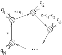
   Figure 4: An internal fermion network.

   This phase factor has two important properties. First, it does not involve the loop momentum at all, so there is no damping of this loop integral relative to the commutative theory. Thus this loop is as divergent as usual. Second, the phase factor for this effective $N$-photon vertex is exactly equal to the phase factor one would get from a planar subdiagram (a tree) of pure NCYM with $N$ external legs. We can therefore integrate out this fermion loop, with the diagram receiving whatever divergences would be appropriate in the commutative theory, and replace it with such an effective tree for the purpose of phase analysis.

2. Now we consider external fermion legs. An external fermion can attach to the rest of the diagram in one of two ways: (fig. 5)

   

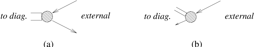
   Figure 5: External fermion attachments.

   If it attaches by (b), then there is a single fermion line entering the rest of the diagram which again must attach via either (a) or (b). This process repeats indefinitely until it is cut off by a connection of type (a). Therefore all external fermion connections must take the form of fig. 6.

   

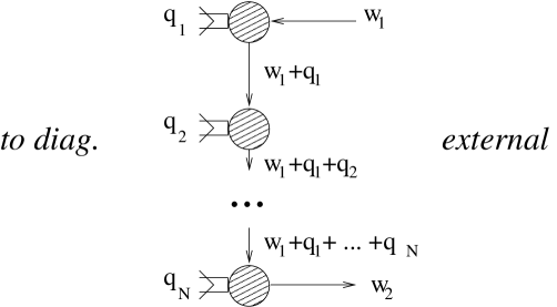
   Figure 6: All external fermion attachments must ultimately have this form.

   This is an effective $N$-photon 2-fermion vertex, whose phase may be easily calculated. Using the momentum conventions given in the figure, the phase is

   $$\phi = \exp i\left[(w_{1}+q_{1})\wedge w_{1}+(w_{1}+q_{1}+q_{2})\wedge(w_{1}+q_{1})+\cdots\right.$$ (6.82)

   $$\left.+(w_{1}+q_{1}+\cdots q_{N})\wedge(w_{1}+q_{1}+\cdots q_{N-1})\right]$$

   $$= \exp i\left[q_{1}\wedge w_{1}+q_{2}\wedge(w_{1}+q_{1})+\cdots q_{N}\wedge(w_{1}+q_{1}+\cdots q_{N-1})\right]$$

   $$= \exp i\left[w_{2}\wedge w_{1}+\sum_{j<i\leq N}q_{i}\wedge q_{j}\right]$$

   where we have used the fact that $w_{2}=w_{1}+\sum q_{i}$. But this phase is precisely the phase that would come from an $(N+1)$-photon vertex attached to a single fermion-fermion-photon vertex, so we can replace this effective vertex with precisely that. (As before, the $(N+1)$-photon vertex can then be reduced to a planar network of NCYM vertices)

3. We have therefore eliminated all internal fermion lines in favor of planar networks of NCYM vertices, and attached all external fermion lines with fermion-fermion-photon vertices where both fermions are external. It is therefore possible to now perform the ordinary channel-swapping moves of NCYM to rearrange the purely photonic part of the diagram into a tree, some tadpoles, and a nonplanar part, with some of the external photon lines now “capped” with a fermion-fermion-photon vertex. From the ordinary evaluation of divergences, we know that the nonplanar part will be suppressed by phase factors inside loops, and the divergences will be dominated by diagrams whose photonic part is purely planar. Since internal fermion lines always contribute planar NCYM effective diagrams, we find that fermions never decrease the degree of divergence in a graph.

The theory of fundamentals on the noncommutative plane is therefore a straightforward extension of ordinary NCYM theory. The behavior is not qualitatively surprising, reducing simply to the combination of bound-state wavefunctions and the momentum nonconservation which we have seen in several forms. The major open question at this point is the extent to which this can be used to construct physically interesting and realistic models of systems in strong background fields, which will hopefully further elucidate the meaning of spacetime noncommutativity in physics.

Acknowledgements

The author wishes to thank Leonard Susskind for extensive discussions and assistance on this work, especially on the subjects of sections 2 and 4. Thanks also to Nelia Mann for reading a preliminary version of this file and making numerous helpful suggestions. This work was supported by the National Science Foundation (NSF) under grant PHY-9870015.

References

- [1] N. Seiberg and E. Witten, “String theory and noncommutative geometry,” JHEP9909, 032 (1999) [hep-th/9908142].
- [2] See, e.g. L. Susskind, “The quantum Hall fluid and non-commutative Chern Simons theory,” hep-th/0101029.
- [3] D. Bigatti and L. Susskind, “Magnetic fields, branes and noncommutative geometry,” Phys. Rev. D62, 066004 (2000) [hep-th/9908056].
- [4] M. M. Sheikh-Jabbari, “Open strings in a B-field background as electric dipoles,” Phys. Lett. B 455, 129 (1999) [hep-th/9901080].
- [5] R. Gopakumar, S. Minwalla and A. Strominger, “Noncommutative solitons,” JHEP0005, 020 (2000) [hep-th/0003160].
- [6] A. P. Polychronakos, “Quantum Hall states as matrix Chern-Simons theory,” hep-th/0103013.
- [7] A. Connes, Noncommutative Geometry. Academic Press, 1994.
- [8] S. S. Gubser and S. L. Sondhi, “Phase structure of non-commutative scalar field theories,” [hep-th/0006119].
- [9] S. Minwalla, M. Van Raamsdonk and N. Seiberg, “Noncommutative perturbative dynamics,” JHEP0002, 020 (2000) [hep-th/9912072].
- [10] M. Van Raamsdonk and N. Seiberg, “Comments on noncommutative perturbative dynamics,” JHEP0003, 035 (2000) [hep-th/0002186].
- [11] M. Hayakawa, “Perturbative analysis on infrared and ultraviolet aspects of noncommutative QED on R**4,” hep-th/9912167.