Abstract

Superstring theory is the most powerful candidate for the theory unifying Standard model and gravity, and this field has been rigorously researched. The discovery of a BPS object named D-brane has lead to the idea that different kinds of superstring theory - type IIA, type IIB, type I, $SO(32)$ heterotic and $E_{8}\times E_{8}$ heterotic theory - are related with each other by duality. Now, the formulation of superstring theory has been realized only perturbatively. However, if we succeed in the formulation of the constructive definition of superstring theory, which does not depend on the perturbation, this will be a genuine unified theory describing all interactions. ’Matrix model’ is regarded as the most powerful arena to describe the nonperturbative superstring theory. Here, we mean ’matrix model’ by a model in which the theory is described in terms of $N\times N$ matrices and superstring theory is reproduced in the limit $N\to\infty$. This belief is based on the series of works in the late 1980’s. These works have provided us with the computation of the exact solution of the nonperturbative bosonic string theory in less than 1 dimensional spacetime by describing the bosonic string in terms of $N\times N$ matrices. Many proposals for the constructive definition of superstring theory have been hitherto made, and the most successful existing proposal is IKKT model. This is a dimensional reduction of 10 dimensional ${\cal N}=1$ SYM to 0 dimension, and is identical to the matrix regularization of the Green-Schwarz action of type IIB superstring theory. Yet, it is an exciting issue to pursue a model exceeding IKKT model, and we investigate the matrix model proposed by L. Smolin [13] [17]. He proposed a cubic matrix model in which both the bosons and the fermions are embedded in one multiplet. He proposed two Lie algebras for the framework of this cubic matrix model. One is $osp(1|32,R)$. This is a natural arena in that this is the maximal simple Lie algebra of the symmetry of 11 dimensional M-theory. The other is the $u(1|16,16)$, which is suggested as an extension of $osp(1|32,R)$. This paper reports the research of the formulation of the matrix model based on Smolin’s proposal. We discuss the original proposal $osp(1|32,R)$ super Lie algebra, and $gl(1|32,R)$, which is the analytic continuation of the gauged $u(1|16,16)$ theory. We discuss the relationship with the existing matrix model and the supersymmetry for these two models. This paper is based on the collaboration with S. Iso, H. Kawai and Y. Ohwashi [1].

1 Introduction

One of the main themes in elementary particle physics is unification. Four kinds of interactions are known - weak, strong, electromagnetic and gravitational interactions. Much effort has been hitherto made to understand these interactions by means of a unified quantized theory. In 1967, the Glashow-Weinberg-Salam model succeeded in unifying the electromagnetic and weak interactions in terms of $SU(2)\times U(1)$ gauge theory. The ensuing success is the emergence of Grand Unified Theory (GUT) in the early 1970’s, which further unifies the strong interactions. This theory possesses the gauge group $SU(3)\times SU(2)\times U(1)$, and another name is Standard Model.

Figure 1: The chronological table of the development of particle physics. All four interactions are believed to be unified by superstring theory.

The last and most difficult theme is the unification of the gravity. Unlike the other interactions, the gravitational interaction cannot be renormalized due to the intense divergence. Then we require another formalism than the gauge theory to complete a consistent quantum theory which unifies the Standard Model and the gravity. The most promising candidate is the superstring theory.

Superstring theory possesses many splendid properties. Superstring theory naturally contains not only matter and gauge fields but also gravitational fields. Every consistent superstring theory contains a massless spin-2 state, which corresponds to graviton. It possesses a sufficiently large gauge group to include the conventional Standard model. $E_{8}\times E_{8}$ heterotic superstring compactified on Calabi-Yau manifold is strikingly similar to the $SU(3)\times SU(2)\times U(1)$ Standard Model.

The research of superstring theory has advanced at an astonishing rate in recent years. One of the significant discovery of superstring theory is the BPS object named D-brane, defined as an object on which a superstring can terminate. D-brane has made a remarkable contribution in the unification of five kinds of superstring which seems to differ in the perturbative framework - type I, type IIA, type IIB, $SO(32)$ heterotic and $E_{8}\times E_{8}$ heterotic superstring theory. The discovery of D-brane enables us to relate these theories by duality, and these theories are now regarded as a limit of one unified theory. And if we succeed in finding the constructive definition, which describes the nonperturbative behavior of the superstring, of any one of these superstring theories, the rest of the theories are described by duality, perturbatively or nonperturbatively. If such a theory is found, this may become ’Theory of Everything’. The word ’Theory of Everything’ means the theory which describes all interactions and phenomena in our whole universe. We believe that all interactions in the whole universe are distinguished by the above-mentioned four interactions, and if we obtain a theory which unifies all of them, this can be called ’Theory of Everything’. The last and the biggest dream of particle physics is to find this ultimate theory.

Figure 2: All string theories, and M-theory, are conjectured to be a limit of one theory.

Now, many string theorists believe the conjecture that the unified theory may be described by a matrix model. The first proposal was made by Banks, Fischler, Shenker and Susskind [4]. Their matrix model was obtained by the dimensional reduction of the 10 dimensional super-Yang-Mills(SYM) theory to 1 dimension. This model are deeply related to type IIA superstring theory, and type IIA SUGRA is induced by one-loop effect. In this theory, the physical quantities are described by $N\times N$ matrices, and when we take the size of these matrices to an infinity, this theory gives a microscopic second-quantized description of M-theory in light-cone coordinates.

Another proposal for a matrix model was made by Ishibashi, Kawai, Kitazawa and Tsuchiya [5] . This is IKKT (IIB matrix) model and is the most powerful candidate for the constructive definition of superstring theory. This theory is the dimensional reduction of the 10 dimensional SYM theory to 0 dimension. The action of IKKT model is surprisingly simple :

$$S=-\frac{1}{g^{2}}Tr(\frac{1}{4}[A_{i},A_{j}][A^{i},A^{j}]+\frac{1}{2}{\bar{\psi}}\Gamma^{i}[A_{i},\psi]).$$ (1.1)

As the name of this theory indicates, this theory is deeply related to type IIB superstring theory. This theory has splendid properties, which we explain in Sec. 3. These properties gives us a confidence that IKKT model may be a successful constructive definition of the superstring theory.

Then, here comes one simple but fundamental question.

Why do we stick to the large N matrix theory ?

The background of this belief dates back to the late 1980’s , long before the discovery of D-brane by J. Polchinski. Grand Unified Theory (GUT) was a great success in unifying three of the four fundamental interactions in elementary particle physics. Another success is the description of the nonperturbative behavior of Quantum Chromodynamics(QCD). There are two ways to describe the strong-coupling region - large $N$ expansion and lattice gauge theory. It has been speculated that the same may be true of string theory, and many attempts have been made to describe string theory in terms of large $N$ matrix theory. Brezin and Kazakov [25] succeeded in solving exactly the behavior of bosonic string theory of less than 1 spacetime dimension by means of orthogonal polynomial method, and their analysis well reproduced the behavior of string theory. These works, although they do not give so many clues technically, support strongly the belief that the nonperturbative behavior of superstring theory should be described by large $N$ matrix theory.

Based on this philosophy, we speculate that the Ariadne’s thread to ’Theory of Everything’ should lie in large $N$ matrix theory. Our research is a pursuit of another matrix model than IKKT model, expecting this to exceed IKKT model, and the clue to the new matrix model was proposed by L. Smolin [13] [17]. He proposed a cubic matrix model with the multiplet belonging to super Lie algebra $osp(1|32,R)$ or $u(1|16,16)$. This super Lie algebra $osp(1|32,R)$ has been known as the maximal super Lie algebra possessing the symmetry of 11 dimensional M-theory, and this super Lie algebra is a natural arena for describing a constructive definition of superstring theory. We will explain in the subsequent section our motivation to follow the idea of L. Smolin and pursue this cubic matrix model.

This paper is organized as follows.

• Sec. 2. is devoted to a brief review of the success of old matrix theory. Although this knowledge does not provide one with the technical hint of modern matrix model, these series of works are of importance in that they give us the belief that the constructive definition of superstring theory should be described by matrix model.

• Sec. 3. is a brief review of IKKT model. We review the successful aspects of this model, and especially introduce a knowledge we inherit in our research of the new cubic matrix model.

• Sec. 4. is based on our research of $osp(1|32,R)$ cubic matrix model [1]. We especially investigate the relationship of this cubic matrix model with the existing proposal of matrix model. We compare the supersymmetry of this cubic matrix model with IKKT model, and consider how IKKT model is induced from the cubic matrix model.

• Sec. 5. introduces another version of this cubic matrix model, called ’gauged action’. We treat the theory with the gauge symmetry vastly enhanced, following the idea of L. Smolin [17]. The multiplets now belong to $gl(1|32,R)$ super Lie algebra, and the gauge symmetry for the large $N$ matrices is altered to $gl(N,R)$. We investigate[1] the possibility of this extended version of the cubic matrix model, again paying attention to the supersymmetry and the relationship with IKKT model.

• Sec 6. is devoted to the concluding remark and the outlook of our research.

• Appendix. A summarizes the notation of this paper, and introduces the knowledge of the properties of gamma matrix, supermatrices, $su(N)$ Lie algebra and the notion of the tensor product frequently used in the context of gauged theory.

• Appendix. B provides us with the miscellaneous calculation of this paper in full detail.

• Appendix. C. introduces the notion named the Wigner Inönü contraction, which is needed in the discussion in Sec. 5.

2 The brief review of Quantum Gravity in $D\leq 1$

We begin with a brief review of the old days - the quantization of gravity in $D\leq 1$, in order to gain insight into the belief that the constructive definition of superstring theory is described by matrix theory. This section is devoted to introducing a series of works in the late 1980’s, in which they succeeded in describing the nonperturbative behavior of a noncritical string via matrix theory.

2.1 The quantization of $D\leq 1$ dimensional string theory

Distler and Kawai [23] succeeded in the quantization of a non-critical string via conformal gauge. This subsection focuses on bosonic string, however their discussion readily extends to superstring theory with ease. The path integral of the bosonic Polyakov action is

$$Z=\int\frac{dXdg}{V_{diff}}\exp(-S_{M})=\int dXd\phi dbdc\exp(-S_{M}-S_{bc}).$$ (2.1)

• $S_{M}=\frac{1}{4\pi\alpha^{\prime}}\int_{M}d^{2}z\sqrt{g}g^{ab}\partial_{a}X^{\mu}\partial_{b}X_{\mu}+\frac{\lambda}{4\pi}\int_{M}d^{2}z\sqrt{g}R$ is the Polyakov action of bosonic string theory. This action is, per se, classical, and hence not subject to Weyl anomaly.

• $S_{bc}=\frac{1}{2\pi}\int d^{2}z(b_{zz}\partial_{\bar{z}}c^{z}+b_{{\bar{z}}{\bar{z}}}\partial_{z}c^{\bar{z}})$ is the Faddeev-Popov ghost, which emerge as we gauge-fix the Polyakov action.

• We use a parameter $\phi$ for parameterizing a metric $g$ according to a Weyl rescaling.

We consider this path integral in detail in order to gain insight into the quantum effect of the Weyl transformation of the non-critical string. The Weyl transformation is expressed by

$$g_{ab}={\hat{g}}_{ab}e^{\phi}\Rightarrow{\hat{g}}_{ab}.$$ (2.2)

Then, the Polyakov action, including the ghost effect, is subject to this transformation in a quantum level. The quantum effect emerges when we consider the effective action by the above path integral (2.1). We define the effective action as

$$\exp(-S_{eff})=\int dXd\phi dbdc\exp(-S_{M}-S_{bc}).$$ (2.3)

Note that this effective action is a quantum object, unlike the original Polyakov action. This action possesses Weyl anomaly, so that this induces the Liouville action by Weyl transformation:

$$S_{L}\stackrel{{\scriptstyle def}}{{=}}S_{eff}(e^{\phi}{\hat{g}})-S_{eff}({\hat{g}})=\frac{26-D}{48\pi}\int d^{2}z\sqrt{\hat{g}}(\frac{1}{2}{\hat{g}}^{ab}\partial_{a}\phi\partial_{b}\phi+{\hat{R}}\phi+\mu(e^{\phi}-1)),$$ (2.4)

where $D$ is a dimension of the spacetime and $\mu$ is an arbitrary integration constant. This is called the Liouville action, whose derivation we refer to [19]. For a critical string, which is realized when the dimension of the spacetime is $D=26$, the Weyl anomaly is cancelled between the matter and the ghost field. However, the same is no longer true of the noncritical string. This situation indicates that the Weyl parameter is not a gauge freedom but provides an additional interacting dimension. This is a fatal obstacle in considering this path integral. The cancer lies in the fact that the measure of $\phi$ itself depends on $\phi$.

The measures of the path integral are defined in terms of the norms of the functional space:

$$\parallel\delta\phi\parallel^{2}_{g}=\int d^{2}z\sqrt{g}(\delta\phi)^{2}=\int d^{2}z\sqrt{\hat{g}}e^{\phi(z)}(\delta\phi)^{2}.$$ (2.5)

This measure is too difficult to analyze because of the dependence of $\parallel\delta\phi\parallel$ itself on $\phi$. In order to remedy this situation, we transplant the cancer to the Jacobian, and express the measure in terms of not $g$ but ${\hat{g}}$:

$$[dX]_{g}[db]_{g}[dc]_{g}[d\phi]_{g}=[dX]_{\hat{g}}[db]_{\hat{g}}[dc]_{\hat{g}}[d\phi]_{\hat{g}}J.$$ (2.6)

$J$ is the Jacobian in question whose explicit form we do not know. However, we consider the Weyl transformation of $[dX]$, $[db]$ and $[dc]$ in order to grasp the Jacobian $J$. We have already investigated the difference due to the Weyl transformation of the effective Polyakov action. Its path integral is expressed by

$$Z=\int[dX]_{g}[db]_{g}[dc]_{g}[d\phi]_{g}\exp(-S_{M}-S_{bc}).$$ (2.7)

As we have seen before, the classical Polyakov action and the ghost action $S_{M}+S_{bc}$ are, per se, Weyl invariant. However, when we consider an effective action $S_{eff}$ with the quantum effect included in the path integral, $S_{eff}$ possesses Weyl anomaly. We express the dependence on the parameter of Weyl transformation by the transformation of the measure. This reflects the idea that the Weyl anomaly is due to the quantum effect, and hence that the culprit is the measure of the path integral. We depict this idea by imposing the responsibility of the Weyl anomaly on the functional measure:

$$[dX]_{g}=[dX]_{\hat{g}}\exp(-\frac{-D}{48\pi}\int d^{2}z\sqrt{g}(\frac{1}{2}{\hat{g}}^{ab}\partial_{a}\phi\partial_{b}\phi+{\hat{R}}\phi+\mu(e^{\phi}-1))),$$ (2.8)

$$[dbdc]_{g}=[dbdc]_{\hat{g}}\exp(-\frac{26}{48\pi}\int d^{2}z\sqrt{g}(\frac{1}{2}{\hat{g}}^{ab}\partial_{a}\phi\partial_{b}\phi+{\hat{R}}\phi+\mu(e^{\phi}-1))).$$ (2.9)

This never gives an explicit form of $J$, because of the difficulty in the path integral with respect to $\phi$. However, we can set the following ansatz, looking carefully at the formulae (2.8) and (2.9):

$$J\stackrel{{\scriptstyle ansatz}}{{=}}\frac{1}{8\pi}\int d^{2}z(\sqrt{\hat{g}}{\hat{g}}^{ab}\partial_{a}\phi\partial_{b}\phi-Q\sqrt{\hat{g}}{\hat{R}}\phi+\mu_{1}\sqrt{\hat{g}}e^{\alpha\phi}).$$ (2.10)

We emphasize that this is not a perfect answer but an assumption. We now determine the variables $Q$ and $\alpha$ according to the following two conditions.

• The partition function itself must not possess Weyl anomaly.

• The metric $g=e^{\alpha\phi}{\hat{g}}$ should be Weyl invariant.

We first consider the Weyl invariance of the partition function. This condition is imposed because we would like to construct a consistent quantization of string, and the theory should be free from any kind of anomaly. The corresponding energy momentum tensor is

$$T_{L}=-\frac{1}{2}:\partial\phi\partial\phi:-\frac{Q}{2}\partial^{2}\phi.$$ (2.11)

Taking the operator product expansion $T(z)T(w)\sim\frac{c_{L}}{2(z-w)^{4}}+\frac{2}{(z-w)^{2}}T(w)+\frac{1}{2}\partial T(w)$, we obtain a central charge $c_{L}=1+3Q^{2}$. Therefore, in order for the partition function not to possess Weyl anomaly, the sum of the following charge is zero.

• $c_{L}=1+3Q^{2}$ : This stems from the Liouville mode, where $Q$ is an unknown coefficient.

• $c_{M}=D$ : This stems from the energy-momentum tensor of the matter field $T_{M}(z)=-\frac{1}{\alpha^{\prime}}:\partial X^{\mu}\partial X_{\mu}:$. This gives one central charge per (spacetime) dimension.

• $c_{bc}=-26$ : This is a contribution from the ghost energy momentum tensor.

This gives a result $Q=\sqrt{\frac{25-D}{3}}$.

The next step is the evaluation of the unknown coefficient $\alpha$. This is determined by the latter condition: Weyl invariance of $g_{ab}$. This is equivalent to the statement that

$$(\textrm{Conformal weight of }e^{\alpha\phi})=1.$$ (2.12)

On the other hand, the OPE with the EM tensor gives a weight $-\frac{1}{2}\alpha(Q+\alpha)$. Thus we obtain

$$\alpha_{\pm}=-\frac{1}{2\sqrt{3}}(\sqrt{25-D}\mp\sqrt{1-D}).$$ (2.13)

The agreement with the classical result ($D\to-\infty$) in achieved if we take the branch $\alpha=\alpha_{+}=-\frac{1}{2\sqrt{3}}(\sqrt{25-D}-\sqrt{1-D})$. Note that this answer is physically significant only if $D\leq 1$.

• When $1<D<25$, we clearly give an inconsistent behavior of the theory, because $e^{\alpha\phi}=\exp(-\frac{1}{2\sqrt{3}}\sqrt{25-D}+\frac{i}{2\sqrt{3}}\sqrt{D-1})$ and the imaginary part indicates the existence of tachyon vertex. Therefore, we must regard the vacuum of $\phi$ as unstable and this quantization cannot be applied to the case in which $1<D<25$.

• When $D\geq 25$, both $Q$ and $\alpha$ are pure imaginary. It seems that we can escape from the problem of tachyon vertex by the analytic continuation $\phi\to i\phi$. However, this changes the sign of the kinetic term of (2.10). $\phi$ thus becomes a ghost field, and this procedure of the quantization cannot be applied to this case, either.

This quantization of gravity is valid only if the dimension of the spacetime is less than or equals 1 (hence $d\leq 2$, including the Liouville mode). Although this work only gives an answer to the quantization of gravity for a very low spacetime dimension, this result plays an essential role in providing the belief that string is expressed by matrix model. Another essential success of Distler and Kawai is the evaluation of the scaling law which remarkably agrees with the result of matrix theory, as we will explain in the subsequent section. We next consider the partition function as a function of the area of the world sheet. Let $A$ be the area of the worldsheet: $A=\int d^{2}z\sqrt{\hat{g}}e^{\alpha\phi}$. Then,

$$Z=\int dXdg\exp(-S_{M})\delta(\int d^{2}ze^{\alpha\phi}\sqrt{\hat{g}}-A),$$ (2.14)

where we omitted the measure and the action of the ghost contribution because these have nothing to do with the discussion of the scaling law. We expect the action to be invariant under the scaling of the parameter $\phi\to\phi+\frac{\rho}{\alpha}$. The shift of the Liouville action (2.10) and the delta function is

$$J\to J-\frac{Q}{8\pi}\int d^{2}z\sqrt{\hat{g}}{\hat{R}}\frac{\rho}{\alpha}=J-(1-h)\frac{Q\rho}{\alpha},$$ (2.15)

$$\delta(\int d^{2}ze^{\alpha\phi}\sqrt{\hat{g}}-A)\to e^{-\rho}\delta(\int d^{2}ze^{\alpha\phi}\sqrt{\hat{g}}-e^{-\rho}A),$$ (2.16)

where we have utilized the property of the Euler character: $\chi=\frac{1}{4\pi}\int d^{2}z\sqrt{\hat{g}}{\hat{R}}=2(1-h)$, and $h$ is the number of the genera of the world sheet. Therefore, the partition function is

$$Z(A)=\exp((\frac{Q(1-h)}{\alpha}-1)\rho)Z(e^{-\rho}A)\to Z=KA^{\frac{Q}{\alpha}(1-h)-1}.$$ (2.17)

We define a quantity $\gamma$ named string susceptibility, as the exponent of the area of the world sheet:

$$Z(A)\sim KA^{\gamma-3}$$ (2.18)

The string susceptibility $\gamma$ is thus

$$\gamma=\frac{1-h}{12}(D-25-\sqrt{(25-D)(1-D)})+2.$$ (2.19)

We have completed the evaluation of the string susceptibility, and this result is shown to match (for $D=0$) the analysis of 0 dimensional QFT, which we explain in the subsequent section. The analysis of Distler and Kawai is applied to superstring theory [23]. We omit in this review the extension of this discussion to superstring theory, but they have succeeded in the quantization of superstring theory only for $D\leq 1$.

2.2 Random Triangulation

Although the time sequence is upside down, we next introduce the work of F. David[22] in 1985. Lattice gauge theory played an essential role in describing the nonperturbative region of QFT. The work of David inherits the idea of lattice gauge theory and attempted to construct the discritized version of string theory. His idea was to divide the worldsheet into many polygons. For simplicity, we focus on ’random triangulation’ but this idea applies to any polygon. We first emphasize that, although the quantization of string theory suggested by Distler and Kawai is extended to superstring theory, this ’random triangulation’ cannot be applied to superstring theory. This is due to the difficulty in describing a chiral fermion in a discritized worldsheet. This is the same kind of obstacle as is faced in lattice gauge theory. Therefore, we limit the following discussion only to the bosonic string theory.

We consider $D=0$ dimensional string theory. This is a pure theory of surfaces without any coupling to matter degrees of freedom on the string worldsheet. The partition function of this string theory is

$$Z=\sum_{h=0}^{\infty}\int dg\exp(-\beta A+\gamma\chi).$$ (2.20)

• $h$ is a number of the genera of the worldsheet.

• $A$ is an area of the worldsheet, which is expressed by $A=\int d^{D}x\sqrt{g}$. Polyakov action is

  $S_{M}=\frac{1}{4\pi\alpha^{\prime}}\int d^{2}z\sqrt{g}g^{ab}\partial_{a}X^{\mu}\partial_{b}X_{\mu}$, but this is the same as the area of the worldsheet since we are now considering the $D=0$ theory.

• $\chi$ is the Euler character of the worldsheet: $\chi=\frac{1}{4\pi}\int d^{2}z\sqrt{g}R=2(1-h)$.

• $\beta$ and $\gamma$ are coefficients which do not play an important role in this context.

This path integral is too difficult to solve explicitly, and we need an approximation. We do not perform an integration for a continuous Riemann surface, but discritize the surface into many equilateral triangle. This is the well-known method ’random triangulation’.

Figure 3: We discritize the worldsheet into many equilateral triangles in ’random triangulation’.

Then, the integration of the path integral is replaced with the sum of all random triangulation

$$\sum_{h=0}^{\infty}\int dg\Rightarrow\sum_{\textrm{random triangulation}}.$$ (2.21)

This procedure does not make any change in Euler number. Look back on the terms in the path integral $\int\sqrt{g}R$. The sum $\sum_{\textrm{random triangulation}}$is regarded as the sum of the points at which the vertices of the triangles meet one another. Suppose there are $N_{i}$ incident equilateral triangle at the vertex $i$. The Ricci scalar at this point is $R_{i}=2\pi(\frac{6}{N_{i}}-1)$:

$$\int\sqrt{g}R\Rightarrow\sum_{i}4\pi(1-\frac{N_{i}}{6})=4\pi(V-\frac{F}{2})=4\pi(V-E+F)=4\pi\chi,$$ (2.22)

where $V$, $E$ and $F$ are the number of vertices, edges and faces of the discritized worldsheet respectively, and we have utilized the relationship $3F=2E$.

This model is in fact described by 0 dimensional QFT of $\phi^{3}$ theory. First, let us investigate the Feynman rule of the matrix theory whose action is

$$S=\frac{1}{2}TrM^{2},$$ (2.23)

where $M$ si an hermitian $N\times N$ matrix and the trace $Tr$ is taken with respect to the $N\times N$ matrices. The partition function is now

$$Z=\int d^{N^{2}}Me^{-S}=\int d^{N^{2}}M\exp(-\frac{1}{2}TrM^{2}).$$ (2.24)

The propagator of this theory is given by

$$\langle M_{ij}M_{kl}\rangle=\frac{1}{Z}\int d^{N^{2}}MM_{ij}M_{kl}\exp(-\frac{1}{2}TrM^{2})=\delta_{il}\delta_{jk}.$$ (2.25)

(Proof) We note that, due to the hermiticity of $M$, the trace is written as

$$\frac{1}{2}TrM^{2}=\frac{1}{2}\sum_{i,j=1}^{N}M_{ij}M_{ji}=\sum_{1\leq i<j\leq N}M_{ij}M^{\star}_{ij}+\frac{1}{2}\sum_{i=1}^{N}M_{ii}M_{ii}.$$ (2.26)

Especially, we separate $M_{ij}$ into the real and the imaginary part as

$$M_{ij}=\frac{X_{ij}+iY_{ij}}{\sqrt{2}}(=M_{ji}^{\star}).$$ (2.27)

Here, $X_{ij}$ and $Y_{ij}$ are real c-number. Then, the quadratic term is written as

$$\frac{1}{2}TrM^{2}=\frac{1}{2}\sum_{i=1}^{N}M_{ii}+\frac{1}{2}\sum_{1\leq i<j\leq N}(X_{ij}^{2}+Y_{ij}^{2}).$$ (2.28)

The derivation of the propagator reduces to the simple Gaussian integral:

$$\frac{1}{a}=\frac{\int^{+\infty}_{-\infty}dxx^{2}\exp(-\frac{ax^{2}}{2})}{\int^{+\infty}_{-\infty}dx\exp(-\frac{ax^{2}}{2})}.$$ (2.29)

• $\langle M_{ii}M_{ll}\rangle$ survives only for $i=l$.

• For $\langle M_{ij}M_{kl}\rangle$ ($i\neq j$), we note the following two results. Firstly, $\langle M_{ij}M_{ij}\rangle$ is shown to vanish as

  $$\langle M_{ij}M_{ij}\rangle=\frac{1}{2}\langle(\underbrace{X_{ij}X_{ij}-Y_{ij}Y_{ij}}_{\textrm{cancelled}}+2i\underbrace{X_{ij}Y_{ij}}_{(*)})\rangle=\frac{1-1}{2}=0.$$ (2.30)

  Here, (*) does not contribute ab initio, since this is a linear term of each $X_{ij}$ and $Y_{ij}$. Secondly, we note that

  $$\langle M_{ij}M_{ji}\rangle=\frac{1}{2}\langle(X_{ij}X_{ij}+Y_{ij}Y_{ij})\rangle=1$$ (2.31)

  survives (namely when $i=l,j=k$).

This completes the proof of the Feynman rule (2.25). (Q.E.D.)

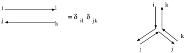
Figure 4: The Feynman rule of the $D=0$ dimensional matrix model. The left describes the propagator while the right describes the vertex.

We next investigate the contribution of the vertex. For the $\phi^{3}$ theory, the action including the interaction is

$$S_{int}=\frac{1}{2}TrM^{2}+\frac{\lambda}{3}TrM^{3}.$$ (2.32)

The way to take the sum with respect to the indices is described by the Feynman rule, as shown in Fig. 4. The vertex is ${\cal O}(\lambda)$. In this Feynman rule, the presence of the upper and lower matrix indices is represented by the double line, and this description inherits that of large $N$ QCD. This is a natural notation because $D=0$ dimensional QFT shares the structure of Feynman diagrams with large $N$ QCD.

We next explain the relationship between the string theory described by the ’random triangulation’ and the $D=0$ dimensional QFT. Consider the partition function of the above large $N$ matrix model with $\phi^{3}$ interaction

$$Z_{QFT}=\int d^{N^{2}}M\exp(-\frac{1}{2}TrM^{2}+\frac{g}{\sqrt{N}}TrM^{3}),$$ (2.33)

where $M$ is a hermitian matrix, and $\lambda$ is now replaced with $\lambda\to-\frac{g}{\sqrt{N}}$. Note that this integral is defined by the analytic continuation in the coupling constant $g$. We perform a Taylor expansion of the interaction term $\exp(\frac{g}{\sqrt{N}}TrM^{3})$. Then, this matrix integration is

$$Z_{QFT}=\sum_{n=0}^{\infty}\frac{1}{n!}(\frac{g}{\sqrt{N}})^{n}\int d^{N^{2}}M\exp(-\frac{1}{2}TrM^{2})(TrM^{3})^{n}.$$ (2.34)

The $n$-th power describes the system in which there are $n$ 3-point vertices in the world sheet. And the above Feynman rule shows that this system is described by gluing $n$ equilateral triangles described by fig. 3. Since each equilateral triangle possesses unit area,

$$A=(\textrm{area of the worldsheet})=(\textrm{number of triangles})=n.$$ (2.35)

We would like to identify this $D=0$ QFT with the partition function of the $D=0$ bosonic string theory. In this process, there are two identifications.

• We can immediately discern the identification $e^{-\beta}=g$

• The other is to identify $e^{\gamma}$ with the size of the matrices $N$. However, this is less trivial than the previous identification, and we need some explanation. To discern the identification $N=e^{\gamma}$, let us rescale this matrix model by $M\to M\sqrt{N}$. The action is then described by

  $$-\frac{1}{2}TrM^{2}+\frac{g}{\sqrt{N}}TrM^{3}\to N(-\frac{1}{2}TrM^{2}+gTrM^{3}).$$ (2.36)

  This rescale makes $N$ an overall factor, and the $N$ dependence of the Feynman rule becomes transparent.

  • Vertex: This is clearly ${\cal O}(N)$, because of the interaction term $gNTrM^{3}$.

  • Propagator: This is ${\cal O}(N^{-1})$, because of the formula $\int_{-\infty}^{\infty}x^{2}\exp(-\frac{ax^{2}}{2})dx=\frac{1}{a}\int_{-\infty}^{\infty}\exp(-\frac{ax^{2}}{2})dx$, with $a$ now being replaced by $N$.

  • Loop: This is ${\cal O}(N)$. To comprehend this statement, let us have a look at a simple case. Consider the diagram of $\langle M_{ij}M_{kl}\rangle$ in Fig. 4. There are $N$ ways to connect the indices for each of $\delta_{i}^{l}$ and $\delta_{j}^{k}$. This induces $\sum_{i,j,k,l=1}^{N}\delta_{i}^{l}\delta_{j}^{k}=N^{2}$. The total contribution is therefore ${\cal O}(N^{-1}N^{2})={\cal O}(N)$.

  These rules indicate that the total contribution of the power of $N$ is

  $${\cal O}(N^{V-E+F})={\cal O}(N^{\chi}),$$ (2.37)

  where $\chi$ is the Euler character of the diagram, which is with ease identified with the Euler character of the worldsheet of the string theory. Therefore, the identification $N=e^{\gamma}$ is justified.

This matrix model is formally identified with the string theory with on the discritized worldsheet by the identification of the quantities

$$g\leftrightarrow e^{-\beta},\hskip 8.53581ptN\leftrightarrow e^{\gamma}.$$ (2.38)

This is an evidence of the belief that string is described by a large $N$ reduced model. For $D\leq 1$, bosonic string theory is successfully quantized by Distler and Kawai[23] (as is in fact true of superstring theory). And as we will see later, the string susceptibility obtained by this matrix model matches the analysis of Distler and Kawai. Owing to the work of Distler and Kawai, the matrix model may make a transition from being a mere ’toy model’ to being a realistic nonperturbative description of string theory. An important remark is that this matrix model leaves only the leading order of $N^{\chi}=N^{2-2h}$ if we take a limit $N\to\infty$. This means that only the effect of planar Riemann surface(without genus) survives. We have seen a similar situation in large $N$ QCD, in which only the effect of planar Feynman diagram survives in large $N$ limit. Although we have hitherto emphasized only the random triangulation, this analysis extends to any ’polygonulation’ with ease. For example, in order to consider the Riemann surfaces approximated by many equilateral squares, we have only to consider the matrix model

$$Z_{QFT}=\int d^{N^{2}}M\exp(-\frac{1}{2}TrM^{2}+\frac{g}{N}TrM^{4})=\sum_{n=0}^{\infty}(\frac{g}{N})^{n}\int d^{N^{2}}M\exp(-\frac{1}{2}TrM^{2})(TrM^{4})^{n}.$$ (2.39)

The $n$-th power of this action describes the system in which there are $n$ 4-point vertices. This system is of grave importance in the analysis of pure gravity by Brezin and Kazakov in the subsequent section.

2.3 Orthogonal Polynomial Method

This section is devoted to introducing the method to analyze the above $D=0$ dimensional QFT in terms of large $N$ matrices. This method plays an essential role in solving this $D=0$ matrix model including the effect of higher genera, and thus makes the exact solution of this matrix model accessible. We start with the analysis of the matrix model

$$Z_{N}(g)=\int d^{N^{2}}M\exp(-V(M)).$$ (2.40)

Here, we focus on the pure gravity $V(M)=\frac{1}{2g}(TrM^{2}+\frac{1}{N}TrM^{4})$. This model is analyzed in terms of the eigenvalues $\{\lambda_{i}\}$ of the matrix $M$. The measure is known to be, whose proof we refer to Appendix. B.1,

$$d^{N^{2}}M=\prod_{i}d\lambda_{i}\prod_{i<j}(\lambda_{i}-\lambda_{j})^{2}dU_{ij}=\prod_{i=1}^{N}d\lambda_{i}(detX)^{2}dU_{ij},$$

$$\textrm{where }X=\left(\begin{array}[]{cccc}1&1&\cdots&1\\ \lambda_{1}&\lambda_{2}&\cdots&\lambda_{N}\\ \lambda^{2}_{1}&\lambda^{2}_{2}&\cdots&\lambda^{2}_{N}\\ \vdots&\vdots&\ddots&\vdots\\ \lambda^{N-1}_{1}&\lambda^{N-1}_{2}&\cdots&\lambda^{N-1}_{N}\end{array}\right).$$ (2.46)

Since the integrand depends only on the eigenvalues $\{\lambda_{i}\}$, the effect of the integral $dU_{ij}$ is trivial. In order to solve this matrix model, we introduce a series of orthogonal polynomials $\{P_{n}(\lambda)\}$ ($n=0,1,\cdots$) which enjoy the following two properties.

• $P_{n}(\lambda)$ is a polynomial of $n$-th degree, and the coefficient of the highest power of $\lambda$ is 1. There exists a series of coefficients $\{a_{n,j}\}$ such that $P_{n}(\lambda)=\lambda^{n}+\sum_{j=0}^{n-1}a_{n,j}\lambda^{j}$.

• These polynomials are orthogonal with respect to the integral

  $$\int_{-\infty}^{\infty}d\lambda\exp(-V(\lambda))P_{n}(\lambda)P_{m}(\lambda)=h_{n}\delta_{mn}.$$ (2.47)

  We call the quantity $h_{n}$ ’norm of $P_{n}(\lambda)$’.

Vandermonde’s determinant is rewritten as

$$\det\left(\begin{array}[]{cccc}1&1&\cdots&1\\ \lambda_{1}&\lambda_{2}&\cdots&\lambda_{N}\\ \lambda^{2}_{1}&\lambda^{2}_{2}&\cdots&\lambda^{2}_{N}\\ \vdots&\vdots&\ddots&\vdots\\ \lambda^{N-1}_{1}&\lambda^{N-1}_{2}&\cdots&\lambda^{N-1}_{N}\end{array}\right)=\det\left(\begin{array}[]{cccc}P_{0}(\lambda_{1})&P_{0}(\lambda_{2})&\cdots&P_{0}(\lambda_{N})\\ P_{1}(\lambda_{1})&P_{1}(\lambda_{2})&\cdots&P_{1}(\lambda_{N})\\ P_{2}(\lambda_{1})&P_{2}(\lambda_{2})&\cdots&P_{2}(\lambda_{N})\\ \vdots&\vdots&\ddots&\vdots\\ P_{N-1}(\lambda_{1})&P_{N-1}(\lambda_{2})&\cdots&P_{N-1}(\lambda_{N})\end{array}\right).$$ (2.58)

Going back to the very definition of the determinant,

$$\prod_{i,j=1}^{N}(\lambda_{i}-\lambda_{j})^{2}=\sum_{\sigma_{N}}(\prod_{i=1}^{N}P_{i}(\lambda_{\sigma_{N}(i)}))^{2},$$ (2.59)

where $\sigma_{N}(i)$ is the permutation, we readily obtain

$$Z_{N}(g)=N!\prod_{i=0}^{N-1}h_{i}=N!h_{0}^{N}\prod_{i=1}^{N-1}f_{k}^{N-k},$$ (2.60)

where $f_{k}=\frac{h_{k}}{h_{k-1}}$. We next seek the recursion formula of the orthogonal polynomials. The potential is here an even function $V(\lambda)=\frac{1}{2g}(\lambda^{2}+\frac{1}{N}\lambda^{4})$. We consider the expansion $\lambda P_{n}(\lambda)=\sum_{i=0}^{n+1}c_{n,i}P_{i}(\lambda)$ with $c_{n,n+1}=1$. Likewise, the other coefficients are given by $c_{n,i}=h_{i}^{-1}\int_{-\infty}^{\infty}d\lambda e^{-V(\lambda)}P_{n}(\lambda)P_{i}(\lambda)$. Utilizing these properties and the orthogonality of the polynomials, we readily obtain the following relationships.

• $c_{n,i}=0$ for $i=0,1,\cdots n-2$. This is trivial since $\lambda P_{i}(\lambda)$ can be expressed by the linear combination of $P_{0}(\lambda),P_{1}(\lambda),\cdots,P_{n-1}(\lambda)$.

• $c_{n,n-1}=h^{-1}_{n-1}\int_{-\infty}^{\infty}d\lambda e^{-V(\lambda)}P_{n}(\lambda)(P_{n}(\lambda)+\sum_{j=0}^{n-1}c_{n-1,j}P_{j}(\lambda))=h_{n}h^{-1}_{n-1}=f_{n}$.

• $c_{n,n}=0$ because the potential $V(\lambda)$ is an even function, whereas $\lambda(P_{n}(\lambda))^{2}$ is an odd function.

Therefore, we have succeeded in deriving the recursion formula

$$\lambda P_{n}(\lambda)=P_{n+1}(\lambda)+f_{n}P_{n-1}(\lambda).$$ (2.61)

Having obtained this relationship, we finally obtain the relationship amang the coefficients $\{f_{i}\}$. The integration ${\cal I}=\int_{-\infty}^{\infty}e^{-V(\lambda)}\frac{dP_{n}(\lambda)}{d\lambda}\lambda P_{n}(\lambda)$ can be evaluated in two ways.

• First, we consider the fact that

  $$\lambda\frac{dP_{n}(\lambda)}{d\lambda}=\lambda(n\lambda^{n-1}+\sum_{j=1}^{n-1}a_{n,j}j\lambda^{j-1})=n\lambda^{n}+\cdots.$$

  The above integral is readily given by ${\cal I}=nh_{n}$.

• The other way is to perform a partial integration. Here, we exploit an explicit form $V(\lambda)=\frac{1}{2g}(\lambda^{2}+\frac{1}{N}\lambda^{4})$. Then, the integral in question is

  $${\cal I}=\int_{-\infty}^{\infty}d\lambda e^{-V(\lambda)}\frac{dP_{n}(\lambda)}{d\lambda}f_{n}P_{n-1}=f_{n}\int_{-\infty}^{\infty}e^{-V(\lambda)}\frac{dV(\lambda)}{d\lambda}P_{n}(\lambda)P_{n-1}(\lambda).$$

  Exploiting the fact that $\frac{dV(\lambda)}{d\lambda}=\frac{\lambda}{g}+\frac{2\lambda^{3}}{gN}$, this integral is finally evaluated as

  $${\cal I}=\frac{1}{g}h_{n}f_{n}+\frac{2}{gN}f_{n}\int_{-\infty}^{\infty}d\lambda P_{n}(\lambda)\lambda^{2}(P_{n}(\lambda)+f_{n-1}P_{n-1}(\lambda))=\cdots=\frac{1}{g}f_{n}h_{n}+\frac{2}{gN}f_{n}h_{n}(f_{n-1}+f_{n}+f_{n+1}).$$

Combining these two results, we finally obtain a recursion formula

$$gn=f_{n}+\frac{2}{N}f_{n}(f_{n-1}+f_{n}+f_{n+1}).$$ (2.62)

2.3.1 Analysis of the Planar Limit

Our next job is to solve the recursion formula (2.62). For simplicity, we first consider the planar ($N\to\infty$) limit. We approximate the series $\{f_{k}\}$ by a continuous function

$$\frac{f_{n}}{N}\to f(\xi),\hskip 8.53581pt\frac{n\pm 1}{N}\to f(\xi\pm\epsilon),$$ (2.63)

where $\epsilon=\frac{1}{N}$ and $\xi=\frac{n}{N}$. Since we take a limit $N\to\infty$, we discard the effect of $\epsilon=\frac{1}{N}$. This gives

$$g\xi=f(\xi)+6f^{2}(\xi).$$ (2.64)

We define a new function $W(f)$ near its critical point $f\sim f_{c}$ as $W(f)=f+6f^{2}$. We consider the saddle point of the function $W(f)$ : $\frac{dW(f)}{df}=0$ at $f=f_{c}$. Defining $g_{c}$ as $g_{c}=W(f_{c})$, we obtain

$$g\xi=g_{c}+\frac{1}{2}W^{\prime\prime}(f_{c})(f(\xi)-f_{c})^{2}.$$ (2.65)

We compare this result with the quantized gravity. As we have explained before, the parameter named ’string susceptibility’ is defined as (2.18). String susceptibility $\gamma$ is expressed in the context of $D=0$ dimensional QFT as

$$f(\lambda)-f_{c}\sim(g_{c}-g\xi)^{-\gamma}.$$ (2.66)

The agreement of (2.66) with the very definition (2.18) can be verified by reflecting the correspondence between the matrix model and the string theory on the discritized worldsheet. Here, we have approximated the worldsheet by many equilateral square, because we are now considering the potential $V(\lambda)=\frac{1}{2g}(\lambda^{2}+\frac{1}{N}\lambda^{4})$. The area of the worldsheet is obviously

$$A=(\textrm{area of the worldsheet})=(\textrm{number of square})=n.$$ (2.67)

On the other hand, the partition function is given by (2.60). Taking the logarithm, we can approximate (2.60) by the continuous function

$$\frac{1}{N^{2}}Z=\frac{1}{N}\sum_{k=0}^{N-1}(1-\frac{k}{N})\log f_{k}\sim\int_{0}^{1}d\xi(1-\xi)\log f(\xi).$$ (2.68)

Performing the partial integration, we obtain a following remarkable relationship:

$$\frac{Z}{N^{2}} \sim \int_{0}^{1}d\xi(1-\xi)(f_{c}+(g_{c}-g\xi)^{-\gamma})\sim[(1-\xi)(g_{c}-g\xi)^{-\gamma+1}]_{0}^{1}+\int_{0}^{1}d\xi(g_{c}-g\xi)^{-\gamma+1}$$ (2.69)

$$\sim (g_{c}-g\xi)^{-\gamma+2}\sim\sum_{n=0}^{\infty}n^{\gamma-3}(\frac{g}{g_{c}})^{n}=\sum_{A=0}^{\infty}A^{\gamma-3}(\frac{g}{g_{c}})^{A}.$$

Thus, in order to seek a string susceptibility, we have only to consider the scaling of the function $f(\xi)$. In this case, the behavior of the critical point has been obtained in (2.65). Since $r(\xi)-r_{c}\sim(g\xi-g_{c})^{\frac{1}{2}}$. The string susceptibility is thus

$$\gamma=-\frac{1}{2}.$$ (2.70)

This is a result of planar ($N\times\infty$ and thus only the effect of $h=0$ survives) limit. Comparing this with the result in (2.19) [23], this corresponds to the result $D=0$ and $h=0$.

2.3.2 Analysis of the Nonplanar Behavior

We next consider the effect of higher genera to solve this matrix model exactly. The essential difference from the previous analysis is that we do not discard the term $\epsilon=\frac{1}{N}$. We use the function $W(r)=r+6r^{2}$, and we obtain

$$g\xi=g_{c}+\frac{1}{2}W^{\prime\prime}(r_{c})(r(\xi)-r_{c})^{2}+2r(\xi)(r(\xi+\epsilon)+r(\xi-\epsilon)-2r(\xi))=g_{c}+\frac{1}{2}W^{\prime\prime}(r_{c})(r(\xi)-r_{c})^{2}+2\epsilon^{2}\frac{d^{2}r}{d\xi^{2}}.$$ (2.71)

Now, we take the double scaling limit $N\to\infty$ and $g\to g_{c}$. $g-g_{c}$ possesses dimension $[\textrm{length}]^{2}$, and it is convenient to introduce a constant $a$ with dimension length. Then, let

$$g-g_{c}=\kappa^{-\frac{4}{5}}a^{2}.$$ (2.72)

And we assume an ansatz

$$\epsilon=\frac{1}{N}\stackrel{{\scriptstyle ansatz}}{{=}}a^{\frac{5}{2}}.$$

This is a maneuver to make the parameter $\kappa=(g-g_{c})^{-\frac{5}{4}}N^{-1}$ finite as we take the limit $N\to\infty$ and $g\to g_{c}$. In order to study this relationship, it is more convenient to change the variables as $g_{c}-g\xi=a^{2}z$. For this variables, we assume a following scaling ansatz

$$f(\xi)-f_{c}\stackrel{{\scriptstyle ansatz}}{{=}}au(z).$$ (2.73)

Then, we obtain a relationship $r(\xi+\epsilon)+r(\xi-\epsilon)-2r(\xi)\sim\epsilon^{2}\frac{d^{2}r}{d\xi^{2}}\sim a^{2}\frac{d^{2}u}{dz^{2}}$, utilizing $\epsilon\frac{d}{d\xi}=-ga^{\frac{1}{2}}\frac{d}{dz}$. Then, we obtain a nonlinear differential equation for the function $u(z)$ called Painleve equation:

$$z=u^{2}(z)+\frac{d^{2}u(z)}{dz^{2}}.$$ (2.74)

This equation provides us with a lot of information about the $D=0$ dimensional QFT. First, we can obtain an exact form of the function $f(\xi)$ from the solution of Painleve equation. Noting the relationship of the relationship of the partition function (2.60), this gives an exact form of the partition function of the theory! The orthogonal polynomial method plays a splendid role in solving the matrix model as $D=0$ dimensional QFT nonperturbatively. This is a great success of the matrix model in solving the string theory nonperturbatively, even though this discussion is limited to a very low spacetime dimension.

Furthermore, the analysis of the string susceptibility via orthogonal polynomial method agrees with the result of Distler and Kawai. In order to see this, let us consider the asymptotic solutions of Painleve equation. First, we consider the solution of (2.74) for $z\to\infty$. This corresponds to the planar behavior because we have taken a scaling $\epsilon=\frac{1}{N}=a^{\frac{5}{2}}$ and $g_{c}-g\xi=a^{2}z$, and hence $a$ should be $a\to 0$. The asymptotic solution is

$$u(z)=\sqrt{z},\hskip 5.69054pt(\textrm{as }z\to\infty).$$ (2.75)

This makes sense because because substituting this answer into the Painleve equation, $z=(\sqrt{z})^{2}-\frac{1}{4}z^{-\frac{3}{2}}\sim z$ (as $z\to\infty$). This means that the string susceptibility of the string without any genus is $\gamma=-\frac{1}{2}$, from the property (2.66). We next add a contribution of the subleading term. Let the solution of Painleve equation be

$$u(z)=\sqrt{z}+az^{b}.$$ (2.76)

Here, it is not the coefficient $a$ but the scaling $b$ that imports. Substituting this answer into Painleve equation, we obtain

$$z=z+2az^{\frac{1}{2}+b}+a^{2}z^{2b}-\frac{1}{4}z^{-\frac{3}{2}}+ab(b-1)z^{b-2}.$$ (2.77)

In order for the equality of the above equation to hold, the scaling parameter $b$ should satisfy

$$2b=b-2,\hskip 8.53581pt\frac{1}{2}+b=-\frac{3}{2}.$$ (2.78)

Both conditions are satisfied for $b=-2$. Them the solution including the subleading term is

$$u(z)=\sqrt{z}-\frac{1}{8}z^{-2}.$$ (2.79)

This indicates that the string susceptibility for $D=0$ and $h=1$ is $\gamma=2$. Repeating the same procedure, we obtain an asymptotic solution

$$u(z)=\sqrt{z}(1+\sum_{h=1}^{\infty}u_{h}z^{\frac{5h}{2}}),$$ (2.80)

where $\{u_{h}\}$ is a coefficient. This gives the string susceptibility for $D=0$ and all genera of the Riemann surface:

$$\gamma=2-\frac{5}{2}(1-h).$$ (2.81)

This agrees with the analysis of Distler and Kawai (2.19). This striking agreement of the string susceptibility further solidifies the confidence that the nonperturbative behavior of string theory is described by matrix model.

2.4 Summary

We would like to conclude this section by summarizing the argument in this section.

• Distler and Kawai succeeded in the quantization of both bosonic string and superstring for $D\leq 1$. And they computed a parameter ’string susceptibility’ for all genera of the worldsheet.

• The proposal that string should be described by matrix model was first given by F. David. He discritized the worldsheet of bosonic string theory into many polygons, and related the discritized theory with a matrix model describing 0 dimensional QFT.

• Brezin and Kazakov solved the 0 dimensional QFT via orthogonal polynomial method. Their answer describes the effects of higher genera of the worldsheet, and the string susceptibility for $D=0$ agrees with the results of Distler and Kawai.

These series of works are of historical importance in that they are the canons of the belief that matrix theory is the Ariadne’s thread to ’Theory of Everything’.

3 The brief review of IKKT Model

In the late 1990’s, several proposals for ’Theory of Everything’ have been given, reflecting the progress of the research of superstring theory. The belief that the nonperturbative behavior of string should be described by matrix theory has given three major proposals - BFSS model [4], IKKT model [5] and matrix string theory [6]. These proposals are the dimensional reduction of ${\cal N}=1$ SYM into 1, 0 and 2 dimensions respectively. Among them, the most successful proposal is IKKT model, and this section is devoted to the review of IKKT model.

3.1 Definition and Symmetry of IKKT model

Inspired by the discovery of BFSS conjecture, Ishibashi, Kawai, Kitazawa and Tsuchiya proposed a matrix theory described by the 0 dimensional reduction of ${\cal N}=1$ 10 dimensional SYM. This is IKKT model, whose action is

$$S=-\frac{1}{g^{2}}Tr(\frac{1}{4}\sum_{i,j=0}^{9}[A_{i},A_{j}][A^{i},A^{j}]+\frac{1}{2}\sum_{i,j=0}^{9}{\bar{\psi}}\Gamma^{i}[A_{i},\psi]).$$ (3.1)

• $A_{i}$ are $N\times N$ Hermitian matrices, and these are 10 dimensional vectors.

• $\psi$ are also $N\times N$ Hermitian matrices, and these are 10 dimensional Majorana-Weyl 16 spinors.

• Throughout this paper, the indices $i,j,\cdots$ refer to 10 dimensions, while $\mu,\nu,\cdots$ refer to 11 dimensions. And the trace $Tr$ is for $N\times N$ matrices in large $N$ reduced model.

• This matrix theory manifestly possesses $SO(9,1)$ Lorentz symmetry and $SU(N)$ gauge symmetry.

• This theory has no free parameter. The only parameter $g$ is absorbed into the fields by the rescaling $A_{i}\rightarrow g^{\frac{1}{2}}A_{i}$ and $\psi\rightarrow g^{\frac{3}{4}}\psi$.

This matrix theory has another name - IIB matrix theory -, because this theory is deeply related with type IIB superstring. There are several reasons to speculate that this model is a constructive definition of type IIB superstring, and one of these aspects is that this matrix model is the same as the matrix reguralization of the Schild action of type IIB superstring. First, let us introduce Green-Schwarz action of type IIB superstring, whose derivation we refer to [27]. We introduce a superspace for ${\cal N}=2$ superspace

$$Z^{M}=(X^{i},\theta^{1\alpha},\theta^{2\alpha}),$$ (3.2)

where $X^{i}$ are 10 dimensional vectors while two spinors $\theta^{1,2\alpha}$ are each 16 Majorana Weyl spinors for 10 dimensional spacetime (therefore, in total we have 32 spinors). For this superspace, the SUSY transformation is defined as

$$\delta_{S}X^{i}=i{\bar{\epsilon}^{1}}\Gamma^{i}\theta^{1}-i{\bar{\epsilon}^{2}}\Gamma^{i}\theta^{2},\hskip 5.69054pt\delta_{S}\theta^{1,2}=\epsilon^{1,2}.$$ (3.3)

The following quantities are SUSY invariant :

$$\Pi^{i}_{a}=\partial_{a}X^{i}-i{\bar{\theta}^{1}}\Gamma^{i}\partial_{a}\theta^{1}+i{\bar{\theta}^{2}}\Gamma^{i}\partial_{a}\theta^{2},\hskip 5.69054pt\Pi^{1,2\alpha}_{a}=\partial_{a}\theta^{1,2\alpha}.$$ (3.4)

The trouble is that the degree of freedom for fermions are much larger that that of bosons, the former being $16\times 2=32$, the latter being $11-2-1+8$. The maneuver to remedy this situation is to introduce Wess-Zumino term, whose explanation we owe to [27]. This maneuver is possible only for

$$D=\textrm{(dimensions of spacetime)}=3,4,6,10.$$ (3.5)

Then, the action should have another symmetry called $\kappa$ symmetry

$$\delta_{\kappa}X^{i}=i{\bar{\theta}^{1}}\Gamma^{i}\alpha^{1}-i{\bar{\theta}^{2}}\Gamma^{i}\alpha^{2},\hskip 5.69054pt\delta_{\kappa}\theta^{1,2}=\alpha^{1,2},$$ (3.6)

where

$$\alpha^{1}=(1+{\tilde{\Gamma}})\kappa_{1},\hskip 5.69054pt\alpha_{2}=(1-{\tilde{\Gamma}})\kappa^{2},\hskip 5.69054pt{\tilde{\Gamma}}=\frac{1}{2!\sqrt{-M}}\epsilon^{ab}\Pi^{i}_{a}\Pi^{j}_{b}\Gamma_{ij},\hskip 5.69054ptM=\det(\epsilon^{ab}\Pi^{i}_{a}\Pi^{j}_{b}),$$ (3.7)

$$\epsilon_{01}=+1\textrm{ (hence }\epsilon^{01}=-1\textrm{ ) }.$$ (3.8)

The action constructed to have these symmetry is the Green Schwarz form of the superstring possessing ${\cal N}=2$ symmetry:

$$S_{GS}=-T\int d^{2}\sigma[\sqrt{-M}+i\epsilon^{ab}\partial_{a}X^{i}({\bar{\theta}^{1}}\Gamma_{i}\partial_{b}\theta_{1}+{\bar{\theta}^{2}}\Gamma_{i}\partial_{b}\theta_{2})+\epsilon^{ab}({\bar{\theta}^{1}}\Gamma^{i}\partial_{a}\theta^{i})({\bar{\theta}^{2}}\Gamma_{i}\partial_{b}\theta^{2})].$$ (3.9)

Type IIB superstring is defined so that the chirality of two spinors are the same, and we set $\theta^{1}=\theta^{2}=\psi$. The action is rewritten as

$$S_{GS}=-T\int d^{2}\sigma(\sqrt{-m}+2i\epsilon^{ab}\partial_{a}X^{i}{\bar{\psi}}\Gamma_{i}\partial_{b}\psi),$$ (3.10)

where $m=\det(m_{ab})=\det(\partial_{a}X^{i}\partial_{b}X_{i})$. This action is ${\cal N}=2$ SUSY invariant provided we redefine the SUSY by mixing the original SUSY with $\kappa$ symmetry. The new SUSY is

$$\delta\theta^{1,2}=\delta_{S}\theta^{1,2}+\delta_{\kappa}\theta^{1,2}\hskip 5.69054pt\delta X^{i}=\delta_{S}X^{i}+\delta_{\kappa}X^{i},$$ (3.11)

where we choose $\kappa$ symmetry to be $\kappa_{1}=\frac{-\epsilon^{1}+\epsilon^{2}}{2},\kappa_{2}=\frac{\epsilon^{1}-\epsilon^{2}}{2}$. Then, setting the SUSY parameter as

$$\xi=\frac{\epsilon^{1}+\epsilon^{2}}{2},\hskip 5.69054pt\epsilon=\frac{\epsilon^{1}-\epsilon^{2}}{2}$$ (3.12)

we can express the ${\cal N}=2$ SUSY of the Green-Schwarz action as follows:

$$\delta^{(1)}_{\epsilon}\psi=\frac{1}{2}\sqrt{-m}m_{ij}\Gamma^{ij}\epsilon,\hskip 5.69054pt\delta^{(1)}_{\epsilon}X^{i}=4i{\bar{\epsilon}}\Gamma^{i}\psi,$$ (3.13)

$$\delta^{(2)}_{\xi}\psi=\xi,\hskip 5.69054pt\delta^{(2)}_{\xi}X^{i}=0,$$ (3.14)

where $m_{ij}=\epsilon^{ab}\partial_{a}X_{i}\partial_{b}X_{j}$.

Our next job is to rewrite this Green-Schwarz action into Schild form. Defining $g_{ab}$ as the metric of the worldsheet, and the Poisson bracket as $\{X,Y\}=\frac{1}{\sqrt{g}}\epsilon^{ab}\partial_{a}X\partial_{b}Y$, this action is rewritten as

$$S_{Sh}=\int d^{2}\sigma[\sqrt{g}\alpha(\frac{1}{4}\{X^{i},Y^{i}\}^{2}-\frac{i}{2}{\bar{\psi}}\Gamma^{i}\{X_{i},\psi\})+\beta\sqrt{g}].$$ (3.15)

This action is proven to be equivalent to the Green-Schwarz form of type IIB superstring. The ${\cal N}=2$ SUSY of this Schild action is

$$\delta^{(1)}_{\epsilon}\psi=-\frac{1}{2}m_{ij}\Gamma^{ij}\epsilon,\hskip 5.69054pt\delta^{(1)}X^{i}=i{\bar{\epsilon}}\Gamma^{i}\psi,$$ (3.16)

$$\delta^{(2)}_{\xi}\psi=\xi,\hskip 5.69054pt\delta^{(2)}_{\xi}X^{i}=0.$$ (3.17)

We perform a procedure called ’matrix regularization’, whose detailed explanation we again owe to [27]. This procedure is, simply speaking, the mapping from the Poisson bracket to the commutator of large $N$ matrices

$$-i[,]\leftrightarrow\{,\},\hskip 5.69054ptTr\leftrightarrow\int d^{2}\sigma\sqrt{g}.$$ (3.18)

The functions $X^{i}$ are now mapped into the $N\times N$ matrices $A^{i}$. and we obtain the action similar to the original proposal of IKKT model :

$$S=-\alpha(\frac{1}{4}Tr[A_{i},A_{j}][A^{i},A^{j}]+\frac{1}{2}Tr({\bar{\psi}}\Gamma^{i}[A_{i},\psi]))+\beta Tr{\bf 1}.$$ (3.19)

By dropping the term $\beta Tr{\bf 1}$ and setting $\alpha=\frac{1}{g^{2}}$, we reproduce the action of IKKT model (3.1) . In this sence, it can be fairly said that IKKT model is a concept related to type IIB superstring theory. And we speculate that the matrix regularization of type IIB superstring theory is the constructive definition of type IIB superstring.

Now, let us have a careful look at the SUSY of IKKT model. We have formulated the SUSY of Schild action of type IIB superstring. In IKKT model we consider that the matrix-regularized version of that SUSY is inherited. The ${\cal N}=2$ SUSY of IKKT model is then distinguished by

• homogeneous: $\delta^{(1)}_{\epsilon}\psi=\frac{i}{2}[A_{i},A_{j}]\Gamma^{ij}\epsilon,\hskip 5.69054pt\delta^{(1)}_{\epsilon}A_{i}=i{\bar{\epsilon}}\Gamma_{i}\psi$.
  The feature of the ’homogeneous SUSY’ is that this SUSY transformation depends on the matter fields $A_{i}$ and $\psi$. And this SUSY transformation vanishes if there is no matter field.

• inhomogeneous: $\delta^{(2)}_{\xi}\psi=\xi,\hskip 5.69054pt\delta^{(2)}_{\xi}A_{i}=0$.
  The feature of the ’inhomogeneous SUSY’ is that the translation survives without the matter fields.

The commutators of these SUSY’s give the following important results:

$$(1) [\delta^{(1)}_{\epsilon_{1}},\delta^{(1)}_{\epsilon_{2}}]A_{i}=0,\hskip 5.69054pt[\delta^{(1)}_{\epsilon_{1}},\delta^{(1)}_{\epsilon_{2}}]\psi=0,$$ (3.20)

$$(2) [\delta^{(2)}_{\xi_{1}},\delta^{(2)}_{\xi_{2}}]A_{i}=0,\hskip 5.69054pt[\delta^{(2)}_{\xi_{1}},\delta^{(2)}_{\xi_{2}}]=0,$$ (3.21)

$$(3) [\delta^{(1)}_{\epsilon},\delta^{(2)}_{\xi}]A_{i}=-i{\bar{\epsilon}}\Gamma_{i}\xi,\hskip 5.69054pt[\delta^{(1)}_{\epsilon},\delta^{(2)}_{\xi}]\psi=0.$$ (3.22)

(Proof) These properties can be verified by taking the difference of the two SUSY transformations.

1. This is the most complicated to compute. For the gauge field, we should consider the following transformation

   $$A_{i} \stackrel{{\scriptstyle\delta^{(1)}_{\epsilon_{2}}}}{{\rightarrow}} A_{i}+i\epsilon_{2}\Gamma_{i}\psi\stackrel{{\scriptstyle\delta^{(1)}_{\epsilon_{1}}}}{{\rightarrow}}A_{i}+i({\bar{\epsilon}_{1}}+{\bar{\epsilon}_{2}})\Gamma_{i}\psi-\frac{1}{2}{\bar{\epsilon}_{2}}\Gamma_{i}[A_{j},A_{k}]\Gamma^{jk}\epsilon_{1},$$ (3.23)

   $$A_{i} \stackrel{{\scriptstyle\delta^{(1)}_{\epsilon_{1}}}}{{\rightarrow}} A_{i}+i\epsilon_{1}\Gamma_{i}\psi\stackrel{{\scriptstyle\delta^{(1)}_{\epsilon_{2}}}}{{\rightarrow}}A_{i}+i({\bar{\epsilon}_{1}}+{\bar{\epsilon}_{2}})\Gamma_{i}\psi-\frac{1}{2}{\bar{\epsilon}_{1}}\Gamma_{i}[A_{j},A_{k}]\Gamma^{jk}\epsilon_{2}.$$ (3.24)

   Then, the commutator is

   $$[\delta^{(1)}_{\epsilon_{1}},\delta^{(1)}_{\epsilon_{2}}]A_{i}=-\frac{1}{2}{\bar{\epsilon}_{2}}\Gamma_{i}[A_{j},A_{k}]\Gamma^{jk}\epsilon_{1}+\frac{1}{2}{\bar{\epsilon}_{1}}\Gamma_{i}[A_{j},A_{k}]\Gamma^{jk}\epsilon_{2}.$$ (3.25)

   Utilizing the formula $\Gamma^{i}\Gamma^{jk}=\Gamma^{ijk}+\eta^{ij}\Gamma^{k}-\eta^{ik}\Gamma^{j}$(for a general property, see Appendix. A.2.3) and the properties of the fermions in Appendix. A.2.4 , we obtain

   $$[\delta^{(1)}_{\epsilon_{1}},\delta^{(1)}_{\epsilon_{2}}]A_{i}=2{\bar{\epsilon}_{1}}\Gamma^{k}\epsilon_{2}[A_{i},A_{k}].$$ (3.26)

   For the fermions, we have only to repeat the similar procedure:

   $$\psi \stackrel{{\scriptstyle\delta^{(1)}_{\epsilon_{2}}}}{{\to}} \psi+\frac{i}{2}[A_{i},A_{j}]\Gamma^{ij}\epsilon_{2}\stackrel{{\scriptstyle\delta^{(1)}_{\epsilon_{1}}}}{{\to}}\psi+\frac{i}{2}[A_{i},A_{j}]\Gamma^{ij}(\epsilon_{1}+\epsilon_{2})-[A_{i},{\bar{\epsilon}_{1}}\Gamma_{j}\psi]\Gamma^{ij}\epsilon_{2},$$ (3.27)

   $$\psi \stackrel{{\scriptstyle\delta^{(1)}_{\epsilon_{1}}}}{{\to}} \psi+\frac{i}{2}[A_{i},A_{j}]\Gamma^{ij}\epsilon_{1}\stackrel{{\scriptstyle\delta^{(1)}_{\epsilon_{2}}}}{{\to}}\psi+\frac{i}{2}[A_{i},A_{j}]\Gamma^{ij}(\epsilon_{1}+\epsilon_{2})-[A_{i},{\bar{\epsilon}_{2}}\Gamma_{j}\psi]\Gamma^{ij}\epsilon_{1}.$$ (3.28)

   Using the formula of Fierz transformation,

   $${\bar{\epsilon}_{1}}\Gamma_{j}\psi\Gamma^{ij}\epsilon_{2}={\bar{\epsilon}_{1}}\Gamma^{i}\epsilon_{2}\psi-\frac{7}{16}{\bar{\epsilon}_{1}}\Gamma^{k}\epsilon_{2}\Gamma_{k}\Gamma^{i}\psi-\frac{1}{16\times 5!}{\bar{\epsilon}_{1}}\Gamma^{k_{1}\cdots k_{5}}\epsilon_{2}\Gamma_{k_{1}\cdots k_{5}}\Gamma^{i}\psi+(\textrm{rank 3 term}),$$ (3.29)

   whose proof we present in Appendix A.2.6, we verify that the commutator of SUSY transformation is

   $$[\delta^{(1)}_{\epsilon_{1}},\delta^{(1)}_{\epsilon_{2}}]\psi=2[\psi,{\bar{\epsilon}_{1}}\Gamma^{i}\epsilon_{2}A_{i}].$$ (3.30)

   We explain some tips in arriving at the result (3.30).

   • The rank 3 term of (3.29) does not contribute because the fermions $\epsilon_{1},\epsilon_{2}$ are Majorana ones and hence the difference ${\bar{\epsilon}}_{1}\Gamma^{ijk}\epsilon_{2}-{\bar{\epsilon}}_{2}\Gamma^{ijk}\epsilon_{1}$ cancels due to the property presented in Appendix. A.2.4.

   • We discern that the second and third terms of the Fierz transformation (3.29) with the help of the equation of motion of IKKT model: id est, the SUSY transformation (3.20) hold true only on shell. We utilize the equation of motion

     $$\frac{dS}{d{\bar{\psi}}}=-\frac{1}{g^{2}}\Gamma^{i}[A_{i},\psi]=0.$$ (3.31)

     The second and third terms of (3.29) drops because this is proportional to the commutator $\Gamma^{i}[A_{i},\psi]$.

   Next, we note that the commutators of SUSY transformation (3.26) and (3.30) vanish up to the gauge transformation. The gauge transformation of IKKT model is to multiply the unitary matrix $\alpha\in U(N)$. The gauge transformation is expressed in the infinitesimal form as follows :

   $$A_{i},\psi\rightarrow A_{i}+i[A_{i},\alpha],\hskip 5.69054pt\psi+i[\psi,\alpha].$$ (3.32)

   The SUSY transformation (3.26) and (3.30) can be gauged away by the gauge parameter $\alpha=2{\bar{\epsilon}_{1}}\Gamma^{k}\epsilon_{2}A_{k}$. We now complete the proof of (3.20) up to the gauge transformation.

2. This is trivial because the SUSY $\delta^{(2)}_{\xi}$ involves only a constant.

3. This can be proven by taking the difference of these two transformations

   $$A_{i} \stackrel{{\scriptstyle\delta^{(2)}_{\xi}}}{{\to}} A_{i}\stackrel{{\scriptstyle\delta^{(1)}_{\epsilon}}}{{\to}}A_{i}+i{\bar{\epsilon}}\Gamma_{i}\psi\textrm{, whereas }A_{i}\stackrel{{\scriptstyle\delta^{(1)}_{\epsilon}}}{{\to}}A_{i}+i{\bar{\epsilon}}\Gamma_{i}\psi\stackrel{{\scriptstyle\delta^{(2)}_{\xi}}}{{\to}}A_{i}+i{\bar{\epsilon}}\Gamma_{i}(\psi+\xi),$$ (3.33)

   $$\psi \stackrel{{\scriptstyle\delta^{(2)}_{\xi}}}{{\to}} \psi+\xi\stackrel{{\scriptstyle\delta^{(1)}_{\epsilon}}}{{\to}}\psi+\xi+\frac{i}{2}\Gamma^{ij}[A_{i},A_{j}]\epsilon\textrm{, whereas }\psi\stackrel{{\scriptstyle\delta^{(1)}_{\epsilon}}}{{\to}}\psi+\frac{i}{2}\Gamma^{ij}[A_{i},A_{j}]\epsilon\stackrel{{\scriptstyle\delta^{(2)}_{\xi}}}{{\to}}\psi+\xi+\frac{i}{2}\Gamma^{ij}[A_{i},A_{j}]\epsilon.$$

This completes the proof of the commutation relation of the SUSY transformation.(Q.E.D.)

We take a linear combination of the SUSY transformation to diagonalize the SUSY transformation

$${\tilde{\delta}}^{(1)}=\delta^{(1)}+\delta^{(2)},\hskip 5.69054pt{\tilde{\delta}}^{(2)}=i(\delta^{(1)}-\delta^{(2)}).$$ (3.34)

We obtain a following ${\cal N}=2$ SUSY algebra

$$[{\tilde{\delta}}^{(1)}_{\epsilon},{\tilde{\delta}}^{(1)}_{\xi}]\psi=[{\tilde{\delta}}^{(1)}_{\epsilon},{\tilde{\delta}}^{(2)}_{\xi}]\psi=[{\tilde{\delta}}^{(2)}_{\epsilon},{\tilde{\delta}}^{(2)}_{\xi}]\psi=0,$$ (3.35)

$$[{\tilde{\delta}}^{(1)}_{\epsilon},{\tilde{\delta}}^{(1)}_{\xi}]A_{i}=[{\tilde{\delta}}^{(2)}_{\epsilon},{\tilde{\delta}}^{(2)}_{\xi}]A_{i}=-2i{\bar{\epsilon}}\Gamma_{i}\xi,\hskip 5.69054pt[{\tilde{\delta}}^{(1)}_{\epsilon},{\tilde{\delta}}^{(2)}_{\xi}]A_{i}=0.$$ (3.36)

We regard the SUSY ${\tilde{\delta}}^{(1)}$ and ${\tilde{\delta}}^{(2)}$ as a fundamental SUSY transformation. We now confirm that these fundamental SUSY transformations actually satisfy Haag-Lopuszanski-Sohnius extension of Coleman-Mandula theorem, in which the supercharges must satisfy

$$\{Q_{x},Q_{x}\}=P_{i},\hskip 8.53581pt[P_{i},Q_{x}]=0(\textrm{for }x=1,2),$$ (3.37)

where $P_{i}$ is an operator for the translation of the bosonic vector fields. We verify these statements (3.37) one by one, for the ${\cal N}=2$ SUSY transformation of IKKT model.

The former statement $\{Q_{x},Q_{x}\}=P_{i}$ is readily read off from the commutation relation (3.36). Let the supercharge $Q_{i}$ be the SUSY transformation $Q_{x}(\epsilon)={\tilde{\delta}}^{(x)}_{\epsilon}$. Then, the relation (3.36) means

$$[Q_{x}(\epsilon),Q_{x}(\xi)]=-2i{\bar{\epsilon}}\Gamma_{i}\xi=\textrm{ (translation of the bosonic field)}.$$ (3.38)

The anti-commutator in (3.37) is replaced with the commutator because the SUSY parameters are Grassmann odd quantities. This indicates that the commutator of the supercharge translates the bosonic vector fields by $a_{i}=-2i{\bar{\epsilon}}\Gamma_{i}\xi$, and thus we have confirmed the first statement of Haag-Lopuszanski-Sohnius theorem.

The latter statement $[P_{i},Q]=0$ is trivial. Since the fundamental SUSY transformations are expressed by the linear combinations of $\delta^{(1)}$ and $\delta^{(2)}$, we have only to compute the commutation relation between the translation $P_{i}$ and the SUSY transformations $\delta^{(1)},\delta^{(2)}$.

• First, we verify the commutation relation $[P_{i},\delta^{(1)}]=0$. This can be verified by taking the difference of the two paths for both matter fields and the fermionic fields.

  • $A_{i}\stackrel{{\scriptstyle P_{i}}}{{\to}}A_{i}+a_{i}\stackrel{{\scriptstyle\delta^{(1)}_{\epsilon}}}{{\to}}A_{i}+a_{i}+i{\bar{\epsilon}}\Gamma_{i}\psi$, whereas $A_{i}\stackrel{{\scriptstyle\delta^{(1)}_{\epsilon}}}{{\to}}A_{i}+i{\bar{\epsilon}}\Gamma_{i}\psi\stackrel{{\scriptstyle P_{i}}}{{\to}}A_{i}+a_{i}+i{\bar{\epsilon}}\Gamma_{i}\psi$.

  • $\psi\stackrel{{\scriptstyle P_{i}}}{{\to}}\psi\stackrel{{\scriptstyle\delta^{(1)}_{\epsilon}}}{{\to}}\psi$, whereas $\psi\stackrel{{\scriptstyle\delta^{(1)}_{\epsilon}}}{{\to}}\psi\stackrel{{\scriptstyle P_{i}}}{{\to}}\psi$.

  These indicate that the commutator $[P_{i},\delta^{(1)}]$ vanishes both for the bosons and the fermions.

• The second commutation relation $[P_{i},\delta^{(2)}]=0$ is also verified in the same fashion.

  • $A_{i}\stackrel{{\scriptstyle P_{i}}}{{\to}}A_{i}+a_{i}\stackrel{{\scriptstyle\delta^{(2)}_{\epsilon}}}{{\to}}A_{i}+a_{i}$, whereas $A_{i}\stackrel{{\scriptstyle\delta^{(2)}_{\epsilon}}}{{\to}}A_{i}+a_{i}\stackrel{{\scriptstyle P_{i}}}{{\to}}A_{i}+a_{i}$.

  • $\psi\stackrel{{\scriptstyle P_{i}}}{{\to}}\psi\stackrel{{\scriptstyle\delta^{(2)}_{\epsilon}}}{{\to}}\psi+\frac{1}{2}[A_{i},A_{j}]\Gamma^{ij}$, whereas $\psi\stackrel{{\scriptstyle\delta^{(2)}_{\epsilon}}}{{\to}}\psi+\frac{1}{2}[A_{i},A_{j}]\Gamma^{ij}\stackrel{{\scriptstyle P_{i}}}{{\to}}\psi+\frac{1}{2}[A_{i},A_{j}]\Gamma^{ij}$.

This, although trivial, completes the proof of the statement $[P_{i},Q]=0$.

The important point is that the SUSY transformation (3.36) triggers the interpretation of the spacetime as being a part of the degrees of freedom of the large $N$ matrices. IKKT model is a 0-dimensional quantum field theory, but the 10-dimensional spacetime emerges from the eigenvalues of the bosonic matrices $A_{\mu}$. In other words, suppose that

$$(x^{(1)}_{\mu},x^{(2)}_{\mu},\cdots,x^{(N)}_{\mu})$$ (3.39)

are the eigenvalues of $A_{\mu}$. Then, the distribution of the points $x^{(n)}=(x^{(n)}_{0},x^{(n)}_{1},\cdots,x^{(n)}_{9})$ constitutes the 10-dimensional spacetime. Under this interpretation, the transformation (3.36) generates the shift of this new spacetime by $-2i{\bar{\epsilon}}\Gamma_{i}\xi$ in the $i$-th direction.

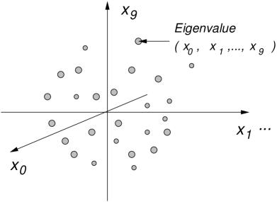
Figure 5: In IKKT model, the spacetimes are interpreted as the distribution of the eigenvalue of the bosonic matrices.

We have argued that IKKT model shares ${\cal N}=2$ SUSY with type IIB superstring. This is a crucial property for the theory to contain gravity. If this theory includes massless spectrum, this theory must contain spin 2 particles - graviton. And this is the very reason why we had to reduce the 10-dimensional, not the 4 or 6-dimensional, ${\cal N}=1$ SYM theory. Otherwise, this theory would not have the maximal 32 SUSY and thus could not be a theory of gravity.

It is known that IKKT model induces IIB supergravity by one-loop effects. Computing the effective Lagrangian around the 10 dimensional background, we see the effects of graviton exchange, however we omit the computation in this review.

3.2 Description of Many-Body system

We now have a look at the aspects of IKKT model as a many-body system. We have argued that the matters are described by the bosonic $N\times N$ matrices $A_{i}$. The amazing fact is that these large $N$ matrices can describe not only one-string effect but also multi-string effect. We concentrate on the simplest case - classical static D1-branes. We consider the classical equation of motion(EOM) of IKKT model, and hence we set the fermionic fields to be $\psi=0$. Since the action (3.1) does not contain a kinetic term for $A_{i}$, the EOM is

$$[A_{i},[A^{i},A^{j}]]=0.$$ (3.40)

Likewise, the EOM of Schild action of type IIB superstring is $\{X_{i},\{X^{i},X^{j}\}\}=0$. In terms of type IIB superstring, the solution of this EOM representing one D1-brane is

$$X^{0}=T\tau,\hskip 5.69054ptX^{1}=\frac{L}{2\pi}\sigma,\hskip 5.69054ptX^{2}=\cdots X^{9}=0,$$ (3.41)

where $T$ and $L$ are the compactification radii of $X^{0}$ and $X^{1}$ directions respectively. The parameters $\tau$ and $\sigma$ take values $0\leq\tau\leq 1$ and $0\leq\sigma\leq 2\pi$. Therefore, the Poisson bracket is computed to be

$$\{X^{0},X^{1}\}=\epsilon^{01}\partial_{0}X^{0}\partial_{1}X^{1}=\epsilon^{01}\frac{TL}{2\pi}=-\frac{TL}{2\pi}.$$ (3.42)

Translating this relation into the language of large $N$ matrices, we want matrices which satisfy

$$-i[A_{0},A_{1}]=\frac{TL}{2\pi N}\Leftrightarrow\{X_{0},X_{1}\}=(-1)\{X^{0},X^{1}\}=\frac{TL}{2\pi}.$$ (3.43)

Such a commutation relation is impossible if the size of the matrix $N$ is finite(this can be immediately seen by noting the cyclic property of trace $Tr$) , however taking the large $N$ limit we obtain a following solution

$$A_{0}=\frac{T}{\sqrt{2\pi N}}q,\hskip 5.69054ptA_{1}=\frac{L}{\sqrt{2\pi N}}p,$$ (3.44)

where $q$ and $p$ are infinite size matrices satisfying the commutation relation $[q,p]=+i$.

Likewise, we express multi-string states by the matrix theory. we consider the following two cases.

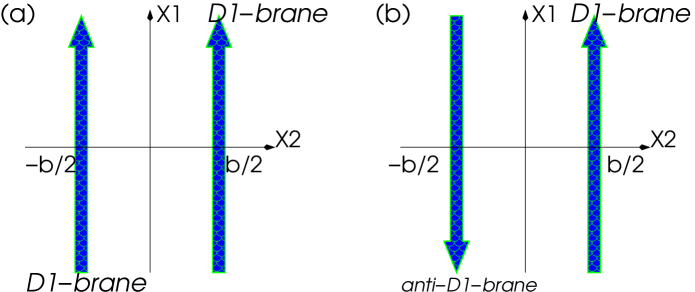
Figure 6: (a)$D1-D1$ brane system. (b)$D1-\overline{D1}$ brane system.

These systems are expressed in terms of the Schild type IIB superstring as

$$(a)\left\{\begin{array}[]{cc}X^{(1)0}=T\tau^{(1)}&X^{(2)0}=T\tau^{(2)}\\ X^{(1)1}=\frac{L}{2\pi}\sigma^{(1)}&X^{(2)1}=\frac{L}{2\pi}\sigma^{(2)}\\ X^{(1)2}=\frac{b}{2}&X^{(2)2}=-\frac{b}{2}\end{array}\right\},\hskip 14.22636pt(b)\left\{\begin{array}[]{cc}X^{(1)0}=T\tau^{(1)}&X^{(2)0}=T\tau^{(2)}\\ X^{(1)1}=\frac{L}{2\pi}\sigma^{(1)}&X^{(2)1}=-\frac{L}{2\pi}\sigma^{(2)}\\ X^{(1)2}=\frac{b}{2}&X^{(2)2}=-\frac{b}{2}\end{array}\right\}.$$ (3.51)

We likewise translate these systems into the language of matrix theory by means of matrix regularization. Using two independent pairs of matrices satisfying canonical commutation relation

$$[q,p]=+i,\hskip 5.69054pt[q^{\prime},p^{\prime}]=+i,$$ (3.52)

these two systems are described by block-diagonal matrices.

$$(a)A_{0}=\left(\begin{array}[]{cc}\frac{T}{2\pi n}q&0\\ 0&\frac{T}{2\pi n}q^{\prime}\end{array}\right)\equiv p_{0},\hskip 8.53581ptA_{1}=\left(\begin{array}[]{cc}\frac{T}{2\pi n}p&0\\ 0&\frac{T}{2\pi n}p^{\prime}\end{array}\right)\equiv p_{1},\hskip 8.53581ptA_{2}=\left(\begin{array}[]{cc}\frac{b}{2}&0\\ 0&-\frac{b}{2}\end{array}\right)\equiv p_{2},$$ (3.59)

$$(b)A_{0}=\left(\begin{array}[]{cc}\frac{T}{2\pi n}q&0\\ 0&\frac{T}{2\pi n}q^{\prime}\end{array}\right)\equiv p_{0},\hskip 8.53581ptA_{1}=\left(\begin{array}[]{cc}\frac{T}{2\pi n}p&0\\ 0&-\frac{T}{2\pi n}p^{\prime}\end{array}\right)\equiv p_{1},\hskip 8.53581ptA_{2}=\left(\begin{array}[]{cc}\frac{b}{2}&0\\ 0&-\frac{b}{2}\end{array}\right)\equiv p_{2},$$ (3.66)

where $n$ is a size of matrices $p,q,p^{\prime},q^{\prime}$ satisfying canonical commutation relation (3.52), hence $n$ should be large enough. We have now scratched a beautiful aspect of IKKT model - the matrices $A_{i}$ in this matrix theory can describe many-body system by taking block-diagonal matrices like the above-mentioned example. Extending this idea, many-body systems can be embedded in one large $N$ matrix. In this sense, IKKT model can be said to be a second quantization of superstring theory.

We have now seen the description of many-body system, in which multi-string states can be described by a block-diagonal matrix. This system does not include any interaction of each object. Then, how can we consider the interaction in this matrix model? The answer to this question lies in the off-diagonal part of the matrices.

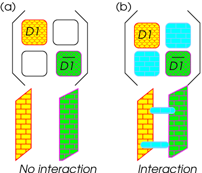
Figure 7: (a)The block diagonal matrices multi-string state including no interaction. (b)The off-diagonal part describes the interactions of multi-string states.

Here, we just sketch the idea of computing the interactions, and we leave the thorough explanation to [5] or [27]. As depicted by Fig. 7, the off-diagonal part plays an essential role in the interaction. We give an example only for the simplest case - $D1-D1$ brane and $D1-\overline{D1}$ brane system. We separate the matrix $A_{i}$ and $\psi$ into the background and the quantum fluctuation

$$A_{i}=p_{i}+a_{i},\hskip 5.69054pt\psi=\chi+\phi,$$ (3.67)

$p_{i}$ and $\chi$ being the background, and $a_{i}$ and $\phi$ being the quantum fluctuations. The action (3.1) is expanded up to the second order of the quantum fluctuations,

$$S_{2} = -Tr(\frac{1}{4}[p_{i},p_{j}][p^{i},p^{j}]+\frac{1}{2}{\bar{\chi}}[p_{i},\chi]-a_{j}([p_{i},[p^{i},p^{j}]]+\frac{1}{2}[{\bar{\chi}}\Gamma^{i},\chi])+{\bar{\psi}}\Gamma^{i}[p_{i},\phi]$$ (3.68)

$$+ \frac{1}{2}[p_{i},a_{j}][p^{i},a^{j}]-\frac{1}{2}[p_{i},a^{i}][p_{j},a^{j}]+[p_{i},p_{j}[a^{i},a^{j}]+\frac{1}{2}{\bar{\phi}}\Gamma^{i}[p_{i},\phi]+{\bar{\chi}}\Gamma^{i}[a_{i},\phi].$$

To fix the gauge invariance (3.32), we must add a gauge fixing term

$$S_{g.f.}=-Tr(\frac{1}{2}[p_{i},a^{i}][p_{j},a^{j}]+[p_{i},b][p^{i},c]).$$ (3.69)

The one-loop effective potential is given by the following path integral

$$W = -\log\int dad\phi dbdc\exp(-(S_{2}+S_{g.f.}))$$

$$= \frac{1}{2}Tr\log(P^{2}_{k}\delta_{ij}-2iF_{ij})-\frac{1}{4}Tr\log((P^{2}_{k}+\frac{i}{2}F_{ij}\Gamma^{ij})(\frac{1+\Gamma^{\sharp}}{2})-Tr\log(P^{2}_{k})+i\theta,$$

where $P_{i}X=[p_{i},X]$, $F_{ij}X=[f_{ij},X]=[[p_{i},p_{j}],X]$ and $\theta$ is an anomaly term which vanishes in these simplest cases. We skip the process to compute the interaction, and give only a result.

• For $D1-D1$ brane system, this effective potential is $W=0$, id est, there is no interaction between these two $D1$ branes. This is a natural result because the background $D1-D1$ system is supersymmetric, hence a stable system.

• For $D1-\overline{D1}$ brane system, the leading term of the effective potential is $W\propto b^{-6}$. This result agrees with the interaction of $D1-\overline{D1}$ brane in type IIB superstring theory.

This argument indicates that IKKT model succeeds in reproducing the interaction of $D1-\overline{D1}$ brane system. This result solidifies the belief that IKKT model is a constructive definition of type IIB superstring.

3.3 Noncommutative Yang-Mills(NCYM) in IKKT model

An important discovery in IKKT model is that this theory naturally induces noncommutative Yang-Mills theory by a simple mapping rule. The research of noncommutative Yang-Mills has recently become popular. We start with the idea of noncommutative space[12]. A noncommutative space refers to a space defined by

$$[x^{i},x^{j}]=i\theta^{ij},$$ (3.71)

where $\theta^{ij}$ is an antisymmetric quantity called ’noncommutative parameter’. What is the meaning of the relation $(\ref{AZM33NCspace})$ ? Note that the right-hand side is pure imaginary. This relation is reminiscent of the canonical commutation relation of the space coordinate and the momentum: $[q,p]=[q,-i\hbar\frac{\partial}{\partial q}]=+i\hbar$ (usually we adopt a God-given unit, and set $\hbar=1$). This canonical commutation relation causes the uncertainty relation between the space coordinate and its canonical momentum $(\Delta q)(\Delta p)\geq\frac{\hbar}{2}$ The same idea is inherited in the noncommutative geometry. The commutation relation (3.71) indicates the uncertainty relation between the space coordinates. This relation is a fundamental formula of ’the quantization of a space’. Utilizing the analogy of quantum mechanics, the physics of this space regards the coordinates as operators.

The noncommutativity of the space naturally emerges in superstring theory only by turning on B field [12]. This discovery is attractive because the understanding of such a difficult spacetime can be achieved with ease through superstring theory. According to the paper [12], for the string theory with NS B field, the commutation relation (3.71) is satisfied with the noncommutative parameter

$$\theta^{ij}=2\pi\alpha^{\prime}(\frac{1}{g+2\pi\alpha^{\prime}B})_{A}=-(2\pi\alpha^{\prime})^{2}(\frac{1}{g+2\pi\alpha^{\prime}B}B\frac{1}{g-2\pi\alpha^{\prime}B})^{ij},$$ (3.72)

which means that the coordinates possess the uncertainty

$$(\Delta x_{i})(\Delta x_{j})\geq\frac{1}{2}|\theta^{ij}|\sim{\cal O}(\alpha^{\prime})={\cal O}(\l_{s}^{2}).$$ (3.73)

The effect of the noncommutative space can be seen only if we consider the length scale as microscopic as the string length ${\cal O}(\l_{s})$ . This noncommutative theory is described by replacing the naive product of two operators with Moyal product

$$a(x)\star b(y)=\exp(\frac{i}{2}\theta^{ij}\frac{\partial^{2}}{\partial\xi^{i}\partial\eta^{\j}})a(x+\xi)b(y+\eta)|_{\xi=\eta=0}.$$ (3.74)

This technique is attractive in that it enables us to deal with the noncommutative field with the same ease as in the ordinary(commutative) fields.

Aoki, Ishibashi, Iso, Kawai, Kitazawa and Tada [11] pointed out that IKKT model naturally includes the noncommutative Yang-Mills(NCYM) theory. This result is not surprising, because a matrix is by nature a noncommutative object. The classical EOM of IKKT model (3.1) is expressed by (3.40). We pick up a set of classical solutions which satisfies

$$[{\hat{p}_{i}},{\hat{p}_{j}}]=iB_{ij},$$ (3.75)

where $B_{ij}$ are c-numbers (therefore, it is trivial that this solution (3.75) satisfies (3.40)). Of course this commutation relation cannot be satisfied for the finite size of the matrices $N$, however it is possible to approximate this solution by matrices whose size $N$ is large enough. Let ${\tilde{d}}$ be the rank of the matrices $B_{ij}$. And we separate the matrices $A_{i}$ between the classical solution and its quantum fluctuation $A_{i}={\hat{p}_{i}}+{\hat{a}_{i}}$. We perform Fourier transformation on the quantum fluctuation

$${\hat{a}}_{i}=\sum_{k}{\tilde{a}}_{i}(k)\exp(iC^{ij}k_{i}{\hat{p}}_{j}),\hskip 5.69054pt{\hat{\psi}}=\sum_{k}{\tilde{\psi}}(k)\exp(iC^{ij}k_{i}{\hat{p}}_{j}),$$ (3.76)

where $C^{ij}$ is an inverse matrix of $B_{ij}$ (id est, $C^{ij}B_{jk}=\delta^{i}_{k}$). Because the matrices are hermitian, we require that ${\tilde{a}}^{\star}(k)={\tilde{a}}(-k)$ and ${\tilde{\psi}}^{\star}(k)={\tilde{\psi}}(-k)$. Note that there is no classical part of the fermion because $\psi=0$ in the classical solution. In order to gain insight into the correspondence between the matrix model and NCYM, we put together several properties of this Fourier transformation.

Let us first consider the product of the Fourier transformation of two matrices ${\hat{a}}_{i}=\sum_{k}{\tilde{a}}_{i}(k)\exp(iC^{lm}k_{l}{\hat{p}}_{m})$ and ${\hat{b}}_{j}=\sum_{k}{\tilde{b}}_{j}(k)\exp(iC^{lm}k_{l}{\hat{p}}_{m})$. Utilizing Baker-Campbell-Hausdorff(BCH) formula $e^{A}e^{B}=\exp(A+B+\frac{1}{2}[A,B]\cdots)$, we obtain

$${\hat{a}_{i}}{\hat{b}_{j}} = \sum_{k,l}{\tilde{a}}_{i}(k){\tilde{b}}_{j}(l)\exp(iC^{rs}k_{r}{\hat{p}}_{s})\exp(iC^{tu}l_{t}{\hat{p}}_{u})=\sum_{k,l}{\tilde{a}}_{i}(k){\tilde{b}}_{j}(l)\exp(iC^{rs}(k_{r}+l_{r}){\hat{p}}_{s}+\frac{i^{2}}{2}C^{rs}C^{tu}k_{r}l_{t}iB_{su})$$ (3.77)

$$= \sum_{k,l}{\tilde{a}}_{i}(k){\tilde{b}}_{j}(l)\exp(iC^{rs}(k_{r}+l_{r}){\hat{p}}_{s}+\frac{-1}{2}C^{rs}C^{tu}k_{r}l_{t}i(-B_{us}))$$

$$= \sum_{k,l}{\tilde{a}}_{i}(k){\tilde{b}}_{j}(l)\exp(iC^{rs}(k_{r}+l_{r}){\hat{p}}_{s}+\frac{i}{2}C^{rs}k_{r}l_{s}).$$

Next we consider the trace of this matrix theory in the simplest case : 2 dimensional system. In this system, the noncommutative parameter is $B_{ij}\left(\begin{array}[]{cc}0&-B\\ B&0\end{array}\right)$ (hence $C^{ij}=\left(\begin{array}[]{cc}0&B^{-1}\\ -B^{-1}&0\end{array}\right)$). And let the classical solution be the canonical pairs ${\hat{p}_{0}}={\hat{q}}$ and ${\hat{p}_{1}}={\hat{p}}$ such that $[{\hat{q}},{\hat{p}}]=+i$. Then we obtain, utilizing BCH formula,

$$Tr\exp(iC^{ij}k_{i}{\hat{p}}_{j}) = Tr\exp(iB^{-1}(k_{0}{\hat{p}}-k_{1}{\hat{q}}))=\int dq\langle q|\exp(ik_{0}{\hat{p}}B^{-1})\exp(-ik_{1}{\hat{q}}B^{-1})\exp(ik_{0}k_{1}B^{-1})|q\rangle$$ (3.78)

$$= 2\pi B\delta(k_{0})\delta(k_{1})=(2\pi)^{2}\frac{1}{2\pi}\sqrt{\det B}\delta(k_{0})\delta(k_{1}).$$

Lastly let us see the effect of the adjoint operator $P_{i}{\hat{o}}\stackrel{{\scriptstyle def}}{{=}}[{\hat{p}_{i}},{\hat{o}}]$. This acts on ${\hat{a}_{i}}$ as

$$P_{i}{\hat{a}_{j}}=[{\hat{p}_{i}},{\hat{a}_{j}}]=\sum_{k}{\tilde{a}}_{j}(k)[{\hat{p}_{i}},\exp(iC^{lm}k_{l}{\hat{p}}_{m})]=\sum_{k}k_{i}{\tilde{a}}_{j}\exp(iC^{lm}k_{l}{\hat{p}}_{m}).$$ (3.79)

Having these results (3.77), (3.78) and (3.79) in mind, we consider the mapping rule which transforms IKKT into NCYM. The key to this crucial relationship is very simple:

$${\hat{a}}_{i}\textrm{(IKKT)}\Rightarrow a_{i}(x)=\sum_{k}{\tilde{a}}_{i}(k)\exp(ik_{j}x^{j})\textrm{(NCYM)}.$$ (3.80)

• This is a mapping from a $N\times N$ matrix to a c-number function. As we shall see later, this is a mapping into $U(1)$ NCYM theory.

• The relationship (3.77) indicates that the product of matrices is mapped into Moyal product in the language of NCYM,

  $${\hat{a}_{i}}{\hat{b}_{j}}\Rightarrow a_{i}(x)\star b_{j}(x)\equiv\exp(\frac{iC^{lm}}{2}\frac{\partial^{2}}{\partial\xi^{l}\partial\eta^{m}})a_{i}(x+\xi)b_{j}(x+\eta)|_{\xi=\eta=0}.$$ (3.81)

  This relationship has a profound significance, in that the residual phase factor in BCH formula induces the noncommutativity of the space in the mapped world. This is the very reason why we regard the mapped world as the noncommutative spacetime.

• The relationship (3.78) indicates that the trace of $N\times N$ matrices is translated into the integration over the spacetime,

  $$Tr({\hat{a}_{i}})\Rightarrow\sqrt{\det B}(\frac{1}{2\pi})^{\frac{{\tilde{d}}}{2}}\int d^{\tilde{d}}xa(x),$$ (3.82)

  where ${\tilde{d}}$ is the rank of the matrix $B_{ij}$, which equals to the spacetime dimensions of the mapped world.

• The relationship (3.79) indicates that the adjoint operator $P_{i}$ is interpreted as a differential operator in the world of ${\tilde{d}}$ dimensional NCYM theory:

  $$P_{i}{\hat{a}}_{j}(=[p_{i},{\hat{a}_{j}}])\Rightarrow-i\partial_{i}.$$ (3.83)

  Therefore, the commutator with the matrices of IKKT model $A_{i}$ is translated into the covariant derivative:

  $$[A_{i},{\hat{o}}]=[{\hat{p}}_{i}+{\hat{a}}_{i},{\hat{o}}]\Rightarrow D_{i}o(x)\stackrel{{\scriptstyle def}}{{=}}-i\partial_{i}o(x)+a_{i}(x)\star o(x)-o(x){\star}a_{i}(x).$$ (3.84)

  Especially, the commutator with two covariant derivative is a field strength

  $$[A_{i},A_{j}]\Rightarrow-i(\partial_{i}a_{j}(x)-\partial_{j}a_{i}(x))+[a_{i}(x),a_{j}(x)]_{\star}\equiv F_{ij}.$$ (3.85)

• This mapping rule induces the coordinate from the momentum in IKKT model. Having a careful look at the mapping rule (3.80), the coordinate in NCYM is produced from the IKKT model:

  $$C^{ij}{\hat{p}}_{j}\Rightarrow x^{i}.$$ (3.86)

  This correspondence possesses a profound meaning. We have before argued that the noncommutativity of the space (3.71) is a quantization of the space, just as the commutator of the coordinate and the momentum is nonzero in ordinary quantum mechanics. That the coordinate is naturally induced from the momentum strongly solidifies the correspondence between the ordinary quantum mechanics and the noncommutative geometry as the quantization of spacetime.

These are the profound features of the simple mapping rule (3.80). Note that the long wavelength excitations $|k|\ll\lambda$ ($\lambda$ refers to the spacing of the quanta) are commutative, again utilizing BCH formula,

$$[{\hat{a}}_{i},{\hat{a}}_{j}] = \sum_{k,l}{\tilde{a}}_{i}(k){\tilde{b}}_{j}(l)[\exp(iC^{rs}k_{r},{\hat{p}}_{s}),\exp(iC^{tu}l_{t}{\hat{p}}_{u})]$$ (3.87)

$$= \sum_{k,l}{\tilde{a}}_{i}(k){\tilde{a}}_{j}(l)\exp(iC^{rs}(k_{r}+l_{r}){\hat{p}}_{s})(\exp(\frac{i^{2}}{2}C^{rs}C^{tu}k_{r}l_{s}iB_{su})-\exp(\frac{i^{2}}{2}C^{rs}C^{tu}k_{r}l_{s}iB_{us}))$$

$$\stackrel{{\scriptstyle B_{su}=-B_{us}}}{{=}} 2i\sum_{k,l}{\tilde{a}}_{i}(k){\tilde{a}}_{j}(l)\exp(iC^{rs}(k_{r}+l_{r}){\hat{p}}_{s})\sin(\frac{1}{2}C^{rs}k_{r}l_{s}).$$

The low energy limit $|k|\ll\lambda$ is regarded as the semiclassical limit of the space $x^{i}=C^{ij}{\hat{p}}_{j}$. Then, IKKT model is (when the rank of $B_{ij}$ is ${\tilde{d}}$), mapped into ${\tilde{d}}$ dimensional NCYM theory

$$-\frac{1}{g^{2}}Tr(\frac{1}{4}[A_{i},A_{j}][A^{i},A^{j}]+\frac{1}{2}{\bar{\psi}}\Gamma^{i}[A_{i},\psi])$$ (3.88)

$$\Rightarrow \frac{{\tilde{d}}nB^{2}}{4g^{2}}-\sqrt{\det B}(\frac{1}{2\pi})^{\frac{\tilde{d}}{2}}\int d^{\tilde{d}}x\frac{1}{g^{2}}(\frac{1}{4}F_{ab}F^{ab}+\frac{1}{2}[D_{a},\alpha_{\rho}][D^{a},\alpha^{\rho}]+\frac{1}{4}[\alpha_{\rho},\alpha_{\chi}][\alpha^{\rho},\alpha^{\chi}]$$

$$+ \frac{1}{2}({\bar{\psi}}\Gamma^{a}[D_{a},\psi]+{\bar{\psi}}\Gamma^{\rho}[\alpha_{\rho},\psi]))_{\star}.$$

• The resulting NCYM theory possesses a gauge group $U(1)$ because the matrix in IKKT model is mapped into functions. The Yang-Mills coupling is now $g_{YM}=g^{2}(\frac{2\pi}{B})^{\frac{\tilde{d}}{2}}$.

• The indices $a,b,\cdots$ run over ${\tilde{d}}$ dimensional spacetime in the mapped NCYM theory. As we have before remarked, the commutator of the covariant derivative is a field strength $F_{ab}\stackrel{{\scriptstyle def}}{{=}}[D_{a},D_{b}]_{\star}$.

• The indices $\rho,\chi,\cdots$ here runs the transverse dimensions. In this residual dimension, there is no differentiation with respect to the field, and hence $D_{\rho}=\alpha_{\rho}$, where we have replaced $a_{\rho}\rightarrow\alpha_{\rho}$.

In order to extend this result to NCYM theory with gauge group $U(m)$, we have only to map the matrices in IKKT model into $m\times m$ matrices. The argument is totally parallel to the $U(1)$ case, and we replace element of ${\hat{p}}_{i}$ with

$${\hat{p}}_{i}\rightarrow{\hat{p}}_{i}\otimes{\bf 1}_{m}.$$ (3.89)

The Fourier decomposition is similar to the $U(1)$ case:

$${\hat{a}}_{i}=\sum_{k}{{\tilde{a}}_{i}(k)}_{m\times m}\exp(iC^{ij}k_{i}{\hat{p}}_{j}),\hskip 5.69054pt{\hat{\psi}}=\sum_{k}{{\tilde{\psi}}(k)}_{m\times m}\exp(iC^{ij}k_{i}{\hat{p}}_{j}).$$ (3.90)

The difference is that ${\tilde{a}}_{i}(k)$ and ${\tilde{\psi}}(k)$ are now $m\times m$ matrices (from now on we omit _m×m). Therefore, the mapping rule is

$${\hat{a}}_{i}(\in M_{N\times N})\Rightarrow a_{i}(x)=\sum_{k}{\tilde{a}}_{i}(k)\exp(ik_{j}x^{j})(\in M_{m\times m}),$$ (3.91)

where $M_{N\times N}$ is a set of $N\times N$ matrices. The resulting NCYM theory is similar to (3.88), except that the mapped theory is with respect to $U(m)$ matrices, and hence the theory is non-abelian.

3.4 Summary

We have seen many beautiful properties of IKKT model.

• IKKT model is defined as the 0 dimensional reduction of ${\cal N}=1$ 10 dimensional SYM theory. And this theory is the same as the matrix regularization of the Schild form of type IIB superstring theory.

• IKKT model possesses no free parameter. The coupling constant can be absorbed into the field by the rescaling $A_{i}\rightarrow g^{\frac{1}{2}}A_{i}$ and $\psi\rightarrow g^{\frac{3}{4}}\psi$.

• IKKT model possesses ${\cal N}=2$ supersymmetry, which is one of the essential properties of type IIB superstring. This indicates that the theory should include spin 2 gravitons if this theory has massless particles.

• IKKT model has an ability to describe many-body system only by one set of the matrices $A_{i}$. We have scratched the simplest case - how to describe $D1$-brane or anti-$D1$-brane. The computation of the interaction of $D1-\overline{D1}$ brane based on this matrix theory beautifully reproduces the result of type IIB superstring theory.

• IKKT model naturally induces NCYM theory by a simple mapping from a momentum in IKKT to a coordinate NCYM, $x^{i}=C^{ij}{\hat{p}}_{j}$. This strongly serves to solidify the correspondence between quantum mechanics and the noncommutative geometry as the quantization of spacetime.

There are other exciting properties of IKKT model. We list up some of the properties, but we omit the explanation.

• Schwinger-Dyson equation of the action of IKKT model induces the light-cone string field theory of type IIB superstring theory.

• Utilizing the analogy of branched polymer, it is possible to gain insight into how to induce our 4 dimensional world. We consider the branched polymer as the simplified model of the effective action of the spacetime points. The Hausdorff dimension of the branched polymer point is known to be 4.

IKKT is a successful proposal for the constructive definition of superstring, and possesses many exciting properties, which solidifies the confidence that it is a constructive definition.

4 $osp(1|32,R)$ Cubic Matrix Model

We have reviewed the successful aspects of the attempt to describe superstring theory in terms of matrix theory, and IKKT model indicates many promising aspects to be regarded as ’Theory of Everything’. Yet it is worth while to pursue a model exceeding IKKT model. L. Smolin presented a new approach to describe M-theory based on a simple matrix model [13]. This theory describes a dynamics of a matrix which is built from the super Lie algebra $osp(1|32,R)$. The action of this model, suggested by L. Smolin is described by a simple cubic action, as we discuss later in detail. There are several reasons we regard this model as attractive.

The action suggested by L. Smolin is extremely simple. The dream of elementary particle physics is to pursue a ’Theory of Everything’ from which all the phenomena of the whole universe are derived. Once Einstein found that the mechanics including the effect of gravity is described by general relativity, and the Lagrangian of this theory $I=\int d^{d}x\sqrt{g}R$ is extremely simple. We have a belief that the ’mother of the whole physical theory’ should be described by a simple action. The proposal for the constructive definition of superstring theory was suggested by Ishibashi, Kawai, Kitazawa and Tsuchiya. This is a dimensional reduction of ${\cal N}=1$ SYM theory, and this proposal is described by a simple and beautiful action, even though this proposal was once criticized as not as beautiful as general relativity. That the theory exceeding IKKT model may be described by a simple action is an attractive proposal, worth pursuing its validity and structure.

$osp(1|32,R)$ has been known as the unique maximal simple super Lie algebra with 32 fermionic generators [15]. This theory indicates a possibility that this may naturally include the existing matrix models, IKKT model or BFSS model. $osp(1|32,R)$ super Lie algebra, expressed in terms of 10 dimensional representation, includes two chiral spinors of both opposite chirality(IIA) and the same chirality(IIB). In this sense, we find $osp(1|32,R)$ super Lie algebra a natural framework for describing ’Theory of Everything’, and we are inclined to speculate that L. Smolin’s proposal is the clue to the ultimate theory.

That the theory is expressed by a cubic action possesses a profound significance in two senses. One aspect is that the fundamental interaction of superstring theory is a three-point interaction, because four (or more) point interaction is identified with three-point interaction by conformal invariance of the Feynman graphs. Thus it is a quite natural idea that the ’Theory of Everything’ which describes superstring theory comprehensively is a cubic matrix theory.

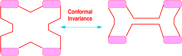
Figure 8: The fundamental interaction of string theory is a cubic one.

The other respect is that cubic action of string theory is identified with a Chern-Simons theory if a due compactification is performed. Chern-Simons theory is known to be exactly solvable by means of Jones Polynomial in knot theory [24]. If we find a correspondence between the cubic matrix model and Witten’s technique of solving Chern-Simons theory, we may be able to solve exactly the behavior of superstring in nonperturbative region, just as Brezin and Kazakov succeeded in solving exactly the bosonic string in 0 spacetime dimension via orthogonal polynomial method.

This theory deals with 11 dimensional spacetime, in terms of the 11 dimensional representation of $osp(1|32,R)$ super Lie algebra. And this theory may be able to describe superstring theory in such curved 10 dimensional spacetimes as $S_{1}\times R_{9}$ or $AdS_{5}\times S^{5}$, as well as a flat 10 dimensional spacetime.

This new proposal for describing superstring theory in terms of a supermatrix theory includes many interesting possibility, and the investigation of this cubic supermatrix theory is a fascinating issue.

4.1 Definition of $osp(1|32,R)$ super Lie Algebra

Before entering the investigation of the superstring action, we settle the definition of a super Lie algebra. A super Lie algebra is an algebra of supermatrix in which both bosonic matrices and the fermionic matrices are embedded in one matrix. Supermatrices possess many properties different from (ordinary) matrices, and these properties and the notations are summarized in detail in Appendix. A.3.

Let us start with the definition of $osp(1|32,R)$ super Lie algebra.

$$\clubsuit \textrm{ If }M\in osp(1|32,R),\textrm{ then }{{}^{T}M}G+GM=0\textrm{ for }G=\left(\begin{array}[]{cc}\Gamma^{0}&0\\ 0&i\end{array}\right).$$

$$\clubsuit M\textrm{ is traceless with respect to 33 }\times\textrm{ 33 supermatrix.}$$

$$\clubsuit M\textrm{ is a real supermatrix in that }M^{\ast}=M.$$

We confirm that, for the first condition, $osp(1|32,R)$ forms a closed super Lie algebra. Suppose matrices $M_{1}$ and $M_{2}$ satisfy the condition

$${{}^{T}M_{1}}G+GM_{1}=0,\hskip 11.38109pt{{}^{T}M_{2}}G+GM_{2}=0.$$ (4.4)

If $osp(1|32,R)$ is to be a closed super Lie algebra, we call for a following condition

$${{}^{T}([M_{1},M_{2}])}G+G[M_{1},M_{2}]=0.$$ (4.5)

Multiplying $G^{-1}$ on both (4.4) and (4.5) from the left, they are respectively rewritten as

$$G^{-1}{{}^{T}M_{k}}G+M_{k}=0,$$ (4.6)

$$G^{-1}{{}^{T}([M_{1},M_{2}])}G+[M_{1},M_{2}]=0,$$ (4.7)

where $k=1,2$. The proof that $osp(1|32,R)$ is a closed super Lie algebra is equivalent to deriving (4.7) utilizing (4.6):

$$\textrm{(\ref{AZMspade2+})}=[G^{-1}{{}^{T}M_{2}}G,G^{-1}{{}^{T}M_{1}}G]+[M_{1},M_{2}]\stackrel{{\scriptstyle(\ref{AZMspade1+})}}{{=}}[-M_{2},-M_{1}]+[M_{1},M_{2}]=0.$$ (4.8)

This statement, per se, can be satisfied whatever the matrix $G$ may be so long as $G$ has an inverse matrix.

Here comes one question:

Why do we define a metric $G$ as $G=\left(\begin{array}[]{cc}\Gamma^{0}&0\\ 0&i\end{array}\right)$ ?

This stems from the requirement that $M$ is a real matrix in that $M^{\ast}=({{}^{T}M})^{\dagger}=M$. Let us consider the consistency between this reality condition and the very definition of $osp(1|32,R)$ super Lie algebra. Take a hermitian conjugate of the definition ${{}^{T}M}G+GM=0$. This gives

$$G^{\dagger}({{}^{T}M})^{\dagger}+M^{\dagger}G^{\dagger}=0.$$ (4.9)

Utilizing the properties introduced in the Appendix. A.3.3, and the reality condition, this is rewritten as

$$0=G^{\dagger}({{}^{T}M})^{\dagger}+M^{\dagger}G^{\dagger}\stackrel{{\scriptstyle M^{\ast}=({{}^{T}M})^{\dagger}}}{{=}}G^{\dagger}M^{\ast}+M^{\dagger}G^{\dagger}\stackrel{{\scriptstyle M^{\dagger}={{}^{T}(M^{\ast})}}}{{=}}G^{\dagger}M^{\ast}+{{}^{T}(M^{\ast})}G^{\dagger}\stackrel{{\scriptstyle M=M^{\ast}}}{{=}}G^{\dagger}M+{{}^{T}M}G^{\dagger}.$$ (4.10)

In order for the relationship (4.10) to be consistent with the very definition of $osp(1|32,R)$, we must call for a condition

$$G^{\dagger}=G.$$ (4.11)

And the starting point of $osp(1|32,R)$ is well-defined if we take a metric as $G=\left(\begin{array}[]{cc}\Gamma^{0}&0\\ 0&i\end{array}\right)$.

The next issue is to investigate the explicit form of this super Lie algebra. This is expressed by

$$\textrm{ If }M\in osp(1|32),\textrm{ then }M=\left(\begin{array}[]{cc}m&\psi\\ i{\bar{\psi}}&0\end{array}\right).$$ (4.14)

• $m$ contains only the terms of rank 1,2,5. In other words, $m$ is expressed as

  $$m=u_{\mu_{1}}\Gamma^{\mu_{1}}+\frac{1}{2!}u_{\mu_{1}\mu_{2}}\Gamma^{\mu_{1}\mu_{2}}+\frac{1}{5!}u_{\mu_{1}\cdots\mu_{5}}\Gamma^{\mu_{1}\cdots\mu_{5}}.$$ (4.15)

• Here ${\bar{\psi}}$ denotes $\psi^{\dagger}\Gamma^{0}$. However, this is equivalent to ${{}^{T}\psi}\Gamma^{0}$, because we are now considering a real super Lie algebra.

(Proof) Let $M$ be the element of $osp(1|32,R)$ and $M=\left(\begin{array}[]{cc}m&\psi\\ i{\bar{\phi}}&v\end{array}\right)$ ,

• ${\bar{\phi}}$ is defined as ${\bar{\phi}}=\psi^{\dagger}\Gamma^{0}={{}^{T}\phi}\Gamma^{0}$ .

• Because $M$ is a real supermatrix, $m$, $v$ and $\psi$ are real, while $i{\bar{\phi}}$ is pure imaginary (and hence ${\bar{\phi}}$ is real).

By substituting this formula into the very definition, we obtain

$${{}^{T}M}G+GM=\left(\begin{array}[]{cc}{{}^{T}m}&-i{{}^{T}{\bar{\phi}}}\\ {{}^{T}\psi}&{{}^{T}v}\end{array}\right)\left(\begin{array}[]{cc}\Gamma^{0}&0\\ 0&i\end{array}\right)+\left(\begin{array}[]{cc}\Gamma^{0}&0\\ 0&i\end{array}\right)\left(\begin{array}[]{cc}m&\psi\\ i{\bar{\phi}}&v\end{array}\right)=\left(\begin{array}[]{cc}{{}^{T}m}\Gamma^{0}+\Gamma^{0}m&{{}^{T}{\bar{\phi}}}+\Gamma^{0}\psi\\ {{}^{T}\psi}\Gamma^{0}-{\bar{\phi}}&2iv\end{array}\right)=0.$$ (4.26)

We immediately obtain the relationship between two fermionic fields $\psi$ and $\phi$ from this definition:

$${{}^{T}{\bar{\phi}}}+\Gamma^{0}\psi={{}^{T}\Gamma^{0}}\phi+\Gamma^{0}\psi=-\Gamma^{0}\phi+\Gamma^{0}\psi=0.$$ (4.27)

By multiplying $\Gamma^{0}$ on the both hand sides from the left , we obtain the relationship between $\psi$ and $\phi$. We immediately note that ${{}^{T}\psi}\Gamma^{0}-{\bar{\phi}}=0$ is equivalent to the equation (4.27).

The constraint on $v$ is trivial, and $v$ must vanish. On the other hand, the constraint on $m$ is worth a careful investigation. $m$ is imposed on the constraint

$${{}^{T}m}\Gamma^{0}+\Gamma^{0}m=0.$$ (4.28)

This is the very definition of the Lie algebra called $sp(32)$, and this statement indicates that the bosonic $32\times 32$ matrix of $osp(1|32,R)$ super Lie algebra must belong to $sp(32)$ Lie algebra. In analyzing this supermatrix theory, it is more convenient to decompose the bosonic part $m\in sp(32)$ in terms of the basis of arbitrary $32\times 32$ matrices ${\bf 1}_{32\times 32}$, $\Gamma^{\mu}$, $\Gamma^{\mu_{1}\mu_{2}}$, $\Gamma^{\mu_{1}\mu_{2}\mu_{3}}$, $\Gamma^{\mu_{1}\cdots\mu_{4}}$ and $\Gamma^{\mu_{1}\cdots\mu_{5}}$ , rather than to obey the expression in the paper [13]. Our notation of the gamma matrices is introduced in Appendix. A.1 in detail. The relationship (4.28) determines what rank of the 11 dimensional gamma matrices survive. Suppose $m\in sp(32)$ are expressed in terms of the gamma matrices:

$$m=u{\bf 1}+u_{\mu}\Gamma^{\mu}+\frac{1}{2!}u_{\mu_{1}\mu_{2}}\Gamma^{\mu_{1}\mu_{2}}+\frac{1}{3!}u_{\mu_{1}\mu_{2}\mu_{3}}\Gamma^{\mu_{1}\mu_{2}\mu_{3}}+\frac{1}{4!}u_{\mu_{1}\cdots\mu_{4}}\Gamma^{\mu_{1}\cdots\mu_{4}}+\frac{1}{5!}u_{\mu_{1}\cdots\mu_{5}}\Gamma^{\mu_{1}\cdots\mu_{5}}.$$ (4.29)

The condition (4.28) is rewritten as

$$m=-(\Gamma^{0})^{-1}({{}^{T}m})\Gamma^{0}=\Gamma^{0}({{}^{T}m})\Gamma^{0}.$$ (4.30)

Then, performing the following computation for $k=0,1,\cdots,5$,

$$\Gamma^{0}({{}^{T}\Gamma^{\mu_{1}\cdots\mu_{k}}})\Gamma^{0} = (-1)^{k-1}(\Gamma^{0}({{}^{T}\Gamma^{\mu_{k}}})\Gamma^{0})\cdots(\Gamma^{0}({{}^{T}\Gamma^{\mu_{1}}})\Gamma^{0})=(-1)^{k-1}\Gamma^{\mu_{k}\cdots\mu_{1}}$$ (4.31)

$$= (-1)^{k-1}(-1)^{\frac{k(k-1)}{2}}\Gamma^{\mu_{1}\cdots\mu_{k}}=(-1)^{\frac{(k+2)(k-1)}{2}}\Gamma^{\mu_{1}\cdots\mu_{k}}.$$

This relationship is rewritten as, separating into two cases,

• For $k=1,2,5$, there is no sign in (4.31), so that $\Gamma^{0}({{}^{T}\Gamma^{\mu_{1}\cdots\mu_{k}}})\Gamma^{0}=\Gamma^{\mu_{1}\cdots\mu_{k}}$.

• For $k=0,3,4$, the sign changes in (4.31), so that $\Gamma^{0}({{}^{T}\Gamma^{\mu_{1}\cdots\mu_{k}}})\Gamma^{0}=-\Gamma^{\mu_{1}\cdots\mu_{k}}$,

where $k$ is the rank of the gamma matrices. Combining this result with the constraint of $sp(32)$ Lie algebra (4.30), we can discern that only the gamma matrices of rank 1, 2 and 5 survive. We are thus finished with verifying the explicit form of $osp(1|32,R)$ super Lie algebra. (Q.E.D.)

4.2 Action of the Cubic Matrix Theory

In considering the action of a large $N$ reduced model, we promote the component of the super Lie algebra to an $N\times N$ matrix. L. Smolin suggested a following action of this matrix theory:

$$I = \frac{i}{g^{2}}Tr_{N\times N}\sum_{Q,R=1}^{33}((\sum_{p=1}^{32}{M_{p}}^{Q}[{M_{Q}}^{R},{M_{R}}^{p}])-{M_{33}}^{Q}[{M_{Q}}^{R},{M_{R}}^{33}])$$ (4.32)

$$= \frac{i}{g^{2}}\sum_{a,b,c=1}^{N^{2}}Str_{33\times 33}(M^{a}M^{b}M^{c})Tr_{N\times N}(T^{a}[T^{b},T^{c}])$$

$$= -\frac{f_{abc}}{2g^{2}}Str(M^{a}M^{b}M^{c}).$$ (4.33)

We explain the meaning of this action in the following remarks.

• $M$ is a supermatrix belonging to $osp(1|32,R)$ super Lie algebra.

• $P,Q,R,\cdots$ are indices running from $P,Q,R,\cdots=1,2,\cdots 33$, whereas $p,q,r,\cdots$ runs from $p,q,r,\cdots=1,2,\cdots 32$. These indices represent the $33\times 33$ elements of the supermatrices.

• In this matrix model, each c-number component of the $osp(1|32,R)$ super Lie algebra is promoted to the elements of $su(N)$ Lie algebra, whose basic properties we refer to Appendix. A.4. This is the same idea as IKKT model, and we depict the way these hermitian $N\times N$ are embedded in the matrix model in Fig. 9.

  

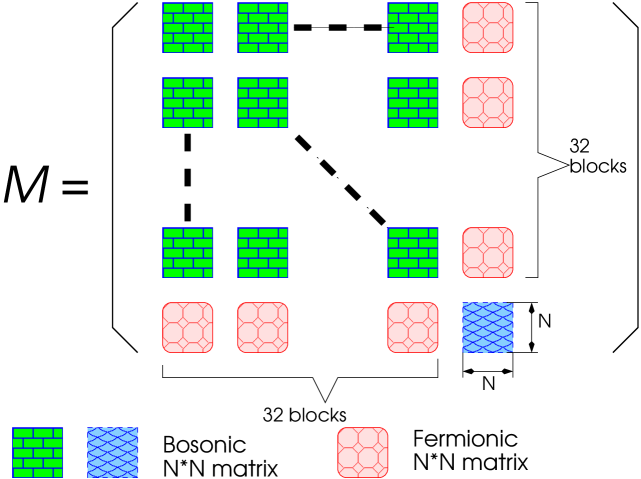
  Figure 9: The way large $N$ matrices are embedded in this matrix model.

• The commutator in (4.32) is taken with respect to the $N\times N$ matrices, rather than the $33\times 33$ supermatrices.

• The traces with respect to $32\times 32$ matrices and $N\times N$ large matrices are confusing. Throughout in this paper we use

  • $Tr$ as a trace of $N\times N$ large matrices.

  • $tr$ as a trace of $32\times 32$ matrices, and $Str$ as a supertrace of $33\times 33$ matrices.

  We do not necessarily write explicitly the size of the matrices.

• It is often convenient to utilize the representation of color indices of $su(N)$ Lie algebra. Each component ${M_{P}}^{Q}$, now promoted to a $N\times N$ matrix, is expanded by the basis of the generators of $SU(N)$ Lie group as follows:

  $${M_{P}}^{Q}=\sum_{a=1}^{N^{2}}{(M^{a})_{P}}^{Q}T^{a},$$ (4.34)

  where ${(M^{a})_{P}}^{Q}$ are c-number coefficients of the expansion with respect to the generators $\{T^{a}\}$. Since the commutator is taken with respect to $N\times N$ hermitian matrices, it is easy to see that the action is rewritten as (4.32) by the representation of the color indices. And the expression in terms of the structure constant is (4.33), noting that $Tr(T^{a}[T^{b},T^{c}])=\frac{i}{2}f^{abc}$.

• This matrix model possesses no free parameter. This property is easier to see than in IKKT model. The parameter $g$ is absorbed in the supermatrices $M$ only by the scale redefinition $M\rightarrow g^{\frac{2}{3}}M$.

• It is indispensable to multiply the overall $i$ so that the action should be a real quantity, because $Tr(T^{a}[T^{b},T^{c}])=\frac{i}{2}f^{abc}$, where the structure constant is a real number. We require the action to be real because of the analog of quantum field theory. In considering the quantum field theory in Minkowski space, we usually consider the action to be real so that the Hamiltonian of the theory is an hermitian object.

This model apparently possesses the following pathological properties [13]. The first is that this theory is not bounded from above or below. This pathology stems from the fact that the action is cubic, and can be seen by a naive field redefinition $M\rightarrow M\lambda$. The action is rewritten as $I=\frac{i\lambda^{3}}{g^{2}}Tr_{N\times N}({M_{p}}^{Q}[{M_{Q}}^{R},{M_{R}}^{p}]-{M_{33}}^{Q}[{M_{Q}}^{R},{M_{R}}^{33}])$, and we can set this action to be $I\to\pm\infty$ by setting the parameter to be $\lambda\to\pm\infty$. This means that the path integral of the theory $S=\int e^{-I}$ does not converge. However, note that this pathology is shared by general relativity. This pathological property of general relativity can be seen by Weyl transformation

$$I_{einstein}=\int d^{d}x\sqrt{g}R=\int d^{d}xe^{(\frac{d}{2}-1)\omega}\sqrt{g}(R-(d-1)\nabla^{2}\omega-\frac{(d-2)(d-1)}{4}\partial_{\mu}\omega\partial^{\mu}\omega).$$

Although the pathology of Smolin’s proposal is not a happy aspect, this may be regarded as a good news because this may indicate that Smolin’s proposals may include general relativity by taking a due limit. The second problem is that this theory possesses no explicit time coordinate. This is again a pathology shared by general relativity. We can introduce a time coordinate by expanding the theory around a certain background. Once a time coordinate is introduced, we can construct a Hamiltonian of this theory. We will investigate the compactification later.

4.2.1 Supertrace

We have seen in (4.32) that this cubic action is described by the supertrace. Let us give a brief explanation of the notion of supertrace for general supermatrices. A supertrace is defined as

$$Str_{33\times 33}M\stackrel{{\scriptstyle def}}{{=}}(\sum_{p=1}^{32}{M_{p}}^{p})-{M_{33}}^{33}.$$ (4.35)

Note that the last bosonic part is subtracted, rather than summed. In other words, when the supermatrix is expressed by $M=\left(\begin{array}[]{cc}m&\psi\\ i{\bar{\phi}}&v\end{array}\right)$, the supertrace is

$$StrM=(tr_{32\times 32}m)-v.$$ (4.36)

The supertrace of the supermatrices guarantees the cyclic rule. This property can be verified by the following argument. We consider two arbitrary matrices:

$$Z_{1}=\left(\begin{array}[]{cc}A_{11}&\alpha_{12}\\ \alpha^{T}_{21}&a_{22}\end{array}\right),\hskip 8.53581ptZ_{2}=\left(\begin{array}[]{cc}B_{11}&\beta_{12}\\ \beta^{T}_{21}&b_{22}\end{array}\right),$$ (4.41)

where $A_{11}$ and $B_{11}$ are 32 $\times$ 32 bosonic matrices, $\alpha_{12}$ , $\alpha_{21}$ , $\beta_{12}$ and $\beta_{21}$ are 32-component fermionic vectors, and $a_{22}$ and $b_{22}$ are c-numbers. We consider the supertrace of $Z_{1}Z_{2}$ and $Z_{2}Z_{1}$:

$$Str(Z_{1}Z_{2})=tr(A_{11}B_{11}+\alpha_{12}\beta^{T}_{21})-(\alpha^{T}_{21}\beta_{12}+a_{22}b_{22}),$$ (4.42)

$$Str(Z_{2}Z_{1})=tr(A_{11}B_{11}+\beta_{12}\alpha^{T}_{21})-(\beta^{T}_{21}\alpha_{12}+a_{22}b_{22}).$$ (4.43)

Since $\alpha$ and $\beta$ are fermionic quantities, the sign changes if we change the order. Therefore, we establish that it is not an ordinary trace but a supertrace that the cyclic rule $Str(Z_{1}Z_{2})=Str(Z_{2}Z_{1})$ holds true of the supermatrix.

4.2.2 Gauge Symmetry

Let us investigate the gauge symmetry of this cubic action. We have reviewed in the previous section that the gauge group of IKKT model is $SO(9,1)\times SU(N)$. The same is true of the promotion of this cubic matrix model from the c-number elements of $osp(1|32,R)$ multiplets to hermitian $N\times N$ matrices. The gauge group of this cubic matrix model is $OSp(1|32,R)\times SU(N)$. This means that the generator ${\cal X}$ of this gauge group is:

$${\cal X}=(X\otimes{\bf 1}_{N\times N})+({\bf 1}_{33\times 33}\otimes u),\textrm{ with }X\in osp(1|32,R)\textrm{ and }u\in su(N),$$ (4.44)

with the tensor product $\otimes$ taken with respect to two matrices. Therefore, like IKKT model, the gauge transformation with respect to the $osp(1|32,R)$ Lie algebra and $su(N)$ Lie algebra is taken independently. The gauge transformation with respect to $su(N)$ Lie algebra is the same as the conventional proposal for large $N$ reduced models, and we do not repeat it. On the other hand, the gauge invariance of $su(N)$ transformation teaches us the physical significance of taking the supertrace with respect to $33\times 33$ supermatrices. The infinitesimal gauge transformation is of course

$$\textrm{For an arbitrary element of }u\in osp(1|32,R),\textrm{ the gauge transformation is }M\rightarrow M+[u,M].$$ (4.45)

This indicates that the gauge invariance becomes possible only if the action possesses the cyclic symmetry. As we have investigated before, the cyclic symmetry for the supermatrix is guaranteed not for the ordinary trace but the supertrace. Therefore, it is indispensable to take the supertrace with respect to the supermatrix if we are to construct a physically consistent theory.

4.2.3 Explicit Form of the Action

When we analyze this matrix theory, it is convenient to express this action in terms of the components of $osp(1|32,R)$ group $M=\left(\begin{array}[]{cc}m&\psi\\ i{\bar{\psi}}&0\end{array}\right)$. The computation is easier to perform if we regard the components of $32\times 32$ matrices as a c-number utilizing (4.33).

$$Str(M^{a}M^{b}M^{c})$$ (4.46)

$$= tr({(m^{a})_{p}}^{q}{(m^{b})_{q}}^{r}{(m^{c})_{r}}^{p})+itr({(m^{a})_{p}}^{q}(\psi^{b})_{q}{(\bar{\psi}^{c})}^{p})+itr((\psi^{a})_{p}{(\bar{\psi}^{b})}^{q}{(m^{c})_{q}}^{p})-i{(\bar{\psi}^{a})}^{q}{(m^{b})_{q}}^{r}(\psi^{c})_{r}$$

$$\stackrel{{\scriptstyle\ast}}{{=}} tr({(m^{a})_{p}}^{q}{(m^{b})_{q}}^{r}{(m^{c})_{r}}^{p})-itr({(\bar{\psi}^{c})}^{p}{(m^{a})_{p}}^{q}(\psi^{b})_{q})-itr({(\bar{\psi}^{b})}^{q}{(m^{c})_{q}}^{p}(\psi^{a})_{p})-i{(\bar{\psi}^{a})}^{q}{(m^{b})_{q}}^{r}(\psi^{c})_{r}$$

$$= tr(m^{a}m^{b}m^{c})-3i{\bar{\psi}^{a}}m^{b}\psi^{c}.$$

In the equality $\stackrel{{\scriptstyle\ast}}{{=}}$, we utilized the cyclic symmetry of the $32\times 32$ trace. However there is a important point in treating fermionic quantities. Since a fermion has jumped over another fermions in the cyclic procedure, the sign must change in the cyclic rule. Therefore, the action of this matrix model is rewritten as

$$I=-\frac{f_{abc}}{2g^{2}}(tr(m^{a}m^{b}m^{c})-3i{\bar{\psi}^{a}}m^{b}\psi^{c})=\frac{i}{g^{2}}Tr({m_{p}}^{q}[{m_{q}}^{r},{m_{r}}^{p}])-3i{\bar{\psi}}[m,\psi]).$$ (4.47)

The former is equivalent to the latter, the former written in terms of the color index and the latter adopting the large $N$ matrix representation. From now on, we express the bosonic $32\times 32$ matrices in terms of the basis of 11 dimensional gamma matrices:

$$m=u_{\mu_{1}}\Gamma^{\mu_{1}}+\frac{1}{2}u_{\mu_{1}\mu_{2}}\Gamma^{\mu_{1}\mu_{2}}+\frac{1}{5!}u_{\mu_{1}\cdots\mu_{5}}\Gamma^{\mu_{1}\cdots\mu_{5}}.$$ (4.48)

The computation of the bosonic cubic terms in terms of this representation is a bit tedious, but it is worth while to overcome this obstacle because the physics described by this matrix model can be understood more transparently if we consider the theory in terms of 11 dimensional framework. Originally, $osp(1|32,R)$ super Lie algebra is known as an ’ultimate symmetry of M-theory’, and the 11 dimensional representation of $osp(1|32,R)$ super Lie algebra is the best description to investigate the physics of unified superstring theory.

Our problem in this paper is the correspondence between our cubic matrix model and the existing 10 dimensional matrix theories, such as IKKT model. For this purpose, it is more convenient to express the induces for 10 dimensions, and we introduce the following new variables.

$$Z=u,\hskip 8.53581ptW=u_{\sharp},\hskip 8.53581ptA^{(\pm)}_{i}=u_{i}\pm u_{i\sharp},\hskip 8.53581ptC_{i_{1}i_{2}}=u_{i_{1}i_{2}},\hskip 8.53581ptD_{i_{1}i_{2}}=u_{i_{1}i_{2}\sharp},\hskip 8.53581pt$$

$$E^{(\pm)}_{i_{1}i_{2}i_{3}}=u_{i_{1}i_{2}i_{3}}\pm u_{i_{1}i_{2}i_{3}\sharp},\hskip 8.53581ptG_{i_{1}\cdots i_{4}}=u_{i_{1}\cdots i_{4}},\hskip 8.53581ptH_{i_{1}\cdots i_{4}}=u_{i_{1}\cdots i_{4}\sharp},\hskip 8.53581ptI^{(\pm)}_{i_{1}\cdots i_{5}}=\frac{1}{2}(u_{i_{1}\cdots i_{5}}\pm{\tilde{u}}_{i_{1}\cdots i_{5}}).$$ (4.49)

• The indices $i_{1},i_{2},\cdots$ runs $0,1,\cdots,9$, excluding the $x^{\sharp}$ direction. Throughout this paper, $\sharp$ denotes the 10th direction.

• On the other hand, the conventional induces $\mu,\nu,\cdots$ runs $0,1,\cdots,9,\sharp$.

• The quantity ${\tilde{u}}_{i_{1}\cdots i_{5}}$ denotes the dual of $u_{i_{1}\cdots i_{5}}$:

  $${\tilde{u}}_{i_{1}\cdots i_{5}}\stackrel{{\scriptstyle def}}{{=}}\frac{-1}{5!}u_{i_{6}\cdots i_{10}}\epsilon^{i_{1}\cdots i_{10}\sharp}.$$ (4.50)

  The quantities $I^{(+)}_{i_{1}\cdots i_{5}}$ and $I^{(-)}_{i_{1}\cdots i_{5}}$ are defined to be self-dual and anti-self-dual, respectively:

  $$I^{(+)}_{i_{1}\cdots i_{5}}={\tilde{I}}^{(+)}_{i_{1}\cdots i_{5}},\hskip 8.53581ptI^{(-)}_{i_{1}\cdots i_{5}}=-{\tilde{I}}^{(-)}_{i_{1}\cdots i_{5}}.$$ (4.51)

• Since we are considering $osp(1|32,R)$ matrix model, only the variables $W$, $A^{(\pm)}_{i}$, $C_{i_{1}i_{2}}$, $H_{i_{1}\cdots i_{4}}$ and $I^{(\pm)}_{i_{1}\cdots i_{5}}$ concerns the discussion in this section. However, we introduce the variables of other ranks for future reference.

These new variables see other spacetime directions than the 10th direction. We give the direction $x^{\sharp}$ a special treatment because we would like to preserve the Lorentz symmetry of the 10 dimensional description. Utilizing these variables, and adopting the formulation of $N\times N$ matrices, this action is computed to be

$$I_{b} = \frac{i}{g^{2}}Tr_{N\times N}(-96[A^{(+)}_{i_{1}},A^{(-)}_{i_{2}}]C^{i_{1}i_{2}}-96W[A^{(+)i},A^{(-)}_{i}]+\frac{4}{5}W[I^{(+)}_{i_{1}\cdots i_{5}},I^{(-)i_{1}\cdots i_{5}}]$$ (4.52)

$$- 4H_{i_{1}\cdots i_{4}}([A^{(+)}_{i_{5}},I^{(-)i_{1}\cdots i_{5}}]-[A^{(-)}_{i_{5}},I^{(+)i_{1}\cdots i_{5}}])-8C_{i_{1}i_{2}}[{I^{(+)i_{1}}}_{i_{3}\cdots i_{6}},I^{(-)i_{2}\cdots i_{6}}]$$

$$+ \frac{8}{3}{H^{jk}}_{i_{1}i_{2}}([{I^{(+)}}_{jki_{3}i_{4}i_{5}},I^{(-)i_{1}\cdots i_{5}}]-[{I^{(-)}}_{jki_{3}i_{4}i_{5}},I^{(+)i_{1}\cdots i_{5}}])$$

$$+ 32[{C^{i_{1}}}_{i_{2}},C_{i_{1}i_{3}}]C^{i_{2}i_{3}}-16C_{i_{1}i_{2}}[{H^{i_{1}}}_{i_{3}i_{4}i_{5}},H^{i_{2}\cdots i_{5}}]+\frac{1}{27}H_{i_{1}\cdots i_{4}}[{H^{j}}_{i_{5}\cdots i_{7}},H_{ji_{8}i_{9}i_{10}}]\epsilon^{i_{1}\cdots i_{10}\sharp}),$$

$$I_{f} = \frac{i}{g^{2}}Tr_{N\times N}(-3i(-{\bar{\psi}_{L}}[W,\psi_{R}]+{\bar{\psi}_{R}}[W,\psi_{L}])-3i({\bar{\psi}_{L}}\Gamma^{i}[A^{(+)}_{i},\psi_{L}]+{\bar{\psi}_{R}}\Gamma^{i}[A^{(-)}_{i},\psi_{R}])$$ (4.53)

$$- \frac{3i}{2!}({\bar{\psi}_{L}}\Gamma^{i_{1}i_{2}}[C_{i_{1}i_{2}},\psi_{R}]+{\bar{\psi}_{R}}\Gamma^{i_{1}i_{2}}[C_{i_{1}i_{2}},\psi_{L}])-\frac{3i}{4!}(-{\bar{\psi}_{L}}\Gamma^{i_{1}i_{2}i_{3}i_{4}}[H_{i_{1}i_{2}i_{3}i_{4}},\psi_{R}]+{\bar{\psi}_{R}}\Gamma^{i_{1}i_{2}i_{3}i_{4}}[H_{i_{1}i_{2}i_{3}i_{4}},\psi_{L}])$$

$$- \frac{3i}{5!}(2{\bar{\psi}_{L}}\Gamma^{i_{1}i_{2}i_{3}i_{4}i_{5}}[{I^{(+)}}_{i_{1}i_{2}i_{3}i_{4}i_{5}},\psi_{L}]+2{\bar{\psi}_{R}}\Gamma^{i_{1}i_{2}i_{3}i_{4}i_{5}}[{I^{(-)}}_{i_{1}i_{2}i_{3}i_{4}i_{5}},\psi_{R}])),$$

where $I_{b}$ and $I_{f}$ are the bosonic and fermionic parts of the action $I$, respectively. The whole action is $I=I_{b}+I_{f}$. The computation of this action is lengthy, and we refer the proof to Appendix. B.2.

4.3 Identification of SUSY with IKKT Model

We next investigate the SUSY of this cubic matrix model. The SUSY of the theory is an essential property because this symmetry gives a wealth of information about the theory. As we have seen in the previous section, IKKT model shares ${\cal N}=2$ SUSY with type IIB superstring theory, and this SUSY teaches us a lot about the properties of IKKT model. For example, the ${\cal N}=2$ SUSY indicates the existence of massless graviton, which is an essential property for a theory including gravity.

The investigation of the SUSY of this cubic matrix model is an interesting issue to be acquainted with the properties of this theory. Azuma, Iso, Kawai and Ohwashi [1] pointed out that this cubic matrix model possesses ${\cal N}=2$ SUSY to be identified with that of IKKT model. The discovery of the existence of ${\cal N}=2$ is of significance in that they discovered the property shared by the existing matrix model.

One of the motivation of tackling with this cubic matrix is to investigate a matrix model which naturally contains the existing proposal for the constructive definition of superstring, such as IKKT or BFSS model. That the $osp(1|32,R)$ cubic model may contain these models is conjectured from the group theoretical consideration of $osp(1|32,R)$ super Lie algebra. Performing the dimensional reduction on the 11 dimensional representation into the 10 dimensional representation, we obtain a symmetry of both type IIA and type IIB [15]. The work [1] solidified the belief that this cubic matrix model naturally includes IKKT model by the identification of the ${\cal N}=2$ SUSY with that of IKKT model (3.35) and (3.36).

4.3.1 Definition of Supercharge

First, let us consider what is the SUSY of this cubic matrix model. The SUSY is a symmetry relating the fermions and the bosons : a SUSY transformation turns a bosonic state into a fermionic state and vice versa. Let $Q$ be an operator which generates such transformations $Q$ is called a supercharge, and this satisfies

$$Q|\textrm{Boson}\rangle=|\textrm{Fermion}\rangle,\hskip 8.53581ptQ|\textrm{Fermion}\rangle=|\textrm{Boson}\rangle.$$ (4.54)

A supercharge must be therefore a fermionic quantity, and there is no room for the fermionic fields to enter the supercharge. Then, we define a supercharge of this cubic matrix theory as follows:

$$Q=\left(\begin{array}[]{cc}0&\chi\\ i{\bar{\chi}}&0\end{array}\right).$$ (4.57)

Originally, the supercharge must satisfy the Haag-Lopuszanski-Sohnius extension of Coleman-Mandula theorem, as we have mentioned in the previous chapter (3.37). However, we have yet to understand the meaning of the translation of the bosonic fields in this cubic matrix theory. And it is impossible to justify here that the definition (4.57) is an eligible supercharge. We defer this argument later, and we consider the justification of this SUSY transformation by comparing this ’SUSY’ transformation with that of IKKT model.

4.3.2 ${\cal N}=2$ SUSY transformation

We consider the ’SUSY’ transformations by the above supercharge (4.57). The SUSY transformation of this model is expressed by the infinitesimal transformation by this supercharge. For a matter field of this supermatrix theory $M=\left(\begin{array}[]{cc}m&\psi\\ i{\bar{\psi}}&0\end{array}\right)$, the SUSY transformation $\delta_{\chi}M$ is the commutator with the supercharge:

$$\delta_{\chi}M=[Q,M]=[\left(\begin{array}[]{cc}0&\chi\\ i{\bar{\chi}}&0\end{array}\right),\left(\begin{array}[]{cc}m&\psi\\ i{\bar{\psi}}&0\end{array}\right)]=\left(\begin{array}[]{cc}i(\chi{\bar{\psi}}-\psi{\bar{\chi}})&-m\chi\\ i{\bar{\chi}}m&0\end{array}\right).$$ (4.64)

There is another kind of supersymmetry in this cubic matrix theory. Note that the action of this matrix theory (4.32) includes the commutators. This means that this cubic matrix theory is invariant under a naive translation of the fermionic field $\psi\rightarrow\psi+\epsilon$. This is the same situation as emerged in the case of IKKT model, where the fermionic field emerged only as a commutator with the matter field.

The notion of ’homogeneous’ and ’inhomogeneous’ SUSY transformations is used in the same sense as in IKKT model.

• The former SUSY, the infinitesimal transformation by the supercharge, is called homogeneous SUSY, and we use $\delta^{(1)}_{\chi}$ to represent this homogeneous SUSY by the supercharge $Q_{\chi}=\left(\begin{array}[]{cc}0&\chi\\ i{\bar{\chi}}&0\end{array}\right)$.

• The latter SUSY is called inhomogeneous SUSY. $\delta^{(2)}_{\epsilon}$ is defined as the inhomogeneous SUSY with the translation of the fermion $\psi\rightarrow\psi+\epsilon$.

We have discerned that this cubic matrix model possesses ${\cal N}=2$ SUSY in the same sense as IKKT model. This stems from the fact that the action is written by the commutator of the matrices. The SUSY of the $osp(1|32,R)$ cubic matrix model is summarized as

• homogeneous: $\delta^{(1)}_{\chi}m=i(\chi{\bar{\psi}}-\psi{\bar{\chi}})$ , $\delta^{(2)}_{\epsilon}\psi=-m\chi$.

• inhomogeneous : $\delta^{(2)}_{\epsilon}m=0$, $\delta^{(2)}_{\epsilon}\psi=\epsilon$.

We have seen that this cubic model possesses ${\cal N}=2$ SUSY, and the origin of the homogeneous and the inhomogeneous SUSY is similar to the case of the IKKT model. However, there are two questions in order to solidify the correspondence of the SUSY of the cubic matrix model with that of IKKT model. One question stems from the discrepancy of the number of the SUSY parameters between the cubic model and IKKT model. This cubic matrix model possesses twice as many SUSY parameters as IKKT model. The SUSY parameter of the homogeneous SUSY in IKKT model is 10 dimensional Majorana-Weyl spinors, and the number of the spinors are 16. On the other hand, The SUSY parameter of the inhomogeneous SUSY, id est the naive translation, is also 16. Therefore, IKKT model possesses in total 32 SUSY parameter. On the other hand, our cubic model possesses 32 homogeneous SUSY parameters $\chi$ and 32 inhomogeneous SUSY parameters $\epsilon$, in total 64 SUSY parameters. In order to identify the SUSY of the cubic matrix model with that of IKKT model, it seem to be necessary to divide the SUSY parameter into two groups each of which consists of 32 fermions. Another issue to tackle with is the identification of the fields of the cubic matrix model with those of IKKT model. We investigate this issue through the SUSY transformation on the fields of the matter fields. This issue is interesting in the light of not only the identification of the supersymmetry but also in that this question provides us with the clues of what fields we should regard as the fundamental fields.

The clue to the first question lies in the chiral decomposition of the fermionic fields. We separate 64 fermionic SUSY parameters into the group of left and right chirality, and thus divide these 64 SUSY parameters into two groups. We have introduced the definition of the chiral projection in Appendix. A.2.1. We define a homogeneous SUSY transformation $\delta^{(1)}_{\chi_{L}}$ and $\delta^{(1)}_{\chi_{R}}$ as the transformation by the supercharge $Q_{\chi_{L}}$ and $Q_{\chi_{R}}$ respectively:

$$Q_{\chi_{L}}=\left(\begin{array}[]{cc}0&\chi_{L}\\ i{\bar{\chi}_{L}}&0\end{array}\right),\hskip 8.53581ptQ_{\chi_{R}}=\left(\begin{array}[]{cc}0&\chi_{R}\\ i{\bar{\chi}_{R}}&0\end{array}\right).$$ (4.69)

Likewise, the inhomogeneous SUSY transformation $\delta^{(2)}_{\epsilon_{L,R}}$ as the translation of the fermions:

$$\delta^{(2)}_{\epsilon_{L.R}}\psi=\epsilon_{L.R}.$$ (4.70)

We next pursue the problem of how each of the components of the matter fields

$$m = W\Gamma^{\sharp}+\frac{1}{2}A^{(+)}_{i}\Gamma^{i}(1+\Gamma^{\sharp})+\frac{1}{2}A^{(-)}_{i}\Gamma^{i}(1-\Gamma^{\sharp})+\frac{1}{2!}C_{i_{1}i_{2}}\Gamma^{i_{1}i_{2}}+\frac{1}{4!}H_{i_{1}\cdots i_{4}}\Gamma^{i_{1}\cdots i_{4}}$$ (4.71)

$$+ \frac{1}{5!}I^{(+)}_{i_{1}\cdots i_{5}}\Gamma^{i_{1}\cdots i_{5}}(1+\Gamma^{\sharp})+\frac{1}{5!}I^{(-)}_{i_{1}\cdots i_{5}}\Gamma^{i_{1}\cdots i_{5}}(1-\Gamma^{\sharp})$$

are transformed under this SUSY transformation. We have verified that the commutator of the homogeneous and inhomogeneous SUSY transformation gives a nonvanishing contribution. In extracting the SUSY transformation of each of $W$, $A^{(\pm)}_{i}$, $C_{i_{1}i_{2}}$, $H_{i_{1}\cdots i_{4}}$ and $I^{(\pm)}_{i_{1}\cdots i_{5}}$, we use the technique introduced in Appendix. A.2.6. We find it a natural interpretation to regard the fields of rank 1 as identified with the fields of IKKT model.

The homogeneous SUSY transformation is computed as follows. We would like to extract from the SUSY transformation $\delta^{(1)}_{\chi}m=i(\chi{\bar{\psi}}-\psi{\bar{\chi}})$ the transformations of the fields $A^{(+)}_{i}$ and $B^{(+)}_{i}$. We utilize the formulae in Appendix. A.2.6 to extract the SUSY transformation for these fields. Utilizing the formulae (A.32), we obtain

$$\delta^{(1)}_{\chi}A^{(+)}_{i} = \frac{1}{32}tr((\delta^{(1)}_{\chi}m)\Gamma_{i})+\frac{-1}{32}tr((\delta^{(1)}_{\chi}m)\Gamma_{i\sharp})=\frac{i}{32}tr((\chi{\bar{\psi}}-\psi{\bar{\chi}})\Gamma_{i}(1-\Gamma_{\sharp})$$ (4.72)

$$= \frac{i}{32}(-{\bar{\psi}}\Gamma_{i}(1-\Gamma_{\sharp})\chi+{\bar{\chi}}\Gamma_{i}(1-\Gamma_{\sharp})\psi)=\frac{i}{16}({\bar{\chi}}\Gamma_{i}(1-\Gamma_{\sharp})\psi)=\frac{i}{8}{\bar{\chi}_{R}}\Gamma_{i}\psi_{R},$$

$$\delta^{(1)}_{\chi}A^{(-)}_{i} = \frac{1}{32}tr((\delta^{(1)}_{\chi}m)\Gamma_{i})-\frac{-1}{32}tr((\delta^{(1)}_{\chi}m)\Gamma_{i\sharp})=\frac{i}{8}{\bar{\chi}_{L}}\Gamma_{i}\psi_{L},$$ (4.73)

$$\delta^{(1)}_{\chi}\psi = -m\chi.$$ (4.74)

$\delta^{(1)}_{\chi}A^{(-)}_{i}$ is computed in the same manner as $\delta^{(1)}_{\chi}A^{(+)}_{i}$. These transformation laws of the fields possesses the same structure as the homogeneous SUSY transformation of IKKT model. Now, we have discerned the correspondence between the bosonic fields and the fermionic fields.

bosons $A_{i}$ (IKKT)	fermions $\psi$(IKKT)
$A^{(+)}_{i}$	$\psi_{R}=\frac{1-\Gamma^{\sharp}}{2}\psi$
$A^{(-)}_{i}$	$\psi_{L}=\frac{1+\Gamma^{\sharp}}{2}\psi$

4.3.3 Commutation relation of SUSY transformation

We next consider the commutation relation of the SUSY transformations. In IKKT model, we have seen the commutators of the supersymmetries (3.20), (3.21) and (3.22). We wish to find the same structure in the cubic matrix model. We investigate the commutators of the SUSY transformations for each chirality

$$(1)[\delta^{(1)}_{\chi},\delta^{(1)}_{\epsilon}]A^{(\pm)}_{i},\hskip 8.53581pt(2)[\delta^{(2)}_{\chi},\delta^{(2)}_{\epsilon}]A^{(\pm)}_{i},\hskip 8.53581pt(3)[\delta^{(1)}_{\chi},\delta^{(2)}_{\epsilon}]A^{(\pm)}_{i}.$$ (4.75)

As we have reviewed in the previous chapter, these commutation relations reveal what is the translation of the bosonic vector fields, and served to examine that the ${\cal N}=2$ SUSY transformations satisfy Haag-Lopuszanski-Sohnius theorem $\{Q,Q\}=P_{i}=$ (translation of bosonic fields). The investigation of the commutators is an important problem in this cubic matrix model, too. And we investigate these commutators one by one. It is a trivial matter that the commutator (2) vanishes because the inhomogeneous SUSY transformation is just a naive translation of the fermions, and we investigate the rest of the SUSY transformations.

SUSY transformation $(3)[\delta^{(1)}_{\chi},\delta^{(2)}_{\epsilon}]A^{(\pm)}_{i}$

.
Even though the order is upside down, let us investigate the SUSY of this type. In IKKT model, this is the only nonvanishing commutator, and this commutation relation would give us a big information about the correspondence of the SUSY between the cubic model and IKKT model. In our cubic model, this commutation relation is obtained by

$$[\delta^{(1)}_{\chi},\delta^{(2)}_{\epsilon}]m=-i(\chi{\bar{\epsilon}}-\epsilon{\bar{\chi}}),\hskip 8.53581pt[\delta^{(1)}_{\chi},\delta^{(2)}_{\epsilon}]\psi=0.$$ (4.76)

(Proof) We perform the similar procedure, as in the case of IKKT model. In considering the commutator of $[\delta^{(1)}_{\chi},\delta^{(2)}_{\epsilon}]$, it is convenient to compare the two paths of the SUSY transformations.

• $m\stackrel{{\scriptstyle\delta^{(2)}_{\epsilon}}}{{\to}}m\stackrel{{\scriptstyle\delta^{(1)}_{\chi}}}{{\to}}m+i(\chi{\bar{\psi}}-\psi{\bar{\chi}})$, whereas $m\stackrel{{\scriptstyle\delta^{(1)}_{\chi}}}{{\to}}m+i(\chi{\bar{\psi}}-\psi{\bar{\chi}})\stackrel{{\scriptstyle\delta^{(2)}_{\epsilon}}}{{\to}}m+i\chi({\bar{\psi}}+{\bar{\epsilon}})-i(\psi+\epsilon){\bar{\chi}}$.

• $\psi\stackrel{{\scriptstyle\delta^{(2)}_{\epsilon}}}{{\to}}\psi+\epsilon\stackrel{{\scriptstyle\delta^{(1)}_{\chi}}}{{\to}}\psi+\epsilon-m\chi$, whereas $\psi\stackrel{{\scriptstyle\delta^{(1)}_{\chi}}}{{\to}}\psi-m\chi\stackrel{{\scriptstyle\delta^{(2)}_{\epsilon}}}{{\to}}\psi+\epsilon-m\chi$.

Taking the difference of these two paths for the bosonic fields and the fermions respectively, we obtain the above commutation relation. (Q.E.D.)

We extract the commutators of the SUSY transformation with respect to the fields of rank 1: $A^{(\pm)}_{i}$. For this purpose, we make use of the formulae in Appendix. A.2.6, in the same fashion as in the homogeneous SUSY transformation itself:

$$[\delta^{(1)}_{\chi},\delta^{(2)}_{\epsilon}]A^{(+)}_{i}=\frac{1}{32}tr(([\delta^{(1)}_{\chi},\delta^{(2)}_{\epsilon}]m)\Gamma_{i})+\frac{-1}{32}tr(([\delta^{(1)}_{\chi},\delta^{(2)}_{\epsilon}]m)\Gamma_{i\sharp})=\frac{i}{32}tr((\epsilon{\bar{\chi}}-\chi{\bar{\epsilon}})\Gamma_{i}(1-\Gamma_{\sharp}))$$

$$\hskip 62.59605pt=\frac{i}{32}(-{\bar{\chi}}\Gamma_{i}(1-\Gamma_{\sharp})\epsilon+{\bar{\epsilon}}\Gamma_{i}(1-\Gamma_{\sharp})\chi)=\frac{i}{16}{\bar{\epsilon}}\Gamma_{i}(1-\Gamma_{\sharp})\chi=\frac{i}{8}{\bar{\epsilon}}_{R}\Gamma_{i}\chi_{R},$$ (4.77)

$$[\delta^{(1)}_{\chi},\delta^{(2)}_{\epsilon}]A^{(-)}_{i}=\frac{1}{32}tr(([\delta^{(1)}_{\chi},\delta^{(2)}_{\epsilon}]m)\Gamma_{i})-\frac{-1}{32}tr(([\delta^{(1)}_{\chi},\delta^{(2)}_{\epsilon}]m)\Gamma_{i\sharp})=\frac{i}{8}{\bar{\epsilon}}_{L}\Gamma_{i}\chi_{L}.$$ (4.78)

Extracting the specific chirality of the SUSY parameters, the nonvanishing commutators are now clear:

$$[\delta^{(1)}_{\chi_{L}},\delta^{(2)}_{\epsilon_{L}}]A^{(+)}_{i}=0,\hskip 42.67912pt[\delta^{(1)}_{\chi_{R}},\delta^{(2)}_{\epsilon_{R}}]A^{(+)}_{i}=\frac{i}{8}{\bar{\epsilon}}_{R}\Gamma_{i}\chi_{R},$$

$$[\delta^{(1)}_{\chi_{L}},\delta^{(2)}_{\epsilon_{L}}]A^{(-)}_{i}=\frac{i}{8}{\bar{\epsilon}}_{L}\Gamma_{i}\chi_{L},\hskip 8.53581pt[\delta^{(1)}_{\chi_{R}},\delta^{(2)}_{\epsilon_{R}}]A^{(-)}_{i}=0.$$ (4.79)

The commutators with different chirality of the two SUSY parameters clearly vanishes:

$$[\delta^{(1)}_{\chi_{L}},\delta^{(2)}_{\epsilon_{R}}]A^{(\pm)}_{i}=[\delta^{(1)}_{\chi_{R}},\delta^{(2)}_{\epsilon_{L}}]A^{(\pm)}_{i}=0.$$ (4.80)

These combinations of SUSY transformations clearly resemble the structure of the SUSY transformations of IKKT model. And the correspondence between the vector fields and the chirality of the fermionic fields matches that obtained by the correspondence of the homogeneous transformation itself.

SUSY transformation $(1)[\delta^{(1)}_{\chi},\delta^{(1)}_{\epsilon}]A^{(\pm)}_{i}$

.
In the case of IKKT model, this SUSY transformation vanishes up to the gauge transformation, as we have seen in (3.20). We want to find the same vanishing in our cubic model, if we are to identify the SUSY transformation. However, it turns out that this commutator does not vanish. In investigating this commutation relation, it is easier to utilize the following identity:

$$[\delta^{(1)}_{\chi},\delta^{(1)}_{\epsilon}]M=[[Q_{\chi},Q_{\epsilon}],M].$$ (4.81)

This can be verified by the explicit computation of the both hand sides:

$$[\delta^{(1)}_{\chi},\delta^{(1)}_{\epsilon}]M=[Q_{\chi},[Q_{\epsilon},M]]-[Q_{\epsilon},[Q_{\chi},M]]$$

$$\hskip 28.45274pt=Q_{\chi}Q_{\epsilon}M-Q_{\chi}MQ_{\epsilon}-Q_{\epsilon}MQ_{\chi}+MQ_{\epsilon}Q_{\chi}-Q_{\epsilon}Q_{\chi}M+Q_{\chi}MQ_{\epsilon}+Q_{\epsilon}MQ_{\chi}-MQ_{\chi}Q_{\epsilon}=[[Q_{\chi},Q_{\epsilon}],M].$$

This commutator of the SUSY transformation is thus obtained by

$$[\delta^{(1)}_{\chi},\delta^{(1)}_{\epsilon}]M=[\left(\begin{array}[]{cc}i(\chi{\bar{\epsilon}}-\epsilon{\bar{\chi}})&0\\ 0&0\end{array}\right),\left(\begin{array}[]{cc}m&\psi\\ i{\bar{\psi}}&0\end{array}\right)]=\left(\begin{array}[]{cc}[i(\chi{\bar{\epsilon}}-\epsilon{\bar{\chi}}),m]&i(\chi{\bar{\epsilon}}-\epsilon{\bar{\chi}})\psi\\ -i{\bar{\psi}}(\chi{\bar{\epsilon}}-\epsilon{\bar{\chi}})&0\end{array}\right).$$ (4.88)

This relation reveals that the commutators of the two homogeneous transformation are

$$[\delta^{(1)}_{\chi},\delta^{(1)}_{\epsilon}]m=i[(\chi{\bar{\epsilon}}-\epsilon{\bar{\chi}}),m],$$ (4.89)

$$[\delta^{(1)}_{\chi},\delta^{(1)}_{\epsilon}]\psi=i(\chi{\bar{\epsilon}}-\epsilon{\bar{\chi}})\psi.$$ (4.90)

We have seen in (4.79) which chiralities of the SUSY parameters correspond to the vector fields $A^{(\pm)}_{i}$. According to this correspondence, we examine the commutation relation with respect to the following cases.

We first investigate the commutation relation $[\delta^{(1)}_{\chi_{L}},\delta^{(1)}_{\epsilon_{L}}]$. We examine this commutation relation of this SUSY transformation:

$$[\delta^{(1)}_{\chi_{L}},\delta^{(1)}_{\epsilon_{L}}]A^{(-)}_{i}=\frac{1}{32}tr(([\delta^{(1)}_{\chi_{L}},\delta^{(1)}_{\epsilon_{L}}]m)\Gamma_{i})-\frac{-1}{32}tr(([\delta^{(1)}_{\chi_{L}},\delta^{(1)}_{\epsilon_{L}}]m)\Gamma_{i\sharp})$$

$$\hskip 28.45274pt=\frac{i}{32}tr((\chi_{L}{\bar{\epsilon}_{L}}-\epsilon_{L}{\bar{\chi}_{L}})m\Gamma_{i}(1+\Gamma^{\sharp})-m(\chi_{L}{\bar{\epsilon}_{L}}-\epsilon_{L}{\bar{\chi}_{L}})\Gamma_{i}(1+\Gamma^{\sharp}))$$

$$\hskip 28.45274pt=\frac{i}{16}tr((\chi_{L}{\bar{\epsilon}_{L}}-\epsilon_{L}{\bar{\chi}_{L}})m\Gamma^{i}-m(\chi_{L}{\bar{\epsilon}_{L}}-\epsilon_{L}{\bar{\chi}_{L}})\Gamma_{i})=\frac{i}{16}tr((\chi_{L}{\bar{\epsilon}_{L}}-\epsilon_{L}{\bar{\chi}_{L}})[m,\Gamma_{i}])$$

$$\hskip 28.45274pt=\frac{i}{16}(-{\bar{\epsilon}_{L}}[m,\Gamma_{i}]\chi_{L}+{\bar{\chi}_{L}}[m,\Gamma_{i}]\epsilon_{L})=\frac{i}{8}({\bar{\chi}_{L}}[m,\Gamma_{i}]\epsilon_{L}),$$ (4.91)

where we have utilized the fact that $[m,\Gamma_{i}]\in sp(32)$ and the flipping property of the fermions in the last equality. Unfortunately, this commutation relation does not vanish exactly. And we examine which fields of $m$ in the commutator of (4.91) survive. Now, $m$ is expanded as in (4.71). The commutation relation of $[m,\Gamma^{i}]$ and the relations (A.14) clarify which components of $m$ survive or perish.

• ${\bar{\chi}_{L}}[W\Gamma_{\sharp},\Gamma_{i}]\epsilon_{L}={\bar{\chi}_{L}}W\Gamma_{\sharp}\Gamma_{i}\epsilon_{L}(\neq 0)$,

• ${\bar{\chi}_{L}}[A^{(+)}_{j}\Gamma^{j}(1+\Gamma^{\sharp}),\Gamma_{i}]\epsilon_{L}={\bar{\chi}_{L}}A^{(+)}_{j}({\Gamma^{j}}_{i}+{\eta^{j}}_{i}(1+2\Gamma^{\sharp}))\epsilon_{L}=0$,

• ${\bar{\chi}_{L}}[A^{(-)}_{j}\Gamma^{j}(1-\Gamma^{\sharp}),\Gamma_{i}]\epsilon_{L}={\bar{\chi}_{L}}A^{(-)}_{j}({\Gamma^{j}}_{i}+{\eta^{j}}_{i}(1-2\Gamma_{\sharp}))\epsilon_{L}=0$.
  The fields $A^{(\pm)}_{i}$ is shown to vanish in the SUSY transformation (4.91).

• Computing the commutators likewise, the fields $C_{i_{1}i_{2}}$ and $H_{i_{1}\cdots i_{4}}$ survive, while $I^{(\pm)}_{i_{1}\cdots i_{5}}$ vanish.

These commutation relations reveal that the fields of even rank $W$, $C_{i_{1}i_{2}}$ and $H_{i_{1}\cdots i_{4}}$ survive in the commutator (4.91). This is the complicated structure of the SUSY transformation of the cubic matrix model. The difference from IKKT model lies in the homogeneous SUSY transformation of fermionic fields. In our cubic matrix model, the homogeneous SUSY transformation of fermionic field is represented by (4.74). Since we are involved in the mixing of the fields of other rank than 1, the structure of this commutator is not so simple as IKKT model.

However this can be interpreted as a good news in that we have succeeded in excluding the very fields to be identified with those of IKKT model: $A^{(\pm)}_{i}$. In this sense, we can regard the commutation relation (4.91) as identical to that of IKKT model.

We next investigate the commutation relation of other chirality. $[\delta^{(1)}_{\chi_{R}},\delta^{(1)}_{\epsilon_{R}}]$. The corresponding field is now $A^{(+)}_{i}$, and the commutation relation is now

$$[\delta^{(1)}_{\chi_{R}},\delta^{(1)}_{\epsilon_{R}}]A^{(+)}_{i}=\frac{1}{32}tr(([\delta^{(1)}_{\chi_{R}},\delta^{(1)}_{\epsilon_{R}}]m)\Gamma_{i})+\frac{-1}{32}tr(([\delta^{(1)}_{\chi_{R}},\delta^{(1)}_{\epsilon_{R}}]m)\Gamma_{i\sharp})=\frac{i}{8}({\bar{\chi}_{R}}[m,\Gamma_{i}]\epsilon_{R}),$$ (4.92)

by completely computing in the same fashion as in (4.91). And totally the same problem emerges, and we do not repeat this case.

An important point is that the commutator $[\delta^{(1)}_{\chi_{L}},\delta^{(1)}_{\epsilon_{R}}]$ does not trivially vanish. Computing these commutation relations in the same fashion as before, we obtain

$$[\delta^{(1)}_{\chi_{L}},\delta^{(1)}_{\epsilon_{R}}]A^{(+)}_{i}=\frac{1}{32}tr(([\delta^{(1)}_{\chi_{L}},\delta^{(1)}_{\epsilon_{R}}]m)\Gamma_{i})+\frac{-1}{32}tr(([\delta^{(1)}_{\chi_{L}},\delta^{(1)}_{\epsilon_{R}}]m)\Gamma_{i\sharp})$$ (4.93)

$$\hskip 28.45274pt=\frac{i}{32}tr((\chi_{L}{\bar{\epsilon}_{R}}-\epsilon_{R}{\bar{\chi}}_{L})m\Gamma_{i}(1-\Gamma^{\sharp})-m(\chi_{L}{\bar{\epsilon}_{R}}-\epsilon_{R}{\bar{\chi}_{L}})\Gamma_{i}(1-\Gamma^{\sharp}))=\frac{i}{16}({\bar{\chi}}_{L}m\Gamma_{i}\epsilon_{R}+{\bar{\epsilon}}_{R}\Gamma_{i}m\chi_{L}),$$

$$[\delta^{(1)}_{\chi_{L}},\delta^{(1)}_{\epsilon_{R}}]A^{(-)}_{i}=\frac{1}{32}tr(([\delta^{(1)}_{\chi_{L}},\delta^{(1)}_{\epsilon_{R}}]m)\Gamma_{i})-\frac{-1}{32}tr(([\delta^{(1)}_{\chi_{L}},\delta^{(1)}_{\epsilon_{R}}]m)\Gamma_{i\sharp})$$ (4.94)

$$\hskip 28.45274pt=\frac{i}{32}tr((\chi_{L}{\bar{\epsilon}_{R}}-\epsilon_{R}{\bar{\chi}}_{L})m\Gamma_{i}(1+\Gamma^{\sharp})-m(\chi_{L}{\bar{\epsilon}_{R}}-\epsilon_{R}{\bar{\chi}_{L}})\Gamma_{i}(1+\Gamma^{\sharp}))=-\frac{i}{16}({\bar{\epsilon}}_{R}m\Gamma_{i}\chi_{L}+{\bar{\chi}}_{L}\Gamma_{i}m\epsilon_{R}).$$

The disastrous fact is that these commutators include the fields $A^{(+)}_{i}$ and $A^{(-)}_{i}$.

• For the former commutation relation, we extract from $m$ the fields of rank 1 : $m\to A^{(+)}_{i}\Gamma^{i}\frac{1+\Gamma^{\sharp}}{2}+A^{(-)}_{i}\Gamma^{i}\frac{1-\Gamma^{\sharp}}{2}$. Then the commutator is

  $$[\delta^{(1)}_{\chi_{L}},\delta^{(1)}_{\epsilon_{R}}]A^{(+)}_{i}\to\frac{i}{16}({\bar{\chi}}_{L}(A^{(+)}_{j}\Gamma^{j}\frac{1+\Gamma^{\sharp}}{2}+A^{(-)}_{j}\Gamma^{j}\frac{1-\Gamma^{\sharp}}{2})\Gamma_{i}\epsilon_{R}-{\bar{\chi}}_{L}\Gamma_{i}(A^{(+)}_{j}\Gamma^{j}\frac{1+\Gamma^{\sharp}}{2}+A^{(-)}_{j}\Gamma^{j}\frac{1-\Gamma^{\sharp}}{2})\epsilon_{R})$$

  $$\hskip 56.9055pt=-\frac{i}{8}{\bar{\chi}}_{L}A^{(+)}_{j}{\Gamma_{i}}^{j}\epsilon_{R}.$$ (4.95)

• For the latter, we are faced with the same problem as in the previous case:

  $$[\delta^{(1)}_{\chi_{L}},\delta^{(1)}_{\epsilon_{R}}]A^{(-)}_{i}\to-\frac{i}{16}({\bar{\epsilon}}_{R}(A^{(+)}_{j}\Gamma^{j}\frac{1+\Gamma^{\sharp}}{2}+A^{(-)}_{j}\Gamma^{j}\frac{1-\Gamma^{\sharp}}{2})\Gamma_{i}\chi_{L}-{\bar{\epsilon}}_{R}\Gamma_{i}(A^{(+)}_{j}\Gamma^{j}\frac{1+\Gamma^{\sharp}}{2}+A^{(-)}_{j}\Gamma^{j}\frac{1-\Gamma^{\sharp}}{2})\chi_{L})$$

  $$\hskip 56.9055pt=-\frac{i}{8}{\bar{\chi}}_{L}A^{(-)}_{j}{\Gamma_{i}}^{j}\epsilon_{R}.$$ (4.96)

These commutation relations reveal that the two-fold SUSY’s are not independent of each other, but are connected by not the impurity $W,C_{i_{1}i_{2}}$ and $H_{i_{1}\cdots i_{4}}$, but the fields $A^{(\pm)}_{i}$. This is an unfavorable situation in the analysis of the SUSY transformation of this cubic model.

Structure of ${\cal N}=2$ SUSY transformation

.
The investigation of the commutation relations of this cubic matrix model possess two significances. First is that the relation (4.79) clarified the correspondence between the fields of rank 1 $A^{(\pm)}_{i}$ and the chirality of the SUSY parameters. This relation clarified that the correspondence of the fields $A^{(\pm)}_{i}$ and its chirality is the same as the fermionic fields $\psi_{L.R}$. The correspondence of the fermionic fields is

• For $A^{(+)}_{i}$, the SUSY parameters $\epsilon_{R}$ and $\chi_{R}$ corresponds to the SUSY parameters of IKKT model.

• For $A^{(-)}_{i}$, the SUSY parameters $\epsilon_{L}$ and $\chi_{L}$ corresponds to the SUSY parameters of IKKT model.

In both cases, the number of the corresponding fermionic SUSY parameters is 16+16=32, and this agrees with IKKT model.

The next significance is that the commutation relation serves to clarify whether the supercharge $Q=\left(\begin{array}[]{cc}0&\chi\\ i{\bar{\chi}}&0\end{array}\right)$, and the translation of the fermions really constitutes an ${\cal N}=2$ SUSY transformation. We would like to confirm that these SUSY transformations truly satisfy Haag-Lopuszanski-Sohnius theorem (3.37) if we are to assert that these SUSY transformations are actually eligible SUSY transformations.

We first consider the validity of the former statement $\{Q,Q\}=P_{i}$ by considering the commutation relations of the SUSY transformations. We have identified the set of the fields and the supercharges $(A^{(+)}_{i},\psi_{R},\chi_{R},\epsilon_{R})$ and $(A^{(-)}_{i},\psi_{L},\chi_{L},\epsilon_{L})$ with those of IKKT model, each of which possesses just 32 supercharges. We have completely reproduced the commutation relations $[\delta^{(1)}_{\chi_{R,L}},\delta^{(2)}_{\epsilon_{R,L}}]$ and $[\delta^{(2)}_{\chi_{R,L}},\delta^{(2)}_{\epsilon_{R,L}}]$. However, we have failed to reproduce the commutation relation $[\delta^{(1)}_{\chi_{R,L}},\delta^{(1)}_{\epsilon_{R,L}}]$. This commutation relation includes the unnecessary fields $W,C_{i_{1}i_{2}}$ and $H_{i_{1}\cdots i_{4}}$. This means that a ’noise’ is involved in the commutation relation of the supercharge. The fundamental supercharge of ${\cal N}=2$ SUSY is now

$$Q^{fund(1)}_{\epsilon_{R,L}}=\delta^{(1)}_{\epsilon_{R,L}}+\delta^{(2)}_{\epsilon_{R,L}},\hskip 8.53581ptQ^{fund(2)}_{\epsilon_{R,L}}=i(\delta^{(1)}_{\epsilon_{R,L}}-\delta^{(2)}_{\epsilon_{R,L}}).$$ (4.97)

The noise $W$, $C_{i_{1}i_{2}}$ and $H_{i_{1}\cdots i_{4}}$ emerging in the commutation relation $[\delta^{(1)}_{\chi_{R,L}},\delta^{(1)}_{\epsilon_{R,L}}]$ reveals that

$$[Q^{fund(x)}_{R,L},Q^{fund(x)}_{R,L}]=P_{iR,L}\textrm{(translation of bosons)}+(\textrm{Other fields }W,C,H)\textrm{ (with }x=1,2\textrm{)}$$ (4.98)

The operator $P_{iR.L}$ is the translation of the bosonic fields. The commutation relations (4.79) reveal the way $P_{iR,L}$ translates the bosonic fields of rank 1.

• $P_{i,R}$ translates only the bosonic fields $A^{(+)}_{i}$ by $a^{(+)}_{i}=\frac{i}{8}{\bar{\epsilon}}_{R}\Gamma_{i}\chi_{R}$.

• $P_{i,L}$ translates only the bosonic fields $A^{(-)}_{i}$ by $a^{(-)}_{i}=\frac{i}{8}{\bar{\epsilon}}_{L}\Gamma_{i}\chi_{L}$.

The first statement of Haag-Lopuszanski-Sohnius theorem is thus shown to hold true of this matrix model up to the impurity $W,C,H$.

The latter statement $[P_{i},Q]=0$ is easily verified by computing the commutators of the translation of the matter fields and the SUSY transformations $\delta^{(1)}_{\chi_{R,L}}$ and $\delta^{(2)}_{\epsilon_{R,L}}$. This argument does not rely on the commutation relations (4.75).

• The commutation relation $[P_{iR,L},\delta^{(1)}_{\chi_{R,L}}]=0$ is trivial. In the following argument, note again that the transformation of right chilarity corresponds to the bosonic fields $A^{(+)}_{i}$ and that the transformation of left chirality corresponds to $A^{(-)}_{i}$.

  • $A^{(\pm)}_{i}\stackrel{{\scriptstyle P_{iR,L}}}{{\to}}A^{(\pm)}_{i}+a^{(\pm)}_{i}\stackrel{{\scriptstyle\delta^{(1)}_{\chi_{R,L}}}}{{\to}}A^{(\pm)}_{i}+a^{(\pm)}_{i}+\frac{i}{8}{\bar{\chi}_{R,L}}\Gamma_{i}\psi_{R,L}$, whereas
    $A^{(\pm)}_{i}\stackrel{{\scriptstyle\delta^{(1)}_{\chi_{R,L}}}}{{\to}}A^{(\pm)}_{i}+\frac{i}{8}{\bar{\chi}_{R,L}}\Gamma_{i}\psi_{R,L}\stackrel{{\scriptstyle P_{iR,L}}}{{\to}}A^{(\pm)}_{i}+a^{(\pm)}_{i}+\frac{i}{8}{\bar{\chi}_{R,L}}\Gamma_{i}\psi_{R,L}$.

  • $\psi_{R,L}\stackrel{{\scriptstyle P_{iR,L}}}{{\to}}\psi_{R,L}\stackrel{{\scriptstyle\delta^{(1)}_{\chi_{R,L}}}}{{\to}}\psi_{R,L}-(m\chi)_{R,L}$, whereas $\psi_{R,L}\stackrel{{\scriptstyle\delta^{(1)}_{\chi_{R,L}}}}{{\to}}\psi_{R,L}-(m\chi)_{R,L}\stackrel{{\scriptstyle P_{iR,L}}}{{\to}}\psi_{R,L}-(m\chi)_{R,L}$.

• The commutation relation $[P_{iR,L},\delta^{(2)}_{\epsilon_{R,L}}]=0$ is also trivial, because $P_{iR,L}$ moves only the bosons while $\delta^{(2)}_{\epsilon_{R,L}}$ moves only the fermions.

  • $A^{(\pm)}_{i}\stackrel{{\scriptstyle P_{iR,L}}}{{\to}}A^{(\pm)}_{i}+a^{(\pm)}_{i}\stackrel{{\scriptstyle\delta^{(2)}_{\epsilon_{R,L}}}}{{\to}}A^{(\pm)}_{i}+a^{(\pm)}_{i}$, whereas $A^{(\pm)}_{i}\stackrel{{\scriptstyle\delta^{(2)}_{\epsilon_{R,L}}}}{{\to}}A^{(\pm)}_{i}\stackrel{{\scriptstyle P_{iR,L}}}{{\to}}A^{(\pm)}_{i}+a^{(\pm)}_{i}$.

  • $\psi_{R,L}\stackrel{{\scriptstyle P_{iR,L}}}{{\to}}\psi_{R,L}\stackrel{{\scriptstyle\delta^{(2)}_{\epsilon_{R,L}}}}{{\to}}\psi_{R,L}+\epsilon_{R,L}$, whereas $\psi_{R,L}\stackrel{{\scriptstyle\delta^{(2)}_{\epsilon_{R,L}}}}{{\to}}\psi_{R,L}+\epsilon_{R,L}\stackrel{{\scriptstyle P_{iR,L}}}{{\to}}\psi_{R,L}+\epsilon_{R,L}$.

Therefore, the commutation relation $[P_{i},Q]=0$ is trivial, and this does not involve a noise $W,C,H$.

This completes the justification of the SUSY, which we ’defined’ in (4.54), and is consistent with Haag-Lopuszanski-Sohnius theorem apart from the fields $W,C,H$.

And the serious difficulty is that the relation (4.95) and (4.96) indicates that these two-fold SUSY transformations $Q^{fund(x)}_{\chi_{L}}$ and $Q^{fund(x)}_{\chi_{R}}$ are not independent of each other. These two-fold IKKT-like SUSY’s are related by the fields $A^{(\pm)}_{i}$ themselves, and we have yet to succeed in interpreting this impurity physically.

4.3.4 Summary of the results

The homogeneous SUSY transformation (4.72) and (4.73) and the commutation relation of the SUSY transformations $(\ref{AZ43SUSYmainres})$ for the vector fields $A^{(\pm)}_{i}$ answer both of the questions. First, these results give us an answer of the identification of the fields of the cubic model with those of IKKT model. The answer is now straightforward. There are two choices : the fields of IKKT model $A^{IKKT}_{i}$ should be identified with either $A^{(+)}_{i}$ or $A^{(-)}_{i}$.

The other problem with the SUSY transformation of this cubic model was how to cope with the fermionic SUSY parameters twice as many as those of IKKT. The answer to this question is readily read off from the final results (4.79). We have succeeded in separating the 64 fermionic parameters in the cubic matrix theory into the two groups of 32 fermionic parameters by noting the chirality. These supersymmetry asserts that there are two distinct worlds each of which possesses a SUSY of IKKT model.

• For the fields $A^{(+)}_{i}$, the fermionic fields to be identified with that of IKKT model are those of right chirality : Therefore, the fermions of the right chirality $\psi_{R}$ should correspond to the fermionic fields of IKKT model, if we regard $A^{(+)}_{i}$ as the fundamental vector field. And we regard the SUSY parameters of right chirality $\chi_{R}$ and $\epsilon_{R}$ as corresponding to those of IKKT model. Each of the fermionic parameters are just half of the whole parameter $\chi$ and $\epsilon$, and each of $\chi_{R}$ and $\epsilon_{R}$ possesses 16 fermions. This is just what it should be in IKKT model. And we have justified the decomposition of the SUSY parameters by noting the commutation relation (4.79).

• For the fields $A^{(-)}_{i}$, the fermionic fields $\psi_{L}$ should be identified with IKKT model. Therefore, the SUSY parameter corresponding to IKKT model is $\chi_{L}$ and $\epsilon_{L}$. In this case, we have succeeded in reducing the parameters of the SUSY transformation to 16 + 16 = 32, too.

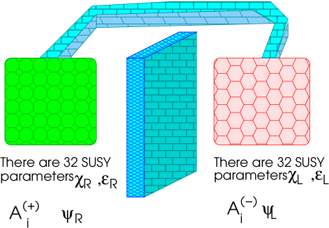
Figure 10: The two-fold SUSY structures of this cubic matrix model. These two worlds are not independent of each other.

However, the relations (4.95) and (4.96) indicate that these two-fold SUSY structures are not independent of each other, but are related with the fields $A^{(\pm)}_{i}$. This is not a beautiful structure, and the physical interpretation of this mixing is not clear yet.

We have seen the SUSY transformation of this cubic matrix model, and this cubic model possesses ${\cal N}=2$ supersymmetry. And analyzing this ${\cal N}=2$ SUSY more deeply, we have clarified the way this cubic model embeds the symmetry of IKKT model : there are two-fold symmetries of 32 fermionic fields, each of which have shown agreement with the SUSY of IKKT model. The investigation of supersymmetry is a powerful tool to analyze the structure of the model.

4.4 The Induction of IKKT model

We have seen the correspondence of this cubic matrix model with IKKT model in terms of the SUSY transformation, and we have shown that this cubic matrix model embeds two supersymmetries of IKKT model, by dividing the chirality of the fermionic parameters. Then here comes a next question :

How can we induce IKKT model from this cubic model?

In this section, we consider the answer to this question, however this is a difficult problem, and we give just a hand-waving argument to this issue.

We have seen the explicit form of the action of this cubic matrix model (4.52) and (4.53). As we have seen in Sec. 3, IKKT model can be interpreted as non-commutative Yang-Mills theory if this theory is expanded around a certain classical solution to the equation of motion [11]. Likewise, the starting point to analyze the behavior is to expand the theory around a classical solution.

This cubic model possesses no time or space derivative from the beginning, as is true of IKKT model. The classical equations of motion should be given by Euler-Lagrange equation of the action (4.52) and (4.53)

$$\partial_{\mu}\frac{\partial I}{\partial(\partial_{\mu}X)}-\frac{\partial I}{\partial X}=0,$$ (4.99)

where $X$ is an arbitrary field of this theory. Since we are interested in the classical solution, we do not consider the fermionic fields in the classical equations of motion. These equations of motion are explicitly given by

$$\frac{\partial I}{\partial W} = -96[A^{(+)}_{i_{1}},A^{(-)i_{1}}]+\frac{4}{5}[I^{(+)}_{i_{1}\cdots i_{5}},I^{(-)i_{1}\cdots i_{5}}]=0,$$ (4.100)

$$\frac{\partial I}{\partial A^{(+)}_{i_{1}}} = -96[A^{(-)}_{i_{2}},C^{i_{1}i_{2}}]+96[W,A^{(-)i_{1}}]+4[H_{i_{2}\cdots i_{5}},I^{(-)i_{1}\cdots i_{5}}]=0,$$

$$\frac{\partial I}{\partial A^{(-)}_{i_{1}}} = -96[A^{(+)}_{i_{2}},C^{i_{1}i_{2}}]-96[W,A^{(+)i_{1}}]-4[H_{i_{2}\cdots i_{5}},I^{(+)i_{1}\cdots i_{5}}]=0,$$ (4.101)

$$\frac{\partial I}{\partial C_{i_{1}i_{2}}} = -96[A^{(+)[i_{1}},A^{(-)i_{2}]}]-8[{I^{(+)[i_{1}}}_{i_{3}\cdots i_{6}},I^{(-)i_{2}]\cdots i_{6}}]+96[{C^{[i_{1}}}_{\rho},C^{i_{2}]\rho}]$$ (4.102)

$$- 16[{H^{[i_{1}}}_{i_{3}\cdots i_{5}},H^{i_{2}]\cdots i_{5}}]=0,$$

$$\frac{\partial I}{\partial H_{i_{1}\cdots i_{4}}} = -4[A^{(+)}_{i_{5}},I^{(-)i_{1}\cdots i_{5}}]+4[A^{(-)}_{i_{5}},I^{(+)i_{1}\cdots i_{5}}]+\frac{8}{3}[{I^{(+)[i_{1}i_{2}}}_{i_{5}i_{6}i_{7}},I^{(-)i_{3}i_{4}]i_{5}i_{6}i_{7}}]$$ (4.103)

$$- \frac{8}{3}[{I^{(-)[i_{1}i_{2}}}_{i_{5}i_{6}i_{7}},I^{(+)i_{3}i_{4}]i_{5}i_{6}i_{7}}]-32[{C_{\rho}}^{[i_{1}},H^{\rho i_{2}i_{3}i_{4}]}]+\frac{1}{54}[{I^{\rho\sigma}}_{i_{5}i_{6}i_{7}},I_{\rho\sigma i_{8}i_{9}i_{10}}]\epsilon^{i_{1}\cdots i_{10}\sharp}$$

$$+ \frac{1}{27}[{H^{\rho}}_{i_{5}i_{6}i_{7}},H_{\rho i_{8}i_{9}i_{10}}]\epsilon^{i_{1}\cdots i_{10}\sharp}+\frac{2}{27}[{H^{i_{1}}}_{i_{5}i_{6}i_{7}},H_{i_{8}\cdots i_{11}}]\epsilon^{i_{2}\cdots i_{11}\sharp}=0,$$

$$\frac{\partial I}{\partial I^{(+)}_{i_{1}\cdots i_{5}}} = \frac{-4}{5}[W,I^{(-)i_{1}\cdots i_{5}}]-4[A^{(-)[i_{1}},H^{i_{2}\cdots i_{5}]}]-8[C^{k[i_{1}},{{I^{(-)}}_{k}}^{i_{2}\cdots i_{5}]}]-\frac{16}{3}[{H_{kl}}^{[i_{1}i_{2}},I^{(-)kli_{3}i_{4}i_{5}]}]=0,$$

$$\frac{\partial I}{\partial I^{(-)}_{i_{1}\cdots i_{5}}} = \frac{4}{5}[W,I^{(+)i_{1}\cdots i_{5}}]+4[A^{(+)[i_{1}},H^{i_{2}\cdots i_{5}]}]-8[C^{k[i_{1}},{{I^{(+)}}_{k}}^{i_{2}\cdots i_{5}]}+\frac{16}{3}[{H_{kl}}^{[i_{1}i_{2}},I^{(+)kli_{3}i_{4}i_{5}]}]=0.$$ (4.104)

Now, we consider the classical solution of the above equations of motion. It is almost impossible to solve the above equations of motions exactly, but we can find a classical solution which possesses a physical consequence. As we have seen in the case of IKKT model, the canonical pairs play an essential role in introducing kinetic terms of the theory:

$$A^{(+)}_{0}=p_{1},A^{(+)}_{1}=q_{1},\cdots A^{(+)}_{2d-2}=p_{d},A^{(+)}_{2d-1}=q_{d},\textrm{ (all the other fields)}=0,$$ (4.105)

where $p_{k},q_{l}$ are $d$ independent pairs of canonical pairs satisfying $[q_{k},p_{l}]=i\delta_{kl}$. $2d$ is a number of the dimension of the spacetime produced by this classical solution, and we now focus on the case in which $2d=10$. If we expand the theory around this classical solution, we can introduce the spacetime derivative in the same fashion as in IKKT model [11]. We separate the field $A^{(+)}_{i}$ between the classical solution and the fluctuation:

$$A^{(+)}_{i}={\hat{p}}_{i}+a^{(+)}_{i},$$ (4.106)

where ${\hat{p}}_{i}$ denotes the above classical solution. We can then introduce a spacetime derivative by mapping the commutators with the $A^{(+)}_{i}$ fields with the covariant derivative, where $X$ is an arbitrary field,

$$[A^{(+)}_{i},X]=-i\partial_{i}X+[a^{(+)}_{i},X].$$ (4.107)

Applying this mapping rule to the action (4.52) and (4.53), we can introduce a kinetic term in this action, and thus we obtain the following action:

$$I_{b} = \frac{1}{g^{2}}Tr_{N\times N}(-96(\partial_{i_{1}}A^{(-)}_{i_{2}})C^{i_{1}i_{2}}+96(\partial_{i}W)A^{(-)i}+4(\partial_{i_{1}}H_{i_{2}\cdots i_{5}})I^{(-)i_{1}\cdots i_{5}})$$

$$+ \frac{i}{g^{2}}Tr_{N\times N}(-96[a^{(+)}_{i_{1}},A^{(-)}_{i_{2}}]C^{i_{1}i_{2}}-96W[a^{(+)i},A^{(-)}_{i}]+\frac{4}{5}W[I^{(+)}_{i_{1}\cdots i_{5}},I^{(-)i_{1}\cdots i_{5}}]$$

$$+ 4([a^{(+)}_{i_{1}},H_{i_{2}\cdots i_{5}}]I^{(-)i_{1}\cdots i_{5}}-[A^{(-)}_{i_{1}},H_{i_{2}\cdots i_{5}}]I^{(+)i_{1}\cdots i_{5}})-8C_{i_{1}i_{2}}[{I^{(+)i_{1}}}_{i_{3}\cdots i_{6}},I^{(-)i_{2}\cdots i_{6}}]$$

$$+ \frac{8}{3}{H^{kl}}_{i_{1}i_{2}}([{I^{(+)}}_{kli_{3}i_{4}i_{5}},I^{(-)i_{1}\cdots i_{5}}]-[{I^{(-)}}_{kli_{3}i_{4}i_{5}},I^{(+)i_{1}\cdots i_{5}}])$$

$$+ 32[{C^{i_{1}}}_{i_{2}},C_{i_{1}i_{3}}]C^{i_{2}i_{3}}-16C_{i_{1}i_{2}}[{H^{i_{1}}}_{i_{3}i_{4}i_{5}},H^{i_{2}\cdots i_{5}}]+\frac{1}{27}H_{i_{1}\cdots i_{4}}[{H^{k}}_{i_{5}\cdots i_{7}},H_{ki_{8}i_{9}i_{10}}]\epsilon^{i_{1}\cdots i_{10}\sharp}),$$ (4.109)

$$I_{f} = \frac{1}{g^{2}}Tr_{N\times N}(-3i{\bar{\psi}_{L}}\Gamma^{i}\partial_{i}\psi_{L})$$

$$+ \frac{i}{g^{2}}Tr_{N\times N}(-3i(-{\bar{\psi}_{L}}[W,\psi_{R}]+{\bar{\psi}_{R}}[W,\psi_{L}])-3i({\bar{\psi}_{L}}\Gamma^{i}[a^{(+)}_{i},\psi_{L}]+{\bar{\psi}_{R}}\Gamma^{i}[A^{(-)}_{i},\psi_{R}])$$

$$- \frac{3i}{2!}({\bar{\psi}_{L}}\Gamma^{i_{1}i_{2}}[C_{i_{1}i_{2}},\psi_{R}]+{\bar{\psi}_{R}}\Gamma^{i_{1}i_{2}}[C_{i_{1}i_{2}},\psi_{L}])-\frac{3i}{4!}(-{\bar{\psi}_{L}}\Gamma^{i_{1}i_{2}i_{3}i_{4}}[H_{i_{1}i_{2}i_{3}i_{4}},\psi_{R}]+{\bar{\psi}_{R}}\Gamma^{i_{1}i_{2}i_{3}i_{4}}[H_{i_{1}i_{2}i_{3}i_{4}},\psi_{L}])$$

$$- \frac{3i}{5!}(2{\bar{\psi}_{L}}\Gamma^{i_{1}i_{2}i_{3}i_{4}i_{5}}[{I^{(+)}}_{i_{1}i_{2}i_{3}i_{4}i_{5}},\psi_{L}]+2{\bar{\psi}_{R}}\Gamma^{i_{1}i_{2}i_{3}i_{4}i_{5}}[{I^{(-)}}_{i_{1}i_{2}i_{3}i_{4}i_{5}},\psi_{R}])).$$ (4.111)

The cubic action, per se, does not include a quartic term of vector fields in the action. However, we can interpret that the bosonic term is induced by the fermionic term of the IKKT model. The idea that the theory consisting of fermionic fields and a Dirac operator induces Einstein gravity and Yang-Mills theory has long been suggested. The proposal of Connes and Chamseddine is one of these suggestions of induced gravity [3]. Based on these suggestions, we find it a natural idea that the bosonic term of IKKT model is induced from its fermionic term. And we hypothesize that the whole IKKT model should be induced only by the fermionic field.

Our goal is thus to find the fermionic terms in this cubic matrix model to be identified with that of IKKT model. We have seen in the previous section the correspondence between the vector fields and the fermionic fields according to the identification of ${\cal N}=2$ SUSY with that of IKKT model. And the fermionic terms to be identified with that if IKKT model is

$${\bar{\psi}_{R}}\Gamma^{i}A^{(+)}_{i}\psi_{R}\stackrel{{\scriptstyle or}}{{\Leftrightarrow}}{\bar{\psi}_{L}}\Gamma^{i}A^{(-)}_{i}\psi_{L}.$$ (4.112)

If either of these terms exists in the action, this can be identified with the fermionic term of IKKT model. However, the kinetic term of the fermionic fields (4.4), per se, does not include such terms as (4.112), and does not serve to induce IKKT model due to the discrepancy of the correspondence of the vector fields and the chirality of the fermions. In order to remedy this situation, we consider inducing the terms (4.112) by multi-loop effect. The action (4.4) $\sim$ (4.111) just tells us that there is no terms to be identified with IKKT model at a tree level. Since the idea of ’induced IKKT model’ is to construct the bosonic term by one-loop effect of fermionic Lagrangian, the idea of ’induced theory’ is, per se, a notion based on multi-loop effect of the perturbative theory. In this sense, there is no problem if the fermionic term is induced by the multi-loop effect.

In order to consider the multi-loop effect of the cubic theory, we start from considering the Feynman diagram of this theory. The kinetic terms contributes to the propagators, and the cubic terms contributes to the vertices of this theory. These Feynman rules can be read off from the action (4.4) $\sim$ (4.111).

• Propagator : The propagators of this cubic matrix theory stems from the kinetic terms (4.4) and (4.4).

  

  Figure 11: Propagators of this cubic matrix theory.

  Apparently, the action (4.4) $\sim$ (4.111) seems to include the propagators $\langle WA^{(-)i}\rangle$, $\langle A^{(-)}_{i}C^{ij}\rangle$, $\langle H_{jklm}I^{(-)ijklm}\rangle$ and $\langle\psi_{L}\psi_{L}\rangle$. However, a careful investigation of this theory reveals that the propagator $\langle A^{(-)}_{i}C^{ij}\rangle$ is prohibited from existing, while the other propagators $\langle WA^{(-)}_{i}\rangle$, $\langle H_{jklm}I^{(-)ijklm}\rangle$ and $\langle\psi_{L}\psi_{L}\rangle$ do exist in this theory. We leave the discussion of the existence of these propagators to Appendix. B.3.

• Vertex: This is also read off from the action of this theory.

  

  Figure 12: Vertices of this cubic matrix theory.

  Of course, the vertices for the fields of higher rank (such as $H_{i_{1}\cdots i_{4}}$ and $I^{(\pm)}_{i_{1}\cdots i_{5}}$) exist, however we omit drawing their Feynman diagrams because these diagrams do not contribute to our discussion of inducing IKKT model.

Our goal is to build a fermion vertex (4.112) by means of the multi-loop effect. In order to build such a term, the above Feynman diagrams do not suffice. Especially we are lacking the propagators of the fields. It is thus necessary to build an induced propagators by means of the multi-loop effect of the existing Feynman rule. These induced propagators are constructed by the following loop effect.

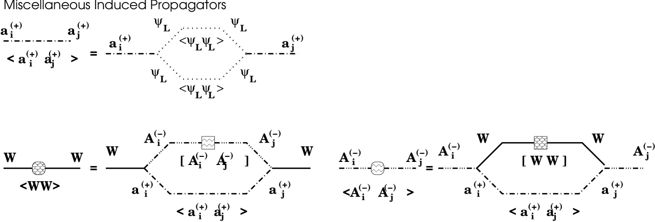
Figure 13: The induced propagators of the bosonic fields

• $\langle a^{(+)}_{i}a^{(+)}_{j}\rangle$ : It is easy to construct this induced propagator. All we have to do is to connect the fermions using the existing fermion propagators $\langle\psi_{L}\psi_{L}\rangle$.

• $\langle WW\rangle$ and $\langle A^{(-)}_{i}A^{(-)}_{j}\rangle$ : The construction of these propagators is a difficult problem. Unfortunately, it is impossible to construct these propagators perturbatively, and we disprove their existence in Appendix. B.4. However, this is not the end of the story. Even if we fail to induce these propagators perturbatively, we have a choice to induce these propagators by means of the nonperturbative effect. These propagators may be induced by the following recursive structure.

  

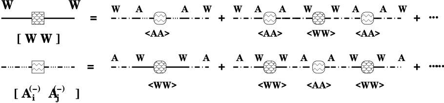
  Figure 14: The induced propagators of the bosonic fields

  This structure is reminiscent of the self-consistency condition of Nambu-Jona-Lasino model. And when we consider the nonperturbative effect, there is no particular conservation law which prohibits the existence of the propagators $\langle WW\rangle$ or $\langle A^{(-)}_{i}A^{(-)}_{j}\rangle$ . Throughout our discussion, we assume the existence of these propagators.

Now we are ready to construct the induced propagators of this cubic model. In constructing the vertices of the fermionic terms (4.112). The answer is now easy, and the IKKT-like vertex is constructed by the following procedure.

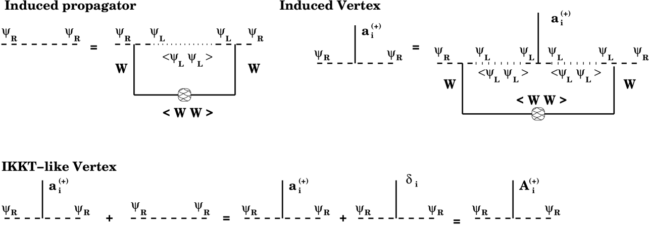
Figure 15: The induced IKKT-like vertex ${\bar{\psi}}\Gamma^{i}A^{(+)}_{i}\psi$

• To construct the induced vertex corresponding to (4.112), we must first construct two objects. One is the propagator $\langle\psi_{R}\psi_{R}\rangle$. This is easily constructed once we admit the existence of the propagator $\langle WW\rangle$.

• Another object is the vertex ${\bar{\psi}_{R}}\Gamma^{i}a^{(+)}_{i}\psi_{R}$. It is also easy to construct this vertex utilizing the induced propagator $\langle WW\rangle$.

• These two objects serve to induce our desired term ${\bar{\psi}_{R}}\Gamma^{i}A^{(+)}_{i}\psi_{R}$. Note that this induced propagator indicates that the kinetic term ${\bar{\psi}_{R}}\Gamma^{i}\partial_{i}\psi_{R}$. This is diagrammatically regarded as the vertex of $\psi_{R}$, $\psi_{R}$ and $\partial_{i}\sim{\hat{p}}_{i}$, where ${\hat{p}}_{i}$ is the classical solution (4.105), around which we have expanded the theory. Therefore, the sum of these two objects is regarded as

  $$\langle\psi_{R}\psi_{R}\rangle+{\bar{\psi}_{R}}\Gamma^{i}a^{(+)}_{i}\psi_{R}=-i{\bar{\psi}_{R}}\partial_{i}\psi_{R}+{\bar{\psi}_{R}}\Gamma^{i}a^{(+)}_{i}\psi_{R}={\bar{\psi}_{R}}\Gamma^{i}A^{(+)}_{i}\psi_{R}.$$ (4.113)

Now, we have completed constructing the fermionic term to be identified with that of IKKT model, considering the correspondence of ${\cal N}=2$ SUSY transformation:

$$I\sim{\bar{\psi}_{R}}\Gamma^{i}A^{(+)}_{i}\psi_{R}.$$ (4.114)

Now, here comes two objections of the prosecutor to our argument.

1. One objection is that we have yet to succeed in decoupling the fermions. Even though we have constructed the fermionic term ${\bar{\psi}_{R}}\Gamma^{i}A^{(+)}_{i}\psi_{R}$, the term ${\bar{\psi}_{L}}\Gamma^{i}A^{(+)}_{i}\psi_{L}$ is still mixed in this action, and we have no system to decouple the ’impurity’ ${\bar{\psi}_{L}}\Gamma^{i}A^{(+)}_{i}\psi_{L}$. Then, it may be artificial to extract the desired term ${\bar{\psi}_{R}}\Gamma^{i}A^{(+)}_{i}\psi_{R}$ by hand, and it cannot be said that the fermionic term of IKKT model is naturally induced.

2. The other objection is that we have assumed the existence of the propagator $\langle WW\rangle$ and $\langle A^{(-)}_{i}A^{(-)}_{j}\rangle$. The analogue of Nambu-Jona-Lasino model can only assert that, if such propagators exist, these are due to the nonperturbative effect. Like Nambu-Jona-Lasino model, we are required to investigate the existence of the solution of self-consistency condition. We have not succeeded in verifying the existence of these propagators.

These are fatal objections to our discussion, however the pleader refutes these objections as follows.

1. For the first problem, we have a viewpoint that the fermion $\psi_{L}$ is integrated out in constructing the vertex operator ${\bar{\psi}_{R}}\Gamma^{i}A^{(+)}_{i}\psi_{R}$. Since we have performed a loop integration with respect to the fermionic propagator $\langle\psi_{L}\psi_{L}\rangle$, it is a natural interpretation that the $\psi_{L}$ has been integrated out and no longer exists in the effective theory. We reckon this integration as the system to ostracize the impurity ${\bar{\psi}_{L}}\Gamma^{i}A^{(+)}_{i}\psi_{L}$ from the theory.

2. The latter is a tough objection, and we have yet to find a definite answer. However, there is no physical conservation law to prohibit the existence of these propagators, and we consider the existence of these propagators to be a decent hypothesis.

The action with only the fermionic term of the theory is known to induce the bosonic part of IKKT model. The bosonic part stems from the one-loop effect of this fermionic vertex, as shown in Fig. 16. These induced terms $(A^{(\pm)}_{i})^{2}$ are conjectured to emerge as a commutator $[A^{(\pm)}_{i},A^{(\pm)}_{j}]$. Therefore, we can speculate that this cubic matrix model may induce IKKT model by the multi-loop effect:

$$I_{IKKT}=-\frac{1}{g^{2}_{IKKT}}(\frac{1}{4}[A_{IKKTi},A_{IKKTj}][A_{IKKT}^{i},A_{IKKT}^{j}]+\frac{1}{2}{\bar{\psi}}_{IKKT}\Gamma_{i}[A_{IKKT}^{i},\psi_{IKKT}].$$ (4.115)

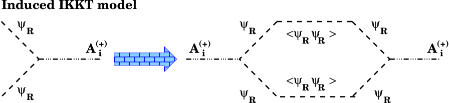
Figure 16: Induced IKKT model from the fermionic term. The bosonic term will be induced by the one-loop effect.

Although we have developed just a hand-waving argument, it may at least indicate a sign that this $osp(1|32,R)$ cubic model has a scenario to induce IKKT model, with the induced terms agreeing with the correspondence of the identification of ${\cal N}=2$ SUSY.

4.5 Summary

Let us conclude this section by summarizing the discussion concerning the $osp(1|32,R)$ cubic matrix model.

• L. Smolin suggested a new type of cubic matrix theory:

  $$I = \frac{i}{g^{2}}Tr_{N\times N}\sum_{Q,R=1}^{33}((\sum_{p=1}^{32}{M_{p}}^{Q}[{M_{Q}}^{R},{M_{R}}^{p}])-{M_{33}}^{Q}[{M_{Q}}^{R},{M_{R}}^{33}])$$

  $$= \frac{i}{g^{2}}\sum_{a,b,c=1}^{N^{2}}Str(M^{a}M^{b}M^{c})Tr(T^{a}[T^{b},T^{c}]).$$

  The biggest novelty of this cubic matrix model lies in the fact that both bosons and fermions are embedded in one multiplet of super Lie algebra $osp(1|32,R)$.

• This cubic model possesses two-fold ${\cal N}=2$ SUSY structures, each for 32 fermionic SUSY parameters. Each of these two-fold SUSY structures is identified with the ${\cal N}=2$ SUSY of IKKT model. The correspondence of the fields of the cubic model and those of IKKT model is as follows.
  

  	bosons $A_{i}$ (IKKT)	fermions $\psi$(IKKT)
  SUSY I	$A^{(+)}_{i}$	$\psi_{R}=\frac{1-\Gamma^{\sharp}}{2}\psi$
  SUSY II	$A^{(-)}_{i}$	$\psi_{L}=\frac{1+\Gamma^{\sharp}}{2}\psi$

  However, these two-fold SUSY’s are not independent of each other, but are connected by the fields $A^{(\pm)}_{i}$, the very fields to be identified with those of IKKT model.

• We speculate by a hand-waving argument that this cubic model induces IKKT model by a multi-loop effect of the fermionic term. And we constructed the fermionic terms with the correspondence with the vector fields imposed by the identification of ${\cal N}=2$ SUSY. This can be regarded as the induced IKKT model, with the bosonic part induced by the fermionic part.

Our discussion in this section solidifies the conjecture that Smolin’s proposal may naturally include IKKT model, as is predictable from the symmetry of $osp(1|32,R)$ super Lie algebra. However, our scenario to derive IKKT model from Smolin’s proposal is hand-waving, and it is an issue of interest and importance to pursue a more solid scenario. If we succeed in proving the embedding of IKKT model in a more natural way, we will be more convinced that Smolin’s proposal truly exceeds IKKT model.

5 $gl(1|32,R)\otimes gl(N,R)$ Gauged Cubic Matrix Model

We have seen a new proposal for the constructive definition of superstring theory in the previous chapter, and we have considered the cubic matrix model with the multiplet belonging to $osp(1|32,R)$ super Lie algebra. However, it is an interesting problem to consider the extended version of this model. The action we investigate here is named ’gauged’ action in terms of Smolin’s proposal [13] [17]. The action is described by the following formula:

$$I=\frac{1}{g^{2}}Tr_{N\times N}\sum_{Q,R=1}^{33}((\sum_{p=1}^{32}{M_{p}}^{Q}{M_{Q}}^{R}{M_{R}}^{p})-{M_{33}}^{Q}{M_{Q}}^{R}{M_{R}}^{33})=\frac{1}{g^{2}}Tr_{N\times N}(Str_{33\times 33}M^{3}).$$ (5.1)

This action is characterized by the fact that we have promoted the tensor product of the two gauge group from that of Lie groups ($\times$) to that of Lie algebra ($\otimes$). The difference of these two notions has been treated in Appendix. A.5. This action is in this sense named ’gauged action’ Although this action is deprived of the translation symmetry, the symmetry of this action possesses far larger gauge symmetry because the direct product is promoted to the tensor product of two matrices.

Originally L. Smolin proposed this new version as a complexification of $osp(1|32,R)$ matrix model, and the super Lie algebra is taken to be $u(1|16,16)$. The complexification of $osp(1|32,R)$ matrix model has enriched the symmetry of the theory, and Smolin conjectures that this gauged theory may include loop quantum gravity [17].

We investigate a real version of Smolin’s proposal, rather than the original $u(1|16,16)$ multiplets. The matrix model we pursue can be obtained by the ’analytic continuation’ of Smolin’s proposal in two respects.

• We adopt $gl(1|32,R)$ super Lie algebra as a symmetry of this action. This is a super Lie algebra composed of real supermatrix.

• We take the gauge symmetry of large $N$ matrices as a real Lie algebra $(N)$, rather than $su(N)$.

Throughout this chapter, we focus on the $gl(1|32,R)\otimes gl(N,R)$ gauge symmetry. In this section, we sometimes refer to the relationship between our argument and the features of $u(1|16,16)$ gauge symmetry, which is a cousin of our $gl(1|32,R)\otimes gl(N,R)$ gauge group.

5.1 Definition of $gl(1|32,R)$ Super Lie Algebra

This section is devoted to introducing the super Lie algebra $gl(1|32,R)$, noting the difference from the cousin $u(1|16,16)$ super Lie algebra, which is introduced as a complexification of $osp(1|32,R)$ super Lie algebra. Here we make a bit of excursion of the complex $u(1|16,16)$ super Lie algebra, and then we define $gl(1|32,R)$ super Lie algebra and compare these two super Lie algebras.

5.1.1 Excursion of $u(1|16,16)$ Super Lie Algebra

The very definition of this super Lie algebra is that

$$\textrm{ If }M\in u(1|16,16),\textrm{ then }M^{\dagger}G+GM=0\textrm{ for }G=\left(\begin{array}[]{cc}\Gamma^{0}&0\\ 0&i\end{array}\right).$$ (5.4)

That this is a complexification of $osp(1|32,R)$ can be seen from the following aspect. Unlike the $osp(1|32,R)$ super Lie algebra, we do not restrict $M$ to be a real supermatrix, where the reality of the supermatrix is defined as $M=M^{\ast}=({{}^{T}M})^{\dagger}$. Therefore, we must replace the transpose by the hermitian conjugate. Note that in the real version the complex conjugate is equivalent to the transpose according to the property in Appendix. A.3.

We can confirm that the super Lie algebra $u(1|16,16)$ actually closes in totally the same fashion as in $osp(1|32,R)$. The legitimacy of the metric also stems from the same logic as in $osp(1|32,R)$. We specify the element of $u(1|16,16)$ group according to the above definition. The result is that

$$\textrm{ If }M\in u(1|16,16),\textrm{ then }M=\left(\begin{array}[]{cc}m&\psi\\ i{\bar{\psi}}&v\end{array}\right).$$ (5.7)

• $v$ is restricted to be a pure imaginary number.

• $u_{\mu_{1}}$ ,$u_{\mu_{1}\mu_{2}}$ and $u_{\mu_{1}\cdots\mu_{5}}$ are real numbers, while $u$, $u_{\mu_{1}\mu_{2}\mu_{3}}$ and $u_{\mu_{1}\cdots\mu_{4}}$ are pure imaginary numbers.

• Here ${\bar{\psi}}$ denotes $\psi^{\dagger}\Gamma^{0}$.

(Proof) This result is derived from the very definition of the super Lie algebra $u(1|16,16)$. The complex conjugate of supermatrices is defined in Appendix. A.3:

$$M^{\dagger}G+GM=\left(\begin{array}[]{cc}m^{\dagger}&\phi\\ \psi^{\dagger}&v^{\dagger}\end{array}\right)\left(\begin{array}[]{cc}\Gamma^{0}&0\\ 0&i\end{array}\right)+\left(\begin{array}[]{cc}\Gamma^{0}&0\\ 0&i\end{array}\right)\left(\begin{array}[]{cc}m&\psi\\ \phi^{\dagger}&v\end{array}\right)=\left(\begin{array}[]{cc}m^{\dagger}\Gamma^{0}+\Gamma^{0}m&i\phi+\Gamma^{0}\psi\\ \psi^{\dagger}\Gamma^{0}+i\phi^{\dagger}&i(v+v^{\dagger})\end{array}\right)=0.$$ (5.18)

• It is a trivial matter to understand that $v$ is a pure imaginary number from $v+v^{\dagger}=0$.

• We first investigate the constraint of the bosonic matrix $m$. These are decomposed, as we have done in $osp(1|32,R)$ matrix model, in terms of the basis of gamma matrices:

  $$m = u{\bf 1}+u_{\mu_{1}}\Gamma^{\mu_{1}}+\frac{1}{2!}u_{\mu_{1}\mu_{2}}\Gamma^{\mu_{1}\mu_{2}}+\frac{1}{3!}u_{\mu_{1}\mu_{2}\mu_{3}}\Gamma^{\mu_{1}\mu_{2}\mu_{3}}+\frac{1}{4!}u_{\mu_{1}\cdots\mu_{4}}\Gamma^{\mu_{1}\cdots\mu_{4}}+\frac{1}{5!}u_{\mu_{1}\cdots\mu_{5}}\Gamma^{\mu_{1}\cdots\mu_{5}}.$$

  We utilize the relationship of the gamma matrices ${{}^{T}\Gamma^{\mu_{1}\cdots\mu_{k}}}\Gamma^{0}=\pm\Gamma^{0}\Gamma^{\mu_{1}\cdots\mu_{k}}$ with the sign $+$ for $k=1,2,5$ and the sign $-$ for $k=0,3,4$. The reveals that the coefficients must satisfy the following results.

  • $(u_{\mu_{1}\cdots\mu_{k}})^{\ast}=u_{\mu_{1}\cdots\mu_{k}}$ for $k=1,2,5$. These are thus restricted to be real numbers.

  • $(u_{\mu_{1}\cdots\mu_{k}})^{\ast}=-u_{\mu_{1}\cdots\mu_{k}}$ for $k=0,3,4$ These are thus restricted to be pure imaginary numbers.

• We investigate the relationship between two fermions $\psi$ and $\phi^{\dagger}$ utilizing the result $i\phi+\Gamma^{0}\psi=0$:

  $$\phi^{\dagger}=(i\Gamma^{0}\psi)^{\dagger}=(-i)\psi^{\dagger}({{}^{T}\Gamma^{0}})=(-i)\psi^{\dagger}(-\Gamma^{0})=i{\bar{\psi}}.$$ (5.19)

  We can verify that this is consistent with the condition ${\psi}^{\dagger}\Gamma^{0}+i{\phi}^{\dagger}=0$.

We are thus finished with the determination of the elements of $U(1|16,16)$ super Lie algebra. (Q.E.D.)

The important property of $u(1|16,16)$ super Lie algebra is that these can be uniquely decomposed into the direct sum of two different representations of $osp(1|32,R)$. We introduce two different representations of $osp(1|32,R)$ super Lie algebra

$$\clubsuit {\cal H}\stackrel{{\scriptstyle def}}{{=}}\{M=\left(\begin{array}[]{cc}m_{h}&\psi_{h}\\ i{\bar{\psi}_{h}}&0\end{array}\right)|m_{h}=u_{\mu_{1}}\Gamma^{\mu_{1}}+\frac{1}{2!}u_{\mu_{1}\mu_{2}}\Gamma^{\mu_{1}\mu_{2}}+\frac{1}{5!}u_{\mu_{1}\cdots\mu_{5}}\Gamma^{\mu_{1}\cdots\mu_{5}},$$

$$\hskip 128.0374ptu_{\mu_{1}},u_{\mu_{1}\mu_{2}},u_{\mu_{1}\cdots\mu_{5}},\psi_{h}\in{\cal R}\},$$

$$\clubsuit {\cal A}^{\prime}\stackrel{{\scriptstyle def}}{{=}}\{M=\left(\begin{array}[]{cc}m_{a}&i\psi_{a}\\ {\bar{\psi}_{a}}&iv\end{array}\right)|m_{a}=u+\frac{1}{3!}u_{\mu_{1}\mu_{2}\mu_{3}}\Gamma^{\mu_{1}\mu_{2}\mu_{3}}+\frac{1}{4!}u_{\mu_{1}\cdots\mu_{4}}\Gamma^{\mu_{1}\cdots\mu_{4}},$$

$$\hskip 128.0374ptu,u_{\mu_{1}\mu_{2}\mu_{3}},u_{\mu_{1}\cdots\mu_{4}},i\psi_{a},iv\in(\textrm{pure imaginary})\}.$$

And let $H$ and $A^{\prime}$ be the element of ${\cal H}$ and ${\cal A}^{\prime}$ respectively. Because these are real (pure imaginary), these elements respectively satisfy $H^{\dagger}={{}^{T}H^{\prime}}$ and $A^{\prime\dagger}=-{{}^{T}A^{\prime}}$. Therefore, these elements satisfy the following property

$${{}^{T}H}G+GH=0,\textrm{ for }H\in{\cal H},\hskip 8.53581pt{{}^{T}A}^{\prime}G-GA^{\prime}=0,\textrm{ for }A^{\prime}\in{\cal A}^{\prime}.$$ (5.26)

The set ${\cal H}$ is, by definition, $osp(1|32,R)$ super Lie algebra itself. We investigate an important property of the subset of these two subalgebras. The commutation and anti-commutation relations are properties of grave importance in getting acquainted with the Algebras of these groups.

$$(1)[H_{1},H_{2}]\in{\cal H},\hskip 8.53581pt(2)[H,A^{\prime}]\in{\cal A}^{\prime},\hskip 8.53581pt(3)[A^{\prime}_{1},A^{\prime}_{2}]\in{\cal H},$$

$$(4)\{H_{1},H_{2}\}\in{\cal A}^{\prime},\hskip 8.53581pt(5)\{H,A^{\prime}\}\in{\cal H},\hskip 8.53581pt(6)\{A^{\prime}_{1},A^{\prime}_{2}\}\in{\cal A}^{\prime}.$$ (5.27)

where $H,H_{1},H_{2}\in{\cal H}$ and $A^{\prime},A^{\prime}_{1},A^{\prime}_{2}\in{\cal A^{\prime}}$.
(Proof) These properties can be verified by noting the properties (5.26).

1. ${{}^{T}[H_{1},H_{2}]}G={{}^{T}H_{2}}{{}^{T}H_{1}}G-{{}^{T}H_{1}}{{}^{T}H_{2}}G={{}^{T}H_{2}}(-GH_{1})-{{}^{T}H_{1}}(-GH_{2})=GH_{2}H_{1}-GH_{1}H_{2}=-G[H_{1},H_{2}]$,

2. ${{}^{T}[H,A^{\prime}]}G={{}^{T}A^{\prime}}{{}^{T}H}G-{{}^{T}H}{{}^{T}A^{\prime}}G={{}^{T}A^{\prime}}(-GH)-{{}^{T}H}(GA^{\prime})=-GA^{\prime}H+GHA^{\prime}=G[H,A^{\prime}]$,

3. ${{}^{T}[A^{\prime}_{1},A^{\prime}_{2}]}G={{}^{T}A^{\prime}_{2}}{{}^{T}A^{\prime}_{1}}G-{{}^{T}A^{\prime}_{1}}{{}^{T}A^{\prime}_{2}}G={{}^{T}A^{\prime}_{2}}(GA^{\prime}_{1})-{{}^{T}A^{\prime}_{1}}(GA^{\prime}_{2})=GA^{\prime}_{2}A^{\prime}_{1}-GA^{\prime}_{1}A^{\prime}_{2}=-G[A^{\prime}_{1},A^{\prime}_{2}]$,

4. ${{}^{T}\{H_{1},H_{2}\}}G={{}^{T}H_{2}}{{}^{T}H_{1}}G+{{}^{T}H_{1}}{{}^{T}H_{2}}G={{}^{T}H_{2}}(-GH_{1})+{{}^{T}H_{1}}(-GH_{2})=GH_{2}H_{1}+GH_{1}H_{2}=G\{H_{1},H_{2}\}$,

5. ${{}^{T}\{H_{1},A^{\prime}_{1}\}}G={{}^{T}A^{\prime}_{1}}{{}^{T}H_{1}}G+{{}^{T}H_{1}}{{}^{T}A^{\prime}_{1}}G={{}^{T}A^{\prime}_{1}}(-GH_{1})+{{}^{T}H_{1}}(GA^{\prime}_{1})=-GA^{\prime}_{1}H_{1}-GH_{1}A^{\prime}_{1}=-G\{H_{1},A^{\prime}_{1}\}$,

6. ${{}^{T}\{A^{\prime}_{1},A^{\prime}_{2}\}}G={{}^{T}A^{\prime}_{2}}{{}^{T}A^{\prime}_{1}}G+{{}^{T}A^{\prime}_{1}}{{}^{T}A^{\prime}_{2}}G={{}^{T}A^{\prime}_{2}}GA^{\prime}_{1}+{{}^{T}A^{\prime}_{1}}GA^{\prime}_{2}=GA^{\prime}_{2}A^{\prime}_{1}+GA^{\prime}_{1}A^{\prime}_{2}=G\{A^{\prime}_{1},A^{\prime}_{2}\}$.

This completes the proof of the above properties. (Q.E.D.)

Utilizing these relations, we can discern that ${\cal A}^{\prime}$, as well as ${\cal H}^{\prime}$ is the representations of $osp(1|32,R)$ and also that the algebra ${\cal A}^{\prime}$ is a representation of $osp(1|32,R)$ super Lie algebra by the commutation relation $(2)[H,A^{\prime}]\in{\cal A}^{\prime}$ for $H\in{\cal H}$ and $A^{\prime}\in{\cal A}^{\prime}$. This commutation relation states that $A^{\prime}$ remain in the super Lie algebra ${\cal A}^{\prime}$ after the infinitesimal translation by the elements $H\in{\cal H}$. In this sense, we can understand that ${\cal A}^{\prime}$ is another representation of $osp(1|32,R)$.

The introduction of these two representations of $osp(1|32,R)$ teaches us the relationship of $osp(1|32,R)$ and $u(1|16,16)$ super Lie algebras. ${\cal H}(=osp(1|32,R))$ is a real part of $u(1|16,16)$ Lie algebra, while ${\cal A}^{\prime}$ is its imaginary part. It is clear that the elements of $u(1|16,16)$ can be uniquely decomposed into the direct sum of ${\cal H}$ and ${\cal A}^{\prime}$.

$$u(1|16,16)\equiv{\cal H}\oplus{\cal A}^{\prime},$$ (5.28)

where $\oplus$ denotes the direct sum of two sets.

5.1.2 Definition of $gl(1|32,R)$ Super Lie Algebra

The definition of $gl(1|32,R)$ super Lie algebra is, per se, simple:

$$\clubsuit \textrm{If }M\in gl(1|32,R),\hskip 8.53581pt\textrm{ then }M=\left(\begin{array}[]{cc}m&\psi\\ i{\bar{\phi}}&v\end{array}\right).$$ (5.31)

• $m$ is an element of the Lie algebra $gl(32,R)$, id est, $m$ is allowed to be an arbitrary $32\times 32$ bosonic matrix. Decomposing this by the gamma matrices, this can be expressed by

  $$m=u{\bf 1}+u_{\mu_{1}}\Gamma^{\mu_{1}}+\frac{1}{2!}u_{\mu_{1}\mu_{2}}\Gamma^{\mu_{1}\mu_{2}}+\frac{1}{3!}u_{\mu_{1}\mu_{2}\mu_{3}}\Gamma^{\mu_{1}\mu_{2}\mu_{3}}+\frac{1}{4!}u_{\mu_{1}\cdots\mu_{4}}\Gamma^{\mu_{1}\cdots\mu_{4}}+\frac{1}{5!}u_{\mu_{1}\cdots\mu_{5}}\Gamma^{\mu_{1}\cdots\mu_{5}},$$ (5.32)

  where the coefficients $u_{\mu_{1}\cdots}$ are all real numbers.

• $\psi$ and $\phi$ are independent fermionic vectors. Each of them possesses 32 components, and the components are fermionic real number.

• $v$ is also a real number.

The definition of $gl(1|32,R)$ states nothing. This definition just states that an arbitrary real $33\times 33$ supermatrix is an eligible member of the super Lie algebra $gl(1|32,R)$. Although this definition does not give any restriction to the elements, the correspondence with the complex group $u(1|16,16)$ is an interesting aspect of $gl(1|32,R)$ super Lie algebra. Since $\psi$ and $\phi$ are independent fermionic vectors, these can be rewritten as

$$\psi=\psi_{1}+\psi_{2},\hskip 5.69054pt\phi=\psi_{1}-\psi_{2}.$$ (5.33)

And the bosonic $32\times 32$ matrices are separated by $m=m_{1}+m_{2}$, where

$$m_{1}=u_{\mu_{1}}\Gamma^{\mu_{1}}+\frac{1}{2!}u_{\mu_{1}\mu_{2}}\Gamma^{\mu_{1}\mu_{2}}+\frac{1}{5!}u_{\mu_{1}\cdots\mu_{5}}\Gamma^{\mu_{1}\cdots\mu_{5}},\textrm{ where }u_{\mu_{1}},u_{\mu_{1}\mu_{2}},u_{\mu_{1}\cdots\mu_{5}}\textrm{ are real numbers.}$$

$$m_{2}=u{\bf 1}+\frac{1}{3!}u_{\mu_{1}\mu_{2}\mu_{3}}\Gamma^{\mu_{1}\mu_{2}\mu_{3}}+\frac{1}{4!}u_{\mu_{1}\cdots\mu_{4}}\Gamma^{\mu_{1}\cdots\mu_{4}},\textrm{ where }u,u_{\mu_{1}\mu_{2}\mu_{3}},u_{\mu_{1}\cdots\mu_{4}}\textrm{ are real numbers.}$$

Then, we define the sets ${\cal H}$ and ${\cal A}$ as follows.

$$\clubsuit {\cal H}\stackrel{{\scriptstyle def}}{{=}}\{M=\left(\begin{array}[]{cc}m_{1}&\psi_{1}\\ i{\bar{\psi}_{1}}&0\end{array}\right)|m_{1}=u_{\mu_{1}}\Gamma^{\mu_{1}}+\frac{1}{2!}u_{\mu_{1}\mu_{2}}\Gamma^{\mu_{1}\mu_{2}}+\frac{1}{5!}u_{\mu_{1}\cdots\mu_{5}}\Gamma^{\mu_{1}\cdots\mu_{5}},$$

$$\hskip 128.0374ptu_{\mu_{1}},u_{\mu_{1}\mu_{2}},u_{\mu_{1}\cdots\mu_{5}},\psi_{1}\in{\cal R}\},$$

$$\clubsuit {\cal A}\stackrel{{\scriptstyle def}}{{=}}\{M=\left(\begin{array}[]{cc}m_{2}&\psi_{2}\\ -i{\bar{\psi}_{2}}&v\end{array}\right)|m_{2}=u+\frac{1}{3!}u_{\mu_{1}\mu_{2}\mu_{3}}\Gamma^{\mu_{1}\mu_{2}\mu_{3}}+\frac{1}{4!}u_{\mu_{1}\cdots\mu_{4}}\Gamma^{\mu_{1}\cdots\mu_{4}},$$

$$\hskip 128.0374ptu,u_{\mu_{1}\mu_{2}\mu_{3}},u_{\mu_{1}\cdots\mu_{4}},\psi_{2},v\in{\cal R}\}.$$

The super Lie algebra $gl(1|32,R)$ is clearly the direct sum of these two super Lie algebras

$$gl(1|32,R)={\cal H}\oplus{\cal A}.$$ (5.40)

These two subalgebras are also the two different representations of $osp(1|32,R)$ super Lie algebra. ${\cal H}$ is $osp(1|32,R)$ itself, and the same super Lie algebra as in introduced in $u(1|16,16)$. On the other hand, the subalgebra ${\cal A}$ is ${\cal A}^{\prime}=i{\cal A}$. And the elements of these subalgebras readily satisfy

$${{}^{T}H}G+GH=0,\textrm{ for }H\in{\cal H},\hskip 8.53581pt{{}^{T}A}G-GA=0,\textrm{ for }A\in{\cal A}.$$ (5.41)

And it is clear that these two subalgebras obey totally the same commutation relations as those of ${\cal H}$ and ${\cal A}^{\prime}$:

$$(1)[H_{1},H_{2}]\in{\cal H},\hskip 8.53581pt(2)[H,A]\in{\cal A},\hskip 8.53581pt(3)[A_{1},A_{2}]\in{\cal H},$$

$$(4)\{H_{1},H_{2}\}\in{\cal A},\hskip 8.53581pt(5)\{H,A\}\in{\cal H},\hskip 8.53581pt(6)\{A_{1},A_{2}\}\in{\cal A},$$ (5.42)

where $H,H_{1},H_{2}\in{\cal H}$ and $A,A_{1},A_{2}\in{\cal A}$. The proof is completely the same as that of (5.27), and we do not repeat it. The commutation relation $[{\cal H},{\cal A}]\in{\cal A}$ indicates that ${\cal A}$ is a representation of $osp(1|32,R)$ super Lie algebra.

Now, the relationship of the three super Lie algebras $osp(1|32,R)$, $u(1|16,16)$ and $gl(1|32,R)$ is clear. We have seen that both $u(1|16,16)$ and $gl(1|32,R)$ are represented by the direct sum of two different representations of $osp(1|32,R)$:

$$u(1|16,16)={\cal H}\oplus{\cal A}^{\prime},\hskip 8.53581ptgl(1|32,R)={\cal H}\oplus{\cal A}.$$ (5.43)

The relationship between ${\cal A}$ and ${\cal A}^{\prime}$ is

$${\cal A}^{\prime}=i{\cal A}\Rightarrow\textrm{ If }A\in{\cal A},\textrm{ then }iA\in{\cal A}^{\prime}.$$ (5.44)

In this sense, we can regard $gl(1|32,R)$ super Lie algebra as the analytic continuation of $u(1|16,16)$. Although we adopt a matrix theory with the gauge symmetry $gl(1|32,R)$ unlike Smolin’s original proposal [17], we note that $gl(1|32,R)$ is a cousin of the original $u(1|16,16)$.

5.2 Promotion of the elements to large $N$ matrices.

The grave difference from the non-gauged case emerges when we promote the elements of $gl(1|32,R)$ super Lie algebra to large $N$ matrices. In the non-gauged case, the multiplets of the theory are the generators of the gauge group $OSp(1|32,R)\times SU(N)$. And the same is true of IKKT model, with the gauge group being $SO(9,1)\times SU(N)$. However, this no longer holds true of the proposal of gauged theory [17]. The meaning of gauged matrix theory is that the gauge symmetry is enhanced from the Lie algebra of the two gauge groups to the tensor product of the two Lie algebras of the gauge symmetry. The notions of the tensor product are defined in Appendix. A.5.

This property drastically changes the meaning of closed algebra. The Lie algebra of the gauge symmetry must close with respect to the commutator of the tensor products:

$$[A\otimes B,C\otimes D]=\frac{1}{2}(\{A,C\}\otimes[B,D])+\frac{1}{2}([A,C]\otimes\{B,D\}).$$ (5.45)

This clarifies the reason for the choice of the gauge group both for Smolin’s original version and our $gl(1|32,R)\otimes gl(N,R)$ gauge symmetry. We investigate the gauged theory one by one. We have seen the commutation relations of two representations of $osp(1|32,R)$ super Lie algebra in (5.27) ( the version for its analytic continuation is the same, and this is listed in (5.42). ) We need the commutation relations of $N\times N$ hermitian and anti-hermitian matrices, and these relations are listed in Appendix. A.4, including their proof. But we repeat the result because these play an essential role in the analysis of the gauged Lie algebra:

$$(1)[h_{1},h_{2}]\in{\bf A},\hskip 8.53581pt(2)[h,a]\in{\bf H},\hskip 8.53581pt(3)[a_{1},a_{2}]\in{\bf A},$$

$$(4)\{h_{1},h_{2}\}\in{\bf H},\hskip 8.53581pt(5)\{h,a\}\in{\bf A},\hskip 8.53581pt(6)\{a_{1},a_{2}\}\in{\bf H}.$$ (5.46)

• Hermitian matrices: ${\bf H}=\{M\in M_{N\times N}({\bf C})|M^{\dagger}=M\}$. $h,h_{1}h_{2}$ belong to ${\bf H}$.

• Anti-hermitian matrices : ${\bf A}=\{M\in M_{N\times N}({\bf C})|M^{\dagger}=-M\}$. $a,a_{1},a_{2}$ belong to ${\bf A}$.

• In this context, we do not use the elements of the super Lie algebra ${\cal H}$ and ${\cal A}$. Do not confuse this ${\bf H}$ with $H\in{\cal H}$ and so on.

5.2.1 Gauged version of $osp(1|32,R)$ matrix model

First we clarify the reason why we must complexify $osp(1|32,R)$ super Lie algebra in considering its gauged theory. The naive alteration of the product from the Lie algebra of $OSp(1|32,R)\times SU(N)$ gauge group to $osp(1|32,R)\otimes{\bf H}$ never constitutes a closed set. It is due to the commutation relation (5.45) . Utilizing the commutation relations (5.27) and (5.46), we obtain

$$[({\cal H}\otimes{\bf H}),({\cal H}\otimes{\bf H})]=(\{{\cal H},{\cal H}\}\otimes[{\bf H},{\bf H}])\oplus([{\cal H},{\cal H}]\otimes\{{\bf H},{\bf H}\})=({\cal A}^{\prime}\otimes{\bf A})\oplus({\cal H}\otimes{\bf H}).$$ (5.47)

This commutation relation teaches us that the set ${\cal H}\otimes{\bf H}=osp(1|32,R)\otimes su(N)$ does not close, and thus is not an eligible gauge symmetry.

In order to remedy this situation, we enlarge the gauge symmetry into $({\cal H}\otimes{\bf H})\oplus({\cal A}^{\prime}\otimes{\bf A})$. This is verified to be a closed Lie algebra by noting the commutation relation (5.47) and

$$[({\cal A}^{\prime}\otimes{\bf A}),({\cal A}^{\prime}\otimes{\bf A})]=(\{{\cal A}^{\prime},{\cal A}^{\prime}\}\otimes[{\bf A},{\bf A}])\oplus([{\cal A}^{\prime},{\cal A}^{\prime}]\otimes\{{\bf A},{\bf A}\})=({\cal A}^{\prime}\otimes{\bf A})\oplus({\cal H}\otimes{\bf H}).$$ (5.48)

This indicates that $({\cal H}\otimes{\bf H})\oplus({\cal A}^{\prime}\otimes{\bf A})$ is actually an eligible gauge symmetry. We have clarified that $osp(1|32,R)\check{\otimes}su(N)$, which is the smallest closed Lie algebras including $osp(1|32,R)\otimes su(N)$, is not $osp(1|32,R)\otimes su(N)$ itself but

$$osp(1|32,R)\check{\otimes}su(N)=({\cal H}\otimes{\bf H})\oplus({\cal A}^{\prime}\otimes{\bf A}).$$ (5.49)

At the same time, this discussion teaches us how to promote the elements of c-number $U(1|16,16)$ to large $N$ matrices.

• The elements of ${\cal H}=osp(1|32,R)$, the real part of $u(1|16,16)$ should be promoted to hermitian matrices.

• The elements of ${\cal A}$, the imaginary part of $u(1|16,16)$ should be promoted to anti-hermitian matrices.

5.2.2 Gauged version of $gl(1|32,R)$ matrix model

We likewise investigate what gauge group of $N\times N$ matrices is appropriate. First, let us consider the conventional gauge group $SU(N)$. Noting that $gl(1|32,R)$ super Lie algebra is a direct sum $gl(1|32,R)={\cal H}\oplus{\cal A}$. We first consider the following tensor product as a candidate of the gauge symmetry:

$$gl(1,32|R)\otimes su(N)=({\cal H}\oplus{\cal A})\otimes{\bf H}.$$ (5.50)

It turns out that this set does not close with respect to the commutator (5.45):

$$[({\cal H}\oplus{\cal A})\otimes{\bf H},({\cal H}\oplus{\cal A})\otimes{\bf H}]=(\{({\cal H}\oplus{\cal A}),({\cal H}\oplus{\cal A})\}\otimes[{\bf H},{\bf H}])\oplus([({\cal H}\oplus{\cal A}),({\cal H}\oplus{\cal A})]\otimes\{{\bf H},{\bf H}\}$$ (5.51)

$$= (({\cal H}\oplus{\cal A})\otimes{\bf A})\oplus(({\cal H}\oplus{\cal A})\otimes{\bf H})=({\cal H}\oplus{\cal A})\otimes({\bf H}\oplus{\bf A}).$$

This indicates that the $gl(1|32,R)$ gauged cubic matrix theory closes if we enlarge the algebra of $N\times N$ matrices to the set of all $M_{N}({\bf C})$ matrices. Id est, the set $gl(1,32|R)\otimes gl(N,R)$ is no longer an eligible gauge group but

$$gl(1|32,R)\check{\otimes}su(N)=({\cal H}\oplus{\cal A})\otimes({\bf H}\oplus{\bf A})=gl(1|32,R)\otimes M_{N}({\bf C}).$$ (5.52)

However, this gauge symmetry is too large. And we consider another choice of closed gauge group. If we take the gauge group to be $M_{N}({\bf R})=gl(N,R)$, instead of $M_{N}({\bf C})={\bf H}\oplus{\bf A}$, the tensor product

$$gl(1|32,R)\otimes gl(N,R)$$ (5.53)

trivially constitutes a closed Lie algebra. In other words, $gl(1|32,R)\check{\otimes}gl(N,R)$, which is the smallest closed Lie algebra including $gl(1|32,R)\otimes gl(N,R)$, is

$$gl(1|32,R)\check{\otimes}gl(N,R)=gl(1|32,R)\otimes gl(N,R).$$ (5.54)

Therefore, we choose to enlarge the gauge symmetry to $gl(N,R)$ Lie algebra. This is an unhappy result, because we must abandon the virtues of conventional $SU(N)$ gauge group. We investigate the physics constituted by $GL(N,R)$ gauge group in the next section.

5.3 Novelty of $GL(N,R)$ Gauge Group

This section is devoted to the discussion of how decent a physics $GL(N,R)$ gauge group constitutes. We usually consider such gauge group as $SU(N)$, and IKKT model or Smolin’s original proposal is no exception. The gauge group $SU(N)$ possesses many virtues, such as the ability to construct a canonical pair $[q,p]=+i$, and the compactness of the group. However, as we have seen in the preceding section, we have no choice but to pursue the unfamiliar gauge group $GL(N,R)$, instead of $SU(N)$ if we are to consider real $gl(1|32,R)$ gauge group. Then it is necessary to gain insight into the physics of $GL(N,R)$ gauge group, and we are interested in the decency of the world of $GL(N,R)$ gauge theory.

5.3.1 Generators and Structure Constants

We consider a matrix theory with real gauge group $GL(N,R)$. We explain this group by comparing the ordinary $SU(N)$ gauge theory. For simplicity we compare a toy model $GL(2,R)$ and $SU(2)$ gauge theory. The generators of both Lie algebras are

• $GL(2,R)$: $T^{1G}=\frac{1}{2}\left(\begin{array}[]{cc}0&1\\ 1&0\end{array}\right)$, $T^{2G}=\frac{1}{2}\left(\begin{array}[]{cc}0&-1\\ 1&0\end{array}\right)$, $T^{3G}=\frac{1}{2}\left(\begin{array}[]{cc}1&0\\ 0&-1\end{array}\right)$.

• $SU(2,C)$ : $T^{1}=\frac{1}{2}\left(\begin{array}[]{cc}0&1\\ 1&0\end{array}\right)$, $T^{2}=\frac{1}{2}\left(\begin{array}[]{cc}0&-i\\ i&0\end{array}\right)$ , $T^{3}=\frac{1}{2}\left(\begin{array}[]{cc}1&0\\ 0&-1\end{array}\right)$.

The generators of $SU(N)$ Lie group are composed of only hermitian matrices by definition. However, this is not the case with the generators of $GL(N,R)$ Lie group. As we see from the above trivial example, the generators of $GL(N,R)$ includes anti-hermitian (and hence anti-symmetric, because this group is real) matrices. These generators are related with those of $SU(N)$ by analytic continuation. In the above case,

$$T^{2G}=\frac{1}{2}\left(\begin{array}[]{cc}0&-1\\ 1&0\end{array}\right)\leftrightarrow T^{2}=\frac{1}{2}\left(\begin{array}[]{cc}0&-i\\ i&0\end{array}\right).$$ (5.59)

Let us have a look at the properties of the structure constant of $gl(N,R)$ Lie algebra. We define the structure constant $f^{\prime G}_{abc}$ and $d^{\prime G}_{abc}$ as a real number satisfying

$$[T^{aG},T^{bG}]=f^{\prime G}_{abc}T^{cG},\hskip 5.69054pt\{T^{aG},T^{bG}\}=d^{\prime G}_{abc}T^{cG}.$$ (5.60)

There are two major differences from the $su(N)$ Lie algebra. First note that we do not have to multiply $i$. Since the generators are real matrix, their product is also a real matrix. This is different from the case of $su(N)$ Lie algebra, in which the commutator of hermitian matrices are anti-hermitian.

The second difference from $su(N)$ is that the cyclic symmetry of the structure constant no longer holds true of $gl(N,R)$ Lie algebra. However, this difference does not matter because the frequently used quantities

$$Tr(T^{aG}[T^{bG},T^{cG}])=\frac{f^{G}_{abc}}{2},\hskip 5.69054ptTr(T^{aG}\{T^{bG},T^{cG}\})=\frac{d^{G}_{abc}}{2}$$ (5.61)

do preserve the cyclic symmetry, which is trivial from the cyclic symmetry of the trace. It goes without saying that the quantities $f^{G}_{abc}$ and $d^{G}_{abc}$ are real numbers.

5.3.2 Canonical Pairs in $gl(N,R)$ Lie algebra

We next investigate the canonical commutation relation of the Lie algebra $gl(N,R)$. As we have seen in IKKT model or the $osp(1|32,R)$ matrix model, canonical pairs play an essential role in introducing kinetic terms in the theory, and thus making a mapping rule into Yang-Mills theory. The existence of the canonical pairs is essential in considering such matrix model as IKKT model or Smolin’s proposals.

Originally we would like to seek the elements of $gl(N,R)$ which satisfies $[p,q]=-i$, where $p,q\in gl(N,R)$. However, it is clearly impossible to generate such a pair of matrices from a real algebra $gl(N,R)$. Therefore we instead consider a following correspondence

$$[p,iq]=+1\textrm{ , where }p,iq\in gl(N,R).$$ (5.62)

This commutation relation can be achieved by using real matrices. Of course it is impossible to give such matrices of finite size which satisfies the canonical relation, and we need to approximate them by large enough matrices. The key to generate such matrices is the analogy from the creation-annihilation operators. We define two real operators,

$$a=\frac{1}{\sqrt{2}}(p-iq),\hskip 5.69054pta^{\dagger}=\frac{1}{\sqrt{2}}(p+iq)\textrm{ ,where }a,a^{\dagger}\in gl(N,R).$$ (5.63)

These operators clearly satisfies a commutation relation as a creation-annihilation operators $[a,a^{\dagger}]=1$. The basis of this large enough dimensional vector space is the excited state of the harmonic oscillator $|n\rangle$ such that

$$a|n\rangle=\sqrt{n}|n-1\rangle,\hskip 5.69054pta^{\dagger}|n\rangle=\sqrt{n+1}|n+1\rangle.$$ (5.64)

The infinite dimensional matrix representations of these creation-annihilation operators are

$$a=\left(\begin{array}[]{ccccc}0&1&0&0&0\\ 0&0&\sqrt{2}&0&0\\ 0&0&\ddots&\sqrt{3}&0\\ 0&0&0&\ddots&\ddots\\ 0&0&0&0&0\end{array}\right),\hskip 11.38109pta^{\dagger}=\left(\begin{array}[]{ccccc}0&0&0&0&0\\ 1&0&0&0&0\\ 0&\sqrt{2}&\ddots&0&0\\ 0&0&\sqrt{3}&\ddots&0\\ 0&0&0&\ddots&0\end{array}\right).$$ (5.75)

If we are to consider a background of D-branes, we need to consider the backgrounds such that

$$u_{1}=p_{1},\hskip 5.69054ptu_{2}=iq_{1},\hskip 5.69054ptu_{3}=p_{2},\hskip 5.69054ptu_{4}=iq_{2}.$$ (5.76)

Then, the noncommutativity of the background is different from the ordinary ($SU(N)$ gauge) theory.

$$[u_{\mu},u_{\nu}]=B_{\mu\nu}\textrm{ , where }B_{\mu\nu}\in{\bf R}.$$ (5.77)

The crucial difference is that the noncommutative parameter is not pure imaginary but real. We consider the correspondence between the matrix theory and NCYM. As we have already seen, the mapping rule from the matrix model to NCYM is

$$x^{\mu}=C^{\mu\nu}u_{\nu},$$ (5.78)

where $C_{\mu\nu}$ is an inverse matrix of $B_{\mu\nu}$ such that $B^{\mu\nu}C_{\nu\rho}=\delta^{\mu}_{\rho}$. The noncommutativity is then

$$[x^{\mu},x^{\nu}]=C^{\mu\nu}.$$ (5.79)

Note that the noncommutativity parameter is no longer pure imaginary, and hence the noncommutative contribution is now no longer a mere phase factor. The new Moyal bracket should be

$$a(x)\star b(x)=\exp(\frac{1}{2}C^{\mu\nu}\frac{\partial^{2}}{\partial\xi^{\mu}\partial\eta^{\nu}})a(x+\xi)b(x+\eta)|_{\xi=\eta=0}.$$ (5.80)

5.3.3 Pathology of Non-compactness

Next, we consider the action of Yang-Mills theory in order to gain an insight into an important pathology of $GL(N,R)$ gauge group. For simplicity, let us have a look at the action of the $GL(2,R)$ gauge theory:

$$\sum_{k=1}^{3}tr_{2\times 2}[\partial_{\mu}+A_{\mu}^{k}T^{kG},\partial_{\nu}+A_{\nu}^{k}T^{kG}]^{2}=\frac{1}{2}\{(\partial_{\mu}A_{\nu}^{1}-\partial_{\nu}A_{\mu}^{1})^{2}-(\partial_{\mu}A_{\nu}^{2}-\partial_{\nu}A_{\mu}^{2})^{2}+(\partial_{\mu}A_{\nu}^{3}-\partial_{\nu}A_{\mu}^{3})^{2}\}.$$ (5.81)

Look at the sign of $(\partial_{\mu}A_{\nu}^{2}-\partial_{\nu}A_{\mu}^{2})^{2}$. The coefficient is not 1 but -1, which means that the theory is no longer positive definite! Why does such a disease emerge? The answer lies in the fact that $tr(T^{2G})^{2}=-\frac{1}{2}$ while $tr(T^{1G})^{2}=tr(T^{3G})^{2}=\frac{1}{2}$. In order to remedy this situation, we should perform an analytic continuation with respect to $-(\partial_{\mu}A_{\nu}^{2}-\partial_{\nu}A_{\mu}^{2})^{2}$ by replacing $A_{\mu}^{2}\rightarrow iA_{\mu}^{2}$.

This example of Yang-Mills theory teaches us in a pedagogical way that $GL(N,R)$ gauge theory reduces to an ordinary $SU(N)$ gauge theory by analytic continuation. This is the physical meaning of $GL(N,R)$ gauge theory, with which we are not familiar. These arguments reveal the physical interpretation of $GL(N,R)$ gauge theory, and have given a confidence that this gauge group is not so malignant a pathology.

5.4 Action of $gl(1|32,R)\otimes gl(N,R)$ Gauged Theory

The next job is to investigate the action of this theory. The basic idea is similar to $osp(1|32,R)$ non-gauged cubic matrix model, and we proceed rather quickly. The action is

$$I = \frac{1}{g^{2}}Tr_{N\times N}\sum_{Q,R=1}^{33}((\sum_{p=1}^{32}{M_{p}}^{Q}{M_{Q}}^{R}{M_{R}}^{p})-{M_{33}}^{Q}{M_{Q}}^{R}{M_{R}}^{33})=\frac{1}{g^{2}}Tr_{N\times N}(Str_{33\times 33}M^{3})$$ (5.82)

$$= \frac{1}{g^{2}}\sum_{a,b,c=1}^{N^{2}}Str(M^{a}M^{b}M^{c})Tr(T^{a}T^{b}T^{c}).$$

• $M$ is now a multiplet of $gl(1|32,R)$ super Lie algebra, with each component promoted to the element of $gl(N,R)$ Lie algebra.

• As we have explained in the previous section, the indices $P,Q,R,\cdots$ runs $P,Q,R,\cdots=1,\cdots,33$, while $p,q,r,\cdots=1,\cdots,32$.

• Of course, this matrix model possesses no free parameter, totally in the same sense as $osp(1|32,R)$ non-gauged cubic matrix model.

• We do not need to multiply $i$ in order to make this action real, because the $gl(N,R)$ Lie algebra is real, so that the reality of this action is trivial.

• We have promoted the $33\times 33$ matrix $M$ to a large $33N\times 33N$ matrices. However, the structure of the promotion is completely different from $osp(1|32,R)$ model. The gauge transformation is with respect to not the separate $gl(1|32,R)$ and $gl(N,R)$, but the tensor product of the Lie algebra $gl(1|32,R)\otimes gl(N,R)$. This drastically enhances the gauge symmetry of the theory, in the sense explained in Appendix. A.5. The gauge symmetry is thus

  $$\textrm{For an arbitrary element of }u\in gl(1|32,R)\otimes gl(N,R),\textrm{ the gauge transformation is }M\Rightarrow M+[u,M]$$

• It is possible to rewrite this action in terms of the structure constant. The matrices $M$ are rewritten using the basis of $gl(N,R)$ gauge group:

  $${M_{P}}^{Q}=\sum_{a=1}^{N^{2}}{(M^{a})_{P}}^{Q}T^{a}.$$ (5.83)

  $M^{a}$ are $33\times 33$ supermatrices with each component being real c-numbers, not large $N$ matrices. $\{T^{a}\}$ are now the basis of $gl(N,R)$ Lie algebra. The action is then rewritten as in (5.82).

Note that the trace of the generators in (5.82) can be written using commutators and anti-commutators. This can be easily performed using the structure constants introduced in (5.61):

$$Tr(T^{a}T^{b}T^{c})=\frac{1}{2}Tr(T^{a}[T^{b},T^{c}])+\frac{1}{2}Tr(T^{a}\{T^{b},T^{c}\})=\frac{1}{4}(f_{abc}+d_{abc}).$$ (5.84)

We can now switch the large $N$ matrix representation and the representation in terms of the color indices as follows:

$$I=\frac{1}{g^{2}}Tr_{N\times N}\sum_{Q,R=1}^{33}((\sum_{p=1}^{32}{M_{p}}^{Q}{M_{Q}}^{R}{M_{R}}^{p})-{M_{33}}^{Q}{M_{Q}}^{R}{M_{R}}^{33})=\frac{1}{g^{2}}Tr_{N\times N}(Str_{33\times 33}M^{3})$$ (5.85)

$$\Leftrightarrow \frac{1}{4g^{2}}(f_{abc}+d_{abc})Str(M^{a}M^{b}M^{c}).$$

In the case of $gl(1|32,R)\otimes gl(N,R)$ cubic matrix model, it is convenient to analyze the action in terms of the color indices $M^{a}=\left(\begin{array}[]{cc}m^{a}&\psi^{a}\\ i{\bar{\phi}}^{a}&v^{a}\end{array}\right)$. Computing the third power of this supermatrix, we obtain

$$Str(M^{a}M^{b}M^{c})$$ (5.86)

$$= tr(m^{a}m^{b}m^{c}+im^{a}\psi^{b}{\bar{\phi}}^{c}+i\psi^{a}{\bar{\phi}}^{b}m^{c}+i\psi^{a}v^{b}{\bar{\phi}}^{c})-(i{\bar{\phi}}^{a}m^{b}\psi^{c}+i{\bar{\phi}}^{a}\psi^{b}v^{c}+iv^{a}{\bar{\phi}}^{b}\psi^{c}+v^{a}v^{b}v^{c})$$

$$= tr(m^{a}m^{b}m^{c})-3i{\bar{\phi}}^{a}m^{b}\psi^{c}-3i{\bar{\phi}}^{a}\psi^{b}v^{c}-v^{a}v^{b}v^{c}.$$

Therefore, this action is expressed by, using the components,

$$I=\frac{1}{4g^{2}}(f_{abc}+d_{abc})(tr(m^{a}m^{b}m^{c})-3i{\bar{\phi}}^{a}m^{b}\psi^{c}-3i{\bar{\phi}}^{a}\psi^{b}v^{c}-v^{a}v^{b}v^{c}),$$ (5.87)

$$\Leftrightarrow I=\frac{1}{g^{2}}Tr(tr(m^{3})-3i{\bar{\phi}}m\psi-3i{\bar{\phi}}\psi v-v^{3}).$$

In this case again, the former formulation utilizing the color indices and the latter $N\times N$ matrix formulation is equivalent. In the following analysis, we utilize the large $N$ matrix description and again express the bosonic matrix $m$ in terms of the basis of 11 dimensional gamma matrices

$$m = Z{\bf 1}+W\Gamma^{\sharp}+\frac{1}{2}(A^{(+)}_{i}\Gamma^{i}(1+\Gamma^{\sharp})+A^{(-)}_{i}\Gamma^{i}(1-\Gamma^{\sharp}))++\frac{1}{2}C_{i_{1}i_{2}}\Gamma^{i_{1}i_{2}}+\frac{1}{2}D_{i_{1}i_{2}}\Gamma^{i_{1}i_{2}\sharp}$$ (5.88)

$$+ \frac{1}{2\times 3!}(E^{(+)}_{i_{1}i_{2}i_{3}}\Gamma^{i_{1}i_{2}i_{3}}(1+\Gamma^{\sharp})+E^{(-)}_{i_{1}i_{2}i_{3}}\Gamma^{i_{1}i_{2}i_{3}}(1-\Gamma^{\sharp})+\frac{1}{4!}G_{i_{1}\cdots i_{4}}\Gamma^{i_{1}\cdots i_{4}}+\frac{1}{4!}H_{i_{1}\cdots i_{4}}\Gamma^{i_{1}\cdots i_{4}\sharp}$$

$$+ \frac{1}{5!}(I^{(+)}_{i_{1}\cdots i_{5}}\Gamma^{i_{1}\cdots i_{5}}(1+\Gamma^{\sharp})+I^{(-)}_{i_{1}\cdots i_{5}}(1-\Gamma^{\sharp})).$$

However, we do not rely on the complicated expansion of the trace $tr(m^{3})$ in our discussion. The explicit expansion is explained in full detail in Appendix. B.5, however the computation or techniques therein does not concern the following discussion at all.

5.5 Structure of ${\cal N}=2$ SUSY

We have investigated the SUSY transformation of $osp(1|32,R)$ non-gauged cubic matrix model. It turned out the this matrix model possesses two-fold ${\cal N}=2$ SUSY transformations each of which is to be identified with that of IKKT model. We investigate the structure of SUSY transformation for the $gl(1|32,R)\otimes gl(N,R)$ gauged theory.

5.5.1 Effective Action

Before the investigation of the SUSY structure, let us compare this $gl(1|32,R)\otimes gl(N,R)$ gauged model with $osp(1|32,R)$ non-gauged model. The common feature is that both theories possess 64 fermionic SUSY parameters , twice as many as IKKT model. And it is a natural speculation that this gauged matrix model may possess two-fold ${\cal N}=2$ SUSY structures in the same sense as in $osp(1|32,R)$ non-gauged model. The grave difference is that it is impossible to introduce a SUSY transformation by a naive translation of the fermionic fields. Because we have excluded the commutator from the action, the naive translation is no longer a supersymmetry of the theory. And we require a maneuver to introduce an inhomogeneous SUSY transformation.

In order to remedy this situation, we consider the physics in ${\bf R}^{9,1}AdS$ space, in which the radius of the hyperboloid is extremely large. This is called the ’Wigner-Inönü contraction, whose brief review is given in Appendix. C. Just as we perceive the earth as a flat 2 dimensional space because the earth is much bigger than we, we consider the physics in apparently ’10 dimensional’ space because of the large radius of the hyperboloid. In order to consider this situation, we alter the action a bit, and consider the following action. From now on, we set the coupling constant $g$ to 1, because this quantity does not play an essential role in the following discussion:

$$I=\frac{1}{3}Tr_{N\times N}Str(M_{t}^{3})-R^{2}Tr_{N\times N}StrM_{t}.$$ (5.89)

We add the second term so that we can consider the Wigner Inönü contraction. In other words, we altered the action in order for the theory to possess a classical solution $\langle m\rangle=R\Gamma^{\sharp}$. We can verify that this is a classical solution of (5.89) without solving the equations of motion for the complicated explicit form in Appendix. B.5. The equation of motion with respect to the matrix $M_{t}$ is

$$\frac{\partial I}{\partial M_{t}}=M_{t}^{2}-R^{2}{\bf 1}_{33\times 33}=0.$$ (5.90)

One of the classical solution is

$$\langle M\rangle=\left(\begin{array}[]{cc}R\Gamma^{\sharp}\otimes{\bf 1}_{N\times N}&0\\ 0&R\otimes{\bf 1}_{N\times N}\end{array}\right),$$ (5.93)

and the investigation of the theory in terms of this classical solution is equivalent to the Wigner Inönü contraction . Then, we separate the original matrix between the classical solution and the fluctuation and the classical solution as

$$M_{t}=\langle M\rangle+M=\left(\begin{array}[]{cc}R\Gamma^{\sharp}&0\\ 0&R\end{array}\right)+\left(\begin{array}[]{cc}m&\psi\\ i{\bar{\phi}}&v\end{array}\right).$$ (5.98)

Then, the action is

$$I=\frac{1}{3}tr((m+R\Gamma^{\sharp})^{3})-i({\bar{\phi}}m\psi+{\bar{\phi}}\psi v+R{\bar{\phi}}(1+\Gamma^{\sharp})\psi)-\frac{(v+R)^{3}}{3}-R^{2}(tr(m+R\Gamma^{\sharp})-v).$$ (5.99)

We ignore the terms of ${\cal O}(R^{3})$, because this is just a constant. And we ignore the terms of ${\cal O}(R^{2})$, because this is a linear term with respect to the fluctuation. Then, the action is expressed as follows:

$$I=R(tr(m^{2}\Gamma^{\sharp})-v^{2}-i{\bar{\phi}}(1+\Gamma^{\sharp})\psi)+\frac{1}{3}tr(m^{3})-\frac{v^{3}}{3}-i({\bar{\phi}}m{\psi}+v{\bar{\phi}}\psi).$$ (5.100)

In investigating this action, we do not rely on the disastrously complicated explicit form in Appendix. B.5, but we distinguish the fluctuation around the classical solution as follows.

• The bosonic matter fields are distinguished into the following two terms $m=m_{e}+m_{o}$

  • $m_{e}$ consists of the components of the even rank. From now on, we use the word ’rank’ of the gamma matrices with respect to 10 dimensional indices:

    $$m_{e}=Z{\bf 1}+W\Gamma^{\sharp}+\frac{1}{2}(C_{i_{1}i_{2}}\Gamma^{i_{1}i_{2}}+D_{i_{1}i_{2}}\Gamma^{i_{1}i_{2}\sharp})+\frac{1}{4!}(G_{i_{1}\cdots i_{4}}\Gamma^{i_{1}\cdots i_{4}}+H_{i_{1}\cdots i_{4}}\Gamma^{i_{1}\cdots i_{4}\sharp}).$$ (5.101)

  • $m_{o}$ consists of the components of the odd rank

    $$m_{o} = \frac{1}{2}(A^{(+)}_{i}\Gamma^{i}(1+\Gamma^{\sharp})+A^{(-)}_{i}\Gamma^{i}(1-\Gamma^{\sharp}))+\frac{1}{2\times 3!}(E^{(+)}_{i_{1}i_{2}i_{3}}\Gamma^{i_{1}i_{2}i_{3}}(1+\Gamma^{\sharp})+E^{(-)}_{i_{1}i_{2}i_{3}}\Gamma^{i_{1}i_{2}i_{3}}(1-\Gamma^{\sharp}))$$ (5.102)

    $$+ \frac{1}{5!}(I^{(+)}_{i_{1}\cdots i_{5}}\Gamma^{i_{1}\cdots i_{5}}(1+\Gamma^{\sharp})+I^{(-)}_{i_{1}\cdots i_{5}}\Gamma^{i_{1}\cdots i_{5}}(1-\Gamma^{\sharp})).$$

• Fermionic fields are decomposed according to their chiralities.

The action is then written as follows. The proof is given in Appendix. B.6:

$$I = R(tr(m^{2}_{e}\Gamma^{\sharp})-v^{2}-2i{\bar{\phi}}_{R}\psi_{L})+tr(\frac{1}{3}m^{3}_{e}+m_{e}m^{2}_{o})$$ (5.103)

$$- i({\bar{\phi}}_{R}(m_{e}+v)\psi_{L}+{\bar{\phi}}_{L}(m_{e}+v)\psi_{R}+{\bar{\phi}}_{L}m_{o}\psi_{L}+{\bar{\phi}}_{R}m_{o}\psi_{R})-\frac{1}{3}v^{3}.$$

We now would like to integrate out the fields of order ${\cal O}(R)$ and consider the effective theory, however, the obstacle is the cubic term $tr(m_{e}^{3})$. In order to exclude such a nuisance, we consider the following rescaling:

$$m_{t}=R\Gamma^{\sharp}+m=R\Gamma^{\sharp}+R^{-\frac{1}{2}}m^{\prime}_{e}+R^{\frac{1}{4}}m^{\prime}_{o},\hskip 8.53581ptv_{t}=R+v=R+R^{-\frac{1}{2}}v^{\prime},$$

$$\psi=\psi_{L}+\psi_{R}=R^{-\frac{1}{2}}\psi^{\prime}_{L}+R^{\frac{1}{4}}\psi^{\prime}_{R},\hskip 8.53581pt{\bar{\phi}}={\bar{\phi}}_{L}+{\bar{\phi}}_{R}=R^{\frac{1}{4}}{\bar{\phi}}^{\prime}_{L}+R^{-\frac{1}{2}}{\bar{\phi}}^{\prime}_{R}.$$ (5.104)

Following this rescaling, $tr(m^{\prime 3}_{e})$ and ${\bar{\phi}}^{\prime}_{R}(m^{\prime}_{e}+v^{\prime})\psi_{L}$ are excluded, because this is rescaled as ${\cal O}(R^{-\frac{3}{2}})$. This theory is thus rescaled to be

$$I=(tr(m^{\prime 2}_{e}\Gamma^{\sharp})-v^{\prime 2}+tr(m^{\prime}_{e}m^{\prime 2}_{o}))-i(2{\bar{\phi}}^{\prime}_{R}\psi^{\prime}_{L}+{\bar{\phi}}^{\prime}_{L}(m^{\prime}_{e}+v^{\prime})\psi^{\prime}_{R}+{\bar{\psi}}^{\prime}_{L}m^{\prime}_{o}\psi^{\prime}_{L}+{\bar{\phi}}^{\prime}_{R}m^{\prime}_{o}\psi^{\prime}_{R}).$$ (5.105)

We integrate out the fields $m^{\prime}_{e}$, $\psi^{\prime}_{L}$ and ${\bar{\phi}}^{\prime}_{R}$ by Gaussian integration. Completing this action square, the action is

$$I = tr(\{m^{\prime}_{e}+\frac{1}{2}(m^{\prime 2}_{o}\Gamma^{\sharp}+i(\psi^{\prime}_{R}{\bar{\phi}}^{\prime}_{L})\Gamma^{\sharp})\}^{2}\Gamma^{\sharp})-\frac{1}{4}tr(\{m^{\prime 2}_{o}+i(\psi^{\prime}_{R}{\bar{\phi}}^{\prime}_{L})\}^{2}\Gamma^{\sharp})$$ (5.106)

$$- (v^{\prime}+\frac{i}{2}({\bar{\phi}}_{L}\psi_{R}))^{2}-\frac{1}{4}({\bar{\phi}}^{\prime}_{L}\psi_{R})^{2}-2i({\bar{\phi}}^{\prime}_{R}+\frac{1}{2}{\bar{\phi}}^{\prime}_{L}m_{o})(\psi^{\prime}_{L}+\frac{1}{2}m^{\prime}_{o}\psi^{\prime}_{R})+\frac{i}{2}({\bar{\phi}}^{\prime}_{L}m^{\prime 2}_{o}\psi^{\prime}_{R}),$$

where we have utilized the fact that $(\Gamma^{\sharp})^{2}={\bf 1}_{32\times 32}$, and thus $\Gamma^{\sharp}$ possesses an inverse matrix. The effective action is given by the following path integral. However, this effective action vanish:

$$e^{-W}=\int dm^{\prime}_{e}d\psi^{\prime}_{L}d{\bar{\phi}}^{\prime}_{R}dve^{-I}$$ (5.107)

$$\Rightarrow W=-\frac{1}{4}tr(\{m^{\prime 2}_{o}+i(\psi^{\prime}_{R}{\bar{\phi}}^{\prime}_{L})\}^{2}\Gamma^{\sharp})-\frac{1}{4}({\bar{\phi}}^{\prime}_{L}\psi_{R})^{2}+\frac{i}{2}({\bar{\phi}}^{\prime}_{L}m^{\prime 2}_{o}\psi^{\prime}_{R})$$

$$\hskip 14.22636pt=-\frac{1}{4}tr(m^{\prime 4}_{o}\Gamma^{\sharp})+\frac{i}{2}(tr(-m^{\prime 2}_{o}(\psi^{\prime}_{R}{\bar{\phi}}^{\prime}_{L})\Gamma^{\sharp})+{\bar{\phi}}^{\prime}_{L}m^{\prime 2}_{o}\psi^{\prime}_{R})+\frac{1}{4}(tr((\psi^{\prime}_{R}{\bar{\phi}}^{\prime}_{L})^{2}\Gamma^{\sharp})-({\bar{\phi}}^{\prime}_{L}\psi^{\prime}_{R})^{2})=0.$$

That the first term vanishes is discerned from the anti-commutativity of the matrices $m^{\prime}_{o}$ and $\Gamma^{\sharp}$: $m_{o}\Gamma^{\sharp}=-\Gamma^{\sharp}m^{\prime}_{o}$. Noting this fact, this term is rewritten as

$$-\frac{1}{4}tr(m^{\prime 4}_{o}\Gamma^{\sharp})\stackrel{{\scriptstyle\{\Gamma_{\sharp},m^{\prime}_{o}\}=0}}{{=}}\frac{1}{4}tr(m^{\prime 3}_{o}\Gamma^{\sharp}m^{\prime}_{o})\stackrel{{\scriptstyle cyclic}}{{=}}\frac{1}{4}tr(m^{\prime 4}_{o}\Gamma^{\sharp})=0.$$ (5.108)

We will consider the physical meaning of this empty action later in this section.

5.5.2 Symmetry of the Effective Theory

We analyze the effective theory (5.107) by investigating the symmetry of the fields. There are two kinds of transformations in the theory.

First is the supersymmetry of this theory. As we have explained in the previous chapter, the SUSY is a transformation from fermions to the bosons and vice versa, and the SUSY parameter is restricted to be fermionic. We ’define’ the supercharge of this theory to be an arbitrary fermionic matrix:

$$Q_{\chi\epsilon}\stackrel{{\scriptstyle?}}{{=}}\left(\begin{array}[]{cc}0&\chi\\ i{\bar{\epsilon}}&0\end{array}\right).$$ (5.111)

If this is to be a bona fide supercharge, this must satisfy Haag-Lopuszanski Sohnius theorem (3.37). Here, we can see the miracle of the Wigner-Inönü contraction on the hyperboloid in ${\bf R}^{9,1}AdS$ spacetime. Unlike the case of the non-gauged theory, the translation is trivially introduced. As we have seen in Appendix. C, the translation in the direction of $x^{i}$ is introduced by the rotation in $x^{i}x^{\sharp}$ plane. The generator of the translation is $P_{i}=\frac{1}{R}\Gamma_{i\sharp}$. Using this fact, both of the statements of Haag-Lopuszanski-Sohnius are easily verified.

• In considering the former statement, we consider the commutation relation of the two ’supercharges’ $Q_{\chi\epsilon}=\left(\begin{array}[]{cc}0&\chi\\ i{\bar{\epsilon}}&0\end{array}\right)$ and $Q_{\rho\eta}=\left(\begin{array}[]{cc}0&\rho\\ i{\bar{\eta}}&0\end{array}\right)$. The commutator of these charges is

  $$[Q_{\chi\epsilon},Q_{\rho\eta}]=\left(\begin{array}[]{cc}i(\chi{\bar{\eta}}-\rho{\bar{\epsilon}})&0\\ 0&i({\bar{\epsilon}}\rho-{\bar{\eta}}\chi)\end{array}\right).$$ (5.114)

  The bosonic $32\times 32$ part is now obtained by $i(\chi{\bar{\eta}}-\rho{\bar{\epsilon}})$. In order for these supercharge to be well-defined ones, this bosonic part must include the translation $P_{i}=\frac{1}{R}\Gamma_{i\sharp}$. We extract the coefficient of the gamma matrix $\Gamma_{i\sharp}$ by the prescription in Appendix. A.2.6:

  $$\textrm{(coefficients of }\Gamma_{i\sharp}\textrm{)}=\frac{i}{32}({\bar{\eta}}\Gamma_{i\sharp}\chi-{\bar{\epsilon}}\Gamma_{i\sharp}\rho).$$ (5.115)

  In order for this term to survive, the chirality of the following pairs $(\chi\leftrightarrow\eta)$ and $(\epsilon\leftrightarrow\rho)$ must possess the same chirality respectively. Therefore, it is possible to leave this coefficients non-zero whatever the chiralities of $\chi$ and $\epsilon$ are. An arbitrary fermionic translation thus satisfies the first statement of Haag-Lopuszanski-Sohnius theorem.

• The second condition is trivially verified by noting the fact the the radius of the hyperboloid is large:

  $$[P_{i},Q]=\lim_{R\to\infty}\frac{1}{R}[\Gamma_{i\sharp},Q]=0.$$ (5.116)

Therefore, the supercharge (5.111) is verified to represent a well-defined SUSY transformation:

$$\textrm{(supercharge)}=Q=\left(\begin{array}[]{cc}0&\chi\\ i{\bar{\epsilon}}&0\end{array}\right).$$ (5.119)

The next transformation is the bosonic effect. For example, we must consider the translation of the bosonic vector fields $P_{i}$ and the Lorentz transformations. The former is, of course, generated by $\theta_{i}\Gamma_{i\sharp}$ where $\theta_{i}$ is a translation parameter. The latter is represented by the rotation on $x^{i}x^{j}$ plane, $\Gamma^{ij}$. These transformations, including the effects of other ranks, is represented by the charge $\left(\begin{array}[]{cc}a&0\\ 0&b\end{array}\right)$.

The charge of both fermionic and bosonic transformation is expressed by

$$A=\left(\begin{array}[]{cc}a&\chi\\ i{\bar{\epsilon}}&b\end{array}\right).$$ (5.122)

The transformation of the matter field with respect to this charge is now given by

$$[A,M]=\left(\begin{array}[]{cc}[a,m+R\Gamma^{\sharp}]+i(\chi{\bar{\phi}}-\psi{\bar{\epsilon}})&-(m+R\Gamma^{\sharp})\chi+a\psi-b\psi+\chi v\\ i{\bar{\epsilon}}(m+R\Gamma^{\sharp})-i({\bar{\phi}}a+v{\bar{\epsilon}})+ib{\bar{\phi}}&i({\bar{\epsilon}}\psi-{\bar{\phi}}\chi)+[b,v]\end{array}\right).$$ (5.125)

These parameters are decomposed in the same manner as the matter fields, and consider the following rescaling:

$$A=\left(\begin{array}[]{cc}a^{\prime}_{e}+R^{-\frac{3}{4}}a^{\prime}_{o}&\chi^{\prime}_{L}+R^{-\frac{3}{4}}\chi^{\prime}_{R}\\ i(R^{-\frac{3}{4}}{\bar{\epsilon}}^{\prime}_{L}+{\bar{\epsilon}}^{\prime}_{R})&b^{\prime}\end{array}\right).$$ (5.128)

We next compute the transformation of each field, paying attention to the scaling law. The conclusion is

$$\delta m^{\prime}_{e} = [a_{e},m^{\prime}_{e}]+[a_{o},m^{\prime}_{o}]+i(\chi^{\prime}_{L}{\bar{\epsilon}}^{\prime}_{R}+\chi^{\prime}_{R}{\bar{\epsilon}^{\prime}_{L}})-i(\psi^{\prime}_{L}{\bar{\epsilon}}^{\prime}_{R}+\chi^{\prime}_{R}{\bar{\epsilon}}^{\prime}_{L}),$$ (5.129)

$$\delta m^{\prime}_{o} = [a_{o},\Gamma^{\sharp}]+[a^{\prime}_{e},m^{\prime}_{o}]+i(\chi^{\prime}_{L}{\bar{\phi}}^{\prime}_{L}-\psi^{\prime}_{R}{\bar{\epsilon}}^{\prime}_{R}),$$ (5.130)

$$\delta\psi^{\prime}_{L} = -(m^{\prime}_{o}\chi^{\prime}_{R}+m^{\prime}_{e}\chi_{L})+(a_{o}\psi^{\prime}_{R}+a_{e}\psi^{\prime}_{L})-b^{\prime}\psi^{\prime}_{L}+v^{\prime}\chi^{\prime}_{L},$$ (5.131)

$$\delta\psi^{\prime}_{R} = 2\chi^{\prime}_{R}+(a^{\prime}_{e}\psi^{\prime}_{R}-b\psi^{\prime}_{R}-(m^{\prime}_{o}\chi^{\prime}_{L})),$$ (5.132)

$$\delta{\bar{\phi}}^{\prime}_{L} = -2{\bar{\epsilon}}^{\prime}_{L}+(({\bar{\epsilon}}^{\prime}_{R}m^{\prime}_{o})+b^{\prime}{\bar{\phi}}^{\prime}_{L}-{\bar{\phi}}^{\prime}_{L}a^{\prime}_{e}),$$ (5.133)

$$\delta{\bar{\phi}}^{\prime}_{R} = ({\bar{\epsilon}}^{\prime}_{R}m^{\prime}_{e}+{\bar{\epsilon}}^{\prime}_{L}m^{\prime}_{o})+b^{\prime}{\bar{\phi}}^{\prime}_{R}-({\bar{\phi}}^{\prime}_{L}a^{\prime}_{o}+{\bar{\phi}}^{\prime}_{R}a^{\prime}_{e})-v^{\prime}{\bar{\epsilon}}^{\prime}_{R},$$ (5.134)

$$\delta v^{\prime} = i({\bar{\epsilon}}^{\prime}_{R}\psi^{\prime}_{L}+{\bar{\epsilon}}^{\prime}_{L}m^{\prime}_{o})-i({\bar{\phi}}^{\prime}_{R}\chi^{\prime}_{L}+{\bar{\phi}}^{\prime}_{L}\chi^{\prime}_{R})+[b^{\prime},v^{\prime}].$$ (5.135)

We give the idea to derive the above transformations. However, we explain only the first two transformations, because the idea to derive the rest is therein included.

• $\delta m_{e}$: This is given by $\delta m_{e}=[a,m+R\Gamma^{\sharp}]+i(\chi{\bar{\phi}}-\psi{\bar{\epsilon}})$. In picking up these terms, we note the following two points.

  • The formula of the product of the gamma matrices (A.2.3) indicates that only the product $\Gamma^{e}\Gamma^{e}$ or $\Gamma^{o}\Gamma^{o}$ produces the gamma matrices of even rank.

  • The property in (A.14) and the decomposition in Appendix. A.2.6 reveals that the fermions of different chirality produces the terms of even rank.

  Therefore, the surviving transformation is

  $$R^{-\frac{1}{2}}\delta m^{\prime}_{e}=R[a_{e},\Gamma^{\sharp}]+R^{-\frac{1}{2}}([a_{e},m^{\prime}_{e}]+[a_{o},m^{\prime}_{o}]+i(\chi^{\prime}_{L}{\bar{\epsilon}}^{\prime}_{R}+\chi^{\prime}_{R}{\bar{\epsilon}^{\prime}_{L}})-i(\psi^{\prime}_{L}{\bar{\epsilon}}^{\prime}_{R}+\chi^{\prime}_{R}{\bar{\epsilon}}^{\prime}_{L})).$$

  Note that the commutator $[\Gamma^{\sharp},\Gamma^{e}]$ vanishes. Then taking the limit $R\to\infty$, we obtain the result. In this case, there is no term excluded by this rescaling. However, in the following analysis, we must exclude the subleading term. Then, we obtain the result (5.129).

• $\delta m^{\prime}_{o}$: This transformation is read off by the similar logic:

  $$R^{\frac{1}{4}}\delta m^{\prime}_{o}=R^{\frac{1}{4}}[a_{o},\Gamma^{\sharp}]+R^{-\frac{5}{4}}[a_{o},m^{\prime}_{e}]+R^{\frac{1}{4}}[a^{\prime}_{e},m^{\prime}_{o}]+i(R^{\frac{1}{4}}\chi^{\prime}_{L}{\bar{\phi}}^{\prime}_{L}+R^{-\frac{5}{4}}\psi^{\prime}_{R}{\bar{\phi}}^{\prime}_{R})-i(R^{-\frac{5}{4}}\psi^{\prime}_{L}{\bar{\phi}}^{\prime}_{L}+R^{\frac{1}{4}}\psi^{\prime}_{R}{\bar{\epsilon}}^{\prime}_{R}).$$

  Taking the limit $R\to\infty$, the terms of ${\cal O}(R^{-\frac{5}{4}})$ is neglected, and the transformation (5.130) survives. This is of grave significance because this enables us to exclude the variables to be integrated out from the transformation of the remaining variables.

• Performing the similar analysis, and distinguishing the fields with respect to the chiralities, we obtain the transformations of other fields (5.131) $\sim$ (5.135).

Let us summarize the features of these transformations.

1. In the effective theory, we integrate out $m^{\prime}_{e}$, $\psi^{\prime}_{L}$, ${\bar{\phi}}^{\prime}_{R}$ and $v^{\prime}$, while we leave $m^{\prime}_{o}$, $\psi^{\prime}_{R}$ and ${\bar{\phi}}^{\prime}_{L}$ unerased.

2. The transformation of the remaining fields $m^{\prime}_{o}$, $\psi^{\prime}_{R}$ and ${\bar{\phi}}^{\prime}_{L}$ always include the inhomogeneous translations, which do not depend on the matter fields. This is a virtue of the Wigner-Inönü contraction, and the expectation value $\langle M\rangle$ is the source of these translations.

3. The transformation of the remaining fields never involves the fields to be integrated out. This is because we have excluded the terms of ${\cal O}(R^{-\frac{5}{4}})$ by taking the limit $R\to\infty$. This is also a virtue of the Wigner-Inönü contraction on a very large hyperboloid in $AdS$ space.

These results possess two major significances. First is that this reconfirms that the effective action (5.107) vanish. Because of the second and third features, the effective action is invariant under the transformation of the fields $m^{\prime}_{o}$, $\psi^{\prime}_{R}$ and ${\bar{\phi}}^{\prime}_{L}$. Therefore, the effective action makes no difference if we translate these fermions arbitrarily. Taking the fields $m^{\prime}_{o}$, $\psi^{\prime}_{R}$ and ${\bar{\phi}}^{\prime}_{L}$ to be all zero, the effective action is $W=0$. Therefore, the effective action remains $W=0$ even if we translate these fields into non-zero values.

The second significance is that this clarifies the structure of the SUSY of the effective theory. This gauged theory originally possesses no trivial translation like $osp(1|32,R)$ non-gauged model, because this theory is deprived of the symmetry of the commutator. However, the miracle of the Wigner-Inönü contraction introduced an inhomogeneous translation of the fields by considering the translation in the direction of $x^{i}$. The following table summarizes the way the SUSY parameters involve the SUSY transformation of the remaining fields.

	$\chi_{L}$	${\bar{\epsilon}}_{L}$	$\chi_{R}$	${\bar{\epsilon}}_{R}$
$\psi^{\prime}_{R}$	$H$	$\times$	$I$	$\times$
${\bar{\phi}}^{\prime}_{L}$	$\times$	$I$	$\times$	$H$
$m^{\prime}_{o}$	$H$	$\times$	$\times$	$H$

• $H$ means that the SUSY parameters are included in the transformation in a homogeneous way, id est, the contribution of the parameter vanishes without the matter fields.

• $I$ means that the SUSY parameters are included in the inhomogeneous way. This is a translation independent of the matter fields.

• $\times$ means that the SUSY parameters are not included in the transformation.

• The inhomogeneous translation of the matter fields is supplied by $[\Gamma^{\sharp},a_{o}]$, the translation in the direction of $x^{i}$.

The SUSY transformation of these remaining fields is obtained by extracting only the transformation with respect to the fermionic parameters from (5.130), (5.132) and (5.133):

$$\delta m^{\prime}_{o}=i(\chi^{\prime}_{L}{\bar{\phi}}^{\prime}_{L}-\psi^{\prime}_{R}{\bar{\epsilon}}^{\prime}_{R}),\hskip 11.38109pt\delta\psi^{\prime}_{R}=2\chi^{\prime}_{R}-(m^{\prime}_{o}\chi^{\prime}_{L}),\hskip 11.38109pt\delta{\bar{\phi}}^{\prime}_{L}=-2{\bar{\epsilon}}^{\prime}_{L}+({\bar{\epsilon}}^{\prime}_{R}m^{\prime}_{o}).$$ (5.136)

We speculate that this structure is identical to the two-fold ${\cal N}=2$ SUSY transformations, and consider the following correspondence between the fields of rank 1 and the vector fields of IKKT model.

Correspondence between $A^{\prime(-)}_{i}$ and ($\chi_{L}$, ${\bar{\epsilon}_{L}}$)

.
We first consider the transformation of the vector fields by these SUSY parameters. We define a SUSY transformation $\delta^{(1)}_{\chi_{L}}$ and $\delta^{(2)}_{\epsilon_{L}}$ as follows:

$$\delta^{(1)}_{\chi_{L}}=[Q_{\chi_{L}},\hskip 2.84526pt\bullet\hskip 2.84526pt]=[\left(\begin{array}[]{cc}0&\chi_{L}\\ 0&0\end{array}\right),\hskip 2.84526pt\bullet\hskip 2.84526pt],\hskip 8.53581pt\delta^{(2)}_{\epsilon_{L}}=[Q_{\epsilon_{L}},\hskip 2.84526pt\bullet\hskip 2.84526pt]=[\left(\begin{array}[]{cc}0&0\\ i{\bar{\epsilon}}_{L}&0\end{array}\right),\hskip 2.84526pt\bullet\hskip 2.84526pt].$$ (5.141)

The former is regarded as the homogeneous transformation, and the latter is the inhomogeneous translation, form the correspondence in the above table. We first consider the transformation of the matter field. As we have seen, the contribution of the SUSY transformation of left chirality is $\delta m^{\prime}_{o}\to i\chi_{L}{\bar{\phi}}^{\prime}_{L}$, Using the prescription in Appendix. A.2.6, we obtain

$$\delta^{(1)}_{\chi_{L}}A^{\prime(+)}_{i} = \frac{1}{32}tr(i\chi_{L}{\bar{\phi}}^{\prime}_{L}\Gamma_{i})+\frac{-1}{32}tr(i\chi_{L}{\bar{\phi}}^{\prime}_{L}\Gamma_{i\sharp})=-\frac{i}{32}{\bar{\phi}}^{\prime}_{L}\Gamma_{i}(1-\Gamma_{\sharp})\chi_{L}=0,$$

$$\delta^{(1)}_{\chi_{L}}A^{\prime(-)}_{i} = \frac{1}{32}tr(i\chi_{L}{\bar{\phi}}^{\prime}_{L}\Gamma_{i})-\frac{-1}{32}tr(i\chi_{L}{\bar{\phi}}^{\prime}_{L}\Gamma_{i\sharp})=-\frac{i}{32}{\bar{\phi}}^{\prime}_{L}\Gamma_{i}(1+\Gamma_{\sharp})\chi_{L}=-\frac{i}{16}{\bar{\phi}}^{\prime}_{L}\Gamma_{i}\chi_{L}.$$ (5.142)

The inhomogeneous translation of course do not affect the transformation of the vector fields. This clarifies the correspondence between the fields $A^{\prime(-)}_{i}$ and the fermions ${\bar{\phi}}^{\prime}_{L}$.

We next consider the commutator of these transformations. We have seen a complicated structure of the commutator of the SUSY transformation in $osp(1|32,R)$ non-gauged theory. Especially, the commutator of the two homogeneous transformations was a grave nuisance, and this caused many unfavorable structures. However, this is not the case with the SUSY structure of the gauged theory. The correspondence of the SUSY transformations is now crystal clear. The commutators of the two SUSY transformations of the same kind trivially vanish:

$$[\delta^{(1)}_{\chi_{L}},\delta^{(1)}_{\rho_{L}}]=[[\left(\begin{array}[]{cc}0&\chi_{L}\\ 0&0\end{array}\right),\left(\begin{array}[]{cc}0&\rho_{L}\\ 0&0\end{array}\right)],\hskip 2.84526pt\bullet\hskip 2.84526pt]=0,$$ (5.147)

$$[\delta^{(2)}_{\epsilon_{L}},\delta^{(2)}_{\eta_{L}}]=[[\left(\begin{array}[]{cc}0&0\\ i{\bar{\epsilon}}_{L}&0\end{array}\right),\left(\begin{array}[]{cc}0&0\\ i{\bar{\eta}}_{L}&0\end{array}\right)],\hskip 2.84526pt\bullet\hskip 2.84526pt]=0,$$ (5.152)

where we have utilized the relations (4.81). These relations hold without any room for the impurities to be involved. We next investigate the commutator between the homogeneous and inhomogeneous transformation. Since the commutator of the charge is

$$[Q_{\chi_{L}},Q_{\epsilon_{L}}]=[\left(\begin{array}[]{cc}0&\chi_{L}\\ 0&0\end{array}\right),\left(\begin{array}[]{cc}0&0\\ i{\bar{\epsilon}}_{L}&0\end{array}\right)]=\left(\begin{array}[]{cc}i\chi_{L}{\bar{\epsilon}}_{L}&0\\ 0&0\end{array}\right),$$ (5.159)

the commutator of these SUSY transformations with respect to the bosonic fields is

$$[\delta^{(1)}_{\chi_{L}},\delta^{(2)}_{\epsilon_{L}}](m^{\prime}_{o}+R\Gamma^{\sharp})=i[(\chi_{L}{\bar{\epsilon}}_{L}),m^{\prime}_{o}+R\Gamma^{\sharp}].$$ (5.160)

It is trivial that this commutator with respect to the fermionic fields vanish. We would like to extract the SUSY transformation with respect to the fields $A^{\prime(\pm)}_{i}$:

$$[\delta^{(1)}_{\chi_{L}},\delta^{(2)}_{\epsilon_{L}}]A^{\prime(+)}_{i}=0,$$

$$[\delta^{(1)}_{\chi_{L}},\delta^{(2)}_{\epsilon_{L}}]A^{\prime(-)}_{i}=\frac{1}{32}tr(i[(\chi_{L}{\bar{\epsilon}}_{L}),m^{\prime}_{o}+R\Gamma^{\sharp}]\Gamma_{i})-\frac{-1}{32}tr(i[(\chi_{L}{\bar{\epsilon}}_{L}),m^{\prime}_{o}+R\Gamma^{\sharp}]\Gamma_{i\sharp})$$

$$\hskip 65.44133pt=\frac{iR}{16}{\bar{\epsilon}}_{L}\Gamma_{i\sharp}\chi_{L}-\frac{i}{16}{\bar{\epsilon}}_{L}[m^{\prime}_{o},\Gamma_{i}]\chi_{L}=\frac{iR}{16}{\bar{\epsilon}}_{L}\Gamma_{i}\chi_{L}.$$ (5.161)

The term ${\bar{\epsilon}}_{L}[m^{\prime}_{o},\Gamma_{i}]\chi_{L}$ is understood to vanish, because the commutator $[m^{\prime}_{o},\Gamma_{i}]$ produces only the gamma matrices of even rank from the formula (A.2.3). And considering the relations (A.14), this term is prohibited from existing in this contribution.

Correspondence between $A^{\prime(+)}_{i}$ and ($\chi_{R}$, ${\bar{\epsilon}_{R}}$)

.
The analysis goes in the same way as in the previous case. The above table indicates the homogeneous and inhomogeneous SUSY transformation is

$$\delta^{(1)}_{\epsilon_{R}}=[Q_{\epsilon_{R}},\hskip 2.84526pt\bullet\hskip 2.84526pt]=[\left(\begin{array}[]{cc}0&0\\ i{\bar{\epsilon}}_{R}&0\end{array}\right),\hskip 2.84526pt\bullet\hskip 2.84526pt],\hskip 8.53581pt\delta^{(2)}_{\chi_{R}}=[Q_{\chi_{R}},\hskip 2.84526pt\bullet\hskip 2.84526pt]=[\left(\begin{array}[]{cc}0&\chi_{R}\\ 0&0\end{array}\right),\hskip 2.84526pt\bullet\hskip 2.84526pt].$$ (5.166)

Since the transformation of the bosonic matter field with respect to the SUSY transformation of right chirality is $\delta m^{\prime}_{o}\to-i\psi^{\prime}_{R}{\bar{\epsilon}}_{R}$ , the transformation of the fields is as follows.

$$\delta^{(1)}_{\epsilon_{R}}A^{\prime(+)}_{i} = \frac{1}{32}tr(-i\psi^{\prime}_{R}{\bar{\epsilon}}_{R}\Gamma_{i})+\frac{-1}{32}tr(-i\psi^{\prime}_{R}{\bar{\epsilon}}_{R}\Gamma_{i\sharp})=\frac{i}{32}{\bar{\epsilon}}_{R}\Gamma_{i}(1-\Gamma_{\sharp})\psi^{\prime}_{R}=\frac{i}{16}{\bar{\epsilon}}_{R}\Gamma_{i}\psi^{\prime}_{R},$$ (5.167)

$$\delta^{(1)}_{\epsilon_{R}}A^{\prime(-)}_{i} = \frac{1}{32}tr(-i\psi^{\prime}_{R}{\bar{\epsilon}}_{R}\Gamma_{i})-\frac{-1}{32}tr(-i\psi^{\prime}_{R}{\bar{\epsilon}}_{R}\Gamma_{i\sharp})=\frac{i}{32}{\bar{\epsilon}}_{R}\Gamma_{i}(1+\Gamma_{\sharp})\psi^{\prime}_{R}=0.$$

Likewise, the inhomogeneous translation does not affect the bosonic fields. This clarifies the correspondence between the vector fields $A^{\prime(+)}_{i}$ and the fermions $\psi_{R}$.

It is again clear that the commutators of the SUSY transformations of the same kind vanish:

$$[\delta^{(1)}_{\epsilon_{R}},\delta^{(1)}_{\eta_{R}}]=[[\left(\begin{array}[]{cc}0&0\\ i{\bar{\epsilon}}_{R}&0\end{array}\right),\left(\begin{array}[]{cc}0&0\\ i{\bar{\eta}}_{R}&0\end{array}\right)],\hskip 2.84526pt\bullet\hskip 2.84526pt]=0,$$ (5.172)

$$[\delta^{(2)}_{\chi_{R}},\delta^{(2)}_{\rho_{R}}]=[[\left(\begin{array}[]{cc}0&\chi_{R}\\ 0&0\end{array}\right),\left(\begin{array}[]{cc}0&\rho_{R}\\ 0&0\end{array}\right)],\hskip 2.84526pt\bullet\hskip 2.84526pt]=0.$$ (5.177)

Utilizing the commutation relation $[\delta^{(1)}_{\epsilon_{R}},\delta^{(1)}_{\chi_{R}}]=[\left(\begin{array}[]{cc}0&0\\ i{\bar{\epsilon}}_{R}&0\end{array}\right),\left(\begin{array}[]{cc}0&\chi_{R}\\ 0&0\end{array}\right)=\left(\begin{array}[]{cc}-i\chi_{R}{\bar{\epsilon}}_{R}&0\\ 0&0\end{array}\right)$, we obtain

$$[\delta^{(1)}_{\epsilon_{R}},\delta^{(2)}_{\chi_{R}}](m^{\prime}_{o}+R\Gamma^{\sharp})=-i[(\chi_{R}{\bar{\epsilon}}_{R}),m^{\prime}_{o}+R\Gamma^{\sharp}].$$ (5.178)

Therefore, the commutator of these SUSY transformations with respect to the fields of rank 1 is

$$[\delta^{(1)}_{\epsilon_{R}},\delta^{(2)}_{\chi_{R}}]A^{\prime(+)}_{i}=\frac{1}{32}tr(-i[(\chi_{R}{\bar{\epsilon}}_{R}),m^{\prime}_{o}+R\Gamma^{\sharp}]\Gamma_{i})+\frac{-1}{32}tr(-i[(\chi_{R}{\bar{\epsilon}}_{R}),m^{\prime}_{o}+R\Gamma^{\sharp}]\Gamma_{i\sharp})$$

$$\hskip 65.44133pt=\frac{iR}{16}{\bar{\epsilon}}_{R}\Gamma_{i}\chi_{R}+\frac{i}{16}{\bar{\epsilon}}_{R}[m^{\prime}_{o},\Gamma_{i}]\chi_{R}=\frac{iR}{16}{\bar{\epsilon}}_{R}\Gamma_{i}\chi_{R},$$ (5.179)

$$[\delta^{(1)}_{\epsilon_{R}},\delta^{(2)}_{\chi_{R}}]A^{\prime(-)}_{i}=0,$$

where ${\bar{\epsilon}}_{R}[m^{\prime}_{o},\Gamma_{i}]\chi_{R}$ vanishes because of the same reasoning as before.

Structure of ${\cal N}=2$ SUSY transformation

.
The transformation of the fields $A^{(\pm)}_{i}$ and the commutator of the SUSY transformation clarifies the structure of the SUSY transformation. First, we have clarified the correspondence between the fields $A^{\prime(\pm)}_{i}$ and the chirality of the fermions. The correspondence is the same as the $osp(1|32,R)$ non-gauged theory.

	bosons $A^{\prime}_{i}$ (IKKT)	fermions $\psi$(IKKT)	SUSY parameters
SUSY I	$A^{\prime(+)}_{i}$	$\psi^{\prime}_{R}$	$\chi_{R}$, $\epsilon_{R}$
SUSY II	$A^{\prime(-)}_{i}$	${\bar{\phi}}^{\prime}_{L}$	$\chi_{L}$, $\epsilon_{L}$

And the corresponding SUSY parameter is of the same chilarity as the corresponding fermionic fields. In the same sense as in $osp(1|32,R)$ model, we have constructed two ${\cal N}=2$ SUSY structures by deriving the commutation relations of the SUSY transformations (5.161) and (5.179), to be identified with IKKT model. The original 64 SUSY parameters are happily separated into two groups each of which comprises 32 SUSY parameters.

The gauged theory analyzed by means of the Wigner-Inönü contraction is much more beautiful than in $osp(1|32,R)$ non-gauged theory. In the previous section, we have seen that $osp(1|32,R)$ non-gauged theory does not completely reproduce the SUSY structures of the IKKT model. The commutator of the supercharge produces not only the translation of the vector fields but also included the impurities $W$, $C_{i_{1}i_{2}}$ and $H_{i_{1}\cdots i_{4}}$. And furthermore the two-fold ${\cal N}=2$ SUSY structures were not independent of each other. However, the analysis by means of The Wigner-Inönü contraction solves these problems splendidly. In the gauged theory, these two diseases are completely cured, and the two SUSY strictures are now regarded as independent. This happy result is predictable from the fact that the gauged theory possesses a gauge symmetry much richer than that of the non-gauged $osp(1|32,R)$ model.

However, there are two problems with this effective theory. First is that the matter fermions subject to the homogeneous SUSY transformation is different from the fermions which is translated by the inhomogeneous SUSY transformation. This discrepancy of the fermions is discerned from the table given above. For example, with respect to the SUSY ($A^{\prime(-)}_{i}$, $\chi_{L}$, $\epsilon_{L}$), the fermion $\psi^{\prime}_{R}$ receives the homogeneous transformation, whereas ${\bar{\phi}}^{\prime}_{L}$ receives the inhomogeneous transformation. We have yet to gain insight into the physical interpretation of this discrepancy, and it is unclear how we should cope with this problem.

The second problem is that the effective action obtained by integrating out the fields $m^{\prime}_{e}$, $\psi^{\prime}_{L}$, ${\bar{\phi}}^{\prime}_{R}$ and $v^{\prime}$ vanish completely : $W=0$. Even if we have identified the SUSY structures of this effective theory, the effective action possesses only an empty structure. This is a serious problem, however there are two interpretations of this situation. First is to interpret that this effective action becomes zero just to the order ${\cal O}(R^{-1})$. In other words, our analysis just says $W=0+{\cal O}(R^{-2})$. We cannot abandon the possibility that there may emerge a non-zero contribution in the lower order. If we succeed in the analysis of this order, the structure of the action to be identified with IKKT model may lie in the world of the lower order. The second interpretation is that this situation may be related to the suggestion of topological matrix model [8]. Hirano and Kato made a bold proposal that IKKT model is induced from aught, though it deviates from the proverb ’Nothing comes out of nothing’. Even though their proposal may sound perverse, this is related to the topological symmetries of IKKT model. Their proposal may be related to the scenario to derive IKKT model from this gauged cubic matrix model.

Even though the scenario to induce IKKT model from this model is tougher than in $osp(1|32,R)$ cubic matrix model, this model has a great advantage that the two-fold ${\cal N}=2$ SUSY structures are realized much more beautifully than in $osp(1|32,R)$ model, because of the vast symmetry.

5.6 Summary

We have considered the gauged cubic matrix model as an extension of the conventional suggestion of the non-gauged theory.

• We have investigated the gauged cubic matrix model with the gauge group $gl(1|32,R)\otimes gl(N,R)$,which is the analytic continuation of the conventional Smolin’s proposal $u(1|16,16)$. Both $gl(1|32,R)$ and $u(1|16,16)$ are constructed by the direct sum of the two different representations of $osp(1|32,R)$ super Lie algebra. Although this model is deprived of a symmetry of the commutator, this model possesses a gauge symmetry much richer than that of the non-gauged theory.

• We have investigated this theory by means of the Wigner-Inönü contraction.

  • This gauged theory also possesses the two-fold ${\cal N}=2$ SUSY structure.

  • The effective action happened to vanish : $W=0$.

The scenario to derive IKKT model from the gauged action, which is the first step for these model to exceed IKKT model, is still tougher than in the non-gauged IKKT model, however the vast symmetry of this theory is a splendid aspect of this gauged theory. The investigation of this model, paying attention to the conventional matrix model, is an interesting issue to pursue.

6 Concluding Remark

We have hitherto investigated the possibility that the matrix model describes superstring theory. This idea stems from the attempt to describe string theory in terms of large $N$ matrix in the late 1980’s. These works just succeeded in describing bosonic string theory in a very low spacetime dimension. The extension to this idea to superstring theory was not successful because of the same difficulty that we are faced in describing chiral fermions in lattice gauge theory. These works were far from describing the real superstring theory residing in 10 dimensional spacetime. However these works gave a way to describe the nonperturbative behavior of string theory, and the exact solution is obtained by a non-linear differential equation named Painleve equation. Although this is a mere toy model, these works gave us a confidence that the nonperturbative behavior of superstring theory may be described by matrix model.

In the late 1990’s, the description of the nonperturbative superstring theory has become a more fascinating issue because the discovery of D-brane has clarified that different kinds of superstring theories are in fact related with each other by duality. At that time, there has emerged a belief that the constructive definition of superstring theory is ’Theory of Everything’, which unifies all the interactions in the universe. The most powerful existing proposal for the nonperturbative description of superstring theory is IKKT model.

In this paper, we have attempted to construct a matrix model exceeding IKKT model. The clue to this challenging issue is the proposal of L. Smolin. He conjectured that the cubic matrix model described by $OSp(1|32,R)\times SU(N)$ gauge group and its gauged model may be the clue to the new theory truly exceeding IKKT model. We have investigated these model, especially paying attention to the structure of supersymmetry and the way IKKT model is embedded.

We have discovered that both the non-gauged $osp(1|32,R)$ model and the gauged $gl(1|32,R)\otimes gl(N,R)$ model possess two-fold structures of ${\cal N}=2$ SUSY of IKKT model. This is a predictable result, noting that these theories possesses 64 fermionic SUSY parameters. This may indicate that the world described by this model may include two worlds of IKKT model.

However, it was a tough problem to induce the action of IKKT model from these cubic matrix model. We have yet to obtain a definite scenario to induce IKKT model from these cubic actions. This issue is the first step to assert that these cubic models truly describe superstring theory.

These matrix models suggest many other interesting issues than we have treated in this paper.

• These two-fold SUSY structures are reminiscent of the brane world scenario, in which there are two 4-dimensional worlds described by D3-branes in the extra dimensional spacetime. Investigating the two worlds of IKKT model, we may derive a relationship with the conventional brane world scenario.

• These models are formulated in 11 dimensional spacetime, and may enable us to treat the curved 10 dimensional spacetime. This is an impossible problem in IKKT model, because the theory is described in 10 dimensional flat Minkowski space. These models have a possibility to describe such curved space as $S_{1}\times R^{9}$ or $AdS_{5}\times S^{5}$ spacetime. The description of $AdS_{5}\times S^{5}$ space is an interesting problem, in connection with AdS/CFT correspondence [9] . The direct test of AdS/CFT correspondence has been attempted by investigating the strong-coupling region of ${\cal N}=4$ SYM theory [14] [18]. These models may play an essential role in describing the whole region of the coupling constant of the string theory.

• As we have mentioned at the beginning of Sec. 4, this model is related to Chern-Simons theory by a due compactification. This indicates the possibility to describe the nonperturbative behavior of superstring theory exactly by means of Jones Polynomial [24]. If you succeeded in this issue, you can be Brezin and Kazakov in superstring theory.

Mankind has yet to grasp what is the true ’Theory of Everything’ These cubic models described by $osp(1|32,R)$ (or its extension), which is the ultimate symmetry group of M-theory, may be an answer to this ultimate and most difficult question of elementary particle physics.

Acknowledgment

It is my great pleasure to acknowledge the collaboration and the advice to complete the present work. I would like to express my sincere gratitude to Prof. H. Kawai for his ardent guidance. The discussion with him was literally an eye-opener, and I find his perusal of this manuscript quite an asset for me. And I would like to express my thanks to Prof. S. Iso and Dr. Y. Ohwashi for the collaboration.

Appendix A Notation

A.1 Definitions of the Gamma Matrices

We follow the conventions of [26]. The gamma matrices obey the Clifford algebra

$$\{\Gamma^{\mu},\Gamma^{\nu}\}=2\eta^{\mu\nu},\hskip 5.69054pt\textrm{where}\hskip 5.69054pt\eta^{\mu\nu}=diag(-1,+1,\cdots,+1).$$ (A.1)

The explicit forms of the gamma matrices are as follows:

$$\Gamma^{i}=\left(\begin{array}[]{cc}\gamma^{i}&0\\ 0&-\gamma^{i}\end{array}\right),\hskip 5.69054pt\Gamma^{10}=\Gamma^{\sharp}=\left(\begin{array}[]{cc}0&I\\ I&0\end{array}\right),\hskip 5.69054pt\Gamma^{0}=\left(\begin{array}[]{cc}0&-I\\ I&0\end{array}\right),$$ (A.8)

where $I$ is a $16\times 16$ unit matrix, and $\gamma^{i}$ are $16\times 16$ matrices following the Clifford algebra $\{\gamma^{i},\gamma^{j}\}=2\delta^{ij}$, so that these matrices obeys

$$(\Gamma^{0})^{2}=-1,\hskip 5.69054pt(\Gamma^{\mu})^{2}=1(\mu=1,2,\cdots\sharp).$$ (A.9)

The transpose of the gamma matrices is, as is clear from the explicit form (A.8),

$${{}^{T}\Gamma^{0}}=-\Gamma^{0},\hskip 8.53581pt{{}^{T}\Gamma^{\sharp}}=\Gamma^{\sharp}.$$ (A.10)

The gamma matrix $\Gamma^{\sharp}$ is originally defined as

$$\Gamma^{\sharp}=\Gamma^{0}\Gamma^{1}\Gamma^{2}\cdots\Gamma^{9},$$ (A.11)

so that the following property holds:

$$(\Gamma^{\sharp})^{2}=\Gamma^{0}\Gamma^{1}\cdots\Gamma^{9}\Gamma^{\sharp}=(-1)^{9+8+\cdots+1}(\Gamma^{0})^{2}\cdots(\Gamma^{9})^{2}=(-1)^{46}1=1.$$ (A.12)

A.2 Miscellaneous properties of the Gamma Matrices

A.2.1 Chirality of Fermions

We have defined the gamma matrices $\Gamma^{\sharp}$ in the previous section. This notion is deeply related to the chirality of the fermions. The fermions with left and right chirality is in this paper defined as follows:
$\displaystyle\psi_{L}\stackrel{{\scriptstyle def}}{{=}}\frac{1+\Gamma_{\sharp}}{2}\psi,\hskip 8.53581pt\psi_{R}\stackrel{{\scriptstyle def}}{{=}}\frac{1-\Gamma_{\sharp}}{2}\psi.$ (A.13)
We next introduce some relationships of the chiral fermion we frequently utilize in the analysis. Let the gamma matrices $\Gamma^{o}$ and $\Gamma^{e}$ be of odd or even rank with respect to 10 dimensional indices respectively. Then, the following relationships stand:
$\displaystyle(1){\bar{\chi}}_{L}\Gamma^{e}\epsilon_{L}={\bar{\chi}}_{R}\Gamma^{e}\epsilon_{R}=0,\hskip 8.53581pt(2){\bar{\chi}}_{L}\Gamma^{o}\epsilon_{R}={\bar{\chi}}_{R}\Gamma^{o}\epsilon_{L}=0.$ (A.14)

(Proof) These relationships can be verified by writing the contributions of the fermions explicitly.

1. The former is shown to vanish by the following computation. Let $k$ be a positive integer, and thus $2k$ be an even number. The indices $i_{1},i_{2},\cdots i_{2k}$ runs $0,1,\cdots,9$:

   $${\bar{\chi}}_{L}\Gamma^{i_{1}\cdots i_{2k}}\epsilon_{L} = {{}^{T}\chi}{{}^{T}(\frac{1+\Gamma^{\sharp}}{2})}\Gamma^{0}\Gamma^{i_{1}\cdots i_{2k}}\frac{1+\Gamma^{\sharp}}{2}\epsilon={{}^{T}\chi}\frac{1+\Gamma^{\sharp}}{2}\frac{1+(-1)^{2k+1}\Gamma^{\sharp}}{2}\Gamma^{0}\Gamma^{i_{1}\cdots i_{2k}}\epsilon$$ (A.15)

   $$= {{}^{T}\chi}\frac{1+\Gamma^{\sharp}}{2}\frac{1-\Gamma^{\sharp}}{2}\Gamma^{0}\Gamma^{i_{1}\cdots i_{2k}}\epsilon=0,$$

   $${\bar{\chi}}_{R}\Gamma^{i_{1}\cdots i_{2k}}\epsilon_{R} = {{}^{T}\chi}{{}^{T}(\frac{1-\Gamma^{\sharp}}{2})}\Gamma^{0}\Gamma^{i_{1}\cdots i_{2k}}\frac{1-\Gamma^{\sharp}}{2}\epsilon={{}^{T}\chi}\frac{1-\Gamma^{\sharp}}{2}\frac{1-(-1)^{2k+1}\Gamma^{\sharp}}{2}\Gamma^{0}\Gamma^{i_{1}\cdots i_{2k}}\epsilon$$ (A.16)

   $$= {{}^{T}\chi}\frac{1-\Gamma^{\sharp}}{2}\frac{1+\Gamma^{\sharp}}{2}\Gamma^{0}\Gamma^{i_{1}\cdots i_{2k}}\epsilon=0.$$

2. The latter properties can be shown in the similar fashion:

   $${\bar{\chi}}_{L}\Gamma^{i_{1}\cdots i_{2k-1}}\epsilon_{R} = {{}^{T}\chi}{{}^{T}(\frac{1+\Gamma^{\sharp}}{2})}\Gamma^{0}\Gamma^{i_{1}\cdots i_{2k-1}}\frac{1-\Gamma^{\sharp}}{2}\epsilon={{}^{T}\chi}\frac{1+\Gamma^{\sharp}}{2}\frac{1-(-1)^{2k}\Gamma^{\sharp}}{2}\Gamma^{0}\Gamma^{i_{1}\cdots i_{2k-1}}\epsilon$$ (A.17)

   $$= {{}^{T}\chi}\frac{1+\Gamma^{\sharp}}{2}\frac{1-\Gamma^{\sharp}}{2}\Gamma^{0}\Gamma^{i_{1}\cdots i_{2k-1}}\epsilon=0,$$

   $${\bar{\chi}}_{R}\Gamma^{i_{1}\cdots i_{2k-1}}\epsilon_{L} = {{}^{T}\chi}{{}^{T}(\frac{1-\Gamma^{\sharp}}{2})}\Gamma^{0}\Gamma^{i_{1}\cdots i_{2k-1}}\frac{1+\Gamma^{\sharp}}{2}\epsilon={{}^{T}\chi}\frac{1-\Gamma^{\sharp}}{2}\frac{1+(-1)^{2k}\Gamma^{\sharp}}{2}\Gamma^{0}\Gamma^{i_{1}\cdots i_{2k-1}}\epsilon$$ (A.18)

   $$= {{}^{T}\chi}\frac{1-\Gamma^{\sharp}}{2}\frac{1+\Gamma^{\sharp}}{2}\Gamma^{0}\Gamma^{i_{1}\cdots i_{2k-1}}\epsilon=0.$$

Thus, we have verified the relationships (A.14). Note that the proof makes no difference even if the indices of $\Gamma^{e}$ or $\Gamma^{o}$ include $\sharp$ (for example, $\Gamma^{i\sharp}$ or $\Gamma^{ijkl\sharp}$), because $\Gamma^{\sharp}$ serve only to flip the sign of $\chi_{R}$, id est, $\Gamma^{\sharp}\chi_{L}=\chi_{L}$ whereas $\Gamma^{\sharp}\chi_{R}=-\chi_{R}$. (Q.E.D.)

A.2.2 Duality

We exhibit the way to describe the product of $d$ gamma matrices in term of the product of $(11-d)$ gamma matrices. Before that, let us settle the conventions:
• Epsilon Tensor : $\epsilon_{0123\cdots 9\sharp}=1$, so that $\epsilon^{0123\cdots\sharp}=-1$. • Antisymmetrized Gamma Matrices : $\Gamma^{\mu_{1}\cdots\mu_{k}}=\frac{1}{k!}\sum_{\sigma\in S_{n}}sgn(\sigma)\Gamma^{\mu_{\sigma(1)}}\Gamma^{\mu_{\sigma(2)}}\cdots\Gamma^{\mu_{\sigma(k)}}$.
Under this convention, we obtain an important property:
$\displaystyle\Gamma^{\mu_{0}\mu_{1}\cdots\mu_{k}}=\frac{(-1)^{\frac{k(k+1)}{2}}}{(10-k)!}\epsilon^{\mu_{0}\mu_{1}\cdots\mu_{9}\mu_{\sharp}}\Gamma_{\mu_{k+1}\mu_{k+2}\cdots\mu_{\sharp}}.$ (A.19)
This property can be understood by comparing the sign of $\Gamma^{012\cdots k}$ and $\frac{1}{(10-k)!}\epsilon^{012\cdots\sharp}\Gamma_{(k+1)\cdots\sharp}=-\Gamma^{(k+1)\cdots\sharp}$. Suppose that $\Gamma^{012\cdots k}=-a\Gamma^{(k+1)\cdots\sharp}$ .Of course, $\Gamma^{012\cdots k}=\Gamma^{0}\Gamma^{1}\cdots\Gamma^{k}$. Then multiplying $\Gamma^{012\cdots k}$ from the left on the both hand sides, we obtain

$$(\Gamma^{012\cdots k})^{2}=(-1)^{k+\cdots+1}(\Gamma^{0})^{2}\cdots(\Gamma^{k})^{2}=(-1)^{\frac{k(k+1)}{2}+1}1=-a\Gamma^{0}\cdots\Gamma^{\sharp}=-a1.$$ (A.20)

Therefore, we understand that the relative sign is $a=(-1)^{\frac{k(k+1)}{2}}$.

A.2.3 Multiplication law of the Gamma Matrices

Next we exhibit another frequently used property of the gamma matrices. The products of $\Gamma^{\mu_{1}\mu_{2}\cdots\mu_{m}}$ and $\Gamma^{\nu_{1}\nu_{2}\cdots\nu_{n}}$ is known to be
$\displaystyle\Gamma^{\mu_{1}\cdots\mu_{m}}\Gamma^{\nu_{1}\cdots\nu_{n}}$ $\displaystyle=$ $\displaystyle\Gamma^{\mu_{1}\cdots\mu_{m}\nu_{1}\cdots\nu_{n}}+{(-1)^{m-1}}{{}_{m}C_{1}}{{}_{n}C_{1}}{\eta^{[\mu_{1}}}^{[\nu_{1}}{\Gamma^{\mu_{2}\cdots\mu_{m}]}}^{\nu_{2}\cdots\nu_{n}]}$ $\displaystyle+$ $\displaystyle{(-1)^{(m-1)+(m-2)}}{{}_{m}C_{2}}{{}_{n}C_{2}}2!{\eta^{[\mu_{1}}}^{[\nu_{1}}{\eta^{\mu_{2}}}^{\nu_{2}}{\Gamma^{\mu_{3}\cdots\mu_{m}]}}^{\nu_{3}\cdots\nu_{n}]}$ $\displaystyle+$ $\displaystyle{(-1)^{(m-1)+(m-2)+(m-3)}}{{}_{m}C_{3}}{{}_{n}C_{3}}3!{\eta^{[\mu_{1}}}^{[\nu_{1}}{\eta^{\mu_{2}}}^{\nu_{2}}{\eta^{\mu_{3}}}^{\nu_{3}}{\Gamma^{\mu_{4}\cdots\mu_{m}]}}^{\nu_{4}\cdots\nu_{n}]}+\cdots,$
where the indices $\mu_{1},\cdots,\mu_{n}$ and $\nu_{1},\cdots\nu_{n}$ in the right hand are antisymmetrized. For clarity we give a simple example of this notation:

$$\Gamma^{i}\Gamma^{jk}=\Gamma^{ijk}+2(-1)^{1-1}\eta^{i[j}\Gamma^{k]}=\Gamma^{ijk}+\eta^{ij}\Gamma^{k}-\eta^{ik}\Gamma^{j}.$$ (A.22)

A.2.4 Flipping Property of the Fermions

We next investigate the properties for the fermionic field. This section is devoted to the proof of the following properties
$\displaystyle(1)\textrm{For }k=1,2,5\Rightarrow{\bar{\chi}}\Gamma^{\mu_{1}\cdots\mu_{k}}\eta=-{\bar{\eta}}\Gamma^{\mu_{1}\cdots\mu_{k}}\chi,$ (A.23) $\displaystyle(2)\textrm{For }k=0,3,4\Rightarrow{\bar{\chi}}\Gamma^{\mu_{1}\cdots\mu_{k}}\eta=+{\bar{\eta}}\Gamma^{\mu_{1}\cdots\mu_{k}}\chi,$ (A.24)
where $k$ is a rank of the gamma matrix and $\chi$ and $\eta$ are both Majorana spinors.
(Proof) First we prepare some basic properties frequently used in this proof:

$$(a)(\Gamma^{0})^{2}=-{\bf 1},\hskip 5.69054pt(b)({{}^{T}\Gamma^{0}})=-\Gamma^{0},\hskip 5.69054pt(c)({{}^{T}\Gamma^{i}})=\Gamma^{i},\hskip 5.69054pt(d)({{}^{T}\Gamma^{\sharp}})=\Gamma^{\sharp},$$ (A.25)

which is immediately understood from the definition of the gamma matrices. We utilize these properties in computing the flipping properties. From the above properties, it is easy to verify that

$$\Gamma^{0}({{}^{T}\Gamma^{\mu}})\Gamma^{0}=\Gamma^{\mu}.$$ (A.26)

• For $\mu=0$, $\Gamma^{0}({{}^{T}\Gamma^{0}})\Gamma^{0}\stackrel{{\scriptstyle(b)}}{{=}}-(\Gamma^{0})^{3}\stackrel{{\scriptstyle(a)}}{{=}}\Gamma^{0}$.

• For $\mu=1,\cdots 9,\sharp$, the reasoning is a bit different from the previous case. $\Gamma^{0}({{}^{T}\Gamma^{\mu}})\Gamma^{0}\stackrel{{\scriptstyle(c)(d)}}{{=}}\Gamma^{0}\Gamma^{\mu}\Gamma^{0}\stackrel{{\scriptstyle(\ref{AZclifford})}}{{=}}-(\Gamma^{0})^{2}\Gamma^{\mu}\stackrel{{\scriptstyle(a)}}{{=}}\Gamma^{\mu}$.

Utilizing this property, we obtain a following relationship which plays an essential role in the proof of the flipping property,

$$\Gamma^{0}({{}^{T}\Gamma^{\mu_{1}\cdots\mu_{k}}})\Gamma^{0} \stackrel{{\scriptstyle\ast}}{{=}} (-1)^{k-1}(\Gamma^{0}({{}^{T}\Gamma^{\mu_{k}}})\Gamma^{0})\cdots(\Gamma^{0}({{}^{T}\Gamma^{\mu_{1}}})\Gamma^{0})\stackrel{{\scriptstyle\ast\ast}}{{=}}(-1)^{k-1}\Gamma^{\mu_{k}\cdots\mu_{1}}$$ (A.27)

$$\stackrel{{\scriptstyle\ast\ast\ast}}{{=}} (-1)^{k-1}(-1)^{\frac{k(k-1)}{2}}\Gamma^{\mu_{1}\cdots\mu_{k}}=(-1)^{\frac{(k+2)(k-1)}{2}}\Gamma^{\mu_{1}\cdots\mu_{k}}.$$

• $\ast$ : We first rewrote the gamma matrix ${{}^{T}\Gamma^{\mu_{1}\cdots\mu_{k}}}=({{}^{T}\Gamma^{\mu_{k}}})({{}^{T}\Gamma^{\mu_{k-1}}})\cdots({{}^{T}\Gamma^{\mu_{1}}})$. And then we inserted $(\Gamma^{0})^{2}=-1$ for each of the $(k-1)$ intervals between ${{}^{T}\Gamma^{\mu_{l}}}$ and ${{}^{T}\Gamma^{\mu_{l-1}}}$ with $l=2,3,\cdots,k$.

• $\ast\ast$ : We have utilized the property (A.26) for each of $(\Gamma^{0}({{}^{T}\Gamma^{\mu_{l}}})\Gamma^{0})$ with $l=1,2,\cdots k$.

• $\ast\ast\ast$ : We have changed the order of the indices of $\Gamma^{k\cdots 1}$. Since $\Gamma^{k\cdots 1}$ is anti-symmetric with respect to the exchange of the indices, we gain another factor of $(-1)^{\frac{k(k-1)}{2}}$.

Having this property of the gamma matrices in mind, we enter the proof of the flipping properties:

$${\bar{\chi}}\Gamma^{\mu_{1}\cdots\mu_{k}}\eta \stackrel{{\scriptstyle\ast}}{{=}} -({{}^{T}\chi})(\Gamma^{0}\Gamma^{\mu_{1}\cdots\mu_{k}}\Gamma^{0})\Gamma^{0}\eta\stackrel{{\scriptstyle(\ref{AZMkth})}}{{=}}-(-1)^{\frac{(k+2)(k-1)}{2}}({{}^{T}\chi})({{}^{T}\Gamma^{\mu_{1}\cdots\mu_{k}}})\Gamma^{0}\eta$$ (A.28)

$$\stackrel{{\scriptstyle\ast\ast}}{{=}} +(-1)^{\frac{(k+2)(k-1)}{2}}({{}^{T}\eta})({{}^{T}\Gamma^{0}})(\Gamma^{\mu_{1}\cdots\mu_{k}})\chi\stackrel{{\scriptstyle(b)}}{{=}}-(-1)^{\frac{(k+2)(k-1)}{2}}{\bar{\eta}}\Gamma^{\mu_{1}\cdots\mu_{k}}\chi.$$

• $\ast$ : We have rewritten the barred quantity as ${\bar{\chi}}=\chi^{\dagger}\Gamma^{0}={{}^{T}\chi}\Gamma^{0}$ and inserted $(\Gamma^{0})^{2}=-{\bf 1}$.

• $\ast\ast$ : We have taken an over all transpose. Since this quantity is not a $32\times 32$ matrix but a c-number, the overall transpose in itself gives the same quantity. However, be cautious of the fact that we have flipped the two fermionic numbers in the transpose. That is the reason we must multiply (-1).

Let us note the power of $(-1)$. On one hand, $-(-1)^{\frac{(k+2)(k-1)}{2}}=-1$ for $k=1,2,5$. On the other hand, $-(-1)^{\frac{(k+2)(k-1)}{2}}=1$ for $k=0,3,4$. This completes the proof of the properties (A.23) and (A.24). (Q.E.D.)

A.2.5 The Trace of Gamma Matrices

[Prop] All the Gamma matrices $\Gamma^{\mu},\Gamma^{\mu\nu},\Gamma^{\mu\nu\lambda},\Gamma^{\mu\nu\lambda\rho}$ and $\Gamma^{\mu\nu\lambda\rho\sigma}$ are traceless.

[Proof] We verify the tracelessness of the matrices one by one.

• The tracelessness of $\Gamma^{\mu}$ are trivial from the explicit form (A.8).The tracelessness of $\Gamma^{\mu\nu\lambda}$ and $\Gamma^{\mu\nu\lambda\rho\sigma}$ is clear, because these are composed of the product of an odd number of traceless matrices.

• For $\Gamma^{\mu\nu}$, the tracelessness readily follows from the cyclic rule of the trace. That is, $tr(\Gamma^{\mu\nu})=\frac{1}{2}tr(\Gamma^{\mu}\Gamma^{\nu}-\Gamma^{\nu}\Gamma^{\mu})=0$.

• The tracelessness of $\Gamma^{\mu\nu\lambda\rho}$ can be understood in the similar fashion to to second case. $tr(\Gamma^{\mu}\Gamma^{\nu}\Gamma^{\lambda}\Gamma^{\rho})=tr(\Gamma^{\nu}\Gamma^{\lambda}\Gamma^{\rho}\Gamma^{\mu})$ holds because of the cyclic symmetry of the trace. However , $\Gamma^{\mu\nu\lambda\rho}$ is defined in the Sec.1. $sgn(1234)=+1$ while $sgn(2341)=-1$ , and it follows that $tr(\Gamma^{\mu\nu\lambda\rho})=0$. (Q.E.D.)

A.2.6 The Decomposition with respect to the Gamma Matrices.

We introduce a technique of decomposing an arbitrary $32\times 32$ matrix ${\cal W}$ in terms of the basis ${\bf 1},\Gamma^{\mu},\cdots,\Gamma^{\mu_{1}\cdots\mu_{5}}$. For simplicity, let $X,Y,\cdots$ denote in general all the indices $\emptyset,\mu_{1},\cdots,\mu_{1}\mu_{2}\mu_{3}\mu_{4}\mu_{5}$( $\emptyset$ denotes ${\bf 1}_{32\times 32}$). The properties introduced in Appendix. A.2.3 and A.2.5 gives

$$\frac{1}{32}tr({\bf 1}{\bf 1}) = \frac{1}{32}tr(\Gamma_{\mu}\Gamma^{\mu})=-\frac{1}{32\times 2!}tr(\Gamma_{\mu_{1}\mu_{2}}\Gamma^{\mu_{1}\mu_{2}})=-\frac{1}{32\times 3!}tr(\Gamma_{\mu_{1}\mu_{2}\mu_{3}}\Gamma^{\mu_{1}\mu_{2}\mu_{3}})$$ (A.29)

$$= \frac{1}{32\times 4!}tr(\Gamma_{\mu_{1}\cdots\mu_{4}}\Gamma^{\mu_{1}\cdots\mu_{4}})=\frac{1}{32\times 5!}tr(\Gamma_{\mu_{1}\cdots\mu_{5}}\Gamma^{\mu_{1}\cdots\mu_{5}})=1,$$

where the duplicate indices do not give a summation. And if we take different indices $X,Y$, the trace is given by

$$tr(\Gamma^{X}\Gamma^{Y})=0\textrm{ for }X\neq Y.$$ (A.30)

These results give the orthogonality of the gamma matrices with respect to the $32\times 32$ trace. Suppose an arbitrary $32\times 32$ matrix ${\cal W}$ is expressed by

$${\cal W}=A{\bf 1}+A_{\mu}\Gamma^{\mu}+\frac{1}{2!}A_{\mu_{1}\mu_{2}}\Gamma^{\mu_{1}\mu_{2}}+\frac{1}{3!}A_{\mu_{1}\mu_{2}\mu_{3}}\Gamma^{\mu_{1}\mu_{2}\mu_{3}}+\frac{1}{4!}A_{\mu_{1}\cdots\mu_{4}}\Gamma^{\mu_{1}\cdots\mu_{4}}+\frac{1}{5!}A_{\mu_{1}\cdots\mu_{5}}\Gamma^{\mu_{1}\cdots\mu_{5}}.$$ (A.31)

Then, the orthogonality of the gamma matrices enables one to pick up the coefficients of the gamma matrices as follows:
$\displaystyle A=\frac{1}{32}tr({\cal W}),\hskip 8.53581ptA_{\mu}=\frac{1}{32}tr({\cal W}\Gamma_{\mu}),\hskip 8.53581ptA_{\mu_{1}\mu_{2}}=-\frac{1}{32}tr({\cal W}\Gamma_{\mu_{1}\mu_{2}}),\hskip 8.53581ptA_{\mu_{1}\mu_{2}\mu_{3}}=-\frac{1}{32}tr({\cal W}\Gamma_{\mu_{1}\mu_{2}\mu_{3}}),$ $\displaystyle A_{\mu_{1}\cdots\mu_{4}}=\frac{1}{32}tr({\cal W}\Gamma_{\mu_{1}\cdots\mu_{4}}),\hskip 8.53581ptA_{\mu_{1}\cdots\mu_{5}}=\frac{1}{32}tr({\cal W}\Gamma_{\mu_{1}\cdots\mu_{5}}).$ (A.32)

And we present the proof of the formula of the Fierz transformation (3.29), as an example of the utility of this decomposition. However, we note that the denominator is not 32 but 16 because we limit the following argument to the case of the Weyl fermion in 10 dimensions. When we write explicitly the $16\times 16$ indices, the left-hand side is

$${\bar{\epsilon}}_{1}\Gamma_{j}\psi\Gamma^{ij}\epsilon_{2}=({\bar{\epsilon}})^{\alpha}{(\Gamma_{j})_{\alpha}}^{\beta}\psi_{\beta}{(\Gamma^{ij})_{\gamma}}^{\delta}\epsilon_{2\delta}=-{(\Gamma^{ij})_{\gamma}}^{\delta}{({\bar{\epsilon}}_{1}\epsilon_{2})_{\delta}}^{\alpha}{(\Gamma_{j})_{\alpha}}^{\beta}\psi_{\beta}.$$ (A.33)

Here, the minus sign emerges because we have flipped the order of the Grassmann odd fermions. And ${({\bar{\epsilon}}_{1}\epsilon_{2})_{\delta}}^{\alpha}$ is a $16\times 16$ matrices and we expand this in terms of the Gamma matrices as

$${({\bar{\epsilon}}_{1}\epsilon_{2})_{\delta}}^{\alpha} = \frac{1}{16}({\bar{\epsilon}}_{1}\epsilon_{2}){\bf 1}+\frac{1}{16}({\bar{\epsilon}}_{1}\Gamma_{k}\epsilon_{2})\Gamma^{k}-\frac{1}{16\times 2!}({\bar{\epsilon}}_{1}\Gamma_{k_{1}k_{2}}\epsilon_{2})\Gamma^{k_{1}k_{2}}-\frac{1}{16\times 3!}({\bar{\epsilon}}_{1}\Gamma_{k_{1}k_{2}k_{3}}\epsilon_{2})\Gamma^{k_{1}k_{2}k_{3}}$$ (A.34)

$$+ \frac{1}{16\times 4!}({\bar{\epsilon}}_{1}\Gamma_{k_{1}\cdots k_{4}}\epsilon_{2})\Gamma^{k_{1}\cdots k_{4}}+\frac{1}{16\times 5!}({\bar{\epsilon}}_{1}\Gamma_{k_{1}\cdots k_{5}}\epsilon_{2})\Gamma^{k_{1}\cdots k_{5}}.$$

We note that only the gamma matrices of rank 1 and 5 survive for the following reasoning:

• The gamma matrices of even rank vanish because the fermions are Weyl ones. We set all the fermions to be of the left chirality, and $\epsilon_{1}=\frac{1+\Gamma^{\sharp}}{2}\epsilon_{1O}$:

  $${\bar{\epsilon}_{1}}\Gamma^{k_{1}\cdots k_{2m}}\epsilon_{2} = {\bar{\epsilon}}_{1O}\frac{1-\Gamma^{\sharp}}{2}\Gamma^{k_{1}\cdots k_{2m}}\frac{1+\Gamma^{\sharp}}{2}\epsilon_{2O}={\bar{\epsilon}}_{1O}\frac{1-\Gamma^{\sharp}}{2}\frac{1+(-1)^{2m}\Gamma^{\sharp}}{2}\Gamma^{k_{1}\cdots k_{2m}}\epsilon_{2O}$$ (A.35)

  $$= {\bar{\epsilon}}_{1O}\frac{1-\Gamma^{\sharp}}{2}\frac{1+\Gamma^{\sharp}}{2}\Gamma^{k_{1}\cdots k_{2m}}\epsilon_{2O}=0.$$

• We ignore the terms of rank 3 because of the flipping properties described in Appendix. A.2.4. Since we are now looking at the difference ${\bar{\epsilon}}_{1}\Gamma_{j}\psi\Gamma^{ij}\epsilon_{2}-{\bar{\epsilon}}_{2}\Gamma_{j}\psi\Gamma^{ij}\epsilon_{1}$, this contribution cancels.

And we perform the computation of the gamma matrices as

$$\Gamma^{ij}\Gamma_{k}\Gamma_{j} = \Gamma^{ij}(\Gamma_{kj}+\eta_{kj})=(-{\eta_{j}}^{j}{\Gamma^{i}}_{k}+2{\Gamma^{i}}_{k}-{\eta_{j}}^{j}{\eta^{i}}_{k}+{\eta^{i}}_{k})+{\Gamma^{i}}_{k}\stackrel{{\scriptstyle{\eta^{j}}_{j}=10}}{{=}}7{\Gamma_{k}}^{i}-9{\eta^{i}}_{k}$$ (A.36)

$$= 7(\Gamma_{k}\Gamma^{i}-{\eta^{i}}_{k})-9{\eta^{i}}_{k}=7\Gamma_{k}\Gamma^{i}-16{\eta^{i}}_{k},$$

$$\Gamma^{ij}\Gamma_{k_{1}\cdots k_{5}}\Gamma_{j} = \Gamma^{ij}(-\Gamma_{jk_{1}\cdots k{5}}+5\eta_{j[k_{1}}\Gamma_{k_{2}\cdots k_{5}]})$$ (A.37)

$$= -(-\eta^{ij}\Gamma_{jk_{1}\cdots k_{5}}+{\eta^{j}}_{j}{\Gamma^{i}}_{k_{1}\cdots k_{5}}-5\eta_{j[k_{1}}{\Gamma^{ij}}_{k_{2}\cdots k_{5}]})+5({\Gamma^{i}}_{k_{1}\cdots k_{5}}-{\eta^{i}}_{[k_{2}}\Gamma_{k_{1}k_{3}k_{4}k_{5}]})$$

$$= -{\Gamma_{k_{1}\cdots k_{5}}}^{i}+5{\eta^{i}}_{[k_{1}}\Gamma_{k_{2}\cdots k_{5}]}=\Gamma_{k_{1}\cdots k_{5}}\Gamma^{i}.$$

When we substitute (A.34), (A.36) and (A.37) into (A.33), the computation of the Fierz transformation goes as follows:

$${\bar{\epsilon}}_{1}\Gamma_{j}\psi\Gamma^{ij}\epsilon_{2} = -{(\Gamma^{ij})_{\gamma}}^{\delta}{({\bar{\epsilon}}_{1}\epsilon_{2})_{\delta}}^{\alpha}{(\Gamma_{j})_{\alpha}}^{\beta}\psi_{\beta}$$ (A.38)

$$= -\frac{1}{16}({\bar{\epsilon}}_{1}\Gamma_{k}\epsilon_{2})(\Gamma^{ij}\Gamma^{k}\Gamma_{j})\psi-\frac{1}{16\times 5!}({\bar{\epsilon}}_{1}\Gamma_{k_{1}\cdots k_{5}}\epsilon_{2})(\Gamma^{ij}\Gamma^{k_{1}\cdots k_{5}}\Gamma_{j})\psi+(\textrm{rank 3 term})$$

$$= {\bar{\epsilon}_{1}}\Gamma^{i}\epsilon_{2}\psi-\frac{7}{16}{\bar{\epsilon}_{1}}\Gamma^{k}\epsilon_{2}\Gamma_{k}\Gamma^{i}\psi-\frac{1}{16\times 5!}{\bar{\epsilon}_{1}}\Gamma^{k_{1}\cdots k_{5}}\epsilon_{2}\Gamma_{k_{1}\cdots k_{5}}\Gamma^{i}\psi+(\textrm{rank 3 term}),$$

and we complete the proof of (3.29).

A.3 Supermatrices

This section is devoted to introducing the definitions of the notion of supermatrices. In treating supermatrices, there are many points we should be careful about, because what holds true of ordinary matrices is not applicable to the supermatrices.

A.3.1 Transpose

We first introduce a notion of the transpose, emphasizing on the difference from the ordinary matrices. In considering such objects, it is extremely important to settle the starting point, because the other notions are defined so that they are consistent with this starting point.

Transpose of Vector

.
The guiding principle in considering the transpose of the supermatrices is the transpose of the vector.
• The guiding principle is that the transpose of a vector is defined as $\displaystyle{\left(\begin{array}[]{c}x_{1}\\ \vdots\\ x_{n}\end{array}\right)}^{T}=(x_{1},\cdots,x_{n}).$ (A.42) We denote $\{x_{i}\}$ as the components of $v$, and these components mean both bosons and fermions. • We define the vector as $v=\left(\begin{array}[]{c}\eta\\ b\end{array}\right)$ where $\eta$ and $b$ are fermionic and bosonic real fields respectively.

Transpose of Supermatrices

.
The transpose of supermatrices must be defined so that the definition is consistent with the transpose of a vector. Therefore the transpose of a supermatrix must satisfy

$${{}^{T}(Mv)}={{}^{T}v}{{}^{T}M},$$ (A.43)

where $M$ is a supermatrix and $v$ is a vector. Following this rule, the transpose of a supermatrix is defined as follows.
$\displaystyle For\hskip 5.69054ptM=\left(\begin{array}[]{cc}a&\beta\\ \gamma&d\end{array}\right)\hskip 5.69054ptand\hskip 5.69054ptv=\left(\begin{array}[]{c}\eta\\ b\end{array}\right),\hskip 11.38109pt{{}^{T}{M}}=\left(\begin{array}[]{cc}{{}^{T}{a}}&-{{}^{T}{\gamma}}\\ {{}^{T}{\beta}}&{{}^{T}{d}}\end{array}\right).$ (A.50) • $a$ and $d$ are bosonic (i.e. Grassmann even) $m\times m$ and $n\times n$ matrices, respectively. • $\beta$ and $\gamma$ are $M\times n$ and $n\times m$ fermionic (i.e. Grassmann odd) matrices , respectively. • $\eta$ ($b$) denote the upper $m$ (lower $n$) bosonic(fermionic) components of the supervector respectively.
(Proof) This can be verified using the very definition of the transpose.

$$Mv=\left(\begin{array}[]{c}a\eta+\beta b\\ \gamma\eta+db\end{array}\right).$$ (A.53)

Then the transpose of this vector is by definition

$${{}^{T}(Mv)}=({{}^{T}\eta}{{}^{T}a}+{{}^{T}b}{{}^{T}\beta},-{{}^{T}\eta}{{}^{T}\gamma}+{{}^{T}b}{{}^{T}d})={{}^{T}v}{{}^{T}M}.$$ (A.54)

The point is that the sign of $\gamma\eta$ has changed because these are Grassmann odd. Noting this fact, we can read off the result (A.50). (Q.E.D.)

We have one caution about the transpose of the supermatrix. The transpose of the transpose does not give an original matrix. This ’anomalous’ property can be immediately read off from the definition of the supermatrix (A.50):

$${{}^{T}({{}^{T}\left(\begin{array}[]{cc}a&\beta\\ \gamma&d\end{array}\right)})}={{}^{T}\left(\begin{array}[]{cc}{{}^{T}{a}}&-{{}^{T}{\gamma}}\\ {{}^{T}{\beta}}&{{}^{T}{d}}\end{array}\right)}=\left(\begin{array}[]{cc}a&-\beta\\ -\gamma&d\end{array}\right).$$ (A.61)

Transpose of Transverse Vector

.
We have seen an important fact that the transpose of the transpose of a supermatrix does not give the original supermatrix. In fact, the same holds true of the transpose of the transpose of a vector. Conclusion coming first, the definition is
$\displaystyle{{}^{T}y}={{}^{T}(\eta,b)}=\left(\begin{array}[]{c}-{{}^{T}\eta}\\ {{}^{T}b}\end{array}\right).$ (A.64)
We confirm that this is actually a well-defined settlement. This notion is defined so that

$${{}^{T}(yM)}={{}^{T}M}{{}^{T}y},$$ (A.65)

where $y$ is a transverse vector $y=(\eta,b)$ and $M$ is a supermatrix $M=\left(\begin{array}[]{cc}a&\beta\\ \gamma&d\end{array}\right)$. We compute both the L.H.S and the R.H.S and verify that they actually match if we follow the above definition.

• L.H.S. : ${{}^{T}(yM)}={{}^{T}(\eta a+b\gamma,\eta\beta+bd)}=\left(\begin{array}[]{c}-{{}^{T}(\eta a)}-{{}^{T}(b\gamma)}\\ {{}^{T}(\eta\beta)}+{{}^{T}(bd)}\end{array}\right)=\left(\begin{array}[]{c}-{{}^{T}a}{{}^{T}\eta}-{{}^{T}\gamma}{{}^{T}b}\\ -{{}^{T}\beta}{{}^{T}\eta}+{{}^{T}d}{{}^{T}b}\end{array}\right)$.
  We have used the fact that in the transpose of $fF$, we must multiply $-1$ because a fermion jumps over another fermion.

• R.H.S. : ${{}^{T}M}{{}^{T}y}=\left(\begin{array}[]{cc}{{}^{T}a}&-{{}^{T}\gamma}\\ {{}^{T}\beta}&{{}^{T}d}\end{array}\right)\left(\begin{array}[]{c}-{{}^{T}\eta}\\ {{}^{T}b}\end{array}\right)=\left(\begin{array}[]{c}-{{}^{T}a}{{}^{T}\eta}-{{}^{T}\gamma}{{}^{T}b}\\ -{{}^{T}\beta}{{}^{T}\eta}+{{}^{T}\gamma}{{}^{T}b}\end{array}\right)$.

Thus we have verified that the above definition of the transpose is consistent with the condition ${{}^{T}(yM)}={{}^{T}M}{{}^{T}y}$. As we have mentioned before, the transpose of the transpose of a vector does not give the original vector, because

$${{}^{T}({{}^{T}\left(\begin{array}[]{c}\eta\\ b\end{array}\right)})}={{}^{T}({{}^{T}\eta},{{}^{T}b})}=\left(\begin{array}[]{c}-\eta\\ b\end{array}\right).$$ (A.70)

A.3.2 Hermitian Conjugate

We introduce a notion of hermitian conjugate of supermatrix. This notion is much simpler than the transpose, and we do not see anomalous properties as emerged in the transpose. The starting point of this notion is
• For a fermionic number $\alpha,\beta$, the complex conjugate is $(\alpha\beta)^{\dagger}=(\beta)^{\dagger}(\alpha)^{\dagger}$. • For a vector $v=\left(\begin{array}[]{c}\eta\\ b\end{array}\right)$, the complex conjugate is $\left(\begin{array}[]{c}\eta\\ b\end{array}\right)^{\dagger}=(\eta^{\dagger},b^{\dagger})$.

Under this definition, the hermitian conjugate of a supermatrix is defined as
$\displaystyle\textrm{ For }M=\left(\begin{array}[]{cc}a&\beta\\ \gamma&d\end{array}\right),\hskip 11.38109ptM^{\dagger}=\left(\begin{array}[]{cc}a^{\dagger}&\gamma^{\dagger}\\ \beta^{\dagger}&d^{\dagger}\end{array}\right).$ (A.75)
(Proof) The guiding principle to determine the hermitian conjugate of a supermatrix is the condition

$$(Mv)^{\dagger}=(v^{\dagger})(M^{\dagger}).$$ (A.76)

For $M=\left(\begin{array}[]{cc}a&\beta\\ \gamma&d\end{array}\right)$ and $v=\left(\begin{array}[]{c}\eta\\ b\end{array}\right)$, $(Mv)^{\dagger}$ is computed to be, utilizing the definition for the vector,

$$(Mv)^{\dagger}=\left(\begin{array}[]{c}a\eta+\beta b\\ \gamma\eta+db\end{array}\right)^{\dagger}=((a\eta)^{\dagger}+(\beta b)^{\dagger},(\gamma\eta)^{\dagger}+(db)^{\dagger})=({\eta}^{\dagger}a^{\dagger}+b^{\dagger}{\beta}^{\dagger},{\eta}^{\dagger}{\gamma}^{\dagger}+b^{\dagger}d^{\dagger}).$$ (A.79)

The explicit form of the hermitian conjugate of a supermatrix can be read off from (A.79), and this completes the proof. (Q.E.D.)

The definition of the hermitian conjugate of a transverse vector is now straightforward. This is given by
$\displaystyle y^{\dagger}=(\eta,b)^{\dagger}=\left(\begin{array}[]{c}\eta^{\dagger}\\ b^{\dagger}\end{array}\right).$ (A.82)
It is straightforward to verify that this definition is consistent with the guiding principle

$$(yM)^{\dagger}=M^{\dagger}y^{\dagger},$$ (A.83)

because $(l.h.s.)=(r.h.s.)=\left(\begin{array}[]{c}a^{\dagger}\eta^{\dagger}+\gamma^{\dagger}b^{\dagger}\\ \beta^{\dagger}\eta^{\dagger}+d^{\dagger}b^{\dagger}\end{array}\right)$.

A.3.3 Complex Conjugate

We define a notion of complex conjugate for a supermatrix. The guiding principle to define the complex conjugate is to require the matrices and the vectors to satisfy the condition

$$(Mv)^{\ast}=M^{\ast}v^{\ast}.$$ (A.84)

In order to satisfy this condition, we define the complex conjugate of the vectors and the matrices as follows.
$\displaystyle v^{\ast}\stackrel{{\scriptstyle def}}{{=}}({{}^{T}v})^{\dagger},\hskip 11.38109ptM^{\ast}\stackrel{{\scriptstyle def}}{{=}}({{}^{T}M})^{\dagger}.$ (A.85)
It is straightforward to verify that this definition is consistent with the guiding principle (A.84).

$$(Mv)^{\ast}=(({{}^{T}v})({{}^{T}M}))^{\dagger}=({{}^{T}M})^{\dagger}({{}^{T}v})^{\dagger}=M^{\ast}v^{\ast}.$$ (A.86)

Combining the results obtained in the previous section, the explicit form of the complex conjugate of the vectors and the matrices are
$\displaystyle M^{\ast}=\left(\begin{array}[]{cc}a&\beta\\ \gamma&d\end{array}\right)^{\ast}=\left(\begin{array}[]{cc}a^{\ast}&\beta^{\ast}\\ -\gamma^{\ast}&d^{\ast}\end{array}\right),\hskip 5.69054ptv^{\ast}=\left(\begin{array}[]{c}\eta\\ b\end{array}\right)^{\ast}=\left(\begin{array}[]{c}\eta^{\ast}\\ b^{\ast}\end{array}\right),\hskip 5.69054pty^{\ast}=(\eta,b)^{\ast}=(-\eta^{\ast},b^{\ast}).$ (A.95)
This is clearly consistent with the guiding principle $(Mv)^{\ast}=M^{\ast}v^{\ast}$ because $(l.h.s.)=(r.h.s.)=\left(\begin{array}[]{c}a^{\ast}\eta^{\ast}+\beta^{\ast}b^{\ast}\\ -\gamma^{\ast}\eta^{\ast}+d^{\ast}b^{\ast}\end{array}\right)$.

We have following properties which relates the transpose, hermitian conjugate and the complex conjugate.
(Prop) (1)${{}^{T}M}=(M^{\ast})^{\dagger}$, (2)$M^{\dagger}={{}^{T}(M^{\ast})}$.
(Proof) These properties can be verified by noting that the hermitian conjugate of the hermitian conjugate gives back the original quantity, which can be readily verified by definition.

1. $(M^{\ast})^{\dagger}=(({{}^{T}M})^{\dagger})^{\dagger}={{}^{T}M}$.

2. ${{}^{T}(M^{\ast})}\stackrel{{\scriptstyle(1)}}{{=}}((M^{\ast})^{\ast})^{\dagger}=M^{\dagger}$. In the last equality, we have utilized the fact that, for a supermatrix, $(M^{\ast})^{\ast}=M$, which can be readily verified from the explicit form of the complex conjugate (A.95).

This completes the proof of the above properties. (Q.E.D.)

Now we are ready to answer the question : what do we mean by ’a supermatrix is real ?’. In considering physics, we must take into account the reality condition. We utilize supermatrices in the context of expressing the action of superstring theory, the action must be real, and we are required to solidify the definition of the reality of a supermatrix.
(Def) A supermatrix $M$ is real $\stackrel{{\scriptstyle def}}{{\Leftrightarrow}}$ $M$ is a mapping from a real vector to a real vector.
This statement is equivalent to, for the above definition of complex conjugate,

$$M^{\ast}=M.$$ (A.96)

This can be verified by noting the starting guiding principle that $M$ is designed to satisfy $(Mv)^{\ast}=M^{\ast}v^{\ast}$. If $M^{\ast}=M$ is satisfied, $(Mv)^{\ast}$ is a real vector if $v$ is real, because

$$(Mv)^{\ast}=M^{\ast}v^{\ast}\stackrel{{\scriptstyle v\textrm{ is real}}}{{=}}M^{\ast}v\stackrel{{\scriptstyle M^{\ast}=M}}{{=}}Mv.$$ (A.97)

The relationship (A.96) tells us the conditions for the components of $M$ to satisfy. Noting the explicit form of complex conjugate (A.95), we can derive $a^{\ast}=a$, $d^{\ast}=d$ , $\beta^{\ast}=\beta$ and $\gamma^{\ast}=-\gamma$, id est,
• $a,\beta,d$ should be real. • $\gamma$ should be pure imaginary.

A.4 The Properties of $su(N)$ Lie algebra.

This section is devoted to the introduction of the properties of the $su(N)$ algebra. $su(N)$ is a $N^{2}-1$ dimensional Lie algebra composed of anti-hermitian $N\times N$ matrices. The generators of this gauge group are denoted by

$$T^{a}\textrm{ (with }a=1,2,\cdots N^{2}-1\textrm{)},$$ (A.98)

where $T^{a}$ are all hermitian matrices and

$$\exp(itT^{a})=1+itT^{a}+{\cal O}(t^{2})$$ (A.99)

belongs to the $SU(N)$ Lie group (of course, $t$ is a real number). Before arguing the properties of $su(N)$, let us pause and investigate the properties of general hermitian and anti-hermitian matrices.

• Hermitian matrices: ${\bf H}=\{M\in M_{N\times N}({\bf C})|M^{\dagger}=M\}$.

• Anti-hermitian matrices : ${\bf A}=\{M\in M_{N\times N}({\bf C})|M^{\dagger}=-M\}$.

Let us have a look at the following properties.
Let the matrices $h,h_{1},h_{2}$ and $a,a_{1},a_{2}$ be hermitian and anti-hermitian matrices respectively. $\displaystyle(1)[h_{1},h_{2}]\in{\bf A},\hskip 8.53581pt(2)[h,a]\in{\bf H},\hskip 8.53581pt(3)[a_{1},a_{2}]\in{\bf A},$ $\displaystyle(4)\{h_{1},h_{2}\}\in{\bf H},\hskip 8.53581pt(5)\{h,a\}\in{\bf A},\hskip 8.53581pt(6)\{a_{1},a_{2}\}\in{\bf H}.$ (A.100)
(Proof) These properties can be verified by taking the hermitian conjugates one by one, noting the fact that $(XY)^{\dagger}=Y^{\dagger}X^{\dagger}$.

1. $([h_{1},h_{2}])^{\dagger}=(h_{1}h_{2}-h_{2}h_{1})^{\dagger}=h_{2}^{\dagger}h_{1}^{\dagger}-h_{1}^{\dagger}h_{2}^{\dagger}=-[h_{1}^{\dagger},h_{2}^{\dagger}]=-[h_{1},h_{2}]$,

2. $([h,a])^{\dagger}=(ha-ah)^{\dagger}=a^{\dagger}h^{\dagger}-h^{\dagger}a^{\dagger}=-[h^{\dagger},a^{\dagger}]=[h,a]$,

3. $([a_{1},a_{2}])^{\dagger}=(a_{1}a_{2}-a_{2}a_{1})^{\dagger}=a_{2}^{\dagger}a_{1}^{\dagger}-a_{1}^{\dagger}a_{2}^{\dagger}=-[a_{1}^{\dagger},a_{2}^{\dagger}]=-[a_{1},a_{2}]$,

4. $(\{h_{1},h_{2}\})^{\dagger}=(h_{1}h_{2}+h_{2}h_{1})^{\dagger}=h_{2}^{\dagger}h_{1}^{\dagger}+h_{1}^{\dagger}h_{2}^{\dagger}=\{h_{1}^{\dagger},h_{2}^{\dagger}\}=\{h_{1},h_{2}\}$,

5. $(\{h,a\})^{\dagger}=(ha+ah)^{\dagger}=a^{\dagger}h^{\dagger}+h^{\dagger}a^{\dagger}=\{h^{\dagger},a^{\dagger}\}=-\{h,a\}$,

6. $(\{a_{1},a_{2}\})^{\dagger}=(a_{1}a_{2}+a_{2}a_{1})^{\dagger}=a_{2}^{\dagger}a_{1}^{\dagger}+a_{1}^{\dagger}a_{2}^{\dagger}=\{a_{1}^{\dagger},a_{2}^{\dagger}\}=\{a_{1},a_{2}\}$.

Comparing the original quantity and their complex conjugates, we verify the above statement. (Q.E.D.)

As we have seen in the above commutation relations, it is not ${\bf H}$, but ${\bf A}$ that constitutes a closed Lie algebra. However, ${\bf H}$, to which the basis $\{T^{a}\}$ belong, is regarded as a representation of the Lie algebra $su(N)$ because of the commutation relation $[h,a]\in{\bf H}$. This means that the generators $T^{a}$ remain hermitian after the infinitesimal transformation by the anti-hermitian matrices.

Having these properties in mind, let us consider the structure constant of $su(N)$ Lie algebra. The commutator and the anticommutators of the generators are usually described by the structure constant $f_{abc}$ and $d_{abc}$ respectively.

• Commutator: The structure constant $f_{abc}$ is defined so that $[T^{a},T^{b}]=if_{abc}T^{c}$.

  • $f_{abc}$ is per se a real quantity. As we have seen in the above properties (1), the commutator of the generators of $su(N)$ is an anti-hermitian matrix because $T^{a}$ and $T^{b}$ are hermitian. That is why we must multiply $i$ in the R.H.S.

  • Another natural but important property is that $f_{abc}$ possess a cyclic symmetry $f_{abc}=f_{bca}=f_{cab}$ while they are anti-symmetric with respect to the exchange of two indices : $f_{abc}=-f_{bac}$.

• Anti-commutator: The structure constant $d_{abc}$ is defined so that $\{T^{a},T^{b}\}=d_{abc}T^{c}$.

  • The anticommutator of two hermitian matrices is hermitian, so that $d_{abc}$ are real quantity and we do not need to multiply $i$.

  • The structure constant $d_{abc}$ not only possesses cyclic symmetry $d_{abc}=d_{bca}=d_{cab}$ but also are symmetric in that $d_{abc}=d_{bac}$.

• Trace : It is clear from the definition of $su(N)$ Lie algebra that $tr(T^{a})=0$. And the trace of the product of these generators are known to be $Tr(T^{a}T^{b})=\frac{\delta^{ab}}{2}$.

A.5 Tensor Product

In considering the gauged theory according to the proposal of L. Smolin[17], we need to introduce a tensor product of the two Lie algebras. The tensor product is trivially defined for two matrices: for $a\in M_{m}({\bf C})$ and $b\in M_{n}({\bf C})$, the tensor product $a\otimes b$ is a well-defined notion. Here, we consider the extension of this notion to the Lie algebras. In this discussion, we limit the Lie algebras to linear Lie algebras.

Tensor Products of two Sets of Matrices $(\otimes)$

.
The tensor product $\otimes$ is defined for two sets of matrices, regardless of whether they are closed Lie algebras or not. Let ${\cal A}$ and ${\cal B}$ be a set of matrices which are not necessarily closed Lie algebras. Let $\{a_{i}\}$ and $\{b_{j}\}$ be the bases of ${\cal A}$ and ${\cal B}$, respectively.
$\displaystyle(\textrm{The tensor product }{\cal A}\otimes{\cal B})\stackrel{{\scriptstyle def}}{{=}}\textrm{The linear space spanned by the bases }a_{i}\otimes b_{j}.$ (A.101)

The important point is that ${\cal A}\otimes{\cal B}$ does not necessarily constitute a closed Lie algebra, even if each of ${\cal A}$ and ${\cal B}$ is a closed Lie algebra. If the tensor product ${\cal A}\otimes{\cal B}$ is to be a closed Lie algebra, this must close with respect to the commutator of the tensor product. For $a_{1},a_{2}\in{\cal A}$ and $b_{1},b_{2}\in{\cal B}$, the commutator of the tensor product of the matrices is

$$[a_{1}\otimes b_{1},a_{2}\otimes b_{2}]=\frac{1}{2}(\{a_{1},a_{2}\}\otimes[b_{1},b_{2}]+[a_{1},a_{2}]\otimes\{b_{1},b_{2}\}).$$ (A.102)

However, the tensor product ${\cal A}\otimes{\cal B}$ does not close with respect to this commutator. For example, consider the tensor product of two Lie algebras ${\cal H}$ and ${\bf H}$, defined in Sec. 5. The tensor product ${\cal H}\otimes{\bf H}$ does not constitute a closed Lie algebra. This can be seen by the fact that

$$[({\cal H}\otimes{\bf H}),({\cal H}\otimes{\bf H})]=(\{{\cal H},{\cal H}\}\otimes[{\bf H},{\bf H}])\oplus([{\cal H},{\cal H}]\otimes\{{\bf H},{\bf H}\})=({\cal A}^{\prime}\otimes{\bf A})\oplus({\cal H}\otimes{\bf H}),$$ (A.103)

with the definition of ${\cal A}^{\prime}$ and ${\bf A}$, and the reasoning given in Sec. 5. Thus, the tensor product ${\cal H}\otimes{\bf H}$ is not a closed Lie algebra.

Tensor Products of two Lie algebras $(\check{\otimes})$

.
We introduce another notion of the tensor product $\check{\otimes}$. This is a notion limited to the linear Lie algebras, unlike the tensor product $\otimes$. Let ${\cal A}$ and ${\cal B}$ now be two linear Lie algebras.
$\displaystyle(\textrm{The tensor product }{\cal A}\check{\otimes}{\cal B})\stackrel{{\scriptstyle def}}{{=}}\textrm{the smallest closed Lie algebra containing }{\cal A}\otimes{\cal B}.$ (A.104)

The above example ${\cal H}$ and ${\bf H}$ teaches us clearly that ${\cal H}\otimes{\bf H}$ and ${\cal H}\check{\otimes}{\bf H}$ are completely different. From the commutation relations $[({\cal H}\otimes{\bf H}),({\cal H}\otimes{\bf H})]=({\cal A}^{\prime}\otimes{\bf A})\oplus({\cal H}\otimes{\bf H})$ and $[({\cal A}^{\prime}\otimes{\bf A}),({\cal A}^{\prime}\otimes{\bf A})]=({\cal A}^{\prime}\otimes{\bf A})\oplus({\cal H}\otimes{\bf H})$, the smallest Lie algebra containing ${\cal H}\otimes{\bf H}$ is

$${\cal H}\check{\otimes}{\bf H}=({\cal H}\otimes{\bf H})\oplus({\cal A}^{\prime}\otimes{\bf A}).$$ (A.105)

Enhancement of the Gauge Symmetry

.
We next explain how the Smolin’s proposal for the gauged action [17] enhances the gauge symmetry. Smolin’s original proposal is to alter the gauge symmetry from the Lie algebra of $OSp(1|32,R)\times SU(N)$ to the tensor product of the Lie algebras $osp(1|32,R)\check{\otimes}su(N)$. We grasp the structure of the enhancement of the gauge symmetry by considering the toy model for simplicity.

The Lie algebra $su(6)$ is known as the tensor product of the Lie algebras $su(3)$ and $su(2)$:

$$su(6)=su(3)\check{\otimes}su(2).$$ (A.106)

This fact is discerned as follows. Let $\lambda^{a}$ and $\sigma^{i}$ be the basis of the Lie algebra $su(3)$ and $su(2)$, respectively. $su(3)$ and $su(2)$ are 8 and 3 dimensional Lie algebras respectively, and the indices run $a=1,\cdots,8$ and $i=1,2,3$. The tensor product $su(3)\check{\otimes}su(2)$ consists of the following elements.

• $\lambda^{a}\otimes\sigma^{i}$: These are the elements of the tensor product as a set of matrices: $su(3)\otimes su(2)$. This set, per se, does not constitute a closed Lie algebra.

• $\lambda^{a}\otimes{\bf 1}$ and ${\bf 1}\otimes{\sigma^{i}}$: These are the generators of the group $SU(3)\times SU(2)$.

These elements are known to constitute the algebra of $su(6)$. This example shows in a pedagogical way how the notion of ’gauged theory’ enhances the gauge symmetry. While the Lie algebra of the gauge group $SU(3)\times SU(2)$ is a $8+3=11$ dimensional algebra, the tensor product $su(3)\check{\otimes}su(2)$ is a $8+3+24=35$ dimensional Lie algebra. This is the structure of the enhancement of the gauge symmetry. Note that the similar enhancement of the gauge symmetry is seen in Smolin’s proposal[17].

Appendix B Miscellaneous Calculations

B.1 Proof of (2.46)

We give a proof of the measure of matrix integration (2.46). The measure $d^{N^{2}}M$ means an integration with respect to all components of the matrix $M$, that is $d^{N^{2}}M=\prod^{N}_{i,j=1}dM_{ij}$. It is easier to analyze the matrix measure in terms of the eigenvalues $\{\lambda_{i}\}$, and we diagonalize the matrix $M$. Since $M$ is an hermitian matrix, there exists a unitary matrix $U$ such that

$$UMU^{\dagger}=diag(\lambda_{1},\lambda_{2},\cdots,\lambda_{N}).$$ (B.1)

The integral is then divided into that of eigenvalues and that of the unitary matrix:

$$d^{N^{2}}M=d\lambda_{1}\cdots d\lambda_{N}h(\lambda_{1},\cdots\lambda_{N})dU_{ij},$$ (B.2)

where $h(\lambda_{1},\cdots,\lambda_{N})$ is a function we determine immediately. The degree of freedom of the eigenvalue is $N$, where as that of the unitary matrix is $N^{2}-N$ ( because this excludes the freedom of the eigenvalues).

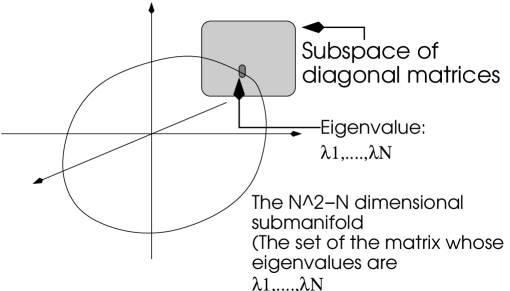
Figure 17: This figure shows the space of the hermitian $N^{2}$ dimensional matrix. The submanifold show the orbit of the unitary transformation of the diagonal matrix $diag(\lambda_{1},\cdots,\lambda_{N})$.

Now, we consider the $N^{2}-N$ dimensional submanifold, depicted by the ’loop’ in the above picture, of the manifold of the entire $N^{2}$ dimensional matrix $M$. This manifold can be expressed by $N$ parameters, $\lambda_{1}\cdots\lambda_{N}$. We consider the effect of the integration with respect to the unitary matrix. In order to understand this effect, we consider the infinitesimal transformation with respect to the unitary matrix. Let $U$ be $U=1+i\epsilon$. The bases of infinitesimal matrix (id est, the Lie algebra of the unitary group) are $u_{ij}=\epsilon_{ij}E_{ij}+\epsilon^{\dagger}_{ij}E_{ji}$ (where $E_{ij}$ is a matrix whose $(i,j)$ component is $1$ and other components are 0). Taking the commutator, we obtain

$$[diag(\lambda_{1},\cdots,\lambda_{N}),u_{ij}]=-\epsilon_{ij}E_{ij}(\lambda_{i}-\lambda_{j})+\epsilon^{\dagger}_{ij}E_{ji}(\lambda_{i}-\lambda_{j}),$$ (B.3)

Therefore, the contribution to the measure is $(\lambda_{i}-\lambda_{j})^{2}$. We take all the products of $i,j(i<j)$, then the integration of the unitary matrix gives $h(\lambda_{1},\cdots,\lambda_{N})=\prod_{i<j}(\lambda_{i}-\lambda_{j})^{2}$. We finally obtain our desired result
$\displaystyle d^{N^{2}}M=\prod_{i}d\lambda_{i}\prod_{i<j}(\lambda_{i}-\lambda_{j})^{2}dU_{ij}.$ (B.4)

B.2 Proof of (4.52)

This appendix is devoted to the computation of the action of $osp(1|32,R)$ cubic matrix model. The computation of the bosonic part $tr(m^{a}m^{b}m^{c})Tr(T^{a}[T^{b},T^{c}])$ is especially tedious, and this appendix provides the technique to deal with this computation. In this computation, it is easier to rely on the color indices, rather than to adopt large $N$ representation. The bosonic $32\times 32$ matrices $m^{a}$ are expressed in terms of the basis of the gamma matrices

$$m^{a}=u^{a}_{\mu}\Gamma^{\mu}+\frac{1}{2}u^{a}_{\mu_{1}\mu_{2}}\Gamma^{\mu_{1}\mu_{2}}+\frac{1}{5!}u^{a}_{\mu_{1}\cdots\mu_{5}}\Gamma^{\mu_{1}\cdots\mu_{5}}.$$ (B.5)

We work out the computation of the trace $tr(m^{a}m^{b}m^{c})$ in terms of the coefficients of gamma matrix representation, and the properties in the Appendix. A.2 play an essential role in the analysis.

• The property in Appendix. A.2.5 indicates that all we have to consider is the coefficients of ${\bf 1}_{32\times 32}$ in the product $m^{a}m^{b}m^{c}$, because

  $$tr(\Gamma^{\mu})=tr(\Gamma^{\mu_{1}\mu_{2}})=tr(\Gamma^{\mu_{1}\mu_{2}\mu_{3}})=tr(\Gamma^{\mu_{1}\cdots\mu_{4}})=tr(\Gamma^{\mu_{1}\cdots\mu_{5}})=0.$$ (B.6)

• When we consider the product of the gamma matrices, we utilize the formula in Sec. A.2.3. We have a table of what rank of gamma matrices emerge in the product of two gamma matrices. For example, The product $\Gamma^{\mu_{1}\mu_{2}}\Gamma^{\nu_{1}\nu_{2}}$ produces the gamma matrices of rank 0,2,4. Multiplying another elements $m^{c}\in sp(32)$, only the term $\frac{1}{2!}u^{c}_{\mu_{1}\mu_{2}}\Gamma^{\mu_{1}\mu_{2}}$ contribute to the trace $tr(m^{a}m^{b}m^{c})$ because of the property mentioned in the previous item.

We adopt a new abbreviation $(xyz)$, which means

$$(xyz)=\textrm{the terms emerging from }\frac{1}{x!y!z!}u^{a}_{\mu_{1}\cdots\mu_{x}}u^{b}_{\nu_{1}\cdots\nu_{y}}u^{c}_{\rho_{1}\cdots\rho_{z}}tr(\Gamma^{\mu_{1}\cdots\mu_{x}}\Gamma^{\nu_{1}\cdots\nu_{y}}\Gamma^{\rho_{1}\cdots\rho_{z}}),$$

where $x,y,z=1,2,5$ because we are considering $osp(1|32,R)$ matrix model. Based on the above prescription, the candidate of the nonvanishing terms are as follows:

$$(112),(155),(222),(255),(555).$$ (B.7)

The bosonic part of the action can be written as

$$I_{b} = -\frac{f_{abc}}{2g^{2}}tr(m^{a}m^{b}m^{c})$$ (B.8)

$$= -\frac{f_{abc}}{2g^{2}}tr((112)+(155)+(222)+(255)+(555)).$$

We compute these terms one by one.

(112) terms

.
In the computation of these terms, we must be cautions about the following point: in picking up the term $(xyz)$, we must take into account where we have picked up the $x$ (or $y$, $z$) term. In this case, we must consider the sum

$$(112) = \frac{1}{2!}(u^{a}_{\mu_{1}}u^{b}_{\nu_{1}}u^{c}_{\rho_{1}\rho_{2}}tr(\Gamma^{\mu_{1}}\Gamma^{\nu_{1}}\Gamma^{\rho_{1}\rho_{2}})+u^{a}_{\mu_{1}}u^{b}_{\nu_{1}\nu_{2}}u^{c}_{\rho_{1}}tr(\Gamma^{\mu_{1}}\Gamma^{\nu_{1}\nu_{2}}\Gamma^{\rho_{1}})+u^{a}_{\mu_{1}mu_{2}}u^{b}_{\nu_{1}}u^{c}_{\rho_{1}}tr(\Gamma^{\mu_{1}\mu_{2}}\Gamma^{\nu_{1}}\Gamma^{\rho_{1}}))$$ (B.9)

$$= \frac{1}{2!}u^{a}_{\mu_{1}}u^{b}_{\nu_{1}}u^{c}_{\rho_{1}\rho_{2}}tr(\Gamma^{\mu_{1}}\Gamma^{\nu_{1}}\Gamma^{\rho_{1}\rho_{2}}+\Gamma^{\nu_{1}}\Gamma^{\rho_{1}\rho_{2}}\Gamma^{\mu_{1}}+\Gamma^{\rho_{1}\rho_{2}}\Gamma^{\mu_{1}}\Gamma^{\nu_{1}})$$

$$= \frac{3}{2!}u^{a}_{\mu_{1}}u^{b}_{\nu_{1}}u^{c}_{\rho_{1}\rho_{2}}tr(\Gamma^{\mu_{1}}\Gamma^{\nu_{1}}\Gamma^{\rho_{1}\rho_{2}}),$$

where we have utilized the cyclic symmetry of the trace with respect to the gamma matrices. The formula of the product of the gamma matrices (A.2.3) indicates that

$$tr(\Gamma^{\mu_{1}}\Gamma^{\nu_{1}}\Gamma^{\rho_{1}\rho_{2}})=tr((\Gamma^{\mu_{1}\mu_{2}}+\eta^{\mu_{1}\mu_{2}})\Gamma^{\rho_{1}\rho_{2}})=tr(-2\eta^{\mu_{1}\rho_{1}}\eta^{\nu_{1}\rho_{2}})=-64\eta^{\mu_{1}\rho_{1}}\eta^{\nu_{1}\rho_{2}}.$$ (B.10)

Thus we complete the computation of the (112) term

$$(112)=-96u^{a}_{\mu_{1}}u^{b}_{\nu_{1}}u^{c\mu_{1}\nu_{1}}.$$ (B.11)

(155) terms

.
We perform a computation similar to the case of the (112) term:

$$(155) = \frac{1}{(5!)^{2}}(u^{a}_{\mu_{1}}u^{b}_{\nu_{1}\cdots\nu_{5}}u^{c}_{\rho_{1}\cdots\rho_{5}}tr(\Gamma^{\mu_{1}}\Gamma^{\nu_{1}\cdots\nu_{5}}\Gamma^{\rho_{1}\cdots\rho_{5}})+u^{a}_{\mu_{1}\cdots\mu_{5}}u^{b}_{\nu_{1}}u^{c}_{\rho_{1}\cdots\rho_{5}}tr(\Gamma^{\mu_{1}\cdots\mu_{5}}\Gamma^{\nu_{1}}\Gamma^{\rho_{1}\cdots\rho_{5}})$$ (B.12)

$$+ u^{a}_{\mu_{1}\cdots\mu_{5}}u^{b}_{\nu_{1}\cdots\nu_{5}}u^{c}_{\rho_{1}}tr(\Gamma^{\mu_{1}\cdots\mu_{5}}\Gamma^{\nu_{1}\cdots\nu_{5}}\Gamma^{\rho_{1}}))$$

$$= \frac{1}{(5!)^{2}}u^{a}_{\mu_{1}}u^{b}_{\nu_{1}\cdots\nu_{5}}u^{c}_{\rho_{1}\cdots\rho_{5}}tr(\Gamma^{\mu_{1}}\Gamma^{\nu_{1}\cdots\nu_{5}}\Gamma^{\rho_{1}\cdots\rho_{5}}+\Gamma^{\rho_{1}\cdots\rho_{5}}\Gamma^{\mu_{1}}\Gamma^{\nu_{1}\cdots\nu_{5}}+\Gamma^{\nu_{1}\cdots\nu_{5}}\Gamma^{\rho_{1}\cdots\rho_{5}}\Gamma^{\mu_{1}})$$

$$= \frac{3}{(5!)^{2}}u^{a}_{\mu_{1}}u^{b}_{\nu_{1}\cdots\nu_{5}}u^{c}_{\rho_{1}\cdots\rho_{5}}tr(\Gamma^{\mu_{1}}\Gamma^{\nu_{1}\cdots\nu_{5}}\Gamma^{\rho_{1}\cdots\rho_{5}}).$$

The biggest difference from the previous case is that the nonvanishing term emerges due to the dual of the gamma matrices:

$$tr(\Gamma^{\mu_{1}}\Gamma^{\nu_{1}\cdots\nu_{5}}\Gamma^{\rho_{1}\cdots\rho_{5}})=tr(\Gamma^{\mu_{1}\nu_{1}\cdots\nu_{5}}\Gamma^{\rho_{1}\cdots\rho_{5}})=\frac{-1}{5!}tr(\epsilon^{\mu_{1}\nu_{1}\cdots\nu_{5}\chi_{1}\cdots\chi_{5}}\Gamma_{\chi_{1}\cdots\chi_{5}}\Gamma^{\rho_{1}\cdots\rho_{5}})$$

$$= \frac{-1}{5!}tr(\epsilon^{\mu_{1}\nu_{1}\cdots\nu_{5}\chi_{1}\cdots\chi_{5}}5!\eta_{\chi_{1}}^{\rho_{1}}\cdots\eta_{\chi_{5}}^{\rho_{5}})=-32\epsilon^{\mu_{1}\nu_{1}\cdots\nu_{5}\rho_{1}\cdots\rho_{5}}.$$

Therefore the final result is obtained by

$$(155)=-\frac{1}{150}u^{a}_{\mu_{1}}u^{b}_{\nu_{1}\cdots\nu_{5}}u^{c}_{\rho_{1}\cdots\rho_{5}}\epsilon^{\mu_{1}\nu_{1}\cdots\nu_{5}\rho_{1}\cdots\rho_{5}}.$$ (B.14)

(222) terms

.
This term emerges from the choice that we pick up $\frac{1}{2!}u_{\mu_{1}\mu_{2}}\Gamma^{\mu_{1}\mu_{2}}$ from all of $m^{a},m^{b},m^{c}$. The difference from the previous two cases is that we do not have to consider the number of the ways to pick up the term (222). The contribution is therefore

$$\frac{1}{(2!)^{3}}u^{a}_{\mu_{1}\mu_{2}}u^{b}_{\nu_{1}\nu_{2}}u^{c}_{\rho_{1}\rho_{2}}tr(\Gamma^{\mu_{1}\mu_{2}}\Gamma^{\nu_{1}\nu_{2}}\Gamma^{\rho_{1}\rho_{2}}).$$ (B.15)

We likewise compute the gamma matrices, so that we obtain

$$tr(\Gamma^{\mu_{1}\mu_{2}}\Gamma^{\nu_{1}\nu_{2}}\Gamma^{\rho_{1}\rho_{2}})=tr((\Gamma^{\mu_{1}\mu_{2}\nu_{1}\nu_{2}}-4{\eta^{[\mu_{1}}}^{[\nu_{1}}{\Gamma^{\mu_{2}]}}^{\nu_{2}]}-2{\eta^{[\mu_{1}}}^{[\nu_{1}}{\eta^{\mu_{2}]}}^{\nu_{2}]})\Gamma^{\rho_{1}\rho_{2}})$$ (B.16)

$$= tr(8{\eta^{[\mu_{1}}}^{[\nu_{1}}{\eta^{\mu_{2}]}}^{[\rho_{1}}{\eta^{\nu_{2}]}}^{\rho_{2}]}),$$

where the bracket $[\mu_{1}\mu_{2}\cdots]$ represents the anti-symmetry of the indices (for example $P_{[\mu_{1}\mu_{2}]}=\frac{1}{2}(P_{\mu_{1}\mu_{2}}-P_{\mu_{2}\mu_{1}})$), but it is not necessary to write explicitly this awkward mark because the anti-symmetry is obvious. These indices contract with the antisymmetric indices of $u^{a}_{\mu_{1}\cdots}$. The final result is obtained by

$$(222)=32u^{a}_{\mu_{1}\mu_{2}}{u^{b\mu_{1}}}_{\nu_{1}}u^{c\mu_{2}\nu_{1}}.$$ (B.17)

(255) terms

.
We only repeat the similar procedure, and we proceed rather quickly. The contribution of these terms is

$$\frac{3}{2!(5!)^{2}}u^{a}_{\mu_{1}\mu_{2}}u^{b}_{\nu_{1}\cdots\nu_{5}}u^{c}_{\rho_{1}\cdots\rho_{5}}tr(\Gamma^{\mu_{1}\mu_{2}}\Gamma^{\nu_{1}\cdots\nu_{5}}\Gamma^{\rho_{1}\cdots\rho_{5}}).$$ (B.18)

Computing the gamma matrices similarly,

$$\Gamma^{\mu_{1}\mu_{2}}\Gamma^{\nu_{1}\cdots\nu_{5}}\Gamma^{\rho_{1}\cdots\rho_{5}}=-10\eta^{\mu_{1}\nu_{1}}\Gamma^{\mu_{2}\nu_{2}\cdots\nu_{5}}\Gamma^{\rho_{1}\cdots\rho_{5}}$$ (B.19)

$$= -1200\eta^{\mu_{1}\nu_{1}}\eta^{\mu_{2}\rho_{1}}\eta^{\nu_{2}\rho_{2}}\eta^{\nu_{3}\rho_{3}}\eta^{\nu_{4}\rho_{4}}\eta^{\nu_{5}\rho_{5}}.$$

Therefore, the final result is

$$(255)=-4u^{a}_{\mu_{1}\mu_{2}}{u^{b\mu_{1}}}_{\nu_{1}\cdots\nu_{4}}u^{c\mu_{2}\nu_{1}\cdots\nu_{4}}.$$ (B.20)

(555) terms

.
The contribution is obtained by

$$\frac{1}{(5!)^{3}}u^{a}_{\mu_{1}\cdots\mu_{5}}u^{b}_{\nu_{1}\cdots\nu_{5}}u^{c}_{\rho_{1}\cdots\rho_{5}}tr(\Gamma^{\mu_{1}\cdots\mu_{5}}\Gamma^{\nu_{1}\cdots\nu_{5}}\Gamma^{\rho_{1}\cdots\rho_{5}}).$$ (B.21)

The product of the gamma matrices is computed to be

$$\Gamma^{\mu_{1}\cdots\mu_{5}}\Gamma^{\nu_{1}\cdots\nu_{5}}\Gamma^{\rho_{1}\cdots\rho_{5}}=\frac{200}{5!}\eta^{\mu_{1}\nu_{1}}\eta^{\mu_{2}\nu_{2}}\epsilon^{\mu_{3}\mu_{4}\mu_{5}\nu_{3}\nu_{4}\nu_{5}\chi_{1}\cdots\chi_{5}}\Gamma_{\chi_{1}\cdots\chi_{5}}\Gamma^{\rho_{1}\cdots\rho_{5}}$$ (B.22)

$$= 200\eta^{\mu_{1}\nu_{1}}\eta^{\mu_{2}\nu_{2}}\epsilon_{\mu_{3}\mu_{4}\mu_{5}\nu_{3}\nu_{4}\nu_{5}\rho_{1}\cdots\rho_{5}}.$$

The result is therefore,

$$(555)=\frac{1}{270}u^{a}_{\mu_{1}\cdots\mu_{5}}{u^{b\mu_{1}\mu_{2}}}_{\nu_{3}\nu_{4}\nu_{5}}u^{c}_{\rho_{1}\cdots\rho_{5}}\epsilon^{\mu_{3}\mu_{4}\mu_{5}\nu_{3}\nu_{4}\nu_{5}\rho_{1}\cdots\rho_{5}}.$$ (B.23)

The conclusion of this lengthy computation is summarized as

$$(112) = -96u^{a}_{\mu_{1}}u^{b}_{\nu_{1}}u^{c\mu_{1}\nu_{1}},$$

$$(155) = -\frac{1}{150}u^{a}_{\mu_{1}}u^{b}_{\nu_{1}\cdots\nu_{5}}u^{c}_{\rho_{1}\cdots\rho_{5}}\epsilon^{\mu_{1}\nu_{1}\cdots\nu_{5}\rho_{1}\cdots\rho_{5}},$$

$$(222) = 32u^{a}_{\mu_{1}\mu_{2}}{u^{b\mu_{1}}}_{\nu_{1}}u^{c\mu_{2}\nu_{1}},$$

$$(255) = -4u^{a}_{\mu_{1}\mu_{2}}{u^{b\mu_{1}}}_{\nu_{1}\cdots\nu_{4}}u^{c\mu_{2}\nu_{1}\cdots\nu_{4}},$$

$$(555) = \frac{1}{270}u^{a}_{\mu_{1}\cdots\mu_{5}}{u^{b\mu_{1}\mu_{2}}}_{\nu_{3}\nu_{4}\nu_{5}}u^{c}_{\rho_{1}\cdots\rho_{5}}\epsilon^{\mu_{3}\mu_{4}\mu_{5}\nu_{3}\nu_{4}\nu_{5}\rho_{1}\cdots\rho_{5}}.$$

We next examine the fermionic part of this action. However, the computation of its contribution is trivial:

$$I_{f} = -\frac{f_{abc}}{2g^{2}}(-3i{\bar{\psi}^{a}}m^{b}\psi^{c})$$ (B.24)

$$= \frac{3if_{abc}}{2g^{2}}({\bar{\psi}^{a}}\Gamma^{\mu_{1}}u^{b}_{\mu_{1}}\psi^{c}+\frac{1}{2!}{\bar{\psi}^{a}}\Gamma^{\mu_{1}\mu_{2}}u^{b}_{\mu_{1}\mu_{2}}\psi^{c}+\frac{1}{5!}{\bar{\psi}^{a}}\Gamma^{\mu_{1}\cdots\mu_{5}}u^{b}_{\mu_{1}\cdots\mu_{5}}\psi^{c}).$$

We are now finished with the computation of the action in terms of the components $\{u_{X}\}$. This is a description in terms of 11 dimensional indices. One of the problems we should tackle with is the correspondence between this cubic matrix theory and the existing 10 dimensional matrix theory such as IKKT model. For this purpose, it is more convenient to express the indices for 10 dimensions. Rewriting the above terms in terms of the variables (4.49), we obtain a final result.

B.3 Propagator of the action (4.4) $\sim$ (4.111)

This section is devoted to the investigation of the Feynman rules of the action (4.4) $\sim$ (4.111). Most of the Feynman rules are trivially read off from the Lagrangian, however the non-trivial problem is the propagator among the fields $W$, $A_{i}$ and $C_{ij}$. This is due to the kinetic term

$$\frac{1}{g^{2}}Tr_{N\times N}(96W\partial_{i}A^{(-)i}-96A^{(-)}_{i}\partial_{j}C^{ij}),$$ (B.25)

in which the vector fields $A^{(-)}_{i}$ are connected with both $W$ and $C_{ij}$ fields. We would like to investigate the Feynman diagram among the three fields $W$, $A^{(-)}_{i}$ and $C_{ij}$. For simplicity, we omit an awkward coefficient $\frac{96}{g^{2}}$. Then, the Lagrangian in question is

$$I_{WAC}=-W\partial_{i}A^{(-)}_{i}+A^{(-)}_{i}\partial_{j}C^{ij}.$$ (B.26)

• First, we disprove the existence of the propagator $\langle A^{(-)}_{i}C^{ij}\rangle$. This stems from the gauge freedom of the field $C^{ij}$. As is easily read off from the action (B.26), $C^{ij}$ is invariant under the transformation

  $$C^{ij}\to C^{ij}+\partial_{k}\chi^{ijk},$$ (B.27)

  where the quantity $\chi^{ijk}$ is anti-symmetric with respect to the exchange of the indices. Therefore, the propagators $\langle A^{(-)}_{i}C^{ij}\rangle$ do not exist in this theory.

• We next consider the propagator $\langle WA^{(-)}_{i}\rangle$. This is understood by first integrating out the fields $C^{ij}$. Since this action is linear with respect to $C^{ij}$, this is tantamount to solving the classical Euler-Lagrange equation with respect to $C^{ij}$:

  $$\partial_{k}(\frac{\partial I_{WAC}}{\partial(\partial_{k}C^{ij})})-\frac{\partial I_{WAC}}{\partial C^{ij}}=\partial_{[j}A^{(-)}_{i]}=0.$$ (B.28)

  Note that the indices are anti-symmetrized because we have solved the Euler-Lagrange equation with respect to $C^{ij}$. The gauge field $A^{(-)}_{i}$ is thus constrained to be

  $$\partial_{i}A^{(-)}_{j}-\partial_{j}A^{(-)}_{i}=0,\Rightarrow{{}^{\exists}\lambda}\textrm{ s.t. }A^{(-)}_{i}=\partial_{i}\lambda.$$ (B.29)

  Substituting (B.29) into the action (B.26), the action is

  $$I_{WAC}=-W\partial_{i}\partial^{i}\lambda.$$ (B.30)

  This indicates that the propagator for $W$ and $\lambda$ is $\langle W\lambda\rangle\sim\frac{1}{p^{2}}$. Therefore, we obtain a propagator for $W$ and $A^{(-)}_{i}$:

  $$\langle WA^{(-)}_{i}\rangle\sim\frac{p_{i}}{p^{2}}.$$ (B.31)

B.4 Disproof of the existence of the perturbative propagators $\langle WW\rangle$ and $\langle A^{(-)}_{i}A^{(-)}_{j}\rangle$

In this subsection, we develop a disproof of such propagators as $\langle WW\rangle$ and $\langle A^{(-)}_{i}A^{(-)}_{j}\rangle$ at a perturbative level. This statement is verified more generally, and we use a rather abstract expression. The bosonic terms in $osp(1|32,R)$ cubic matrix theory is distinguished into the following two groups.

• $U_{e}$ denotes the fields of even rank with respect to 10 dimensional indices. Id est, we mean the fields $W$, $C_{ij}$ and $H_{ijkl}$.

• $U^{(\pm)}_{o}$ denotes the fields of odd rank in terms of 10 dimensional indices with plus (or minus) chirality.

  • $U^{(+)}_{i}$ denotes $A^{(+)}_{i}$ or $I^{(+)}_{i_{1}\cdots i_{5}}$.

  • $U^{(-)}_{i}$ denotes $A^{(-)}_{i}$ or $I^{(-)}_{i_{1}\cdots i_{5}}$.

We have expanded this cubic matrix theory around the classical solution (4.105) and considered the following mapping

$$[A^{(+)}_{i},X]\Rightarrow-i\partial_{i}X+[a^{(+)}_{i},X].$$ (B.32)

Therefore, the action with the kinetic terms introduced by this mapping is abstractly expressed as follows:

$$I=\{(\partial U_{e})U^{(-)}_{o}+(\partial{\bar{\psi}_{L}})\psi_{L}\}+(U_{e}U^{(+)}_{o}U^{(-)}_{o}+{\bar{\psi}_{L}}U^{(+)}_{o}\psi_{L}+{\bar{\psi}_{R}}U^{(-)}_{o}\psi_{R}+U^{3}_{e}+{\bar{\psi}_{L}}U_{e}\psi_{R}).$$ (B.33)

• We can in general verify that the product of plural fields of the same chirality (such as $U^{(+)}_{o}U^{(+)}_{o}$ or $U^{(-)}_{o}U^{(-)}_{o}$) never emerges in this cubic action. This can be verified by noting the structure of gamma matrices. For example, suppose that such terms as $U^{(+)}_{o}U^{(+)}_{o}U^{X}$ emerges in the bosonic part of the cubic action. This would appear in the action,

  $$Tr_{N\times N}(U^{(+)}_{o}U^{(+)}_{o}U^{X})tr(\Gamma^{o}(1+\Gamma^{\sharp})\Gamma^{o}(1+\Gamma^{\sharp})\Gamma^{X}),$$ (B.34)

  where $\Gamma^{o}$ denotes the gamma matrices of odd rank in terms of 10 dimensional indices, such as $\Gamma^{i}$ or $\Gamma^{ijklm}$. Be careful about the structure of the gamma matrices. Noting the Clifford algebra $\Gamma^{i}\Gamma^{\sharp}+\Gamma^{\sharp}\Gamma^{i}=0$, this gamma matrix is shown to vanish:

  $$\Gamma^{o}(1+\Gamma^{\sharp})\Gamma^{o}(1+\Gamma^{\sharp})\Gamma^{X}=\Gamma^{o}\Gamma^{o}(1-\Gamma^{\sharp})(1+\Gamma^{\sharp})\Gamma^{X}=0.$$ (B.35)

  Therefore, The bosonic part is restricted to be $U^{(+)}_{o}U^{(-)}_{o}U_{e}$ or $U_{e}^{3}$.

• For the same reason, the kinetic term is restricted to be $(\partial U^{(-)}_{o})U_{e}$ since the kinetic terms emerge from the expansion around the classical solution (4.105)

• The fermionic terms is restricted to be of the form ${\bar{\psi}_{L}}U^{(+)}_{o}\psi_{L}$, ${\bar{\psi}_{R}}U^{(-)}_{o}\psi_{R}$ or ${\bar{\psi}_{L}}U_{e}\psi_{R}$, which is understood from the properties (A.14).

In order to develop perturbative argument, we assign a following charge, and perform the correspondence rescaling.

• $U_{e}$, $U^{(+)}_{o}$ and $U^{(-)}_{o}$ are assigned the charge $1$, $0$ and $-1$ respectively. Id est, the scaling is $U^{e}\to e^{\lambda}U_{e}$, $U^{(+)}_{o}\to U^{(+)}_{o}$ and $U^{(-)}_{o}\to U^{(-)}e^{-\lambda}$.

• $\psi_{L}$ and $\psi_{R}$ are assigned charge 0 and $\frac{1}{2}$ respectively. Id est, the scaling is $\psi_{L}\to\psi_{L}$ and $\psi_{R}\to\psi_{R}e^{\frac{\lambda}{2}}$.

Following these scaling rules, this action is thus rescaled as follows:

$$I=\{(\partial U_{e})U^{(-)}_{o}+(\partial{\bar{\psi}_{L}})\psi_{L}\}+(U_{e}U^{(+)}_{o}U^{(-)}_{o}+{\bar{\psi}_{L}}U^{(+)}_{o}\psi_{L}+{\bar{\psi}_{R}}U^{(-)}_{o}\psi_{R})+(U^{3}_{e}e^{3\lambda})+({\bar{\psi}_{L}}U_{e}\psi_{R}e^{\frac{3\lambda}{2}}).$$ (B.36)

This action possesses only the propagators $\langle\psi_{L}\psi_{L}\rangle$ and $\langle U^{(-)}_{o}U_{e}\rangle$ at tree level. Other propagators are induced by the multi-loop effect. And the vertices in this action and their charges are given below.

Figure 18: The possible vertices of this Lagrangian and their charge.

If the induced propagators of $\langle U_{e}U_{e}\rangle$, $\langle U^{(-)}_{o}U^{(-)}_{o}\rangle$ and $\langle\psi_{R}\psi_{R}\rangle$ are to exist, they can be constructed by the combination of those vertices. The charge of $U_{e}U_{e}$, $U^{(-)}_{o}U^{(-)}_{o}$ and $\psi_{R}\psi_{R}$ is $+2,-2,+1$, respectively. Therefore, the possible charges of these induced propagators are listed below.

propagator	$\langle U_{e}U_{e}\rangle$	$\langle U^{(-)}_{o}U^{(-)}_{o}\rangle$	$\psi_{R}\psi_{R}$
charge	$2+3n+\frac{3m}{2}$	$-2+3n+\frac{3m}{2}$	$1+3n+\frac{3m}{2}$

where $n$ and $m$ are the number of the vertices $U_{e}-U_{e}-U_{e}$ and $\psi_{L}-\psi_{R}-U_{e}$. Since the propagators at tree level is of charge 0, the propagators do not contribute to the charge of the induced propagators. The point is that, even if we consider the multi-loop effect, the charge of these propagators increases by the multiple of $3$ or $\frac{3}{2}$. Thus, it is impossible to construct the propagators of these fields with charge 0 no matter how we combine the propagators and the vertices.

If the charge of the propagators is nonzero, these induced propagators vanishes when we integrate out the parameter $\lambda$. Therefore, such propagators as $\langle WW\rangle$ or $\langle A^{(-)}_{i}A^{(-)}_{j}\rangle$ cannot emerge by the perturbative multi-loop effect.

B.5 Explicit form of the $gl(1|32,R)\otimes gl(N,R)$ gauged cubic action

This section is devoted to executing the tedious computation of the $gl(1|32,R)\otimes gl(N,R)$ gauged cubic matrix theory. Especially we focus on the bosonic part $tr(m^{a}m^{b}m^{c})$, because this is the most difficult and cumbersome to compute. We rely on the expression of color indices. We first express the trace in terms of the basis of the gamma matrices:

$$m^{a}=u^{a}{\bf 1}+u^{a}_{\mu_{1}}\Gamma^{\mu_{1}}+\frac{1}{2!}u^{a}_{\mu_{1}\mu_{2}}\Gamma^{\mu_{1}\mu_{2}}+\frac{1}{3!}u^{a}_{\mu_{1}\mu_{2}\mu_{3}}\Gamma^{\mu_{1}\mu_{2}\mu_{3}}+\frac{1}{4!}u^{a}_{\mu_{1}\cdots\mu_{4}}\Gamma^{\mu_{1}\cdots\mu_{4}}+\frac{1}{5!}u^{a}_{\mu_{1}\cdots\mu_{5}}\Gamma^{\mu_{1}\cdots\mu_{5}}.$$ (B.37)

And whether these coefficients appear as a commutator or anti-commutator affects the physics crucially. Let us investigate the structure of the action from another point of view. Considering the correspondence of the super Lie algebra $gl(1|32,R)$ with $u(1|16,16)$, we have in the previous section noted that $gl(1|32,R)$ can be expressed by the direct sum $gl(1|32,R)={\cal H}\oplus{\cal A}$. The following properties play an essential role in the investigation of the action, especially the cumbersome bosonic part. For $H_{1},H_{2},H_{3}\in{\cal H}$ and $A_{1},A_{2},A_{3}\in{\cal A}$,

$$(1)Str(H_{1}H_{2}H_{3})=\frac{1}{2}Str(H_{1}[H_{2},H_{3}]),\hskip 5.69054pt(2)Str(H_{1}H_{2}A_{3})=\frac{1}{2}Str(H_{1}\{H_{2},A_{3}\}),\hskip 5.69054pt$$

$$(3)Str(H_{1}A_{2}A_{3})=\frac{1}{2}Str(H_{1}[A_{2},A_{3}])\hskip 5.69054pt(4)Str(A_{1}A_{2}A_{3})=\frac{1}{2}Str(A_{1}\{A_{2},A_{3}\}).$$ (B.38)

(Proof) This relationship is readily verified by noting the commutation and anti-commutation relationships of the two different representations of $osp(1|32,R)$, as we have seen in (5.42). Noting these relationships, we readily obtain the following property:

$$\textrm{For }H\in{\cal H}\textrm{ and }A\in{\cal A},Str(HA)=0.$$ (B.39)

This can be verified by noting that $G^{2}=-1$ and that the cyclic rule holds true of the supertrace:

$$Str(HA)=Str({{}^{T}A}{{}^{T}H})=-Str({{}^{T}A}G^{2}{{}^{T}H})=Str({{}^{T}A}GHG)=Str(GAHG)=-Str(AH)=-Str(HA).$$

$Str(HA)$ satisfies $Str(HA)=-Str(HA)$, and thus this is shown to vanish.

Utilizing the relationships (5.42) and (B.39), the proof of (B.38) goes as follows:

1. $Str(H_{1}H_{2}H_{3})=\frac{1}{2}Str(H_{1}([H_{2},H_{3}]+\{H_{2},H_{3}\}))=\frac{1}{2}Str(H_{1}[H_{2},H_{3}])+\frac{1}{2}Str(H_{1}{\cal A})=\frac{1}{2}Str(H_{1}[H_{2},H_{3}])$,

2. $Str(H_{1}H_{2}A_{3})=\frac{1}{2}Str(H_{1}([H_{2},A_{3}]+\{H_{2},A_{3}\}))=\frac{1}{2}Str(H_{1}{\cal A})+\frac{1}{2}Str(H_{1}\{H_{2},A_{3}\})=\frac{1}{2}Str(H_{1}\{H_{2},A_{3}\})$,

3. $Str(H_{1}A_{2}A_{3})=\frac{1}{2}Str(H_{1}([A_{2},A_{3}]+\{A_{2},A_{3}\}))=\frac{1}{2}Str(H_{1}[A_{2},A_{3}])+\frac{1}{2}Str(H_{1}{\cal A})=\frac{1}{2}Str(H_{1}[A_{2},A_{3}])$,

4. $Str(A_{1}A_{2}A_{3})=\frac{1}{2}Str(A_{1}([A_{2},A_{3}]+\{A_{2},A_{3}\}))=\frac{1}{2}Str(A_{1}{\cal H})+\frac{1}{2}Str(A_{1}\{A_{2},A_{3}\})=\frac{1}{2}Str(A_{1}\{A_{2},A_{3}\})$.

These completes the proof of the properties (B.38). (Q.E.D.)

Now let us separate the components of $gl(1|32,R)$ into the subalgebras ${\cal H}$ and ${\cal A}$. The element $M^{a}\in gl(1|32,R)$ can be separated as

$$M^{a}=H^{a}+A^{a}=\left(\begin{array}[]{cc}m^{a}_{1}&\psi^{a}_{1}\\ i{\bar{\psi}_{1}}^{a}&0\end{array}\right)+\left(\begin{array}[]{cc}m^{a}_{2}&\psi^{a}_{2}\\ -i{\bar{\psi}_{2}}^{a}&v^{a}\end{array}\right),$$ (B.44)

where $m_{1},m_{2},\psi_{1},\psi_{2}$ are defined in the previous section. Then, the action is rewritten as

$$I = \frac{1}{g^{2}}Str(M^{a}M^{b}M^{c})Tr(T^{a}T^{b}T^{c})=\frac{1}{2g^{2}}Str((H^{a}+A^{a})(H^{b}+A^{b})(H^{c}+A^{c}))(Tr(T^{a}[T^{b},T^{c}])+Tr(T^{a}\{T^{b},T^{c}\}))$$ (B.45)

$$\stackrel{{\scriptstyle(\ref{AZ53distinguish})}}{{=}} \frac{1}{4g^{2}}(Str(H^{a}[H^{b},H^{c}])+Str(H^{a}[A^{b},A^{c}]))Tr(T^{a}[T^{b},T^{c}])$$

$$+ \frac{1}{4g^{2}}(Str(H^{a}\{H^{b},A^{c}\})+Str(A^{a}\{A^{b},A^{c}\}))Tr(T^{a}\{T^{b},T^{c}\})$$

$$\stackrel{{\scriptstyle(\ref{AZ52structureconst})}}{{=}} \frac{f_{abc}}{4g^{2}}(Str(H^{a}[H^{b},H^{c}])+Str(H^{a},[A^{b},A^{c}]))+\frac{d_{abc}}{4g^{2}}(Str(H^{a}\{H^{b},A^{c}\})+Str(A^{a}\{A^{b},A^{c}\}))$$

$$= \frac{f_{abc}}{2g^{2}}(Str(H^{a}H^{b}H^{c})+Str(H^{a}A^{b}A^{c}))+\frac{d_{abc}}{2g^{2}}(Str(H^{a}H^{b}A^{c})+Str(A^{a}A^{b}A^{c})).$$ (B.46)

We compute the trace $tr(m^{a}m^{b}m^{c})$ according to the same principle as in $osp(1|32,R)$ bosonic part. Since the trace of the gamma matrices is

$$tr(\Gamma^{\mu})=tr(\Gamma^{\mu_{1}\mu_{2}})=tr(\Gamma^{\mu_{1}\mu_{2}\mu_{3}})=tr(\Gamma^{\mu_{1}\cdots\mu_{4}})=tr(\Gamma^{\mu_{1}\cdots\mu_{5}})=0,$$ (B.47)

the goal of the computation of $tr(mmm)$ is to extract the coefficient of ${\bf 1}_{32\times 32}$, and we utilize the formula (A.2.3) for the computation of the gamma matrices. We separate the contribution of the bosonic part $tr(mmm)$ into the following four parts, and we inherit the abbreviation $(xyz)$ from the argument of $osp(1|32,R)$:

$$(xyz)\stackrel{{\scriptstyle def}}{{=}}\textrm{the terms emerging from }\frac{1}{x!y!z!}u^{a}_{\mu_{1}\cdots\mu_{x}}u^{b}_{\mu_{1}\cdots\mu_{y}}u^{c}_{\mu_{1}\cdots\mu_{z}}tr(\Gamma^{\mu_{1}\cdots\mu_{x}}\Gamma^{\mu_{1}\cdots\mu_{y}}\Gamma^{\mu_{1}\cdots\mu_{z}}),$$ (B.48)

where now $x,y,z=0,1,\cdots,5$. The technique of the following computation is totally the same as in $osp(1|32,R)$ cubic model, as was discussed in Appendix. B.2

B.5.1 (F1) terms

We nane the terms emerging from $\frac{f_{abc}}{2g^{2}}Str(H^{a}H^{b}H^{c})$ (F1) terms. We utilize the color indices notation for simplicity, and switch to the large $N$ matrix representation. These terms are attached to the commutator of the basis of $gl(N,R)$, and therefore anti-symmetric with respect to the exchange of the color indices $a\leftrightarrow b$. As we have seen, the bosonic part $m_{1}$ is

$$m^{a}=u^{a}_{\mu_{1}}\Gamma^{\mu_{1}}+\frac{1}{2!}u^{b}_{\mu_{1}\mu_{2}}\Gamma^{\mu_{1}\mu_{2}}+\frac{1}{5!}u^{a}_{\mu_{1}\cdots\mu_{5}}\Gamma^{\mu_{1}\cdots\mu_{5}}.$$ (B.49)

Therefore, the nonvanishing trace is

$$(112),(155),(222),(255),(555),$$ (B.50)

whose computation we do not repeat because we are finished with these computations in the investigation of $osp(1|32,R)$.

B.5.2 (F2) terms

We refer to the terms $\frac{f_{abc}}{2g^{2}}Str(H^{a}A^{b}A^{c})$ as (F2) terms. The nonvanishing trace comes from

$$(134),(233),(244),(335),(345),(445).$$ (B.51)

The fundamental techniques and cautions are already introduced in the analysis of $osp(1|32,R)$, and we proceed rather quickly.

(134) terms

There are 6 ways as to where we should pick up which terms, and the contribution is

$$(134)=\frac{6}{3!4!}u^{a}_{\mu_{1}}u^{b}_{\nu_{1}\nu_{2}\nu_{3}}u^{c}_{\rho_{1}\cdots\rho_{4}}tr(\Gamma^{\mu_{1}}\Gamma^{\nu_{1}\nu_{2}\nu_{3}}\Gamma^{\rho_{1}\cdots\rho_{4}}).$$ (B.52)

On the other hand, the trace of the gamma matrices are computed to be

$$tr(\Gamma^{\mu_{1}}\Gamma^{\nu_{1}\nu_{2}\nu_{3}}\Gamma^{\rho_{1}\cdots\rho_{4}})=tr(\Gamma^{\mu_{1}\nu_{1}\nu_{2}\nu_{3}}\Gamma^{\rho_{1}\cdots\rho_{4}})=24\eta^{\mu_{1}\rho_{1}}\eta^{\nu_{1}\rho_{2}}\eta^{\nu_{2}\rho_{3}}\eta^{\nu_{3}\rho_{4}}.$$ (B.53)

Therefore, the contribution is

$$(134)=32u^{a}_{\mu_{1}}u^{b}_{\nu_{1}\nu_{2}\nu_{3}}u^{c\mu_{1}\nu_{1}\nu_{2}\nu_{3}}.$$ (B.54)

(233) terms

The contribution of (233) term is

$$\frac{3}{2!(3!)^{2}}tr(u^{a}_{\mu_{1}\mu_{2}}u^{b}_{\nu_{1}\cdots\nu_{3}}u^{c}_{\rho_{1}\cdots\rho_{3}}f_{abc}\Gamma^{\mu_{1}\mu_{2}}\Gamma^{\nu_{1}\cdots\nu_{3}}\Gamma^{\rho_{1}\cdots\rho_{3}}).$$ (B.55)

Again, using the formula of the gamma matrices,

$$\Gamma^{\mu_{1}\mu_{2}}\Gamma^{\nu_{1}\cdots\nu_{3}}\Gamma^{\rho_{1}\cdots\rho_{3}}=-6\eta^{\mu_{1}\nu_{1}}\Gamma^{\mu_{2}\nu_{2}\nu_{3}}\Gamma^{\rho_{1}\cdots\rho_{3}}=36\eta^{\mu_{1}\nu_{1}}\eta^{\mu_{2}\rho_{1}}\eta^{\nu_{2}\rho_{2}}\eta^{\nu_{3}\rho_{3}}.$$ (B.56)

Then, the final result is

$$(233)=48u^{a}_{\mu_{1}\mu_{2}}{u^{b\mu_{1}}}_{\nu_{2}\nu_{3}}u^{c\mu_{2}\nu_{2}\nu_{3}}.$$ (B.57)

(244) terms

Again, there are 3 choices with respect to where we should pick up $u_{\mu_{1}\mu_{2}}$ from $m^{a},m^{b},m^{c}$. Then, the contribution is

$$\frac{3}{2!(4!)^{2}}tr(u^{a}_{\mu_{1}\mu_{2}}u^{b}_{\nu_{1}\cdots\nu_{4}}u^{c}_{\rho_{1}\cdots\rho_{4}}f_{abc}\Gamma^{\mu_{1}\mu_{2}}\Gamma^{\nu_{1}\cdots\nu_{4}}\Gamma^{\rho_{1}\cdots\rho_{4}}).$$ (B.58)

The gamma matrices are computed to be

$$\Gamma^{\mu_{1}\mu_{2}}\Gamma^{\nu_{1}\cdots\nu_{4}}\Gamma^{\rho_{1}\cdots\rho_{4}}=-8\eta^{\mu_{1}\nu_{1}}\Gamma^{\mu_{2}\nu_{2}\nu_{3}\nu_{4}}\Gamma^{\rho_{1}\cdots\rho_{4}}=-192\eta^{\mu_{1}\nu_{1}}\eta^{\mu_{2}\rho_{1}}\eta^{\nu_{2}\rho_{2}}\eta^{\nu_{3}\rho_{3}}\eta^{\nu_{4}\rho_{4}}.$$ (B.59)

Then we obtain,

$$(244)=-16u^{a}_{\mu_{1}\mu_{2}}{u^{b\mu_{1}}}_{\nu_{2}\nu_{3}\nu_{4}}u^{c\mu_{2}\nu_{2}\nu_{3}\nu_{4}}.$$ (B.60)

(335) terms

The contribution of this term is

$$\frac{3}{(3!)^{2}5!}tr(u^{a}_{\mu_{1}\cdots\mu_{3}}u^{b}_{\nu_{1}\cdots\nu_{3}}u^{c}_{\rho_{1}\cdots\rho_{5}}f_{abc}\Gamma^{\mu_{1}\cdots\mu_{3}}\Gamma^{\nu_{1}\cdots\nu_{3}}\Gamma^{\rho_{1}\cdots\rho_{5}}).$$ (B.61)

The gamma matrices are computed to be

$$\Gamma^{\mu_{1}\cdots\mu_{3}}\Gamma^{\nu_{1}\cdots\nu_{3}}\Gamma^{\rho_{1}\cdots\rho_{5}}=\Gamma^{\mu_{1}\cdots\mu_{3}\nu_{1}\cdots\nu_{3}}\Gamma^{\rho_{1}\cdots\rho_{5}}=-\frac{1}{5!}\epsilon^{\mu_{1}\cdots\mu_{3}\nu_{1}\cdots\nu_{3}\chi_{1}\cdots\chi_{5}}\Gamma_{\chi^{1}\cdots\chi^{5}}\Gamma^{\rho_{1}\cdots\rho_{5}}$$ (B.62)

$$= -\epsilon^{\mu_{1}\cdots\mu_{3}\nu_{1}\cdots\nu_{3}\rho_{1}\cdots\rho_{5}}.$$

Therefore, the final result is

$$(335)=-\frac{1}{45}(u^{a}_{\mu_{1}\cdots\mu_{3}}u^{b}_{\nu_{1}\cdots\nu_{3}}u^{c}_{\rho_{1}\cdots\rho_{5}}\epsilon^{\mu_{1}\cdots\mu_{3}\nu_{1}\cdots\nu_{3}\rho_{1}\cdots\rho_{5}}).$$ (B.63)

(345) terms

The contribution to this term is

$$\frac{6}{3!4!5!}u^{a}_{\mu_{1}\cdots\mu_{3}}u^{b}_{\nu_{1}\cdots\nu_{4}}u^{c}_{\rho_{1}\cdots\rho_{5}}f_{abc}tr(\Gamma^{\mu_{1}\cdots\mu_{3}}\Gamma^{\nu_{1}\cdots\nu_{4}}\Gamma^{\rho_{1}\cdots\rho_{5}}).$$ (B.64)

On the other hand, the gamma matrices are evaluated to be

$$\Gamma^{\mu_{1}\cdots\mu_{3}}\Gamma^{\nu_{1}\cdots\nu_{4}}\Gamma^{\rho_{1}\cdots\rho_{5}}=12\eta^{\mu_{1}\nu_{1}}\Gamma^{\mu_{2}\mu_{3}\nu_{2}\nu_{3}\nu_{4}}\Gamma^{\rho_{1}\cdots\rho_{5}}=1440\eta^{\mu_{1}\nu_{1}}\eta^{\mu_{2}\rho_{1}}\eta^{\mu_{3}\rho_{2}}\eta^{\nu_{2}\rho_{3}}\eta^{\nu_{3}\rho_{4}}\eta^{\nu_{4}\rho_{5}}.$$ (B.65)

Therefore, the final result is

$$(345)=16u^{a}_{\mu_{1}\cdots\mu_{3}}{u^{b\mu_{1}}}_{\nu_{2}\nu_{3}\nu_{4}}u^{c\mu_{2}\mu_{3}\nu_{2}\nu_{3}\nu_{4}}.$$ (B.66)

(445) terms

The contribution is expressed as

$$\frac{3}{(4!)^{2}5!}tr(u^{a}_{\mu_{1}\cdots\mu_{4}}u^{b}_{\nu_{1}\cdots\nu_{4}}u^{c}_{\rho_{1}\cdots\rho_{5}}f_{abc}(\Gamma^{\mu_{1}\cdots\mu_{4}}\Gamma^{\nu_{1}\cdots\nu_{4}}\Gamma^{\rho_{1}\cdots\rho_{5}})).$$ (B.67)

The multiplication of the gamma matrices is

$$\Gamma^{\mu_{1}\cdots\mu_{4}}\Gamma^{\nu_{1}\cdots\nu_{4}}\Gamma^{\rho_{1}\cdots\rho_{5}}=\frac{16}{5!}\eta^{\mu_{1}\nu_{1}}\epsilon^{\mu_{2}\mu_{3}\mu_{4}\nu_{2}\nu_{3}\nu_{4}\chi_{1}\cdots\chi_{5}}\Gamma_{\chi_{1}\cdots\chi_{5}}\Gamma^{\rho_{1}\cdots\rho_{5}}=16\eta^{\mu_{1}\nu_{1}}\epsilon^{\mu_{2}\mu_{3}\mu_{4}\nu_{2}\nu_{3}\nu_{4}\rho_{1}\cdots\rho_{5}}.$$ (B.68)

Therefore, the contribution is seen to be

$$\frac{1}{45}u^{a}_{\mu_{1}\cdots\mu_{4}}{u^{b\mu_{1}}}_{\nu_{2}\nu_{3}\nu_{4}}u^{c}_{\rho_{1}\cdots\rho_{5}}\epsilon^{\mu_{2}\mu_{3}\mu_{4}\nu_{2}\nu_{3}\nu_{4}\rho_{1}\cdots\rho_{5}}.$$ (B.69)

B.5.3 (D1) terms

We next investigate the terms coming from the contribution $\frac{d_{abc}}{2g^{2}}Str(A^{a}A^{b}A^{c})$. The difference from the previous two cases is that these terms are attached to the anti-commutator of the gamma matrices, so that the result is symmetric with respect to the exchange of the color indices $a\leftrightarrow b$. This term is named ’(D1) term’ after the structure constant $d_{abc}$. The nonvanishing trace of these this term stems from the following terms:

$$(000),(033),(044),(334),(344),(444).$$ (B.70)

(000) terms

The computation of this contribution is trivial:

$$(000)=u^{a}u^{b}u^{c}tr({\bf 1}^{3})=32u^{a}u^{b}u^{c}.$$ (B.71)

(033) terms

This is also trivial, paying attention to where we should pick up the $u{\bf 1}$:

$$(033) = \frac{3}{(3!)^{2}}u^{a}u^{b}_{\nu_{1}\nu_{2}\nu_{3}}u^{c}_{\rho_{1}\rho_{2}\rho_{3}}tr(\Gamma^{\nu_{1}\nu_{2}\nu_{3}}\Gamma^{\rho_{1}\rho_{2}\rho_{3}})$$ (B.72)

$$= \frac{3}{(3!)^{2}}u^{a}u^{b}_{\nu_{1}\nu_{2}\nu_{3}}u^{c}_{\rho_{1}\rho_{2}\rho_{3}}(-32\times 6\eta^{\mu_{1}\nu_{1}}\eta^{\mu_{2}\nu_{2}}\eta^{\mu_{3}\nu_{3}})=-16u^{a}u^{b}_{\mu_{1}\mu_{2}\mu_{3}}u^{c\mu_{1}\mu_{2}\mu_{3}}.$$

(044) terms

Again, we can compute the contribution with ease:

$$(044) = \frac{3}{(4!)^{2}}u^{a}u^{b}_{\nu_{1}\cdots\nu_{4}}u^{c}_{\rho_{1}\cdots\rho_{4}}tr(\Gamma^{\nu_{1}\cdots\nu_{4}}\Gamma^{\rho_{1}\cdots\rho_{4}})$$ (B.73)

$$= \frac{3}{(4!)^{2}}u^{a}u^{b}_{\nu_{1}\cdots\nu_{4}}u^{c}_{\rho_{1}\cdots\rho_{4}}(32\times 24\eta^{\mu_{1}\nu_{1}}\cdots\eta^{\mu_{4}\nu_{4}})=4u^{a}u^{b}_{\nu_{1}\cdots\nu_{4}}u^{c\nu_{1}\cdots\nu_{4}}.$$

(334) terms

This term can be computed in the similar fashion to the previous cases. The contribution is

$$\frac{3}{(3!)^{2}4!}u^{a}_{\mu_{1}\mu_{2}\mu_{3}}u^{b}_{\nu_{1}\nu_{2}\nu_{3}}u^{c}_{\rho_{1}\cdots\rho_{4}}tr(\Gamma^{\mu_{1}\mu_{2}\mu_{3}}\Gamma^{\nu_{1}\nu_{2}\nu_{3}}\Gamma^{\rho_{1}\cdots\rho_{4}}).$$ (B.74)

The trace of the gamma matrices are now

$$tr(\Gamma^{\mu_{1}\mu_{2}\mu_{3}}\Gamma^{\nu_{1}\nu_{2}\nu_{3}}\Gamma^{\rho_{1}\cdots\rho_{4}})=9\eta^{\mu_{1}\nu_{1}}tr(\Gamma^{\mu_{2}\mu_{3}\nu_{2}\nu_{3}}\Gamma^{\rho_{1}\cdots\rho_{4}})=216\times 32\eta^{\mu_{1}\nu_{1}}\eta^{\mu_{2}\rho_{1}}\eta^{\mu_{3}\rho_{2}}\eta^{\nu_{2}\rho_{3}}\eta^{\nu_{3}\rho_{4}}.$$ (B.75)

The contribution is now obtained by

$$(334) = 24u^{a}_{\mu_{1}\mu_{2}\mu_{3}}{u^{b\mu_{1}}}_{\nu_{2}\nu_{3}}u^{c\mu_{2}\mu_{3}\nu_{2}\nu_{3}}.$$ (B.76)

(344) terms

We can pick up the following terms

$$\frac{3}{(3!)(4!)^{2}}u^{a}_{\mu_{1}\mu_{2}\mu_{3}}u^{b}_{\nu_{1}\cdots\nu_{4}}u^{c}_{\rho_{1}\cdots\rho_{4}}tr(\Gamma^{\mu_{1}\mu_{2}\mu_{3}}\Gamma^{\nu_{1}\cdots\nu_{4}}\Gamma^{\rho_{1}\cdots\rho_{4}}).$$ (B.77)

The trace of the gamma matrices are now

$$tr(\Gamma^{\mu_{1}\mu_{2}\mu_{3}}\Gamma^{\nu_{1}\cdots\nu_{4}}\Gamma^{\rho_{1}\cdots\rho_{4}})=tr(\Gamma^{\mu_{1}\mu_{2}\mu_{3}\nu_{1}\cdots\nu_{4}}\Gamma^{\rho_{1}\cdots\rho_{4}})=-\epsilon^{\mu_{1}\mu_{2}\mu_{3}\nu_{1}\cdots\nu_{4}\rho_{1}\cdots\rho_{4}}.$$ (B.78)

Therefore, we obtain the following contribution

$$(344) = -\frac{1}{36}u^{a}_{\mu_{1}\mu_{2}\mu_{3}}u^{b}_{\nu_{1}\cdots\nu_{4}}u^{c}_{\rho_{1}\cdots\rho_{4}}\epsilon^{\mu_{1}\mu_{2}\mu_{3}\nu_{1}\cdots\nu_{4}\rho_{1}\cdots\rho_{4}}.$$ (B.79)

(444) terms

Here we do not have to multiply 3, because there is only one way to pick up the (444) term from $m^{a}m^{b}m^{c}$

$$\frac{1}{(4!)^{3}}u^{a}_{\mu_{1}\cdots\mu_{4}}u^{b}_{\nu_{1}\cdots\nu_{4}}u^{c}_{\rho_{1}\cdots\rho_{4}}tr(\Gamma^{\mu_{1}\cdots\mu_{4}}\Gamma^{\nu_{1}\cdots\nu_{4}}\Gamma^{\rho_{1}\cdots\rho_{4}}).$$ (B.80)

On the other hand, the nonvanishing trace of the gamma matrices are

$$tr(\Gamma^{\mu_{1}\cdots\mu_{4}}\Gamma^{\nu_{1}\cdots\nu_{4}}\Gamma^{\rho_{1}\cdots\rho_{4}})=-72\eta^{\mu_{1}\nu_{1}}\eta^{\mu_{2}\nu_{2}}tr(\Gamma^{\mu_{3}\mu_{4}\nu_{3}\nu_{4}}\Gamma^{\rho_{1}\cdots\rho_{4}})$$ (B.81)

$$= -72\times 24\times 32\eta^{\mu_{1}\nu_{1}}\eta^{\mu_{2}\nu_{2}}\eta^{\mu_{3}\rho_{1}}\eta^{\mu_{4}\rho_{2}}\eta^{\nu_{3}\rho_{3}}\eta^{\nu_{4}\rho_{4}}.$$

The contribution of this term is now obtained by

$$(444) = -4u^{a}_{\mu_{1}\cdots\mu_{4}}{u^{b\mu_{1}\mu_{2}}}_{\nu_{3}\nu_{4}}u^{c\mu_{3}\mu_{4}\nu_{3}\nu_{4}}.$$ (B.82)

B.5.4 (D2) terms

This is a term stemming from the contribution of $\frac{d_{abc}}{2g^{2}}Str(H^{a}H^{b}A^{c})$, which are also attached to the anti-commutator of the generators. This term also serves as an anti-commutator of the large $N$ field matrices. The nonvanishing terms are now

$$(011),(022),(055),(123),(145),(224),(235),(245),(355),(455).$$ (B.83)

which can be known from the table in Appendix. A.2.3. Two of the terms are picked up from $m_{1}$, while the rest of one term stems from $m_{2}$.

(011), (022), (055) terms

The computation of these terms is trivial. There are 3 ways as to where we should pick up $u^{a}$ from $tr(m^{a}m^{b}m^{c})$.

$$(011) = 3u^{a}u^{b}_{\nu_{1}}u^{c}_{\rho_{1}}tr(\Gamma^{\nu_{1}}\Gamma^{\rho_{1}})=96u^{a}u^{b}_{\nu_{1}}u^{c\nu_{1}},$$ (B.84)

$$(022) = \frac{3}{(2!)^{2}}u^{a}u^{b}_{\nu_{1}\nu_{2}}u^{c}_{\rho_{1}\rho_{2}}tr(\Gamma^{\nu_{1}\nu_{2}}\Gamma^{\rho_{1}\rho_{2}})=-48u^{a}u^{b}_{\nu_{1}\nu_{2}}u^{c\nu_{1}\nu_{2}},$$ (B.85)

$$(055) = \frac{3}{(5!)^{2}}u^{a}u^{b}_{\nu_{1}\cdots\nu_{5}}u^{c}_{\rho_{1}\cdots\rho_{5}}tr(\Gamma^{\nu_{1}\cdots\nu_{5}}\Gamma^{\rho_{1}\cdots\rho_{5}})=\frac{4}{5}u^{a}u^{b}_{\nu_{1}\cdots\nu_{5}}u^{c\nu_{1}\cdots\nu_{5}}.$$ (B.86)

(123), (145) terms

There are $3!=6$ ways as to the way to pick up the terms. And the nonvanishing traces are computed respectively as

$$(123) = \frac{6}{(2!)(3!)}u^{a}_{\mu_{1}}u^{b}_{\nu_{1}\nu_{2}}u^{c}_{\rho_{1}\rho_{2}\rho_{3}}tr(\Gamma^{\mu_{1}}\Gamma^{\nu_{1}\nu_{2}}\Gamma^{\rho_{1}\rho_{2}\rho_{3}})=-\frac{6\times 6}{(2!)(3!)}u^{a}_{\mu_{1}}u^{b}_{\nu_{1}\nu_{2}}u^{c}_{\rho_{1}\rho_{2}\rho_{3}}tr(\eta^{\mu_{1}\rho_{1}}\eta^{\nu_{1}\rho_{2}}\eta^{\nu_{2}\rho_{3}})$$ (B.87)

$$= -96u^{a}_{\mu_{1}}u^{b}_{\nu_{1}\nu_{2}}u^{c\mu_{1}\nu_{1}\nu_{2}},$$

$$(145) = \frac{6}{(4!)(5!)}u^{a}_{\mu_{1}}u^{b}_{\nu_{1}\cdots\nu_{4}}u^{c}_{\rho_{1}\cdots\rho_{5}}tr(\Gamma^{\mu_{1}}\Gamma^{\nu_{1}\cdots\nu_{4}}\Gamma^{\rho_{1}\cdots\rho_{5}})=\frac{6\times 120}{(4!)(5!)}u^{a}_{\mu_{1}}u^{b}_{\nu_{1}\cdots\nu_{4}}u^{c}_{\rho_{1}\cdots\rho_{5}}tr(\eta^{\mu_{1}\rho_{1}}\eta^{\nu_{1}\rho_{2}}\cdots\eta^{\nu_{4}\rho_{5}})$$ (B.88)

$$= 8u^{a}_{\mu_{1}}u^{b}_{\nu_{1}\cdots\nu_{4}}u^{c\mu_{1}\nu_{1}\cdots\nu_{4}}.$$

(224) terms

The contribution of this term to the non-gauged action is

$$\frac{3}{(2!)^{2}4!}u^{a}_{\mu_{1}\mu_{2}}u^{b}_{\nu_{1}\nu_{2}}u^{c}_{\rho_{1}\cdots\rho_{4}}tr(\Gamma^{\mu_{1}\mu_{2}}\Gamma^{\nu_{1}\nu_{2}}\Gamma^{\rho_{1}\cdots\rho_{4}}),$$ (B.89)

where the trace of the gamma matrices is

$$tr(\Gamma^{\mu_{1}\mu_{2}}\Gamma^{\nu_{1}\nu_{2}}\Gamma^{\rho_{1}\cdots\rho_{4}})=tr(\Gamma^{\mu_{1}\mu_{2}\nu_{1}\nu_{2}}\Gamma^{\rho_{1}\cdots\rho_{4}})=24\times 32\eta^{\mu_{1}\rho_{1}}\eta^{\mu_{2}\rho_{2}}\eta^{\nu_{1}\rho_{3}}\eta^{\nu_{2}\rho_{4}}.$$ (B.90)

Therefore, this term gives the contribution

$$(224)=24u^{a}_{\mu_{1}\mu_{2}}u^{b}_{\nu_{1}\nu_{2}}u^{c\mu_{1}\mu_{2}\nu_{1}\nu_{2}}.$$ (B.91)

(235) terms

We repeat the same procedure as has been performed.

$$(235) = \frac{6}{(2!)(3!)(5!)}u^{a}_{\mu_{1}\mu_{2}}u^{b}_{\nu_{1}\nu_{2}\nu_{3}}u^{c}_{\rho_{1}\cdots\rho_{5}}tr(\Gamma^{\mu_{1}\mu_{2}}\Gamma^{\nu_{1}\nu_{2}\nu_{3}}\Gamma^{\rho_{1}\cdots\rho_{5}})$$ (B.92)

$$= \frac{6\times 120\times 32}{(2!)(3!)(5!)}u^{a}_{\mu_{1}\mu_{2}}u^{b}_{\nu_{1}\nu_{2}\nu_{3}}u^{c}_{\rho_{1}\cdots\rho_{5}}\eta^{\mu_{1}\rho_{1}}\eta^{\mu_{2}\rho_{2}}\eta^{\nu_{1}\rho_{3}}\eta^{\nu_{2}\rho_{4}}\eta^{\nu_{3}\rho_{5}}=16u^{a}_{\mu_{1}\mu_{2}}u^{b}_{\nu_{1}\nu_{2}\nu_{3}}u^{c\mu_{1}\mu_{2}\nu_{1}\nu_{2}\nu_{3}}.$$

(245) terms

$$(245)=\frac{6}{(2!)(4!)(5!)}u^{a}_{\mu_{1}\mu_{2}}u^{b}_{\nu_{1}\cdots\nu_{4}}u^{c}_{\rho_{1}\cdots\rho_{5}}tr(\Gamma^{\mu_{1}\mu_{2}}\Gamma^{\nu_{1}\cdots\nu_{4}}\Gamma^{\rho_{1}\cdots\rho_{5}})=-\frac{1}{30}u^{a}_{\mu_{1}\mu_{2}}u^{b}_{\nu_{1}\cdots\nu_{4}}u^{c}_{\rho_{1}\cdots\rho_{5}}\epsilon^{\mu_{1}\mu_{2}\nu_{1}\cdots\nu_{4}\rho_{1}\cdots\rho_{5}}.$$ (B.93)

(355) terms

This term gives the following contribution to the action:

$$\frac{3}{(3!)(5!)^{2}}u^{a}_{\mu_{1}\mu_{2}\mu_{3}}u^{b}_{\nu_{1}\cdots\nu_{5}}u^{c}_{\rho_{1}\cdots\rho_{5}}tr(\Gamma^{\mu_{1}\mu_{2}\mu_{3}}\Gamma^{\nu_{1}\cdots nu_{5}}\Gamma^{\rho_{1}\cdots\rho_{5}}).$$ (B.94)

Computing the trace of the gamma matrices, we obtain

$$tr(\Gamma^{\mu_{1}\mu_{2}\mu_{3}}\Gamma^{\nu_{1}\cdots nu_{5}}\Gamma^{\rho_{1}\cdots\rho_{5}})=25\eta^{\nu_{1}\rho_{1}}tr(\Gamma^{\mu_{1}\mu_{2}\mu_{3}\nu_{2}\cdots\nu_{5}}\Gamma^{\rho_{2}\cdots\rho_{5}})=-25\times 32\eta^{\nu_{1}\rho_{1}}\epsilon^{\mu_{1}\mu_{2}\mu_{3}\nu_{2}\cdots\nu_{5}\rho_{2}\cdots\rho_{5}}.$$ (B.95)

Therefore, the final result is

$$(355) = -\frac{1}{36}u^{a}_{\mu_{1}\mu_{2}\mu_{3}}u^{b}_{\nu_{1}\cdots\nu_{5}}{u^{c\nu_{1}}}_{\rho_{2}\cdots\rho_{5}}\epsilon^{\mu_{1}\mu_{2}\mu_{3}\nu_{2}\cdots\nu_{5}\rho_{2}\cdots\rho_{5}}.$$ (B.96)

(455) terms

This term gives the contribution to the action

$$\frac{3}{(4!)(5!)^{2}}u^{a}_{\mu_{1}\cdots\mu_{4}}u^{b}_{\nu_{1}\cdots\nu_{5}}u^{c}_{\rho_{1}\cdots\rho_{5}}tr(\Gamma^{\mu_{1}\cdots\mu_{4}}\Gamma^{\nu_{1}\cdots\nu_{5}}\Gamma^{\rho_{1}\cdots\rho_{5}}).$$ (B.97)

We compute the gamma matrices again to obtain

$$tr(\Gamma^{\mu_{1}\cdots\mu_{4}}\Gamma^{\nu_{1}\cdots\nu_{5}}\Gamma^{\rho_{1}\cdots\rho_{5}})=-6\times 10\times(2!)\eta^{\mu_{1}\nu_{1}}\eta^{\mu_{2}\nu_{2}}tr(\Gamma^{\mu_{3}\mu_{4}\nu_{3}\nu_{4}\nu_{5}}\Gamma^{\rho_{1}\cdots\rho_{5}})$$ (B.98)

$$= -120\times 120\times 32\eta^{\mu_{1}\nu_{1}}\eta^{\mu_{2}\nu_{2}}\eta^{\mu_{3}\rho_{1}}\eta^{\mu_{4}\rho_{2}}\eta^{\nu_{3}\rho_{3}}\eta^{\nu_{4}\rho_{4}}\eta^{\nu_{5}\rho_{5}}.$$

Therefore, the result is

$$(455) = -4u^{a}_{\mu_{1}\cdots\mu_{4}}{u^{b\mu_{1}\mu_{2}}}_{\nu_{3}\nu_{4}\nu_{5}}u^{c\mu_{3}\mu_{4}\nu_{3}\nu_{4}\nu_{5}}.$$ (B.99)

This completes the lengthy computation of the bosonic part $tr(m^{a}m^{b}m^{c})$. The next job is to express these terms utilizing the fields with the $x^{10}=x^{\sharp}$ direction specified. Expressing this action in terms of the variables defined in (4.49), the bosonic part $I_{b}$ and the fermionic part $I_{f}$ is rewritten as follows.

$$I=\frac{1}{g^{2}}Tr_{N\times N}(I_{b}+I_{f}),\textrm{ where}$$ (B.100)

$$I_{b} = (F1)+(F2)+(D1)+(D2)+(vvv)$$ (B.101)

$$= v^{3}+32Z^{3}+96ZW^{2}+48Z\{A^{(+)i_{1}},A^{(-)}_{i_{1}}\}-24Z\{C_{i_{1}i_{2}},C^{i_{1}i_{2}}\}-24Z\{D_{i_{1}i_{2}},D^{i_{1}i_{2}}\}$$

$$- 8Z\{E^{(+)}_{i_{1}i_{2}i_{3}},E^{(-)i_{1}i_{2}i_{3}}\}+2Z\{G_{i_{1}\cdots i_{4}},G^{i_{1}\cdots i_{4}}\}+2Z\{H_{i_{1}\cdots i_{4}},H^{i_{1}\cdots i_{4}}\}+\frac{2}{5}Z\{I^{(+)}_{i_{1}\cdots i_{5}},I^{(-)i_{1}\cdots i_{5}}\}$$

$$- 48W[A^{(+)}_{i},A^{(-)i}]-48W\{C_{ij},D^{ij}\}+8W[E^{(+)}_{i_{1}i_{2}i_{3}},E^{(-)i_{1}i_{2}i_{3}}]+4W\{G_{i_{1}\cdots i_{4}},H^{i_{1}\cdots i_{4}}\}-\frac{4}{5}W[I^{(+)}_{i_{1}\cdots i_{5}},I^{(-)i_{1}\cdots i_{5}}]$$

$$- 48[A^{(+)}_{i_{1}},{A^{(-)}}_{i_{2}}]C^{i_{1}i_{2}}+48\{A^{(+)}_{i_{1}},{A^{(-)}}_{i_{2}}\}D^{i_{1}i_{2}}-24(\{A^{(+)}_{i_{1}},C_{i_{2}i_{3}}\}E^{(-)i_{1}i_{2}i_{3}}+\{A^{(-)}_{i_{1}},C_{i_{2}i_{3}}\}E^{(+)i_{1}i_{2}i_{3}})$$

$$+ 24(-A^{(+)}_{i_{1}}[D_{i_{2}i_{3}},E^{(-)i_{1}i_{2}i_{3}}]+A^{(-)}_{i_{1}}[D_{i_{2}i_{3}},E^{(+)i_{1}i_{2}i_{3}}])+8([A^{(+)}_{i_{1}},E^{(-)}_{i_{2}i_{3}i_{4}}]+[A^{(-)}_{i_{1}},E^{(+)}_{i_{2}i_{3}i_{4}}])G^{i_{1}\cdots i_{4}}$$

$$+ 8(\{A^{(+)}_{i_{1}},E^{(-)}_{i_{2}i_{3}i_{4}}\}H^{i_{1}\cdots i_{4}}+\{A^{(-)}_{i_{1}},E^{(+)}_{i_{2}i_{3}i_{4}}\}H^{i_{1}\cdots i_{4}})+4(\{A^{(+)}_{i_{1}},G_{i_{2}\cdots i_{5}}\}I^{(-)i_{1}\cdots i_{5}}+\{A^{(-)}_{i_{1}},G_{i_{2}\cdots i_{5}}\}I^{(+)i_{1}\cdots i_{5}})$$

$$+ 4(A^{(+)}_{i_{1}}[H_{i_{2}\cdots i_{5}},I^{(-)i_{1}\cdots i_{5}}]-A^{(-)}_{i_{1}}[H_{i_{2}\cdots i_{5}},I^{(+)i_{1}\cdots i_{5}}])$$

$$+ 16C_{i_{1}i_{2}}[{C^{i_{1}}}_{i_{3}},C^{i_{2}i_{3}}]+12\{C_{i_{1}i_{2}},C_{i_{3}i_{4}}\}G^{i_{1}\cdots i_{4}}+48C_{i_{1}i_{2}}[{D^{i_{1}}}_{i_{3}},D^{i_{2}i_{3}}]+24\{C_{i_{1}i_{2}},D_{i_{3}i_{4}}\}H^{i_{1}\cdots i_{4}}$$

$$+ 24C_{i_{1}i_{2}}[{E^{(+)i_{1}}}_{i_{3}i_{4}},E^{(-)i_{2}i_{3}i_{4}}]+8C_{i_{1}i_{2}}(\{E^{(+)}_{i_{3}i_{4}i_{5}},I^{(-)i_{1}\cdots i_{5}}\}+\{E^{(-)}_{i_{3}i_{4}i_{5}},I^{(+)i_{1}\cdots i_{5}}\})-8C_{i_{1}i_{2}}[{G^{i_{1}}}_{i_{3}\cdots i_{5}},G^{i_{2}\cdots i_{5}}]$$

$$- \frac{1}{12}C_{i_{1}i_{2}}\{G_{i_{3}\cdots i_{6}},H_{i_{7}\cdots i_{10}}\}\epsilon^{i_{1}\cdots i_{10}\sharp}-8C_{i_{1}i_{2}}[{H^{i_{1}}}_{i_{3}i_{4}i_{5}},H^{i_{2}\cdots i_{5}}]-4C_{i_{1}i_{2}}[{I^{(+)I_{1}}}_{i_{3}\cdots i_{6}},I^{(-)i_{2}\cdots i_{6}}]$$

$$+ 12\{D_{i_{1}i_{2}},D_{i_{3}i_{4}}\}G^{i_{1}\cdots i_{4}}-24D_{i_{1}i_{2}}\{{E^{(+)i_{1}}}_{i_{3}i_{4}},E^{(-)i_{2}i_{3}i_{4}}\}+4D_{i_{1}i_{2}}(-[E^{(+)}_{i_{3}i_{4}i_{5}},I^{(-)i_{1}\cdots i_{5}}]+[E^{(-)}_{i_{3}i_{4}i_{5}},I^{(+)i_{1}\cdots i_{5}}])$$

$$- \frac{1}{24}D_{i_{1}i_{2}}\{G_{i_{3}\cdots i_{6}},G_{i_{7}\cdots i_{10}}\}\epsilon^{i_{1}\cdots i_{10}\sharp}-16[D_{\rho i_{1}},{G^{\rho}}_{i_{2}i_{3}i_{4}}]H^{i_{1}\cdots i_{4}}+\frac{1}{24}D_{i_{1}i_{2}}\{H_{i_{3}\cdots i_{6}},H_{i_{7}\cdots i_{10}}\}\epsilon^{i_{1}\cdots i_{10}\sharp}$$

$$+ \frac{1}{24}D_{i_{1}i_{2}}(\{I^{(+)}_{\rho i_{3}\cdots i_{6}},{I^{(-)\rho}}_{i_{7}\cdots i_{10}}\}+\{I^{(-)}_{\rho i_{3}\cdots i_{6}},{I^{(+)\rho}}_{i_{7}\cdots i_{10}}\})\epsilon^{i_{1}\cdots i_{10}\sharp}$$

$$+ \frac{1}{18}\{E^{(+)}_{i_{1}i_{2}i_{3}},E^{(-)}_{i_{4}i_{5}i_{6}}\}G_{i_{7}\cdots i_{10}}\epsilon^{i_{1}\cdots i_{10}\sharp}+6\{E^{(+)}_{\rho i_{1}i_{2}},{E^{(-)\rho}}_{i_{3}i_{4}}\}G^{i_{1}\cdots i_{4}}$$

$$- 12[E^{(+)}_{\rho i_{1}i_{2}},{E^{(-)\rho}}_{i_{3}i_{4}}]H^{i_{1}\cdots i_{4}}-\frac{1}{36}[E^{(+)}_{i_{1}i_{2}i_{3}},E^{(-)}_{i_{4}i_{5}i_{6}}]H_{i_{7}\cdots i_{10}}\epsilon^{i_{1}\cdots i_{10}\sharp}$$

$$+ 8([{E^{(+)\rho}}_{i_{1}i_{2}},G_{\rho i_{3}i_{4}i_{5}}]I^{(-)i_{1}\cdots i_{5}}+[{E^{(-)\rho}}_{i_{1}i_{2}},G_{\rho i_{3}i_{4}i_{5}}]I^{(+)i_{1}\cdots i_{5}})$$

$$+ \frac{1}{18}(E^{(+)}_{i_{1}i_{2}i_{3}}\{H_{\rho i_{4}i_{5}i_{6}},{I^{(-)\rho}}_{i_{7}\cdots i_{10}}\}+E^{(-)}_{i_{1}i_{2}i_{3}}\{H_{\rho i_{4}i_{5}i_{6}},{I^{(+)\rho}}_{i_{7}\cdots i_{10}}\})\epsilon^{i_{1}\cdots i_{10}\sharp}$$

$$+ 4(E^{(+)}_{\rho i_{1}i_{2}}\{{H^{\rho}}_{i_{3}i_{4}i_{5}},I^{(-)i_{1}\cdots i_{5}}\}-E^{(-)}_{\rho i_{1}i_{2}}\{{H^{\rho}}_{i_{3}i_{4}i_{5}},I^{(+)i_{1}\cdots i_{5}}\})$$

$$- 2G_{i_{1}\cdots i_{4}}\{{G^{i_{1}i_{2}}}_{j_{1}j_{2}},G^{i_{3}i_{4}j_{1}j_{2}}\}+\frac{1}{18}[{G^{\rho}}_{i_{1}i_{2}i_{3}},G_{\rho i_{4}i_{5}i_{6}}]H_{i_{7}\cdots i_{10}}\epsilon^{i_{1}\cdots i_{10}\sharp}-6G_{i_{1}\cdots i_{4}}\{{H^{i_{1}i_{2}}}_{j_{1}j_{2}},H^{i_{3}i_{4}j_{1}j_{2}}\}$$

$$- 2G_{i_{1}\cdots i_{4}}(\{{I^{(+)i_{1}i_{2}}}_{j_{1}j_{2}j_{3}},I^{(-)i_{3}i_{4}j_{1}j_{2}j_{3}}\}+\{{I^{(-)i_{1}i_{2}}}_{j_{1}j_{2}j_{3}},I^{(+)i_{3}i_{4}j_{1}j_{2}j_{3}}\})$$

$$+ \frac{1}{54}[{H^{\rho}}_{i_{1}i_{2}i_{3}},H_{\rho i_{4}i_{5}i_{6}}]H_{i_{7}\cdots i_{10}}\epsilon^{i_{1}\cdots i_{10}\sharp}+\frac{4}{3}{H^{\rho\sigma}}_{i_{1}i_{2}}([I^{(+)}_{\rho\sigma i_{3}i_{4}i_{5}},I^{(-)i_{1}\cdots i_{5}}]-[I^{(-)}_{\rho\sigma i_{3}i_{4}i_{5}},I^{(+)i_{1}\cdots i_{5}}])$$

$$+ \frac{1}{54}[{I^{\rho\sigma(+)}}_{i_{1}i_{2}i_{3}},I^{(-)}_{\rho\sigma i_{4}i_{5}i_{6}}]H_{i_{7}\cdots i_{10}}\epsilon^{i_{1}\cdots i_{10}\sharp}.$$

$$I_{f} = -3i({\bar{\phi}_{L}}(v+Z-W)\psi_{R}+{\bar{\phi}_{R}}(v+Z+W)\psi_{L})-3i({\bar{\phi}_{L}}\Gamma^{i}A^{(+)}_{i}\psi_{L}+{\bar{\phi}_{R}}\Gamma^{i}A^{(-)}_{i}\psi_{R})$$ (B.102)

$$- \frac{3i}{2!}({\bar{\phi}_{L}}\Gamma^{i_{1}i_{2}}(C_{i_{1}i_{2}}-D_{i_{1}i_{2}})\psi_{R}+{\bar{\phi}_{R}}\Gamma^{i_{1}i_{2}}(C_{i_{1}i_{2}}+D_{i_{1}i_{2}})\psi_{L})-\frac{3i}{3!}({\bar{\phi}_{L}}\Gamma^{i_{1}i_{2}i_{3}}E^{(+)}_{i_{1}i_{2}i_{3}}\psi_{L}+{\bar{\phi}_{R}}\Gamma^{i_{1}i_{2}i_{3}}E^{(-)}_{i_{1}i_{2}i_{3}}\psi_{R})$$

$$- \frac{3i}{4!}({\bar{\phi}_{L}}\Gamma^{i_{1}\cdots i_{4}}(G_{i_{1}\cdots i_{4}}-H_{i_{1}\cdots i_{4}})\psi_{R}+{\bar{\phi}_{R}}\Gamma^{i_{1}\cdots i_{4}}(G_{i_{1}\cdots i_{4}}+H_{i_{1}\cdots i_{4}})\psi_{L})$$

$$- \frac{3i}{5!}(2{\bar{\phi}_{L}}\Gamma^{i_{1}\cdots i_{5}}I^{(+)}_{i_{1}\cdots i_{5}}\psi_{L}+2{\bar{\phi}_{R}}\Gamma^{i_{1}\cdots i_{5}}I^{(-)}_{i_{1}\cdots i_{5}}\psi_{R}).$$

B.6 Proof of (5.103)

In this section, we verify that other terms than are given in (5.103) vanish from this action.

• First, we investigate the first term $tr(m^{2}\Gamma^{\sharp})$. Using the decomposition $m=m_{e}+m_{o}$, this term is $tr((m^{2}_{e}+m^{2}_{o}+m_{e}m_{o}+m_{o}m_{e})\Gamma^{\sharp})$.

  • The cross terms $tr((m_{e}m_{o}+m_{o}m_{e})\Gamma^{\sharp})$ are easily understood to vanish. The formula of the product of gamma matrices in Appendix. A.2.3. readily shows that the product of $\Gamma^{e}$ and $\Gamma^{o}$ is of the odd rank. Since the trace of the gamma matrix survives only for the rank 0 (id est, the unit matrix ${\bf 1}_{32\times 32}$), these cross terms do not affect the action.

  • Next, we verify that the term $tr(m_{o}^{2}\Gamma^{\sharp})$ also vanishes. This is less trivial than in the previous case. Consider the product of two gamma matrices of odd rank $\Gamma^{i_{1}\cdots i_{2k+1}}$ and $\Gamma^{j_{1}\cdots j_{2l+1}}$. Utilizing the formula in Appendix. A.2.5. only one of them is required to possess the index $\sharp$. Another requirement is that, of course, $k=l$, if we are to extract the terms of rank 0. In this case, the only surviving term is

    $$\Gamma^{i_{1}\cdots i_{2k+1}}\Gamma^{j_{1}\cdots j_{2k+1}\sharp}\Gamma^{\sharp}=X(-1)^{2k+\cdots+1}{\eta^{[i_{1}}}^{[j_{1}}\cdots{\eta^{i_{2k+1}]}}^{j_{2k+1}]}(\Gamma^{\sharp})^{2},$$ (B.103)

    $$\Gamma^{j_{1}\cdots j_{2k+1}\sharp}\Gamma^{i_{1}\cdots i_{2k+1}}\Gamma^{\sharp}=X(-1)^{(2k+1)+2k+\cdots 1}{\eta^{[i_{1}}}^{[j_{1}}\cdots{\eta^{i_{2k+1}]}}^{j_{2k+1}]}(\Gamma^{\sharp})^{2},$$ (B.104)

    where $X$ is a coefficient read off from the formula (A.2.3). Now, it is not the coefficient $X$ but the relative sign of these two terms that matters. Since $2k+1$ is an odd number, $(-1)^{2k+\cdots+1}$ and $(-1)^{(2k+1)+2k+\cdots 1}$ is different in sign. This means that the anti-commutators $\{m_{o},m^{\prime}_{o}\}$ all vanish, and that only the commutators $[m_{o},m^{\prime}_{o}]$ survive. The trace $tr(R[m_{o},m^{\prime}_{o}]\Gamma^{\sharp})$ vanish, because of the cyclic property of the trace. We have thus justified that the term $tr(m^{2}_{o}\Gamma^{\sharp})$ is excluded from this action.

• We next have a look at the cubic term with respect to the fluctuation. The discussion is much easier than before. Originally, the cubic term involves the following terms:

  $$tr(m^{3})=tr(m_{e}^{3})+3tr(m_{e}^{2}m_{o})+3tr(m_{e}m_{o}^{2})+tr(m_{o}^{3}).$$ (B.105)

  However, the terms $tr(m_{e}^{2}m_{o})$ and $tr(m_{o}^{3})$ clearly vanish, because these terms includes only the terms of the odd rank, considering the product formula (A.2.3). Therefore, the trace vanishes from Appendix. A.2.5.

• The chirality of the fermionic terms are determined by the properties (A.14).

Appendix C Wigner Inönü Contraction

We introduce a notion named the ’Wigner-Inönü contraction’. This is a technique to produce the Poincaré algebra in ${\bf R}^{d-1,1}$ from the algebra of $AdS$ algebra. The $d$ dimensional anti-de Sitter(AdS) space can be represented as the hyperboloid

$$-X_{0}^{2}-X_{d}^{2}+\sum_{i=1}^{d-1}X_{i}^{2}=-R^{2},$$ (C.1)

with the metric of the space

$$\eta^{{\hat{\mu}}{\hat{\nu}}}=diag(-1,1,\cdots,1,-1),$$ (C.2)

where the indices ${\hat{\mu}}$ runs from $0,1,\cdots,d-1,d$. The symmetry of $AdS_{d}$ space is equal to $d-1$ dimensional conformal field theory, as is well known in the context of AdS/CFT correspondence [9].

$$[M_{{\hat{\mu}}{\hat{\nu}}},M_{{\hat{\rho}}{\hat{\sigma}}}]=\eta_{{\hat{\nu}}{\hat{\rho}}}M_{{\hat{\mu}}{\hat{\sigma}}}+\eta_{{\hat{\mu}}{\hat{\sigma}}}M_{{\hat{\nu}}{\hat{\rho}}}-\eta_{{\hat{\mu}}{\hat{\rho}}}M_{{\hat{\nu}}{\hat{\sigma}}}-\eta_{{\hat{\nu}}{\hat{\sigma}}}M_{{\hat{\mu}}{\hat{\rho}}}.$$ (C.3)

Then, we specify the $x^{d}$ direction, and we define an operator $P_{\mu}$, where $\mu$ runs $\mu=0,1,\cdots d-1$, as

$$P_{\mu}=\frac{1}{R}M_{d\mu}(\textrm{with }R\to\infty).$$ (C.4)

The algebra of $P_{\mu}$ and $M_{\mu\nu}$ is now obtained by

$$[M_{\mu\nu},M_{\rho\sigma}]=\eta_{\nu\rho}M_{\mu\sigma}+\eta_{\mu\sigma}M_{\nu\rho}-\eta_{\mu\rho}M_{\nu\sigma}-\eta_{\nu\sigma}M_{\mu\rho},$$ (C.5)

$$[P_{\mu},M_{\rho\sigma}]=-\eta_{\mu\sigma}P_{\rho}+\eta_{\mu\rho}P_{\sigma},$$ (C.6)

$$[P_{\mu},P_{\nu}]=\frac{1}{R^{2}}M_{\mu\nu}.$$ (C.7)

Now, the generators $P_{\mu}$ and $M_{\mu\nu}$ should be regarded as the translation and the Lorentz transformation in $d-1$ dimensional spacetime, respectively. The virtue of taking the radius of $AdS$ space to be infinitely large lies in the fact that the two operation of the translations (C.7) commute with each other. The results (C.5), (C.6) and (C.7) indicates the algebra of $AdS_{d}$ space in the limit of the infinitely large radius $R\to\infty$ becomes the Poincaré algebra in ${\bf R}^{d-1,1}$ spacetime.

Note that the set of 11 dimensional gamma matrices of rank 1 and 2 constitutes the closed algebra, and this set satisfy totally the same algebra as $d-1$ dimensional conformal field theory. Let us investigate the commutator of these gamma matrices.

$$[\frac{1}{2}\Gamma^{\mu\nu},\frac{1}{2}\Gamma^{\rho\sigma}]=\frac{1}{2}\eta^{\nu\rho}\Gamma^{\mu\sigma}+\frac{1}{2}\eta^{\mu\sigma}\Gamma^{\nu\rho}-\frac{1}{2}\eta^{\mu\rho}\Gamma^{\nu\sigma}-\frac{1}{2}\eta^{\nu\sigma}\Gamma^{\mu\rho},$$ (C.8)

$$[\Gamma^{\mu},\frac{1}{2}\Gamma^{\rho\sigma}]=\frac{1}{2}\eta^{\mu\rho}\Gamma^{\sigma}-\frac{1}{2}\eta^{\mu\sigma}\Gamma^{\rho},$$ (C.9)

$$[\Gamma^{\mu},\Gamma^{\nu}]=2\Gamma^{\mu\nu}.$$ (C.10)

Therefore, these gamma matrices are identified with the transformation and the Lorentz transformation of ${\bf R}^{d-1,1}$ Minkowski spacetime, and the correspondence is as follows:

$$P^{\mu}=\frac{1}{R}\Gamma^{\mu},\hskip 8.53581ptM^{\mu\nu}=\frac{1}{2}\Gamma^{\mu\nu}.$$ (C.11)

In order to grasp the intuitive image of the Wigner-Inönü contraction, let us have a look at the case of the sphere $S^{2}$. Although this is not an $AdS$ space, the argument is similar, and serves to understand the Wigner-Inönü contraction in a pedagogical way. We are considering the $S^{2}$ sphere embedded in the 3 dimensional Euclidean space, and the metric is now $\delta^{ij}=diag(1,1,1)$. The generator of the rotation around the $x^{k}$ direction is obtained by

$${\bf J}={\bf x}\times{\bf p}\Rightarrow J^{k}=J^{ij}=-i(x^{i}\nabla^{j}-x^{j}\nabla^{i}),$$ (C.12)

where $(ijk)=(xyz),(yzx),(zxy)$. This generator satisfy the following commutation relation, which is the same as that of $AdS$ space, up to $i$:

$$[J^{ij},J^{kl}]=-i(\delta^{jk}J^{il}+\delta^{il}J^{jk}-\delta^{ik}J^{jl}-\delta^{jl}J^{ik}).$$ (C.13)

This is translated into the well-known $SU(2)$ algebra $[J^{i},J^{j}]=i\epsilon^{ijk}J^{k}$, if we adopt the expression $J^{k}={\epsilon_{ij}}^{k}J^{ij}$. Now let us consider a sphere whose radius is large enough. And let us have a look at the transformations $J^{i}$ from the viewpoint of the observer at the north pole.

Figure 19: An example of the large enough $S^{2}$ sphere. The rotation around $x,y$ axis is perceived as the translation in $x,y$ direction, from the viewpoint of the observer.

Let the operator $P_{x}$ and $P_{y}$ be defined as

$$P_{x}=\frac{1}{R}J_{x},\hskip 8.53581ptP_{y}=\frac{1}{R}J_{y}.$$ (C.14)

The Wigner-Inönü contraction means that the rotation around the $x,y$ axis can be perceived as the translation in $x,y$ direction for the observer at the north pole. This can be algebraically seen by the following commutation relation:

$$[P_{x},P_{y}]=\frac{i}{R^{2}}J_{z}.$$ (C.15)

This commutation relation corresponds to the fact that we perceive the earth as a flat space even though the fact is that the earth is a sphere whose radius is tremendously large. And there is no difference for us residing on the earth even if we step east and then step north, or we step north and after that we step east. Even though our ancestors, except Pythagoras who believed that our world should be a round sphere for aesthetic reason, have believed that our world should be a flat plane supported by a giant Atlas, they have overlooked the possibility that the $S^{2}$ sphere becomes a flat plane $E^{2}$ by the Wigner-Inönü contraction.

References

- [1] T. Azuma, S. Iso, H. Kawai and Y. Ohwashi, Nucl. Phys. B 610, 251 (2001) [hep-th/0102168].
- [2] P. Ginsparg and G. Moore, hep-th/9304011.
- [3] A. H. Chamseddine and A. Connes, Commun. Math. Phys. 186, 731 (1997) [hep-th/9606001] .
- [4] T. Banks, W. Fischler, S. H. Shenker and L. Susskind, Phys. Rev. D 55, 5112 (1997) [hep-th/9610043].
- [5] N. Ishibashi, H. Kawai, Y. Kitazawa and A. Tsuchiya, Nucl. Phys. B 498, 467 (1997) [hep-th/9612115].
- [6] R. Dijkgraaf, E. Verlinde and H. Verlinde, Nucl. Phys. B 500, 43 (1997) [hep-th/9703030].
- [7] M. Fukuma, H. Kawai, Y. Kitazawa and A. Tsuchiya, Nucl. Phys. B 510, 158 (1998) [hep-th/9705128].
- [8] S. Hirano and M. Kato, Prog. Theor. Phys. 98, 1371 (1997) [hep-th/9708039].
-
[9]
J. Maldacena,
Adv. Theor. Math. Phys. 2, 231 (1998)
[hep-th/9711200].
For a review, O. Aharony, S. S. Gubser, J. Maldacena, H. Ooguri and Y. Oz, Phys. Rept. 323, 183 (2000) [hep-th/9905111]. - [10] H. Aoki, S. Iso, H. Kawai, Y. Kitazawa, A. Tsuchiya and T. Tada, Prog. Theor. Phys. Suppl. 134, 47 (1999) [hep-th/9908038].
- [11] H. Aoki, N. Ishibashi, S. Iso, H. Kawai, Y. Kitazawa and T. Tada, Nucl. Phys. B 565, 176 (2000) [hep-th/9908141].
- [12] N. Seiberg and E. Witten, JHEP9909, 032 (1999) [hep-th/9908142].
- [13] L. Smolin, Nucl. Phys. B 591, 227 (2000) [hep-th/0002009].
- [14] J. K. Erickson, G. W. Semenoff and K. Zarembo, Nucl. Phys. B 582, 155 (2000) [hep-th/0003055].
- [15] E. Bergshoeff and A. Van Proeyen, Class. Quant. Grav. 17, 3277 (2000) [hep-th/0003261].
- [16] S. Nakamura, Prog. Theor. Phys. 104, 809 (2000) [hep-th/0004172].
- [17] L. Smolin, hep-th/0006137.
- [18] N. Drukker and D. J. Gross, hep-th/0010274.
- [19] D. Friedan, EFI-82-50-CHICAGO To appear in Proc. of Summer School of Theoretical Physics: Recent Advances in Field Theory and Statistical Mechanics, Les Houches, France, Aug 2-Sep 10, 1982.
- [20] T. Eguchi and H. Kawai, Phys. Rev. Lett. 48, 1063 (1982).
- [21] S. R. Das, Rev. Mod. Phys. 59, 235 (1987).
- [22] F. David, Nucl. Phys. B 257, 45 (1985).
- [23] J. Distler and H. Kawai, Nucl. Phys. B 321, 509 (1989).
- [24] E. Witten, Commun. Math. Phys. 121, 351 (1989).
- [25] E. Brezin and V. A. Kazakov, Phys. Lett. B 236, 144 (1990).
- [26] J. Polchinski ’String Theory Vol 1,2’ Cambridge Press (1998)
-
[27]
S. Shinohara, Soryushiron Kenkyu 101
(2000) 111
postscript file :http://www-gauge.scphys.kyoto-u.ac.jp/~shunichi/thesis/thesis.html