Polchinski ERG Equation in $O(N)$ Scalar Field Theory

Abstract

We investigate the Polchinski ERG equation for $d$-dimensional $O(N)$ scalar field theory. In the context of the non-perturbative derivative expansion we find families of regular solutions and establish their relation with the physical fixed points of the theory. Special emphasis is given to the limit $N=\infty$ for which many properties can be studied analytically.

1 Introduction

Over the years the exact renormalization group (ERG) [1, 2, 3, 4] has grown to become a reliable and accurate framework in the study of non-perturbative phenomena in quantum field theory (see reviews for example in [5, 6, 7, 8]).

In this context the Polchinski ERG approach and the derivative expansion [4, 9, 10, 11] are specially attractive for their power and simplicity. These qualities are well in evidence in the study of an $N=1$ scalar field theory [11, 12]. Going a step further we now consider the $d$-dimensional $O(N)$ models [13, 14]. Their Polchinski ERG equation in the local potential approximation has been analyzed by Comellas and Travesset [13]. Namely, fixed-point solutions and the corresponding critical exponents were determined and the large $N$ limit discussed in some detail.

In the leading order of the derivative expansion the field renormalization is neglected and the anomalous dimension $\eta$ is set to zero. As a consequence, features for which the field renormalization is essential are lost. An example is the $N=1$ scalar field theory in two dimensions. If $\eta=0$ then only the continuum limits described by periodic solutions and corresponding to the critical sine-Gordon models are seen in the ERG approach [12, 15]. However, it was shown [12] that the set of non-perturbative 2D conformal fixed points, found in the second order of the derivative expansion [15], is already seen in the space of regular solutions of the leading order Polchinski equation with non-zero $\eta$. Furthermore, the analysis was shown to be valid for any dimension $d$ though not all regular solutions corresponded to physical fixed points [12]. This motivates the present investigation where we study the space of solutions of the leading order Polchinski equation in $d$-dimensional $O(N)$ scalar field theory. We expect that this enables us to gain an insight into a better understanding of the Polchinski ERG approach and provide examples of leading order solutions that are needed for the analysis of higher orders in the derivative expansion. In this work we focus on the presentation of our results leaving a more detailed technical description for a forthcoming publication [16].

In Section 2 we study the $O(N)$ scalar field theory in the limit $N=\infty$ where many properties can be deduced analytically. In Section 3 we consider some aspects of the $O(N)$ models with finite $N$. In Section 4 we present our conclusions.

2 $O(N)$ scalar field theory: the $N=\infty$ limit

Figure 1: Plots of the functions $\eta_{1}(\gamma)$ and ${u_{1}}(y;{\gamma_{*}})$, ${\gamma_{*}}=-0.634915\ldots$, for $d=3$.

For large $N$ the leading order Polchinski ERG fixed-point equation can be written as follows

$$-2yuu^{\prime}-u^{2}+\left(1+2y\Delta^{-}\right)u^{\prime}+su=0,\quad u(0)=2\gamma.$$ (1)

Here we introduced the notations ${\Delta^{\pm}}=1\pm d/2-\eta/2$, $s={\Delta^{+}}+{\Delta^{-}}=2-\eta$, $2y\equiv\sum_{i=1}^{N}\varphi_{i}\varphi_{i}$, where $\varphi_{i}$ are the components of the $O(N)$ field, and $u(y)=v^{\prime}(y)$ is the derivative with respect to $y$ of the potential $v$ in the Wilsonian effective action.

Two obvious solutions of Eq. (1) are $u(y)=0$ and $u(y)=s$ which correspond to the Gaussian (GFP) and to the trivial (TFP) fixed points respectively. To find non-trivial solutions we follow the analysis of Comellas and Travesset [13] and consider the fixed-point equation for the inverse function $y(u)$

$$(u-s)uy^{\prime}-2\left({\Delta^{-}}-u\right)y-1=0,\quad y(2\gamma)=0,$$ (2)

where the prime now represents the derivative with respect to $u$.

The general solution of Eq. (2) is given by

$$y(u)=\frac{1}{(s-u)^{2-\alpha}u^{\alpha}}\left[C(\eta,\gamma)-\frac{u^{\alpha}(s-u)^{1-\alpha}}{\alpha}+\frac{\alpha-1}{\alpha}{\int_{0}^{u}}\left(\frac{s-z}{z}\right)^{-\alpha}dz\right],$$ (3)

where $\alpha=2{\Delta^{-}}/s$ and the integration constant $C(\eta,\gamma)$ is equal to

$$C(\eta,\gamma)={{{{(2\gamma)}^{\alpha}}{{(s-2\gamma)}^{1-\alpha}}}\over{\alpha}}-{{\alpha-1}\over{\alpha}}{\int_{0}^{2\gamma}}{{\left({{s-z}\over{z}}\right)}^{-\alpha}}.$$ (4)

In order that $y(u)$ be analytic we need to impose $-1<\alpha<0$. Let us consider a point $y_{*}$ such that $2{y_{*}}{u(y_{*})}-(1+2{y_{*}}{\Delta^{-}})=0$ with $u(y_{*})\neq 0$. It can be checked that the solution $u(y)$ is non-analytic at $y={y_{*}}$, namely $u^{\prime}(y)$ is divergent at $y={y_{*}}$. For a solution to be regular we impose the additional condition $u(y_{0})=0$ (or $y(0)={y_{0}}$), where $y_{0}=-1/(\alpha s)$. This gives certain constraints on the parameters of the solution. We distinguish the following two classes of solutions.

1) For $C(\eta,\gamma)=0$ we get a linear behaviour for $u(y)$ in the vicinity of $y_{0}$,

$$u(y)=-\frac{\alpha(1+\alpha)s^{2}}{2}(y-y_{0})+\cdots.$$ (5)

Let us label this type of regular solutions $u(y)$ by $n=1$. They are calculated by inverting the function $y(u)$ in Eq. (3) with $C(\eta,\gamma)=0$.

The condition $C(\eta,\gamma)=0$ can be written as

$$-\frac{2\gamma}{d}(1-\alpha)^{2}\left(1-\frac{2\gamma}{d}(1-\alpha)\right)^{\alpha-1}\int_{0}^{1}dzz^{\alpha}\left(1-\frac{2\gamma}{d}(1-\alpha)z\right)^{-\alpha}=1.$$ (6)

Eq. (6) defines $\alpha_{1}$ as a function of $\gamma/d$ for $\gamma<0$. Correspondingly, the anomalous dimension $\eta_{1}(\gamma)=2-d/(1-{\alpha_{1}}(\gamma/d))$. For $\gamma<0$ and $\gamma\rightarrow{0^{-}}$ we find that $\alpha_{1}(\gamma/d)\to-1$ and therefore $\eta_{1}(\gamma)\to 2-d/2$. This corresponds to the GFP. For $\gamma\to-\infty$ the function $\alpha_{1}(\gamma/d)\to 0$ and, correspondingly, $\eta_{1}(\gamma)\to 2-d$.

To obtain the curve $\eta=\eta_{1}(\gamma)$ we solved Eq. (6) numerically. For $d=3$ the result is given in Fig. 1. In other dimensions the function $\eta_{1}(\gamma)$ has a similar profile and can be easily computed from the curve for $d=3$ using the scaling properties following from Eq. (6) and the definition of $\eta_{1}(\gamma)$. Each point on the curve ${\eta_{1}}(\gamma)$ corresponds to a regular solution which we denote as $u_{1}(y;\gamma)$. For $d=3$ the curve ${\eta_{1}}(\gamma)$ crosses the $\gamma$-axes at $\gamma=\gamma_{*}=-0.634915\ldots$ and therefore it corresponds to a physical fixed point. In the vicinity of $y_{0}$ the solution has the linear behaviour (5) that indicates that it corresponds to the Heisenberg fixed point (HFP) [13]. The function $u_{1}(y;\gamma_{*})$ is given in Fig. 1. The numerical results for the curve ${\eta_{1}}(\gamma)$ show that non-trivial regular solutions exist only for $\gamma<0$ and $-1<\eta<1/2$. For $\gamma=0$, $\eta=1/2$ we have the GFP.

Figure 2: Plots of the functions ${C_{2}}(\gamma)$ and ${u_{2}}(y;{\gamma})$, ${\gamma}=1/2$, for $d=3$.

2) For $C(\eta,\gamma)\neq 0$ we find

$$u(y)=s^{-\frac{2-\alpha}{\alpha}}\left[\frac{y-y_{0}}{C(\eta,\gamma)}\right]^{-\frac{1}{\alpha}}+\cdots$$ (7)

The condition of regularity of the solution $u(y)$ at $y=y_{0}$ gives $(-1/\alpha)\equiv-2{\Delta^{-}}/s=n=2,3,\ldots$. Hence, solutions from the second class are labelled by integers $n\geq 2$. They have the power-law behaviour (7) in the vicinity of the potential singularity $y_{0}$ and are obtained by inverting the exact formula (3) with $\eta=\eta_{n}$ given by ${\eta_{n}}=2-dn/(n+1)$.

Let us denote the function (4) with $\eta=\eta_{n}$ by $C_{n}(\gamma)$. From its definition it follows that for $n$ even the function $C_{n}(\gamma)$ is analytic for $0<2\gamma\leq s_{n}$, $s_{n}=2-\eta_{n}$. These general features are illustrated by the the plot of the function ${C_{2}}(\gamma)$ for $d=3$ presented in Fig. 2. For each finite value of ${C_{n}}(\gamma)$, $n$ even, there is a regular solution $u_{n}(y;\gamma)$. It is obtained by inversion of the function (3) with $C(\eta,\gamma)=-{C_{n}}(\gamma)$ for $0\leq y\leq{y_{0}}$ and with $C(\eta,\gamma)={C_{n}}(\gamma)$ for $y\geq{y_{0}}$. In Fig. 2 we show the plot of the function ${u_{n}}(y;\gamma)$ for $d=3$, $n=2$ and $\gamma=1/2$.

Figure 3: Plots of the functions ${C_{3}}(\gamma)$ and ${u_{3}}(y;{\gamma})$, ${\gamma}=-1$, for $d=3$.

One can easily see that as $\gamma\rightarrow 0$ the function $C_{n}(\gamma)\rightarrow+\infty$. This limit, of course, corresponds to the GFP. For $\gamma=s_{n}/2$ we find

$$C_{n}(s_{n}/2)=nd\frac{\pi\alpha_{n}}{\sin(\pi\alpha_{n})}=\frac{\pi d}{\sin\frac{\pi}{n}}.$$

Correspondingly, the solution is analytic at $u=s$ with $y(s)=1/(2{\Delta^{+}})$ and so it does not satisfy the initial condition $u(0)=2\gamma$. Moreover, the behaviour for $y\to 0$ is non-analytic, namely $u\sim 1/y$. This intriguing fixed point [13] is clearly distinct from those for which $0<\gamma<s/2$. For $d=3$ ${\eta_{2}}=0$ and the corresponding solution is physical. Further analysis of its properties is beyond the scope of the present article.

For $n$ odd $C_{n}(\gamma)$ must be positive or zero, therefore it exists only for ${\gamma_{*n}}\leq\gamma<0$, where ${C_{n}}({\gamma_{*n}})=0$. In Fig. 3 we show the plot of the function $C_{3}(\gamma)$ for $d=3$. The regular solution, corresponding to $\gamma=-1$ is also given in Fig. 3. Note that when ${C_{n}}(\gamma)=0$ we reach the HFP.

3 $O(N)$ scalar field theory: finite N

For arbitrary but finite $N\geq 1$ the leading order Polchinski fixed-point equation is given by

$${2y\over N}u^{\prime\prime}+(1+{2\over N}+2\Delta^{-}y-2yu)u^{\prime}+(\Delta^{+}+\Delta^{-}-u)u=0,\quad u(0)=2\gamma.$$ (8)

Solving it numerically we found that the non-trivial regular solutions correspond to points of the curves $\eta_{n}(\gamma)$, $n\geq 1$. For $n$ even, the curves lie in the region $\gamma>0$ bounded by the lines $\gamma=0$ (GFP), $\eta=2-d$ and $\gamma=1-\eta/2$ (TFP). For $n$ odd the region is $\gamma<0$ bounded by the lines $\gamma=0$ and $\eta=2-d$. Higher values of $n$ correspond to lower-lying curves (see Fig. 1 of Ref. [12] for an ilustrative example).

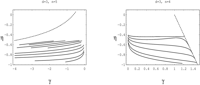
Figure 4: Curves corresponding to $d=3$, $n=5$ ($N=1$, 2, 5, 10, 20, 50, 100, 200, 500, 1000) and $n=4$ ($N=1$, 2, 5, 10, 20, 50).

It is also interesting to compare the curves that correspond to a fixed value for $n$ but for a range of values of $N$. In Fig. 4 we have plotted the case $n=4$ for $d=3$ where the TFP line is also included. We see that the larger the value of $N$ is, the higher the corresponding curve lies. For large values of $N$ they approach the horizontal line $\eta=\eta_{n}$ for $0<\gamma<s_{n}/2$ and the TFP line for $s_{n}/2<\gamma<3/2$. The other plot in Fig. 4 shows the case $n=5$ for $d=3$. Again, larger values of $N$ correspond to higher lying curves. Here we see that the curves tend to the $N=\infty$ horizontal line $\eta=\eta_{5}$ for $\gamma_{*5}<\gamma<0$ and to the $C=0$ curve $\eta=\eta_{1}(\gamma)$ for values $\gamma<\gamma_{*5}$.

4 Conclusions

In this work we have studied the solutions of the leading order Polchinski ERG fixed-point equation for the $O(N)$ scalar field theory. We have described the space of regular solutions corresponding to points of the curves $\eta_{n}(\gamma)$ in the $(\gamma,\eta)$-plane. If for a given $d$ the curve $\eta_{n}$ crosses the $\gamma$-axis at $\gamma=\gamma_{*}$, then the corresponding solution is the physical fixed-point solution with $u_{n}(0;\gamma_{*})=2\gamma_{*}$. We found that the pattern of the curves of regular solutions is universal for any $d$. In this sense each curve represents a fixed-point solution of a certain type.

We have paid special attention to the limit $N=\infty$ where many properties of the space of solutions can be investigated analytically. A general solution is non-analytical at some finite point and, therefore, is not acceptable from the physical point of view. Analyticity imposes a relation between $\eta$ and $\gamma$, thus giving rise to the curves $\eta_{n}(\gamma)$ in the $(\gamma,\eta)$-plane labelled by an integer $n=1,2,\ldots$. For $n\geq 2$ the curves are in fact horizontal straight lines.

For the $N\geq 1$ field theory we also obtained continuous non-trivial fixed-point lines labelled by an integer $n\geq 1$. Clearly, there is a one-to-one correspondence between the lines with equal value of $n$ for $N\geq 1$ and for $N=\infty$. We also found a strong indication that the functions $\eta_{n}(\gamma)$ for finite $N$ transform into the corresponding $N=\infty$ functions $\eta_{n}(\gamma)$ as $N\to\infty$.

References

References

-
[1]
K. Wilson, Rev. Mod. Phys. 47 (1975) 773;
K. Wilson and J. Kogut, Phys. Rep. 12 (1974) 75. - [2] S. Weinberg, in Understanding the Fundamental Constituents of Matter, Erice 1976, edited by A. Zichichi (Plenum, 1978).
- [3] F.J. Wegner and A. Houghton, Phys. Rev. A8 (1973) 401.
- [4] J. Polchinski, Nucl. Phys. B231 (1984) 269.
-
[5]
T.R. Morris, in Zakopane 1997: New Developments in Quantum Field Theory,
edited by P. Damgaard and J. Jurkiewicz (Plenum, 1998) 147, hep-th/9709100;
T.R. Morris, Prog. Theor. Phys. Suppl. 131 (1998) 395. - [6] Y. Kubyshin, Int. J. Mod. Phys. B12 (1998) 1321.
- [7] D.-U. Jungnickel and C. Wetterich, in Proceedings of the Workshop The Exact Renormalization Group, edited by A. Krasnitz, Y. Kubyshin, R. Potting and P. Sá (World Scientific, 1999) 41.
-
[8]
C. Bagnuls and C. Bervillier, Exact
Renormalization Group Equations. An Introductory Review, hep-th/0002034;
J. Berges, N. Tetradis and C. Wetterich, Non-perturbative Renormalization Flow in Quantum Field and Statistical Physics, hep-ph/0005122, to appear in Phys. Rep. - [9] R.D. Ball and R.S. Thorne, Ann. Phys. 236 (1994) 117.
-
[10]
T.R. Morris, Phys. Lett. B329 (1994) 241;
T.R. Morris and J.F. Tighe, JHEP 08 (1999) 007. - [11] R.D. Ball, P.E. Haagensen, J.I. Latorre and E. Moreno, Phys. Lett. B347 (1995) 80.
- [12] Y. Kubyshin, R. Neves and R. Potting, in Proceedings of the Workshop The Exact Renormalization Group, edited by A. Krasnitz, Y. Kubyshin, R. Potting and P. Sá (World Scientific, 1999) 159, hep-th/9811151.
- [13] J. Comellas and A. Travesset, Nucl. Phys. B 498 (1997) 539.
-
[14]
M. Reuter, N. Tetradis and C. Wetterich, Nucl. Phys. B 401 (1993) 567;
M. D’Attanasio and T.R. Morris, Phys. Lett. B409 (1997) 363;
T.R. Morris and M.D. Turner, Nucl. Phys. B 509 (1998) 637. - [15] T.R. Morris, Phys. Lett. B345 (1995) 139.
- [16] Y. Kubyshin, R. Neves and R. Potting, in preparation.