DAMTP-2001-4, HU-EP-01/02, hep-th/0101186

The Dilaton Potential from ${\cal N}=1^{*}$
Anamaría Font^♭, Matthias Klein^♯ and Fernando Quevedo^♯
♭ Humboldt Universität zu Berlin,
Institut für Physik, Invalidenstr. 110, 10115 Berlin, Germany
^♯ DAMTP, Wilberforce Road, Cambridge, CB3 0WA, England.

Recent understanding of ${\cal N}=1^{*}$ supersymmetric theory (mass deformed ${\cal N}=4$) has made it possible to find an exact superpotential which encodes the properties of the different phases of the theory. We consider this superpotential as an illustrative example for the source of a nontrivial scalar potential for the string theory dilaton and study its properties. The superpotential is characterized by the rank of the corresponding gauge group ($N$) and integers $p,q,k$ labelling the different massive phases of the theory. For generic values of these parameters, we find the expected runaway behaviour of the potential to vanishing string coupling. But there are also supersymmetric minima at weak coupling stabilizing the dilaton field. An interesting property of this potential is that there is a proliferation of supersymmetric vacua in the confining phases, with the number of vacua increasing with $N$ and leading to a kind of staircase potential. For a range of parameters, it is possible to obtain realistic values for the gauge coupling.

1 Introduction

The main obstacles for string theory to make contact with low-energy physics have been the breakdown of supersymmetry and the lifting of the large degeneracy of string vacua which manifests itself by the existence of several fields with flat potentials in the low-energy supersymmetric theory: the dilaton and moduli fields. The first problem has been recently reanalysed in the light of low fundamental scale D-brane models in the sense that realistic string models have been obtained with supersymmetry explicitly broken by the presence of anti-D-branes or by D-brane intersections. But besides much progress in understanding supersymmetric string and gauge theories during the past five years, we still have not improved on the outstanding problem of fixing the string theory dilaton and the moduli fields. In perturbative supersymmetric string models the potential for the dilaton and the moduli fields is simply flat. In the recently constructed nonsupersymmetric models (see for instance [1]), even though the flatness of the potential is no longer protected by supersymmetry and the moduli fields may be stabilized, the dilaton is still expected to get a simple runaway behaviour.

The racetrack scenario proposed in the 1980’s [2, 3, 4], based on gaugino condensation for several hidden sector gauge groups, remains as the best option so far for generating a potential for the dilaton field, giving rise to a nontrivial minimum at weak coupling after fine tuning the ranks of the different gauge groups. In this scenario the dilaton field is stabilized at a supersymmetric point and the breaking of supersymmetry is usually achieved by the moduli fields. A detailed study of this scenario was performed in [4], for a recent discussion see [5].

In this note, we will investigate an alternative to the racetrack scenario based on recent developments in understanding ${\cal N}=1$ supersymmetric theories. In particular, we will concentrate on the so-called ${\cal N}=1^{*}$ theory which is obtained from ${\cal N}=4$ super Yang-Mills (SYM) after deforming it by the addition of nonvanishing mass terms for the three adjoint chiral superfields inside the ${\cal N}=4$ vector multiplet. Due to its close relation to ${\cal N}=4$, it has been possible to understand the general phase structure of this theory which has proven to be very rich, including all different phases that ’t Hooft predicted for a general class of gauge theories in the past. A general superpotential that describes the different phases of the theory and transforms in a well defined way under the $SL(2,{\mathbb{Z}})$ of the original ${\cal N}=4$ theory was found in [6]. It was shown to be the exact superpotential of the effective low-energy description where all massive degrees of freedom are integrated out. Furthermore, in [7] a very detailed analysis of this theory provided nontrivial evidence for the extension of the AdS/CFT correspondence to the ${\cal N}=1$ case and uncovered the detailed brane realization of the different confining and Higgs phases. The nonsingular supergravity dual allows for physical quantities, such as different condensates, to be calculable. The explicit form of the superpotential of [6], which includes an infinite sum over instantons and fractional instantons, also provides successful comparisons between the string and field theory pictures [8].

Using the information we have about this special ${\cal N}=1$ theory, and in particular the expression for the exact superpotential for each massive phase, $W(\tau)$ with $\tau=\theta/2\pi+i4\pi/g^{2}$, we may immediately think about the possibility that $\tau$ could actually be promoted to a field as it happens in string theory, where, at tree-level, it corresponds to the dilaton field. This may happen if the ${\cal N}=1^{*}$ theory could be part of a string hidden sector and therefore the corresponding superpotential can be seen as a dynamically generated superpotential for the dilaton field. The most natural realization of this idea is the world-volume gauge theory on a set of D3-branes in type IIB string theory. However, one may also imagine some heterotic string vacuum having an ${\cal N}=1^{*}$ subsector. Of course, this approach is only self-consistent if the masses of the adjoint fields of the ${\cal N}=1^{*}$ theory are by at least one order of magnitude smaller than the string scale. Else one would have to take into account the massive string states as well and would therefore loose the justification to study the ${\cal N}=1^{*}$ theory. Throughout this article, we assume that such a self-consistent mass-deformation of ${\cal N}=4$ SYM does exist. At the end of section 3, we suggest a way how to realize this assumption in a concrete model. However, in this paper we do not attempt to present a full model. Our work rather seeks to explore the consequences of recently studied non-perturbative ${\cal N}=1$ dynamics for the dilaton behavior. Indeed, in this note we study the dilaton potential of ${\cal N}=1^{*}$. More precisely, we analyse the scalar potential of the supergravity Lagrangian derived from the superpotential for $\tau$. The main result is that there are minima that stabilize $\tau$ at weak coupling.

2 Generalities

We will start by briefly recalling the status of the dilaton potential in string theory. Let us, for simplicity, concentrate only on the dilaton field. In compactified ${\cal N}=1$ supersymmetric models, after a duality transformation this field corresponds to $S=(2\,R_{1}R_{2}R_{3}/(\alpha^{\prime})^{3})e^{-\phi}+ia$, where $R_{i}$ are the compactification radii, $\phi$ is the original 10D dilaton field and the axion field $a$ is dual to the original $B_{\mu\nu}$ field. Both $\phi$ and $B_{\mu\nu}$ appear in all string theories, and the scalar potential for $S$ vanishes to all orders in perturbation theory.

Since the early days of string theory, the stabilization of the dilaton field has been considered one of the major obstacles preventing string models from making contact with low-energy physics. Dine and Seiberg [9] gave a very general argument in which, whatever the source of the potential for $S$ is, it has to be such that it runs away to $S\to\infty$. Then, they argued, if there is any other minimum at finite $S$ it has to be at strong coupling, since $S+S^{*}\sim 1/g^{2}$, and therefore, unless there is a ‘natural’ fine tuning at work, it is not achievable in weak coupling strings.

Over the years there have been several proposals for generating a potential for the dilaton field [2, 3, 10, 11, 12, 13, 14, 15, 16]. The most successful so far has been the racetrack scenario where it is assumed that the hidden sector of string theory has a product group structure. Gaugino condensation for each group factor is expected to generate superpotentials of the form $W_{i}=\exp(-6\pi S/b_{i})$, with $b_{i}$ being the one-loop beta function coefficients of the corresponding gauge theory. Each $W_{i}$ has a clear runaway behaviour but summing the different superpotentials $W=\sum{\alpha_{i}W_{i}}$ gives rise to a scalar potential that may have a nontrivial minimum, stabilizing the dilaton. For a hidden group of the form $SU(N_{1})\times SU(N_{2})$, the minimum in global supersymmetry occurs at

$$2\pi\,S=\frac{N_{1}N_{2}}{N_{1}-N_{2}}\ \log\left(-\frac{\alpha_{2}N_{1}}{\alpha_{1}N_{2}}\right).$$ (2.1)

The ranks $N_{1},N_{2}$ may be (discretely) fine tuned to get a realistic value for $S$. It may be seen on general grounds [17, 4] that in both global and local supersymmetry, the minimum of the potential for $S$ is such that supersymmetry is not broken. Then the breaking of supersymmetry is left to the other fields in the theory, such as the moduli fields [18]. Even with the natural problems of this scenario, regarding especially the fine tuning plus other possible cosmological ones [19, 20], this is at the moment the best proposal we have for stabilizing the dilaton.

Another proposal that was put forward was the use of $S$-duality. Assuming that there are self-dual ${\cal N}=1$ models, the possible induced superpotentials should transform in a definite way under the conjectured $SL(2,{\mathbb{Z}})$ transformations and several functional forms have been considered [10, 11]. This proposal has several problems: first, the fact that the superpotential has to be a modular form of negative weight implies the existence of poles in the fundamental domain. If the poles are at $S\to\infty$ [10], then we do not recover the weak coupling behaviour expected from the general Dine-Seiberg arguments. Otherwise [11] there are singularities at finite values of the string coupling without a clear physical interpretation. Second, since the self-dual points $S=1,e^{i\pi/6}$ are necessarily extrema of the invariant potential, then the natural value for $S$ is of order $S\sim 1$ which means strong coupling. Finally there are no explicit models which are self-dual under $S$-duality that can provide the superpotentials used in [10, 11].

Most of the work done in the past was based on the heterotic string but, the dilaton being universal, the situation is similar for other string theories. However, it is worth pointing out the differences. First, in type I and type II compactifications, the fundamental scale may be substantially lower than the Planck scale [21]. Therefore the difference between the supersymmetry breaking scale $\Lambda$ and the string scale does not have to be very large in order to have a realistic supersymmetry breaking at low energies. Second, the expression for the gauge couplings may differ from just being $f=S$ at tree level. It has been found in orientifold models that the gauge couplings at tree level depend not only on $S$ but also on the blowing-up modes $M$: $f=S+kM$ and, depending on the dimension of the brane that hosts the gauge group, the gauge coupling may not depend on $S$ at all but take the form $f=T+kM$ [22]. The effective action after gaugino condensation will then be much richer than in the pure heterotic case because of this dependence [15, 16]. Also since these models are not self-dual under $T$-duality, the threshold corrections to the gauge coupling differ from those of the heterotic string. Finally, because the fundamental scale may be much lower than the Planck scale, there exist now quasi-realistic string models which are already nonsupersymmetric, which in principle can lift the flat directions. This is expected for the moduli fields since there may be a particular radius which minimizes the energy (see the fourth paper of reference [1] for a concrete potential). But since these are weak coupling vacua, the dilaton potential is just the runaway and nonperturbative effects may still be needed to stabilize the dilaton. A complete analysis of all of these situations is beyond the scope of this note and we will only concentrate on the particular case $f=S$.

3 The ${\cal N}=1^{*}$ Theory

Let us review the main aspects of the ${\cal N}=1^{*}$ theory. The starting point is ${\cal N}=4$, $SU(N)$ super Yang-Mills, which in terms of ${\cal N}=1$ is a gauge theory with three massless adjoint chiral multiplets $\Phi_{i}$ and superpotential

$$W\ =\ \epsilon_{ijk}\,{\rm Tr\,}{\Phi_{i}[\Phi_{j},\Phi_{k}]}.$$ (3.1)

Deforming this theory by nonzero mass terms for the fields $\Phi_{i}$,

$$\Delta W\ =\ m_{1}\,{\rm Tr\,}\Phi_{1}^{2}+\ m_{2}\,{\rm Tr\,}\Phi_{2}^{2}\ +m_{3}\,{\rm Tr\,}\Phi_{3}^{2},$$ (3.2)

breaks supersymmetry to ${\cal N}=1$ (unless $m_{1}=0,m_{2}=m_{3}$ which gives ${\cal N}=2$). The generic case where none of the masses vanishes is called ${\cal N}=1^{*}$ [6, 7, 8].

The classical vacua of this theory can be found by solving $\partial W/\partial\Phi_{i}\ =\ 0$, which leads to

$$[\Phi_{i},\Phi_{j}]=\epsilon_{ijk}\,m_{k}\,\Phi_{k}.$$ (3.3)

Therefore the fields $\Phi_{i}$ are $N$-dimensional representations of the $SU(2)$ algebra and there is a vacuum for each representation. Since there is one irreducible representation $SU(2)$ for every dimension $d$ ($d=2j+1$), the number of vacua is determined by the number of partitions of $N$. The irreducible $d=N$ representation breaks the $SU(N)$ symmetry completely and it is identified then with the Higgs phase. The identity representation ($\langle\Phi_{i}\rangle=0$) leaves the full gauge group unbroken, corresponding to the confining phase of the theory.

All other $N$-dimensional reducible representations represent intermediate cases. For instance, if we have a product of two irreps of dimension $p_{1}$ and $p_{2}$ (with $p_{1}+p_{2}=N$), the generator $-p_{2}{\rm 1\kern-2.59995ptI}_{p_{1}}\oplus p_{1}{\rm 1\kern-2.59995ptI}_{p_{2}}$ is left invariant, generating a $U(1)$ symmetry. If there are $l$ of these blocks, there will be a remaining $U(1)^{l-1}$ symmetry left. These then correspond to the Coulomb phases of the theory. However, if above we have $p_{1}=p_{2}=N/2$, there will be two extra off-diagonal generators left invariant promoting the symmetry to $SU(2)$ and in the general case of $q$ blocks of dimension $p$ with $pq=N$, this generalizes to a nonabelian $SU(q)$ symmetry left invariant. These are the confining phases of the corresponding $SU(q)$ remnant theory which will have a mass gap and can then be called the massive phases to differentiate them from the Coulomb phases which have no gap. The massive phases are then labelled by the two integers $p,q$ (with the original confining phase corresponding to $q=N$). Since $pq=N$, the phases are determined by the divisors of $N$. Furthermore, Donagi and Witten [23] found that the quantum vacua are such that for each $q$, the $SU(q)$ theory in turn splits into $q$ different vacua labelled by an integer $k=0,\cdots,q-1$. These $q$ vacua, unlike the case of pure super Yang-Mills, are not equivalent. Therefore we label the massive phases as $(p,q,k)$.

The massive phase structure of the ${\cal N}=1^{*}$ theory has been shown [23] to be rich enough as to realize all the different phases of a class of gauge theories classified by ’t Hooft in the past [24]. He found that the vacua of an $SU(N)$ gauge theory in which all fields transform trivially under the centre of $SU(N)$ are in one-to-one correspondence with the order-$N$ subgroups of ${\mathbb{Z}}_{N}\times{\mathbb{Z}}_{N}$. Using the integer parameters $p,q,k$, introduced above, this correspondence can be made precise in the ${\cal N}=1^{*}$ theory [23]: The phase labelled by $(p,q,k)$ is associated with the ${\mathbb{Z}}_{N}\times{\mathbb{Z}}_{N}$ subgroup generated by $(p,k)$ and $(0,q)$. The $SL(2,{\mathbb{Z}})$ $S$-duality of the original ${\cal N}=4$ theory, $\tau\rightarrow(a\tau+b)/(c\tau+d)$, $ad-bc=1$, is no longer a symmetry of the ${\cal N}=1^{*}$ theory but still acts in a very interesting way on these phases, permuting the phases among themselves. Under an $SL(2,{\mathbb{Z}})$ transformation, the phase $(p,q,k)$ is mapped to the phase $(p^{\prime},q^{\prime},k^{\prime})$, where $(p^{\prime},k^{\prime})$, $(0,q^{\prime})$ are the (standard) generators of the order-$N$ subgroup that is also generated by

$$\left(\tilde{k}\atop\tilde{p}\right)=\left(\begin{array}[]{cc}a&b\\ c&d\end{array}\right)\left(k\atop p\right),\qquad\left(\tilde{q}\atop\tilde{r}\right)=\left(\begin{array}[]{cc}a&b\\ c&d\end{array}\right)\left(q\atop 0\right).$$ (3.4)

It is straightforward to show that this implies

$$\tau\to\tau+1 \quad{\rm maps}\quad (p,q,k)\to(p,q,k+p),$$

$$\tau\to-{1\over\tau} \quad{\rm maps}\quad (p,q,k)\to(\alpha,{N\over\alpha},k^{\prime}),$$

$${\rm with}\ \alpha=gcd(k,q).$$

In general, the dependence of $k^{\prime}$ on $p,q,k$ is complicated, but there are two simple special cases: $k^{\prime}=0$ if $k=0$ and $k^{\prime}=N-p$ if $k=1$. The first statement implies that the transformation $\tau\to-1/\tau$ exchanges Higgs and confinement phases.

In [6] an exact superpotential was derived for this theory by using instanton techniques for the theory compactified on a circle. The compactification to three dimensions is a computational trick and it turns out that the superpotential is independent of the compactification radius. After integrating out the gauge fields, it takes the form:

$$W_{p,q,k}(\tau)=E_{2}(\tau)-\frac{p}{q}\ E_{2}\left(\frac{p}{q}\tau+\frac{k}{q}\right)$$ (3.6)

Here $E_{2}$ is the holomorphic second Eisenstein series:

$$E_{2}(\tau)\ =\ {3\over\pi^{2}}\ \sum_{n=-\infty}^{\infty}\ \sum_{m=-\infty}^{\infty}\ \frac{1}{(m+n\tau)^{2}},$$ (3.7)

where the sum excludes the term $m=n=0$. As it is clear, each phase of the theory has a different superpotential and even though each $E_{2}$ series in (3.6) does not transform covariantly under $SL(2,{\mathbb{Z}})$ modular transformations, their difference is a modular form of weight two up to some permutation of the phases. Notice that $SL(2,{\mathbb{Z}})$ is $not$ a symmetry of the theory but it maps different phases to one another. The superpotential reflects the $SL(2,{\mathbb{Z}})$ properties of the theory in an interesting way. For instance, it is clear that under $\tau\rightarrow\tau+1$, $W_{p,q,k}\to W_{p,q,k+p}$ and, more generally, one can show that

$$W_{p,q,k}\left({a\tau+b\over c\tau+d}\right)=(c\tau+d)^{2}W_{p^{\prime},q^{\prime},k^{\prime}}(\tau),$$ (3.8)

where $p^{\prime},q^{\prime},k^{\prime}$ are determined as explained in the paragraph before eq. (3.4).

Before discussing the minimization of the scalar potential in detail in the following section, we would like to give a qualitative argument why we expect the scalar potential to have a minimum at large values of $\tau$. The Eisenstein series has a rich structure at values of its argument of order $1/2\pi$ and it drops exponentially to a constant for large values of its argument. Thus, for $p\ll q$, the first $E_{2}$ in (3.6) can be approximated by a constant and the second $E_{2}$ has a rich structure at $\tau\gg 1/2\pi$. Besides the constant term in the expansion, $W$ then looks like an infinite sum of gaugino condensates.

To finish this section, let us address the following issue: as mentioned in the introduction we are assuming that the masses of the adjoint scalar fields are smaller than the string scale in order to be able to consider the ${\cal N}=1^{*}$ as an effective field theory below the string scale. Let us then comment on how the ${\cal N}=1^{*}$ theory appears in string theory and why the masses of the adjoint fields do not necessarily have to be of the order of the string scale. The most natural realization is on a set of $N$ D3-branes. We think of these D3-branes as filling the 3+1 space-time dimensions and being located at a nonsingular point of some 6-dimensional compact space. The theory living on the D3-branes is an ${\cal N}=4$ $U(N)$ gauge theory. We know of two ways to switch on a mass deformation that breaks the supersymmetry down to ${\cal N}=1$.

First, we will consider the ${\cal N}=1^{*}$ theory as it arises in the context of the AdS/CFT correspondence. As discovered by Myers [25], D$p$-branes can couple to $(p+3)$-form RR potentials. In particular, consider $N$ D0-branes in flat space. The equations of motion of the 9 adjoint fields $\phi_{i}$, $i=1,\ldots,9$, whose expectation values parametrise the positions of the D0-branes are $[\phi_{i},\phi_{j}]=0$ $\forall\,i,j$. All the $\phi_{i}$ can be simultaneously diagonalized and the $N$ eigenvalues of $\langle\phi_{i}\rangle$ are interpreted as the $i^{\rm th}$ coordinate of the positions of the D0-branes. Turning on a background flux of the RR 4-form field strength

$$F^{(4)}_{0ijk}=\left\{\begin{array}[]{ll}-2\,m\,\epsilon_{ijk}&{\rm if}\ i,j,k\in\{1,2,3\}\\ 0&{\rm else}\end{array}\right.$$ (3.9)

changes the scalar potential of the gauge theory on the D0 world-line and leads to the modified equations of motion [25]

$$[\phi^{i},\phi^{j}]=im\,\epsilon_{ijk}\,\phi^{k},\quad{\rm for}\ i,j,k\in\{1,2,3\}.$$ (3.10)

The geometry of this configuration is noncommutative. It describes a fuzzy 2-sphere of radius

$$R=\left(\sum_{i=1}^{3}\frac{1}{N}{\rm Tr\,}(\phi_{i}^{2})\right)=\frac{m}{2}N\sqrt{1-\frac{1}{N^{2}}}.$$ (3.11)

The equations of motion (3.10) of the adjoint fields $\phi_{1}$, $\phi_{2}$, $\phi_{3}$ living on the D0 world-line remind us the equations of motion (3.3) of the adjoint fields of ${\cal N}=1^{*}$. Indeed, Polchinski and Strassler [7] showed that the Myers effect applied to D3-branes in AdS${}_{5}\times S^{5}$ space-time leads to the expected mass deformation (3.2) for the adjoint fields of the ${\cal N}=4$ SYM. More precisely, switching on a background flux of the RR 7-form field strength of the form $F^{(7)}_{0123ijk}=\alpha\,m_{k}\,\epsilon_{ijk}$ if $i,j,k\in\{4,5,6\}$ implies (3.3) for the adjoint fields phase rotated to their real parts. Here, $\alpha$ contains some numerical factors due to the AdS${}_{5}\times S^{5}$ space-time. At this level, the RR 7-form is an arbitrary parameter which can be chosen such that the masses are significantly smaller than the string scale. Therefore the RR flux can be seen as providing an independent scale from the string scale in much the same way as the compactification scale does not have to be the same as the string scale.

Second, one can foresee the following scenario: take the compact six dimensions to form an orbifold space that preserves ${\cal N}=1$ supersymmetry. Putting $N$ D3-branes in the bulk, i.e., at some nonsingular point of the orbifold, results in an ${\cal N}=4$ SYM on their world-volume. Let us denote by $A$ this set of D-branes and put another set — denoted $B$ — at a singular point of the orbifold. The gauge theory on the latter will only be ${\cal N}=1$ supersymmetric due to the orbifold action. The two sectors of the model only interact gravitationally. As a consequence, the partial supersymmetry breaking from ${\cal N}=4$ to ${\cal N}=1$ in the $B$-sector will be transmitted to the $A$-sector via gravitational interactions. This will give masses to the adjoint chiral superfields $\Phi_{i}$. Using dimensional analysis, the size of the masses can be estimated to be of the order $m\sim M_{\rm str}^{2}/M_{\rm Pl}$, where we used that supersymmetry is partially broken at the string scale in the $B$-sector. Thus, for low or intermediate string scale, the masses of the adjoint fields may be naturally suppressed with respect to the string scale. As we mentioned in the introduction, the explicit construction of string models with these characteristics is beyond the scope of the present work.

4 The Dilaton Potential

We will now promote the parameter $\tau$ to a full ${\cal N}=1$ superfield that as mentioned before may be several combinations of the dilaton and other moduli fields in different string theories. In this note we focus on the dilaton and set $S=-i\tau=(2\,R_{1}R_{2}R_{3}/(\alpha^{\prime})^{3})e^{-\phi}+ia$. We consider the superpotential

$$W_{p,q,k}(S)=E_{2}(S)-\mu E_{2}(\tilde{S}),$$ (4.1)

where $\tilde{S}=\mu S-i\nu$, $\mu=p/q$ and $\nu=k/q$. In the following we will usually drop the sub-indices in $W$. We will mostly work with the $E_{2}(S)$ expansions in terms of the variable $\exp(-2\pi\,S)$ that are given in the appendix. Clearly $W(S)$ is periodic in ${\rm Im}\,S$ with a period that depends on the particular values of $p,q$. Notice that $W$ goes to the constant $(1-\mu)$ for large $S$. On the other hand, $W$ diverges as $1/S^{2}$ for small $S$, as found using (6.3).

Our purpose is to study the scalar potential $V(S)$ which also depends on the Kähler potential that determines the dilaton kinetic energy. We take the weak coupling result in 4-dimensional string models, namely

$$K=-\log(S+S^{*}),$$ (4.2)

and neglect possible perturbative and nonperturbative corrections.

Let us first discuss the case of global supersymmetry in which

$$V=K^{-1}_{SS^{*}}|W_{S}|^{2}=(S+S^{*})^{2}|W_{S}|^{2}$$ (4.3)

Using the formulae provided in the appendix we find

$$W_{S}=\frac{\pi}{6}\left\{[E_{4}(S)-E_{2}^{2}(S)]-\mu^{2}[E_{4}(\tilde{S})-E_{2}^{2}(\tilde{S})]\right\}.$$ (4.4)

For large $S$, $W_{S}$ tends to zero as $\exp(-2\pi\,S)$, whereas for small $S$ it diverges as $1/S^{3}$. Hence, $V$ diverges at small $S$ and vanishes at large $S$. Our numerical analysis indicates that in between $V$ has a minimum and its behaviour in the ${\rm Re}\,S$ direction is of the form shown in figure 1. At the minimum supersymmetry is not broken since $\langle W_{S}\rangle=0$. For the class of models with $p=1$ and $q=N$ we find that the supersymmetric minimum is located at

$${\rm Im}\,S=\frac{N}{2}+k,\quad\quad\quad\quad{\rm Re}\,S\approx 0.24104\,N,$$ (4.5)

which corresponds to weak coupling for $N\geq 5$. This result can be derived semi-analytically by noticing that for large $S$ the second term in $W$ dominates. Therefore the supersymmetric minimum is to very good approximation located at values $S_{\rm min}$ that satisfy $E_{2}^{\prime}({S_{\rm min}-ik\over N})=0$, where the prime denotes derivative. The numerical analysis leads us to believe that there is only one minimum (up to the periodicity $S\to S+iN$), but we were not able to prove this.

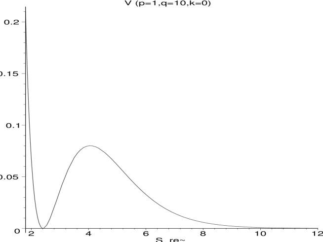
Figure 1: Dilaton potential in global supersymmetry.

Let us now turn to the case of local supersymmetry. The scalar potential and its first derivative turn out to be

$$V = \frac{1}{S_{R}}\left\{|S_{R}W_{S}-W|^{2}-3|W|^{2}\right\},$$

$$\frac{\partial V}{\partial S} = W_{SS}(S_{R}W_{S}-W)^{*}-\frac{2W^{*}}{S_{R}^{2}}(S_{R}W_{S}-W),$$ (4.6)

where $S_{R}=S+S^{*}$. Notice then that there can be two types of extrema. The supersymmetric extrema appear when

$$S_{R}W_{S}-W=0.$$ (4.7)

These extrema are minima provided that $S_{R}^{2}|W_{SS}|>2|W|$. The nonsupersymmetric extrema occur at

$$S_{R}^{2}W_{SS}=2W^{*}e^{2i\gamma},$$ (4.8)

where $\gamma=\arg(S_{R}W_{S}-W)$. As discussed below, our numerical analysis indicates that all minima satisfy (4.7) so that they are supersymmetric and lead to negative cosmological constant.

We have explored to some detail the class of models with $p=1$ and $q=N$ for which it is enough to set $k=0$ since $k\not=0$ can be reached by a translation $S\to S-ik$. In order to perform reliable computations with the Eisenstein series we use the weak coupling expansion of $W(S)$ in eq. (4.1) only when $2\pi\,{\rm Re}\,S>N$. For other ranges we can use the property (6.3). For instance, for $1<2\pi\,{\rm Re}\,S<N$ we can transform the $E_{2}(\frac{S}{N})$ term to obtain

$$W(S)=E_{2}(S)+\frac{N}{S^{2}}E_{2}(\frac{N}{S})-\frac{6}{\pi S}.$$ (4.9)

Similarly, when $2\pi\,{\rm Re}\,S<1$ we can transform both terms in $W(S)$ to obtain

$$W(S)=-\frac{1}{S^{2}}E_{2}(S)+\frac{N}{S^{2}}E_{2}(\frac{N}{S}).$$ (4.10)

For $N\leq 8$ we find one supersymmetric minimum at ${\rm Im}\,S=\frac{N}{2}$ and ${\rm Re}\,S$ given in table 1.

$N$	2	3	4	5	6	7	8
${\rm Re}\,S$	1.81	2.29	2.70	3.04	3.30	3.45	3.37

Table 1: Minima of the scalar potential.

For $N\geq 9$ this minimum turns into a saddle point and two supersymmetric minima $S_{11}$, $S_{12}$ on either side in the ${\rm Im}\,S$ direction appear, such that ${\rm Im}\,S_{12}+{\rm Im}\,S_{11}=N$ and ${\rm Re}\,S_{12}={\rm Re}\,S_{11}$. Examples are given in tables 2, 3.

$N$	10	20	30	40	50	60	70	80	90	100
${\rm Re}\,S_{11}$	3.08	3.95	4.50	4.92	5.30	5.65	5.96	6.26	6.53	6.79
${\rm Im}\,S_{11}$	4.07	6.11	7.49	8.66	9.69	10.61	11.45	12.23	12.97	13.66

Table 2: Minima of the scalar potential.

$N$	200	300	400	500	600	700	800	900	1000	2000
${\rm Re}\,S_{11}$	8.89	10.49	11.84	13.03	14.09	15.09	16.01	16.86	17.67	24.23
${\rm Im}\,S_{11}$	19.21	23.45	27.02	30.16	32.99	35.60	38.05	40.30	42.45	59.81

Table 3: Minima of the scalar potential.

For large $N$ (say $N\geq 20$) these results agree well with those obtained using for $W$ the approximation

$$W\sim 1+\frac{N}{S^{2}}-\frac{6}{\pi S}.$$ (4.11)

This approximation is derived from (4.9) by keeping only the constant terms in the $E_{2}$ expansions. It is valid when $(2\pi\,{\rm Re}\,S)\,N\gg({\rm Re}\,S)^{2}+({\rm Im}\,S)^{2}$.

Now, as $N$ grows, there appear more supersymmetric minima, always in pairs $S_{i1}$, $S_{i2}$ with ${\rm Im}\,S_{i2}+{\rm Im}\,S_{i1}=N$ and ${\rm Re}\,S_{i2}={\rm Re}\,S_{i1}$, $i=1,\cdots,n$. We have not performed an extensive numerical analysis and thus limit ourselves to pointing some observations. The number $n$ of minima grows with $N$. For instance, we found $n=8$ for $N=100$, although we cannot exclude that there exist even more minima. It turns out that the absolute minimum is among the new minima that have ${\rm Im}\,S_{i1}\geq{\rm Im}\,S_{11}$ and ${\rm Re}\,S_{i1}\leq{\rm Re}\,S_{11}$. We label by $S_{n1}$ the minimum with the lowest value of the potential that we found. In table  4 we give the values of these minima in various cases.

$N$	20	30	40	50	60	70	80	90	100
${\rm Re}\,S_{n1}$	2.38	3.05	2.41	2.76	3.04	2.49	2.69	2.88	3.04
${\rm Im}\,S_{n1}$	7.46	11.66	11.07	13.99	16.91	15.29	17.54	19.80	22.05

Table 4: Further Minima of the scalar potential.

Using the approximate superpotential in (4.11), the condition for a susy minimum, i.e., $D_{S}W=0$, reduces to a cubic equation which can be solved analytically. The general solution is very complicated and not illuminating but there is a nice expansion in powers of $\sqrt{N}$. One has

$$2\pi\,{\rm Re}\,S_{\rm min}=\sum_{n=1}^{\infty}c_{n}\left(\pi\sqrt{N}\right)^{2-n},$$ (4.12)

where the first coefficients are $c_{1}=1,c_{2}=12,c_{3}=-36,c_{4}=648$. Moreover we found a recursion formula for the $c_{n}$. Given $c_{1}$ and $c_{2}$, they can be obtained from

$$c_{r}=-\frac{1}{2}\sum_{\scriptstyle n+m+k=r+2\atop\scriptstyle n,m,k<r}\!\!\!\!\!\!c_{n}c_{m}c_{k}+9\sum_{n+m=r}\!\!c_{n}c_{m}-36\,c_{r-2}.$$ (4.13)

The solution for the imaginary part of $S$ is similar:

$$2\pi\,{\rm Im}\,S=\frac{1}{\sqrt{7}}\ \sum_{n=1}^{\infty}d_{n}(7\pi\sqrt{N})^{2-n},$$ (4.14)

with $d_{1}=1,d_{2}=12,d_{3}=-1332,d_{4}=90072,\ldots$

If one neglects the term $6/(\pi S)$ in (4.11), the condition for a susy minimum reduces to a quadratic equation with a very simple solution: ${\rm Re}\,S=1/2\sqrt{N},\ {\rm Im}\,S=1/2\sqrt{7N}$. This is just the first term in the above expansions, but the approximation is rather rough. The series converges very slowly. But in general it will give us an idea for the values of $N$ required to get ‘realistic’ gauge couplings. In the standard unification picture we need ${\rm Re}\,S\sim 20$ indicating that a very large value of $N$ may be needed. This is not possible to get in perturbative heterotic strings but in more general vacua including $F$-theory and orientifold models this is easily achievable [26]. We present in the figures examples of the general behaviour of the potentials regarding periodicity, runaway to infinity and supersymmetric minima at weak coupling. We explicitly show the case $q=N=1000$ for different ranges of values of Re$\,S$ and Im$\,S$ around the supersymmetric weak coupling minimum.

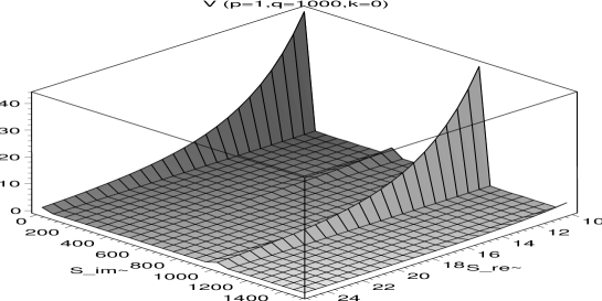
Figure 2: Case $q=N=1000$: Periodicity of the potential.

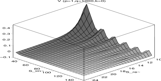
Figure 3: Case $q=N=1000$: Structure of the potential.

Figure 4: Case $q=N=1000$: Minimum of the potential.

The case $p=N$, $q=1$ is easily derived from the above. Indeed, notice that $W_{N,1,0}(S)=-N\,W_{1,N,0}(NS)$ and hence the minima will be those found previously divided by $N$. We have also considered a few examples with $N\not=p\not=1$ and found similar results. For example, for $p=2$, $q=4$, there is a supersymmetric minimum at ${\rm Re}\,S=1.8103$ and ${\rm Im}\,S=1$, whereas for for $p=2$, $q=5$, there are two supersymmetric minima at ${\rm Re}\,S_{1}={\rm Re}\,S_{2}=2.0562$ and ${\rm Im}\,S_{1}=5-{\rm Im}\,S_{2}=1.2489$. Finally the, case $p=q$ and $k\not=0$ has also supersymmetric minima that generally occur at small ${\rm Re}\,S$ and lead to larger values of the cosmological constant.

Regarding nonsupersymmetric extrema, all the ones we have found correspond to maxima or saddle points. So it seems that all the vacua of this theory are supersymmetric, but we still lack a proof that this is the general situation.

5 Discussion

We have seen that the nonperturbative dilaton potential for ${\cal N}=1^{*}$ theory has very interesting properties. In particular, it can stabilize the dilaton field at weak string coupling in a natural way. The discrete fine tuning required to overcome the Dine-Seiberg problem is naturally provided in the theory by the integers $p,q,k$ determining the phases. We have seen that the minima we found generically do not break supersymmetry, which is similar to the situation of the racetrack scenario. This situation may change once corrections to the Kähler potential are included, perturbative and nonperturbative. Furthermore, once the other moduli fields $T$ are included, they tend to break supersymmetry. Our results for the minima in the $S$ direction will be preserved whenever the superpotential is a product $W(S,T)=\Omega(S)\Gamma(T)$ and the Kähler potential does not have a large $S-T$ mixing. This is certainly the case in perturbative heterotic strings where $\Gamma(T)$ comes from threshold corrections to the gauge coupling constant. In the simplest case of constant $\Gamma(T)$ we have a realization of the no-scale scenario with supersymmetry broken and vanishing cosmological constant and $T$ arbitrary. More generally, $T$ will be fixed with a negative cosmological constant [18].

Notice that the situation we have has some similarities with the racetrack scenario, although perhaps improving on the discrete fine tuning part. It shares some of the positive properties, such as the overcoming of Dine-Seiberg problem and fixing the dilaton without breaking supersymmetry. It may also share some of the problems. In particular, the cosmological constant does not have to be small at the minimum after supersymmetry is broken. Furthermore the cosmological problems emphasized in [19]  about the dilaton field overrunning the nontrivial minimum towards the runaway one for generic initial conditions, may still hold in this case as well as the proposed ameliorations [27], similarly for the cosmological moduli problem [20].

There are also some significant differences, besides the theoretical one of having an underlying $SL(2,{\mathbb{Z}})$ symmetry mapping the different massive phases. In particular the constant term in the superpotential is not present in the many condensates case. It is actually more reminiscent of the original stringy gaugino condensation discussions with a constant term added from the antisymmetric tensor field [2]. The presence of this constant term has at least one important impact: after supersymmetry is broken, the scale of supersymmetry breaking is not exponentially supressed as compared to the string scale as in gaugino condensation models where $M_{SUSY}=M_{String}e^{-b/g^{2}}$. In our case it will depend on how supersymmetry is broken. But if the scale is proportional to the superpotential, the constant term will dominate over the exponentially suppressed ones and both scales will be similar. This may be consistent with a low or intermediate scale for string theory [21, 28].

Probably the clearest difference from previous proposals is the large proliferation of supersymmetric vacua at large $N$ on top of the standard repetition of minima from the periodicity of the potential. This may have some interesting consequences, especially regarding cosmology. The many vacua structure is such that we have a realization of a staircase potential, once we project on some line in the Re$\,S$ / Im$\,S$ plane, with the staircase climbing towards the zero coupling vacuum. Each vacuum has different (negative) energy but all of them are stable according to the general analysis of Coleman-de Luccia [29]. We can imagine then many different regions of the universe living on different vacua with static BPS domain wall boundaries. The critical tension of the domain walls is determined by the difference of the value of the superpotentials for the corresponding minima [30]. In general, the vacua are stable if the tension of the wall is bounded by the BPS condition, but the walls are not static if the BPS condition is not satisfied. The general properties of these domain walls have been investigated thoroughly (see [31] for a review on domain walls in supergravity theories). For some interesting recent ideas along these lines see [32].

Once, more fields are considered, the physical implications of the proliferation of vacua changes. In the simple no-scale models for instance, all the vacua would be degenerate with vanishing cosmological constant and broken supersymmetry. We may even foresee that the addition of other fields and corrections to the Kähler potential may revert the staircase behaviour producing a potential similar to the one proposed by Abbott [33] trying to ameliorate the cosmological constant problem (this may happen for instance if there is a field $U$ not entering in the superpotential with Kähler potential $K=-n\log(U+U^{*})$ and $n>3$, although we do not see how this situation may be realized in string theory).

An interesting open question would be to find an explicit realization of the present scenario in a concrete string model by looking for hidden sectors, perhaps on a set of hidden D3-branes corresponding to ${\cal N}=1^{*}$. One might hope however that since the massive phase structure of the ${\cal N}=1^{*}$ theory is very rich and realizes all the phases predicted by ’t Hooft, the results we have found in this note may also apply to more general ${\cal N}=1$ theories.

Acknowledgements

We thank Ralph Blumenhagen, Cliff Burgess, Elena Cáceres, Massimo Bianchi, Nick Dorey, Michael Green, Luis Ibáñez, Stefano Kovacs, Prem Kumar, Dieter Lüst, Graham Ross and Radu Tatar for useful conversations. This research is partially funded by PPARC. A.F. acknowledges a fellowship from the Alexander von Humboldt Foundation.

6 Appendix

In this appendix we collect some definitions and useful properties.

The Eisenstein modular functions that enter in the scalar potential and its derivatives are

$$E_{2} = 1-24\sum_{n=1}^{\infty}\sigma_{1}(n)q^{n},$$

$$E_{4} = 1+240\sum_{n=1}^{\infty}\sigma_{3}(n)q^{n},$$

$$E_{6} = 1-504\sum_{n=1}^{\infty}\sigma_{5}(n)q^{n},$$ (6.1)

where $q=e^{-2\pi\,S}$ and $\sigma_{p}(n)$ is the sum of the $p^{\rm th}$ powers of all divisors of $n$. $E_{4}$ and $E_{6}$ are modular forms of weight 4 and 6 respectively. This means

$$E_{4}\left(\frac{1}{S}\right)=S^{4}E_{4}(S),\quad\quad\quad\quad E_{6}\left(\frac{1}{S}\right)=-S^{6}E_{6}(S).$$ (6.2)

$E_{4}(S)$ has a zero at $S=e^{i\pi/6}$ and $E_{6}(S)$ at $S=1$. $E_{2}$ fails to be a modular form of weight two since

$$E_{2}\left(\frac{1}{S}\right)=-S^{2}E_{2}(S)+\frac{6S}{\pi}.$$ (6.3)

It is useful to introduce

$$\hat{E}_{2}(S)=E_{2}(S)-\frac{6}{\pi(S+S^{*})},\quad\quad\quad\quad\hat{E}_{2}\left(\frac{1}{S}\right)=-S^{2}\hat{E}_{2}(S).$$ (6.4)

$\hat{E}_{2}(S)$ has zeroes at $S=1,e^{i\pi/6}$.

We also have the following derivatives

$$E_{4}^{\prime} = \frac{2\pi}{3}(E_{6}-E_{2}E_{4}),$$

$$E_{2}^{\prime} = \frac{\pi}{6}(E_{4}-E_{2}^{2}),$$

$$E_{2}^{\prime\prime} = \frac{\pi^{2}}{18}(2E_{6}-3E_{2}E_{4}+E_{2}^{3}),$$ (6.5)

where prime is $\partial/\partial S$.

References

-
[1]
I. Antoniadis, E. Dudas, A. Sagnotti, Phys. Lett. B464 (1999) 38,
hep-th/9908023;
G. Aldazabal, A. M. Uranga, JHEP 9910 (1999) 024, hep-th/9908072;
G. Aldazabal, L. E. Ibáñez, F. Quevedo, JHEP 0001 (2000) 031, hep-th/9909172; JHEP 0002 (2000) 015, hep-ph/0001083;
C. Angelantonj, I. Antoniadis, G. D’Apollonio, E. Dudas, A. Sagnotti, hep-th/9911081;
G. Aldazabal, L. E. Ibáñez, F. Quevedo, A. M. Uranga JHEP 0008 (2000) 002, hep-th/0005067;
M. Cvetič, M. Plumacher, J. Wang, JHEP 0004 (2000) 004, hep-th/9911021;
M. Cvetič, A. Uranga, J. Wang, hep-th/0010091;
R. Blumenhagen, L. Görlich, B. Körs, D. Lüst, hep-th/0007024;
G. Aldazabal, S. Franco, L. E. Ibáñez, R. Rabadán, A. M. Uranga, hep-ph/0011132; hep-th/0011073;
R. Blumenhagen, B. Körs, D. Lüst, hep-th/0012156;
D. Bailin, G. V. Kraniotis, A. Love, hep-th/0011289. - [2] J.-P. Derendinger, L. E. Ibáñez and H. P. Nilles, Phys. Lett. B155 (1985) 467; M. Dine, R. Rohm, N. Seiberg and E. Witten, Phys. Lett. B156 (1985) 55.
-
[3]
N. V. Krasnikov, Phys. Lett. B193 (1987) 37
L. Dixon, in The Rice meeting B. Bonner, H. Miettinen, eds. World Scientific (Singapore) 1990; J. A. Casas, Z. Lalak, C. Muñoz and G .G. Ross, Nucl. Phys. B347 (1990) 243; T. R. Taylor, Phys. Lett. B252 (1990) 59; C. P. Burgess, J.-P. Derendinger, F. Quevedo, M. Quirós, Annals. Phys. 250, 193 (1996), hep-th/9505171. - [4] B. de Carlos, J. A. Casas and C. Muñoz, Nucl. Phys. B399 (1993) 623, hep-th/9204012.
- [5] M. Dine and Y. Shirman, hep-th/9906246.
- [6] N. Dorey, JHEP 9907 (1999) 021, hep-th/9906011.
- [7] J. Polchinski and M. J. Strassler, hep-th/0003136.
- [8] O. Aharony, N. Dorey and S. P. Kumar, hep-th/0006008.
- [9] M. Dine and N. Seiberg, Phys. Rev. Lett. 57 (1986) 2625.
- [10] A. Font, L .E. Ibáñez, D. Lüst and F. Quevedo, Phys. Lett. B249 (1990) 35.
-
[11]
J. Horne and G. Moore Nucl. Phys. B432 (1994) 109
Z. Lalak, A. Niemeyer, H. P. Nilles, Nucl. Phys. B453 (1995) 100. - [12] C. P. Burgess, A. de la Macorra, I. Maksymyk and F. Quevedo, Phys. Lett. B410 (1997) 181; JHEP 9809 (1998) 007.
- [13] G. Dvali and Z. Kakushadze, Phys. Lett. B417 (1998) 50, hep-th/9709093.
- [14] T. Banks, M. Dine, Phys. Rev. D50 (1994) 7454, hep-th/9406132.
- [15] G. Aldazabal, A. Font,L. E. Ibáñez, F. Quevedo, unpublished.
- [16] S. A. Abel and G. Servant, hep-th/0009089.
- [17] M. Cvetič, A. Font, L. E. Ibáñez, D. Lüst and F. Quevedo, Nucl. Phys. B361 (1991) 194.
-
[18]
A. Font, L. E. Ibáñez, D. Lüst and F. Quevedo,
Phys. Lett. B245 (1990) 401;
S. Ferrara, M. Magnoli, T. R. Taylor and G. Veneziano, Phys. Lett. B245 (1990) 409;
H. P. Nilles and M. Olechowski, Phys. Lett. B248 (1990) 268;
P. Binetruy and M. K. Gaillard, Phys. Lett. B253 (1991) 119. - [19] R. Brustein and P. J. Steinhardt, Phys. Lett. B302 (1993) 196.
-
[20]
T. Banks, D. Kaplan, A. E. Nelson, Phys. Rev. D49 (1994) 779;
B. de Carlos, C. A. Casas, F. Quevedo, E. Roulet, Phys. Lett. B318 (1993) 447, hep-ph/9308325. -
[21]
J. D. Lykken, Phys. Rev. D54 (1996) 3693, hep-th/9603133;
I. Antoniadis, N. Arkani-Hamed, S. Dimopoulos, G. Dvali Phys. Lett. B436 (1999) 257, hep-ph/9804398. - [22] G. Aldazabal, A. Font, L. E. Ibáñez, G. Violero, Nucl. Phys. B536 (1998) 29; L. E. Ibáñez, C. Muñoz, S. Rigolin, Nucl. Phys. B553 (1999) 43, hep-ph/9812397.
- [23] R. Donagi and E. Witten, Nucl. Phys. B460 (1996) 299, hep-th/9510101.
- [24] G. t’Hooft, Nucl. Phys. B153 (1979) 141.
- [25] R. C. Myers, JHEP 9912 (1999) 022, hep-th/9910053.
- [26] V. Kaplunovsky, J. Louis, Phys. Lett. B417 (1998) 45, hep-th/9708049.
-
[27]
T. Barreiro, B. de Carlos, E. J. Copeland,
Phys. Rev. D58 (1998) 083513;
G. Huey, P. J. Steinhardt, B. Ovrut, D. Waldram, Phys. Lett. B476 (2000) 379;
T. Barreiro, B. de Carlos, N. J. Nunes, hep-ph/0010102, Phys. Lett. B497 (2001) 136. -
[28]
K. Benakli, Phys. Rev. D60 (1999) 104002, hep-ph/9809582;
C. P. Burgess, L. E. Ibáñez, F. Quevedo, Phys. Lett. B447 (1999) 257, hep-ph/9810535. -
[29]
S. Coleman, F. de Luccia, Phys. Rev. D21 (1980) 3305;
L. Abbott, S. Deser, Nucl. Phys. B245 (1982) 76;
S. Weinberg, Phys. Rev. Lett. 48 (1982) 1776. -
[30]
M. Cvetič, F. Quevedo, S.-J. Rey, Phys. Rev. Lett. 67 (1991) 1836;
M. Cvetič, S. Griffies, S.-J. Rey, Nucl. Phys. B381 (1992) 301. - [31] M. Cvetič, H. Soleng, Phys. Rep. 282 (1997) 159.
- [32] T. Banks, hep-th/0011255.
- [33] L. Abbott, Phys. Lett. B150 (1985) 427.