The Low Energy Limit of the Noncommutative Wess-Zumino Model

Abstract:

The noncommutative Wess-Zumino model is used as a prototype for studying the low energy behavior of a renormalizable noncommutative field theory. We start by deriving the potentials mediating the fermion-fermion and boson-boson interactions in the nonrelativistic regime. The quantum counterparts of these potentials are afflicted by ordering ambiguities but we show that there exists an ordering prescription which makes them Hermitean. For space/space noncommutativity it turns out that Majorana fermions may be pictured as rods oriented perpendicularly to the direction of motion showing a lack of locality, while bosons remain insensitive to the effects of the noncommutativity. For time/space noncommutativity bosons and fermions can be regarded as rods oriented along the direction of motion. For both cases of noncommutativity the scattering state describes scattered waves, with at least one wave having negative time delay signalizing the underlying nonlocality. The superfield formulation of the model is used to compute the corresponding effective action in the one- and two-loop approximations. In the case of time/space noncommutativity, unitarity is violated in the relativistic regime. However, this does not preclude the existence of a unitary low energy limit.

1 Introduction

Noncommutative (NC) field theories present many unusual properties. Thus, it is not surprising that many studies have been devoted to understand the new aspects of these theories (see [1, 2] for recent reviews). Their non-local character gives rise to a mixing of ultraviolet (UV) and infrared (IR) divergences which usually spoils the renormalizability of the model [3]. This peculiar property has been investigated in the context of scalar[4, 5, 6], gauge [7, 8, 9, 10, 11, 12, 13, 14, 15] and supersymmetric [16, 17, 18, 19, 20] theories. When the noncommutativity involves the time coordinate the theory violates causality and unitarity, as has been discussed in [21, 22]. In particular, it was shown that the scattering of localized quanta in NC field theory in 1+1 dimensions can be pictured as realized by rods moving in space-time. All these effects are consequences of the non-local structure induced by the noncommutativity and are so subtle that a deep understanding is highly desirable. On the other hand, in higher dimensions, the lack of renormalizability induced by UV/IR mixing is quite worrisome. Even if one has succeeded in controlling the renormalization problem it still remains to make sure that the aforementioned non-local effects persist in renormalizable NC field theories [23, 24, 25]. The only 4D renormalizable NC field theory known at present is the Wess-Zumino model [18]. Hence, we have at our disposal an appropriate model for studying the non-local effects produced by the noncommutativity. As we will show the main features of nonlocality are still present in the NC Wess-Zumino model.

To study the non-local effects we consider the NC Wess-Zumino model and determine the non-relativistic potentials mediating the fermion-fermion and boson-boson scattering along the lines of [26, 27]. In the case of space/space noncommutativity we find that the potential for boson-boson scattering receives no NC contribution. The fermion-fermion potential, however, has a NC correction which leads to the interpretation that, in a nonrelativistic scattering, fermionic quanta behave like rods oriented perpendicular to their respective momenta and having lengths proportional to the momenta strength. This extends to higher dimensions the picture that was found in [21] for lower dimensions. In the time/space NC case we find that both, boson-boson and fermion-fermion potentials receive NC velocity dependent corrections leading to ordering ambiguities. These potentials can be made Hermitean by an appropriate ordering choice for products of noncommuting operators. It follows afterwards that both bosons and fermions can be viewed as rods oriented along the direction of the momenta. The rod length, however, is constant and proportional to the NC parameter. We also find the scattered waves and show the existence of advanced waves which is a further manifestation of nonlocality. Finally, we use the superfield formalism to compute, within the relativistic regime, the one- and two-loop non-planar corrections to the effective action. In the case of time/space NC we find that the just mentioned contributions violate the unitarity constraints.

The plan of this work is as follows. We start in section 2 by presenting the formulation of the NC WZ model in terms of field components. In section 2.1 we calculate the tree approximations of the fermion-fermion and boson-boson elastic scattering amplitudes, in the low energy limit. In 2.2, the effective quantum mechanical potentials mediating the fermion-fermion and boson-boson interactions are determined. We discuss, then, the existence of an effective Hermitean Hamiltonian acting as generator of the low energy dynamics. Afterwards, we construct and stress the relevant features of the scattering states in the cases of space/space and time/space noncommutativity. In section 3 by taking advantage of the formulation of the model in terms of superfields we calculate the one- and two-loop contributions to the effective action. In the case of time/space noncommutativity this effective action also exhibits unitarity violation.

2 Tree Level Analysis

The Lagrangian density describing the dynamics of the NC WZ model is[18]

$${\cal L} = \frac{1}{2}[A(-\partial^{2})A+B(-\partial^{2})B+\overline{\psi}(i\not\!\partial-m)\psi+F^{2}+G^{2}]$$ (1)

$$+mFA+mGB+g(F\star A\star A-F\star B\star B$$

$$+G\star A\star B+G\star B\star A-\overline{\psi}\star\psi\star A-\overline{\psi}\star i\gamma_{5}\psi\star B),$$

where $A$ is a scalar field, $B$ is a pseudo scalar field, $\psi$ is a Majorana spinor field and $F$ and $G$ are, respectively, scalar and pseudoscalar auxiliary fields. It was obtained by extending the WZ model to a NC space. In the NC model there are neither quadratic nor linear divergences. As a consequence, the IR/UV mixing gives rise only to integrable logarithmic infrared divergences [18, 28]. The Moyal ($\star$) product obeys the rule [29]

$$\int dx\phi_{1}(x)\star\phi_{2}(x)\star...\star\phi_{n}(x) = \int\prod\frac{d^{4}k_{i}}{(2\pi)^{4}}(2\pi)^{4}\delta^{(4)}(k_{1}+k_{2}+\ldots+k_{n})$$ (2)

$$\tilde{\phi}_{1}(k_{1})\tilde{\phi}_{2}(k_{2})\ldots\tilde{\phi}_{n}(k_{n})\exp(i\sum_{i<j}k_{i}\wedge k_{j}),$$

where $\tilde{\phi}_{i}$ is the Fourier transform of the field $\phi_{i}$, the index $i$ being used to distinguish different fields. We use the notation $a\wedge b=1/2a^{\mu}b^{\nu}\Theta_{\mu\nu}$. For the Feynman rules arising from (1) we refer the reader to Ref.[18].

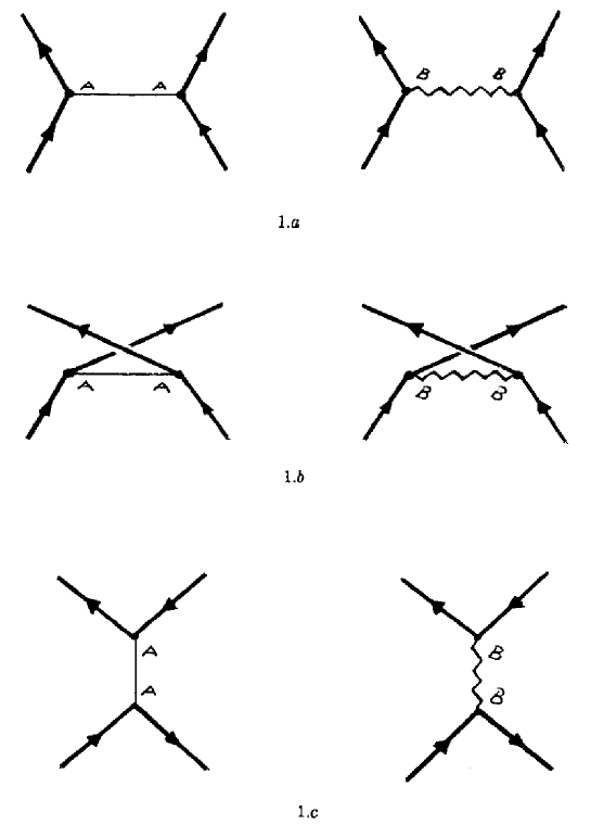
Figure 1: Lowest order graphs contributing to the scattering of two Majorana fermions.

2.1 Tree Level Scattering

We first concentrate on the elastic scattering of two Majorana fermions. We shall designate by $p_{1},p_{2}$ ($p^{\prime}_{1},p^{\prime}_{2}$) and by $\epsilon_{1},\epsilon_{2}$ ($\epsilon^{\prime}_{1},\epsilon^{\prime}_{2}$) the four momenta and z-spin components of the incoming (outgoing) particles, respectively. The Feynman graphs contributing to this process, in the lowest order of perturbation theory, are those depicted in Fig.1 while the associated amplitude is given by $R=-i(2\pi)^{4}\delta^{(4)}(p^{\prime}_{1}+p^{\prime}_{2}-p_{1}-p_{2})\,T$, where $T=T_{a}+T_{b}+T_{c}$ and

$$T_{a}\, = \,K\,\cos(p^{\prime}_{1}\wedge p_{1})\,\cos(p^{\prime}_{2}\wedge p_{2})\,\frac{\left(F_{a}-F_{a}^{5}\right)}{{\cal D}_{a}},$$ (2.3a)

$$T_{b}\, = \,-\,K\,\cos(p^{\prime}_{1}\wedge p_{2})\,\cos(p^{\prime}_{2}\wedge p_{1})\,\frac{\left(F_{b}-F_{b}^{5}\right)}{{\cal D}_{b}},$$ (2.3b)

$$T_{c}\, = \,K\,\cos(p^{\prime}_{1}\wedge p^{\prime}_{2})\,\cos(p_{1}\wedge p_{2})\,\frac{\left(F_{c}-F_{c}^{5}\right)}{{\cal D}_{c}}.$$ (2.3c)

The correspondence between the sets of graphs $a,b,c$, in Fig.1, and the partial amplitudes $T_{a},T_{b},T_{c}$ is self explanatory. Furthermore,

$$F_{a}\equiv\left[{\bar{u}}(\vec{p}\,^{\prime}_{1},\epsilon^{\prime}_{1})u(\vec{p}_{1},\epsilon_{1})\right]\left[{\bar{u}}(\vec{p}\,^{\prime}_{2},\epsilon^{\prime}_{2})u(\vec{p}_{2},\epsilon_{2})\right],$$ (2.4a)

$$F_{a}^{5}\equiv\left[{\bar{u}}(\vec{p}\,^{\prime}_{1},\epsilon^{\prime}_{1})\gamma^{5}u(\vec{p}_{1},\epsilon_{1})\right]\left[{\bar{u}}(\vec{p}\,^{\prime}_{2},\epsilon^{\prime}_{2})\gamma^{5}u(\vec{p}_{2},\epsilon_{2})\right],$$ (2.4b)

$${\cal D}_{a}\equiv\left(p^{\prime}_{1}-p_{1}\right)^{2}\,-\,m^{2}\,+\,i\epsilon,$$ (2.4c)

$$F_{b}\equiv\left[{\bar{u}}(\vec{p}\,^{\prime}_{1},\epsilon^{\prime}_{1})u(\vec{p}_{2},\epsilon_{2})\right]\left[{\bar{u}}(\vec{p}\,^{\prime}_{2},\epsilon^{\prime}_{2})u(\vec{p}_{1},\epsilon_{1})\right],$$ (2.4d)

$$F_{b}^{5}\equiv\left[{\bar{u}}(\vec{p}\,^{\prime}_{1},\epsilon^{\prime}_{1})\gamma^{5}u(\vec{p}_{2},\epsilon_{2})\right]\left[{\bar{u}}(\vec{p}\,^{\prime}_{2},\epsilon^{\prime}_{2})\gamma^{5}u(\vec{p}_{1},\epsilon_{1})\right],$$ (2.4e)

$${\cal D}_{b}\equiv\left(p^{\prime}_{1}-p_{2}\right)^{2}\,-\,m^{2}\,+\,i\epsilon,$$ (2.4f)

$$F_{c}\equiv\left[{\bar{u}}(\vec{p}\,^{\prime}_{1},\epsilon^{\prime}_{1})v(\vec{p}\,^{\prime}_{2},\epsilon^{\prime}_{2})\right]\left[{\bar{v}}(\vec{p}_{2},\epsilon_{2})u(\vec{p}_{1},\epsilon_{1})\right],$$ (2.4g)

$$F_{c}^{5}\equiv\left[{\bar{u}}(\vec{p}\,^{\prime}_{1},\epsilon^{\prime}_{1})\gamma^{5}v(\vec{p}\,^{\prime}_{2},\epsilon^{\prime}_{2})\right]\left[{\bar{v}}(\vec{p}_{2},\epsilon_{2})\gamma^{5}u(\vec{p}_{1},\epsilon_{1})\right],$$ (2.4h)

$${\cal D}_{c}\equiv\left(p_{1}+p_{2}\right)^{2}\,-\,m^{2}\,+\,i\epsilon,$$ (2.4i)

$$K\,=\,\frac{1}{\pi^{2}}\,\frac{g^{2}}{(2\pi)^{4}}\,\frac{m^{2}}{\sqrt{\omega(\vec{p}\,^{\prime}_{1})\omega(\vec{p}\,^{\prime}_{2})\omega(\vec{p}_{1})\omega(\vec{p}_{2})}},$$ (2.5)

and $\omega(\vec{p})\equiv{\sqrt{\vec{p}^{\,2}+m^{2}}}$. Here, the $u$’s and the $v$’s are, respectively, complete sets of positive and negative energy solutions of the free Dirac equation. Besides orthogonality and completeness conditions they also obey

$$C\,{\bar{u}}^{T}(\vec{p},\epsilon)\,=\,v(\vec{p},\epsilon),$$ (2.6a)

$$C\,{\bar{v}}^{T}(\vec{p},\epsilon)\,=\,u(\vec{p},\epsilon),$$ (2.6b)

where $C\equiv i\gamma^{2}\gamma^{0}$ is the charge conjugation matrix and ${\bar{u}}^{T}$ (${\bar{v}}^{T}$) denotes the transpose of ${\bar{u}}$ (${\bar{v}}$). Explicit expressions for these solutions can be found in Ref.[30].

Now, Majorana particles and antiparticles are identical and, unlike the case for Dirac fermions, all diagrams in Fig. 1 contribute to the elastic scattering amplitude of two Majorana quanta. Then, before going further on, we must verify that the spin-statistics connection is at work. As expected, $T_{a}+T_{b}$ undergoes an overall change of sign when the quantum numbers of the particles in the outgoing (or in the incoming) channel are exchanged (see Eqs. (2.3a) and (LABEL:4)). As for $T_{c}$, we notice that

$${\bar{u}}(p,\epsilon)v(p^{\prime},\epsilon^{\prime})\,=\,-\,{\bar{u}}(p^{\prime},\epsilon^{\prime})v(p,\epsilon),$$ (2.7a)

$${\bar{u}}(p,\epsilon)\gamma^{5}v(p^{\prime},\epsilon^{\prime})\,=\,-\,{\bar{u}}(p^{\prime},\epsilon^{\prime})\gamma^{5}v(p,\epsilon),$$ (2.7b)

are just direct consequences of Eq.(LABEL:6). Thus, $T_{c}$, alone, also changes sign under the exchange of the outgoing (or incoming) particles and, therefore, $T_{a}+T_{b}+T_{c}$ is antisymmetric.

The main purpose in this paper is to disentangle the relevant features of the low energy regime of the NC WZ model. Since noncommutativity breaks Lorentz invariance, we must carry out this task in an specific frame of reference that we choose to be the center of mass (CM) frame. Here, the two body kinematics becomes simpler because one has that $p_{1}=(\omega,\vec{p})$, $p_{2}=(\omega,-\vec{p})$, $p^{\prime}_{1}=(\omega,\vec{p}\,^{\prime})$, $p^{\prime}_{2}=(\omega,-\vec{p}\,^{\prime})$, $|\vec{p}\,^{\prime}|=|\vec{p}\,|$, and $\omega=\omega(\vec{p})$. This facilitates the calculation of all terms of the form

$$\left[\frac{m}{\pi\omega(\vec{p})}\right]^{2}\,\frac{\left(F-F^{5}\right)}{{\cal D}},$$ (2.8)

in Eqs.(2.3a). By disregarding all contributions of order $(|\vec{p}\,|/m)^{2}$ and higher, and after some algebra one arrives at

$$T^{L}_{a}\, = \,-\frac{1}{(2\pi)^{4}}\,\left(\frac{g}{\pi\,m}\right)^{2}\,\delta_{\epsilon^{\prime}_{1}\epsilon_{1}}\,\delta_{\epsilon^{\prime}_{2}\epsilon_{2}}\,\left[\frac{1}{2}\cos\left(m\Theta_{0j}k^{j}\right)\,+\,\frac{1}{2}\cos\left(p^{i}\Theta_{ij}k^{j}\right)\right]\,,$$ (2.9a)

$$T^{L}_{b}\, = \,\,\frac{1}{(2\pi)^{4}}\,\left(\frac{g}{\pi\,m}\right)^{2}\,\delta_{\epsilon^{\prime}_{1}\epsilon_{2}}\,\delta_{\epsilon^{\prime}_{2}\epsilon_{1}}\,\left[\frac{1}{2}\cos\left(m\Theta_{0j}k^{\prime}\,{}^{j}\right)\,+\,\frac{1}{2}\cos\left(p^{i}\Theta_{ij}k^{\prime}\,{}^{j}\right)\right]\,,$$ (2.9b)

$$T^{L}_{c}\, = \,\,\frac{1}{3(2\pi)^{4}}\,\left(\frac{g}{\pi\,m}\right)^{2}\,\left\{\delta_{\epsilon^{\prime}_{1}\epsilon_{1}}\,\delta_{\epsilon^{\prime}_{2}\epsilon_{2}}\,\cos\left(m\Theta_{0j}p^{j}\right)\cos\left[m\Theta_{0j}\left(p^{j}-k^{j}\right)\right]\right.$$ (2.9c)

$$\left.-\,\delta_{\epsilon^{\prime}_{1}\epsilon_{2}}\,\delta_{\epsilon^{\prime}_{2}\epsilon_{1}}\,\cos\left(m\Theta_{0j}p^{j}\right)\cos\left[m\Theta_{0j}\left(p^{j}-k^{\prime}\,{}^{j}\right)\right]\right\}\,,$$

where $k^{j}\equiv p^{j}-p^{\prime}\,{}^{j}$ ($k^{\prime}\,{}^{j}\equiv p^{j}+p^{\prime}\,{}^{j}$) denotes the momentum transferred in the direct (exchange) scattering while the superscript $L$ signalizes that the above expressions only hold true for the low energy regime. It is worth mentioning that the dominant contributions to $T^{L}_{a}$ and $T^{L}_{b}$ are made by those diagrams in Fig. 1$a$ and Fig.1$b$ not containing the vertices $i\gamma^{5}$, while, on the other hand, the dominant contribution to $T^{L}_{c}$ comes from the diagram in Fig.1$c$ with vertices $i\gamma^{5}$. Clearly, $T^{L}_{a}+T^{L}_{b}+T^{L}_{c}$ is antisymmetric under the exchange $\epsilon_{1}^{\prime}\leftrightarrow\epsilon^{\prime}_{2}$, $\vec{p}\,^{\prime}\rightarrow-\vec{p}\,^{\prime}$ ($k^{j}\leftrightarrow k^{\prime}\,{}^{j}$), as it must be. Also notice that, in the CM frame of reference, only the cosine factors introduced by the time/space noncommutativity are present in $T^{L}_{c}$.

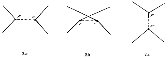
Figure 2: Lowest order graphs contributing to the scattering of two $A$-quanta.

We look next for the elastic scattering amplitude involving two $A$-field quanta. The diagrams contributing to this process, in the lowest order of perturbation theory, are depicted in Fig.2. The corresponding (symmetric) amplitude, already written in the CM frame of reference, can be cast as ${\bar{R}}=-i(2\pi)^{4}\delta^{(4)}(p^{\prime}_{1}+p^{\prime}_{2}-p_{1}-p_{2})\,{\bar{T}}$, where ${\bar{T}}={\bar{T}}_{a}+{\bar{T}}_{b}+{\bar{T}}_{c}$ and

$${\bar{T}}_{a}\, = \,\,\frac{g^{2}}{(2\pi)^{4}}\,\left(\frac{1}{2\pi\omega(\vec{p})}\right)^{2}\,\left[\frac{1}{2}\cos\left(m\Theta_{0j}k^{j}\right)\,+\,\frac{1}{2}\cos\left(p^{i}\Theta_{ij}k^{j}\right)\right]\,\frac{1}{\bar{\cal D}}_{a},$$ (2.10a)

$${\bar{T}}_{b}\, = \,\,\frac{g^{2}}{(2\pi)^{4}}\,\left(\frac{1}{2\pi\omega(\vec{p})}\right)^{2}\,\left[\frac{1}{2}\cos\left(m\Theta_{0j}k^{\prime}\,{}^{j}\right)\,+\,\frac{1}{2}\cos\left(p^{i}\Theta_{ij}k^{\prime}\,{}^{j}\right)\right]\,\frac{1}{\bar{\cal D}}_{b},$$ (2.10b)

$${\bar{T}}_{c}\, = \,\,\frac{g^{2}}{2(2\pi)^{4}}\,\left(\frac{1}{2\pi\omega(\vec{p})}\right)^{2}\,\left\{\cos\left(m\Theta_{0j}p^{j}\right)\cos\left[m\Theta_{0j}\left(p^{j}-k^{j}\right)\right]\right.$$ (2.10c)

$$\left.+\cos\left(m\Theta_{0j}p^{j}\right)\cos\left[m\Theta_{0j}\left(p^{j}-k^{\prime}\,{}^{j}\right)\right]\right\}\,\frac{1}{\bar{\cal D}}_{c}\,.$$

As far as the low energy limit is concerned, the main difference between the fermionic and bosonic scattering processes rests, roughly speaking, on the structure of the propagators mediating the interaction. Indeed, the propagators involved in the fermionic amplitude are those of the fields $A$ and $B$, namely[18],

$$\Delta_{AA}(p)\,=\,\Delta_{BB}(p)\,=\,i\,{\cal D}^{-1}(p)\,=\,\frac{i}{p^{2}-m^{2}+i\epsilon},$$ (2.11)

which, in all the three cases (a, b, and c), yield a nonvanishing contribution at low energies (see Eqs.(2.4c), (2.4f) and (2.4i)). On the other hand, the propagator involved in the bosonic amplitude is that of the $F$-field, i.e.[18],

$$\Delta_{FF}\,=\,i\,{\bar{\cal D}}^{-1}(p)\,=\,i\,\frac{p^{2}}{p^{2}-m^{2}+i\epsilon},$$ (2.12)

which in turns implies that

$${\bar{\cal D}}_{a}^{-1}\,=\,\frac{2\,\biggl{|}\frac{\vec{p}}{m}\biggr{|}^{2}\,\left(1-\cos\theta\right)}{1+2\,\biggl{|}\frac{\vec{p}}{m}\biggr{|}^{2}\,\left(1-\cos\theta\right)}\,=\,{\cal O}\left(\biggl{|}\frac{\vec{p}}{m}\biggr{|}^{2}\right),$$ (2.13a)

$${\bar{\cal D}}_{b}^{-1}\,=\,\frac{2\,\biggl{|}\frac{\vec{p}}{m}\biggr{|}^{2}\,\left(1+\cos\theta\right)}{1+2\,\biggl{|}\frac{\vec{p}}{m}\biggr{|}^{2}\,\left(1+\cos\theta\right)}\,=\,{\cal O}\left(\biggl{|}\frac{\vec{p}}{m}\biggr{|}^{2}\right),$$ (2.13b)

$${\bar{\cal D}}_{c}^{-1}\,=\,\frac{4\,+\,4\,\biggl{|}\frac{\vec{p}}{m}\biggr{|}^{2}\,}{3+4\,\biggl{|}\frac{\vec{p}}{m}\biggr{|}^{2}}\,=\,\frac{4}{3}\,\left[1+{\cal O}\left(\biggl{|}\frac{\vec{p}}{m}\biggr{|}^{2}\right)\right].$$ (2.13c)

Therefore, at the limit where all the contributions of order $(|\vec{p}\,|/m)^{2}$ become neglectable, the amplitudes ${\bar{T}}_{a}$ and ${\bar{T}}_{b}$ vanish whereas ${\bar{T}}_{c}$ survives and is found to read

$${\bar{T}}^{L}_{c}=\frac{1}{6(2\pi)^{4}}\left(\frac{g}{\pi m}\right)^{2}\cos\left(m\Theta_{0j}p^{j}\right)\left\{\cos\left[m\Theta_{0j}\left(p^{j}-k^{j}\right)\right]+\cos\left[m\Theta_{0j}\left(p^{j}-k^{\prime}\,{}^{j}\right)\right]\right\}.$$ (2.14)

2.2 The Effective Quantum Mechanical Potential

We shall next start thinking of the amplitudes in Eqs.(2.9a) and (2.14) as of scattering amplitudes deriving from a set of potentials. These potentials are defined as the Fourier transforms (FT), with respect to the transferred momentum ($\vec{k}$), of the respective direct scattering amplitudes. This is due to the fact that the use, in nonrelativistic quantum mechanics, of antisymmetric wave functions for fermions and of symmetric wave functions for bosons automatically takes care of the contributions due to exchange scattering[26]. Whenever the amplitudes depend only on $\vec{k}$ the corresponding FT will be local, depending only on a relative coordinate $\vec{r}$. However, if, as it happens here, the amplitudes depend not only on $\vec{k}$ but also on the initial momentum of the scattered particle $(\vec{p})$, the FT will be a function of both $\vec{r}$ and $\vec{p}$. As the momentum and position operators do not commute the construction of potential operators from these FT may be jeopardized by ordering problems. In that situation, we will proceed as follows: In the FT of the amplitudes we promote the relative coordinate and momentum to noncommuting canonical conjugated variables and then solve possible ordering ambiguities by requiring hermiticity of the resulting expression. A posteriori, we shall verify that this is in fact an effective potential in the sense that its momentum space matrix elements correctly reproduce the scattering amplitudes that we had at the very start of this construction.

We are, therefore, led to introduce

$$\delta_{\epsilon^{\prime}_{1}\epsilon_{1}}\,\delta_{\epsilon^{\prime}_{2}\epsilon_{2}}\,{\cal M}^{F}(\vec{k},\vec{p})\,\equiv\,T_{a}^{L}(\vec{k},\vec{p})\,+\,T_{c,dir}^{L}(\vec{k},\vec{p})\,$$ (2.15)

and

$${\cal M}^{B}(\vec{k},\vec{p})\,\equiv\,{\bar{T}}_{c,dir}^{L}(\vec{k},\vec{p})\,,$$ (2.16)

in terms of which the desired FT ($V^{F}$ and $V^{B}$) are given by

$$V^{F,B}({\vec{r}},\vec{p})\,=\,(2\pi)^{3}\,\int d^{3}k\,{\cal M}^{F,B}(\vec{k},\vec{p})\,e^{i\vec{k}\cdot{\vec{r}}}.$$ (2.17)

In the equations above, the superscripts $F$ and $B$ identify, respectively, the fermionic and bosonic amplitudes and Fourier transforms. Also, the subscript $dir$ specifies that only the direct pieces of the amplitudes $T_{c}^{L}$ and ${\bar{T}}_{c}^{L}$ enter in the calculation of the respective ${\cal M}$. Once $V^{F,B}({\vec{r}},\vec{p})$ have been found one has to look for their corresponding quantum operators, ${\hat{V}}^{F,B}\,({\vec{R}},{\vec{P}})$, by performing the replacements ${\vec{r}}\rightarrow{\vec{R}},{\vec{p}}\rightarrow{\vec{P}}$, where $\vec{R}$ and $\vec{P}$ are the Cartesian position and momentum operators obeying, by assumption, the canonical commutation relations $\left[R^{j},R^{l}\right]=\left[P^{j},P^{l}\right]=0$ and $\left[R^{j},P^{l}\right]=i\,\delta^{jl}$. By putting all this together one is led to the Hermitean forms

$${\hat{V}}^{F}({\vec{R}},{\vec{P}})\, = \,-\,\left(\frac{g}{m}\right)^{2}\,\int\frac{d^{3}k}{(2\pi)^{3}}\left(e^{ik^{l}R^{l}}\,e^{ik^{l}\Theta_{lj}P^{j}}+e^{ik^{l}R^{l}}\,e^{-ik^{l}\Theta_{lj}P^{j}}\right)$$

$$- \,\frac{2}{3}\left(\frac{g}{m}\right)^{2}\,\left[\delta^{(3)}\left({\vec{R}}+m{\vec{\Theta}}\right)\,+\,\delta^{(3)}\left({\vec{R}}-m{\vec{\Theta}}\right)\right]$$ (2.18)

$$+ \,\frac{1}{3}\left(\frac{g}{m}\right)^{2}\,\left[\,\delta^{(3)}\left({\vec{R}}-m{\vec{\Theta}}\right)\,e^{-2im{\vec{\Theta}}\cdot{\vec{P}}}\,+\,e^{2im{\vec{\Theta}}\cdot{\vec{P}}}\,\delta^{(3)}\left({\vec{R}}-m{\vec{\Theta}}\right)\right]\,,$$

$${\hat{V}}^{B}({\vec{R}},{\vec{P}})\, = \,\frac{1}{6}\left(\frac{g}{m}\right)^{2}\,\left[\delta^{(3)}\left({\vec{R}}+m{\vec{\Theta}}\right)\,+\,\delta^{(3)}\left({\vec{R}}-m{\vec{\Theta}}\right)\right]$$ (2.19)

$$+ \,\frac{1}{6}\left(\frac{g}{m}\right)^{2}\,\left[\delta^{(3)}\left({\vec{R}}-m{\vec{\Theta}}\right)\,e^{-2im{\vec{\Theta}}\cdot{\vec{P}}}\,+\,e^{2im{\vec{\Theta}}\cdot{\vec{P}}}\,\delta^{(3)}\left({\vec{R}}-m{\vec{\Theta}}\right)\right]\,,$$

where ${\vec{\Theta}}\equiv\{\Theta^{0j},j=1,2,3\}$. Notice that the magnetic components of $\Theta_{\mu\nu}$, namely $\Theta_{ij}$, only contribute to ${\hat{V}}^{F}$ and that such contribution is free of ordering ambiguities, since

$$\left[k^{l}R^{l}\,,\,k^{m}\Theta_{mj}P^{j}\right]\,=\,i\,k^{l}\,k^{m}\,\Theta_{mj}\,\delta^{lj}\,=\,0,$$ (2.20)

in view of the antisymmetry of $\Theta_{mj}$. On the other hand, the contributions to ${\hat{V}}^{F}$ and ${\hat{V}}^{B}$ originating in the electric components of $\Theta_{\mu\nu}$, namely $\Theta_{0j}$, are afflicted by ordering ambiguities. The relevant point is that there exist a preferred ordering that makes ${\hat{V}}^{F}$ and ${\hat{V}}^{B}$ both Hermitean, for arbitrary $\Theta_{\mu\nu}$. Equivalent forms to those presented in Eqs.(2.2) and (2.19) can be obtained by using

$$\delta^{(3)}\left({\vec{R}}-m{\vec{\Theta}}\right)\,\exp\left(-2im{\vec{\Theta}}\cdot{\vec{P}}\right)\,=\,\exp\left(-2im{\vec{\Theta}}\cdot{\vec{P}}\right)\,\delta^{(3)}\left({\vec{R}}+m{\vec{\Theta}}\right)\,.$$ (2.21)

We shall shortly verify that the matrix elements of the operators (2.2) and (2.19) agree with the original scattering amplitudes. Before that, however, we want to make some observations about physical aspects of these operators.

We will consider, separately, the cases of space/space ($\Theta_{0j}=0$) and time/space ($\Theta_{ij}=0$) noncommutativity. Hence, we first set $\Theta_{0j}=0$ in Eqs.(2.2) and (2.19). As can be seen, the potential ${\hat{V}}^{B}$, mediating the interaction of two $A$ quanta, remains as in the commutative case, i.e., proportional to a delta function of the relative distance between them. The same conclusion applies, of course, to the elastic scattering of two $B$ quanta. In short, taking the nonrelativistic limit also implies in wiping out all the modifications induced by the space/space noncommutativity on the bosonic scattering amplitudes. On the contrary, Majorana fermions are sensitive to the presence of space/space noncommutativity. Indeed, from Eq.(2.2) follows that ${\hat{V}}^{F}$ can be split into planar (${\hat{V}}^{F}_{P}$) and nonplanar (${\hat{V}}^{F}_{NP}$) parts depending on whether or not they depend on $\Theta_{ij}$, i.e.,

$${\hat{V}}^{F}({\vec{R}},{\vec{P})}\,=\,{\hat{V}}^{F}_{P}(\vec{R},{\vec{P}})\,+\,{\hat{V}}^{F}_{NP}(\vec{R},{\vec{P}})\,,$$ (2.22)

with

$${\hat{V}}^{F}_{P}(\vec{R})\, = \,-\,\frac{{2}}{3}\,\left(\frac{g}{m}\right)^{2}\,\delta^{(3)}(\vec{R})\,,$$ (2.23a)

$${\hat{V}}^{F}_{NP}(\vec{R},\vec{P})\, = \,-\,\left(\frac{g}{m}\right)^{2}\int\,\frac{d^{3}k}{(2\pi)^{3}}\left[\exp\left(ik^{l}R^{l}\right)\,\exp\left(ik^{l}\Theta_{lj}P^{j}\right)\right.$$ (2.23b)

$$\left.+\exp\left(ik^{l}R^{l}\right)\,\exp\left(-ik^{l}\Theta_{lj}P^{j}\right)\right]\,.$$

For further use in the Schrödinger equation, we shall be needing the position representation of ${\hat{V}^{F}}\left(\vec{R},\vec{P}\right)$. ¿From (2.23a) one easily sees that $<\vec{r}\,|{\hat{V}^{F}}_{P}|\vec{r}\,^{\prime}>=-{2}/3\,(g/m)^{2}\,\delta^{(3)}(\vec{r})\,\delta^{(3)}(\vec{r}-\vec{r}\,^{\prime})$. On the other hand, for the computation of $<\vec{r}\,|{\hat{V}^{F}}_{NP}|\vec{r}\,^{\prime}>$ it will prove convenient to introduce the realization of $\Theta_{ij}$ in terms of the magnetic field $\vec{B}$, i.e.,

$$\Theta_{ij}\,=\,-\,\epsilon_{ijk}\,B^{k}\,,$$ (2.24)

where $\epsilon_{ijk}$ is the fully antisymmetric Levi-Civita tensor ($\epsilon^{123}=+1$). After straightforward calculations one arrives at

$$<\vec{r}\,|{\hat{V}^{F}}_{NP}|\vec{r}\,^{\prime}>\,=\,-\frac{2}{(2\pi)^{2}}\,\left(\frac{g}{m}\right)^{2}\,\frac{1}{B^{2}}\,\delta^{(1)}({\vec{r}}_{\parallel})\,\delta^{(1)}({\vec{r}}_{\parallel}-{\vec{r}}\,^{\prime}_{\parallel})\,\cos\left[\frac{\left({\vec{r}}_{\perp}\times{\vec{r}}\,^{\prime}_{\perp}\right)\cdot{\vec{B}}}{B^{2}}\right]\,.$$ (2.25)

Here, ${\vec{r}}_{\parallel}$ (${\vec{r}}_{\perp}$) denotes the component of ${\vec{r}}$ parallel (perpendicular) to ${\vec{B}}$, i.e., ${\vec{r}}_{\parallel}=({\vec{r}}\cdot{\vec{B}}){\vec{B}}/B^{2}$ (${\vec{r}}_{\perp}=-({\vec{r}}\times{\vec{B}})\times{\vec{B}}/B^{2}$). We remark that the momentum space matrix element

$$<\vec{p}\,^{\prime}|{\hat{V}}^{F}_{NP}|\vec{p}>\,=\,\int d^{3}r\int d^{3}r^{\prime}<\vec{p}\,^{\prime}|{\vec{r}}><{\vec{r}}\,|{\hat{V}}^{F}_{NP}|{\vec{r}}\,^{\prime}><{\vec{r}}\,^{\prime}|\vec{p}>$$ (2.26)

$$= \,-\,\frac{1}{(2\pi)^{3}}\,\left(\frac{g}{mB}\right)^{2}\,\int d^{2}r_{\perp}\,\exp\left(-i{\vec{p}}\,^{\prime}_{\perp}\cdot{\vec{r}}_{\perp}\right)$$

$$\times \left\{\delta^{(2)}\left[{\vec{p}}_{\perp}-\left({\vec{r}}_{\perp}\times\frac{{\vec{B}}}{B^{2}}\right)\right]\,+\,\delta^{(2)}\left[{\vec{p}}_{\perp}+\left({\vec{r}}_{\perp}\times\frac{{\vec{B}}}{B^{2}}\right)\right]\right\}$$

$$= -\,\frac{1}{4\pi^{3}}\,\left(\frac{g}{m}\right)^{2}\,\cos\left[\left({\vec{p}}_{\perp}\times{\vec{p}}\,^{\prime}_{\perp}\right)\cdot{\vec{B}}\right]\,$$

agrees with the last term in (2.9a), as it should. We also observe that the interaction only takes place at ${\vec{r}}_{\perp}=\pm{\vec{B}}\times{\vec{p}}_{\perp}$. This implies that ${\vec{r}}_{\perp}$ must also be orthogonal to ${\vec{p}}_{\perp}$. Hence, in the case of space/space noncommutativity fermions may be pictured as rods oriented perpendicular to the direction of the incoming momentum. Furthermore, the right hand side of this last equation vanishes if either ${\vec{p}}_{\perp}\times{\vec{p}}\,^{\prime}_{\perp}=0$, or $\left({\vec{p}}_{\perp}\times{\vec{p}}\,^{\prime}_{\perp}\right)\cdot{\vec{B}}=0$, or $\vec{p}=\vec{p}_{\parallel}$, or $\vec{p}\,^{\prime}=\vec{p}\,^{\prime}_{\parallel}$.

In the Born approximation, the fermion-fermion elastic scattering amplitude ($f^{F}({\vec{p}}\,^{\prime},{\vec{p}})$) can be computed at once, since $f^{F}({\vec{p}}\,^{\prime},{\vec{p}})=-4\pi^{2}m<\vec{p}\,^{\prime}|{\hat{V}}^{F}|\vec{p}>$. In turns, the corresponding outgoing scattering state ($\Phi^{F(+)}_{\vec{p}}(\vec{r})$) is found to behave asymptotically ($r\rightarrow\infty$) as follows

$$e^{-iEt}\,\Phi^{F(+)}_{\vec{p}}(\vec{r})\,\sim\,\left(\frac{1}{2\pi}\right)^{\frac{3}{2}}\left[e^{-i\left(Et-\vec{p}\cdot{\vec{r}}\right)}\,+\,\frac{e^{-i\left(Et-pr\right)}}{r}\,f^{F}({\vec{p}}\,^{\prime},{\vec{p}})\right]$$ (2.27)

$$\sim \left(\frac{1}{2\pi}\right)^{\frac{3}{2}}\left\{e^{-i\left(Et-\vec{p}\cdot{\vec{r}}\,\right)}+\,\frac{g^{2}}{3\pi m}\frac{e^{-i(Et-pr)}}{r}\right.$$

$$\left.+\frac{g^{2}}{2\pi m}\,\left[\frac{e^{-i\left[Et-\left(\vec{p}_{\perp}\times\vec{p}\,^{\prime}_{\perp}\right)\cdot{\vec{B}}-pr\right]}}{r}\,+\,\frac{e^{-i\left[Et+\left(\vec{p}_{\perp}\times\vec{p}\,^{\prime}_{\perp}\right)\cdot{\vec{B}}-pr\right]}}{r}\right]\right\}\,,$$

where $E=\vec{p}^{2}/2m$ is the energy of the incoming particle. The right hand side of Eq.(2.27) contains three scattered waves. The one induced by the planar part of the potential (${\hat{V}}^{F}_{P}$) presents no time delay. The other two originate in the nonplanar part of the potential (${\hat{V}}^{F}_{NP}$) and exhibit time delays of opposite signs and proportional to $\left(\vec{p}_{\perp}\times\vec{p}\,^{\prime}_{\perp}\right)\cdot{\vec{B}}$. For instance, for ${\vec{B}}$ and ${\vec{p}}$ along the positive Cartesian semiaxis $x^{1}$ and $x^{3}$, respectively, one has that $\left(\vec{p}_{\perp}\times\vec{p}\,^{\prime}_{\perp}\right)\cdot{\vec{B}}\,=\,-2mEB\sin\theta\sin\phi$, were, $\theta$ and $\phi$ are the scattering and azimuthal angles, respectively. The $\phi$-dependence reflects the breaking of rotational invariance.

We set next $\Theta_{ij}=0$, in Eqs(2.2) and (2.19), and turn into analyzing the case of time/space noncommutativity. The effective potentials are now

$${\hat{\tilde{V}}}^{F}({\vec{R}},{\vec{P}})\, = \,-\,\frac{2}{3}\left(\frac{g}{m}\right)^{2}\,\left[\delta^{(3)}\left({\vec{R}}+m{\vec{\Theta}}\right)\,+\,\delta^{(3)}\left({\vec{R}}-m{\vec{\Theta}}\right)\right]$$ (2.28)

$$+ \,\frac{1}{3}\left(\frac{g}{m}\right)^{2}\,\left[\,\delta^{(3)}\left({\vec{R}}-m{\vec{\Theta}}\right)\,e^{-2im{\vec{\Theta}}\cdot{\vec{P}}}\,+\,e^{2im{\vec{\Theta}}\cdot{\vec{P}}}\,\delta^{(3)}\left({\vec{R}}-m{\vec{\Theta}}\right)\right]\,,$$

$${\hat{\tilde{V}}}^{B}({\vec{R}},{\vec{P}})\, = \,\frac{1}{6}\left(\frac{g}{m}\right)^{2}\,\left[\delta^{(3)}\left({\vec{R}}+m{\vec{\Theta}}\right)\,+\,\delta^{(3)}\left({\vec{R}}-m{\vec{\Theta}}\right)\right]$$ (2.29)

$$+ \,\frac{1}{6}\left(\frac{g}{m}\right)^{2}\,\left[\delta^{(3)}\left({\vec{R}}-m{\vec{\Theta}}\right)\,e^{-i2m{\vec{\Theta}}\cdot{\vec{P}}}\,+\,e^{i2m{\vec{\Theta}}\cdot{\vec{P}}}\,\delta^{(3)}\left({\vec{R}}-m{\vec{\Theta}}\right)\right]\,,$$

where the slight change in notation (${\hat{V}}\rightarrow{\hat{\tilde{V}}}$) is for avoiding confusion with the previous case. As before, we look first for the fermionic and bosonic elastic scattering amplitudes and then construct the asymptotic expressions for the corresponding scattering states. Analogously to (2.26) and (2.27) we find that

$$<\vec{p}\,^{\prime}|{\hat{\tilde{V}}}^{F}_{NP}|\vec{p}> = -\frac{1}{12\pi^{3}}\,\left(\frac{g}{m}\right)^{2}\left\{2\cos\left[m{\vec{\Theta}}\cdot\left(\vec{p}-\vec{p}\,^{\prime}\right)\right]\,-\,\cos\left[m{\vec{\Theta}}\cdot\left(\vec{p}+\vec{p}\,^{\prime}\right)\right]\right\}\,$$ (2.30)

and

$$e^{-iEt}\,{\tilde{\Phi}}_{\vec{p}}^{F(+)}{(\vec{r})}\, = \,\left(\frac{1}{2\pi}\right)^{\frac{3}{2}}\left\{e^{-i\left(Et-\vec{p}\cdot{\vec{r}}\right)}\right.$$ (2.31)

$$\left.+\,\frac{g^{2}}{3m\pi r}\,\left[{e^{-i\left[Et-m{\vec{\Theta}}\cdot\left(\vec{p}-\vec{p}\,^{\prime}\right)-pr\right]}}\,+\,{e^{-i\left[Et+m{\vec{\Theta}}\cdot\left(\vec{p}-\vec{p}\,^{\prime}\right)-pr\right]}}\right]\right.$$

$$\left.-\,\frac{g^{2}}{6m\pi r}\,\left[{e^{-i\left[Et-m{\vec{\Theta}}\cdot\left(\vec{p}+\vec{p}\,^{\prime}\right)-pr\right]}}\,+\,{e^{-i\left[Et+m{\vec{\Theta}}\cdot\left(\vec{p}+\vec{p}\,^{\prime}\right)-pr\right]}}\right]\right\}\,.$$

in accordance with the calculations of the section 2. As for the bosons, the potential in Eq.(2.29) leads to

$$<\vec{p}\,^{\prime}|{\hat{\tilde{V}}}^{B}_{NP}|\vec{p}>\, = \frac{1}{24\pi^{3}}\,\left(\frac{g}{m}\right)^{2}\,\,\left\{\cos\left[m{\vec{\Theta}}\cdot\left(\vec{p}-\vec{p}\,^{\prime}\right)\right]\,+\,\cos\left[m{\vec{\Theta}}\cdot\left(\vec{p}+\vec{p}\,^{\prime}\right)\right]\right\}\,$$ (2.32)

and

$$e^{-iEt}\,{\tilde{\Phi}}_{\vec{p}}^{B(+)}{(\vec{r})}\, = \,\left(\frac{1}{2\pi}\right)^{\frac{3}{2}}\Bigl{\{}e^{-i\left(Et-\vec{p}\cdot{\vec{r}}\right)}\Bigr{.}$$ (2.33)

$$\left.-\,\frac{g^{2}}{12m\pi r}\,\left[{e^{-i\left[Et-m{\vec{\Theta}}\cdot\left(\vec{p}-\vec{p}\,^{\prime}\right)-pr\right]}}\,+\,{e^{-i\left[Et+m{\vec{\Theta}}\cdot\left(\vec{p}-\vec{p}\,^{\prime}\right)-pr\right]}}\right.\right.$$

$$\left.\left.+\,{e^{-i\left[Et-m{\vec{\Theta}}\cdot\left(\vec{p}+\vec{p}\,^{\prime}\right)-pr\right]}}\,+\,{e^{-i\left[Et+m{\vec{\Theta}}\cdot\left(\vec{p}+\vec{p}\,^{\prime}\right)-pr\right]}}\right]\right\}\,.$$

We stress that, presently, the interaction only takes place at ${\vec{r}}=\pm(\vec{p}-\vec{p}\,^{\prime})/m^{2}$ and ${\vec{r}}=\pm(\vec{p}+\vec{p}\,^{\prime})/m^{2}$ (see Eqs.(2.30) and (2.32)). As consequence, particles in the forward and backward directions behave as rigid rods oriented along the direction of the incoming momentum $\vec{p}$. Furthermore, each scattering state (see Eqs.(2.31) and (2.33)) describes four scattered waves. Two of these waves are advanced, in the sense that the corresponding time delay is negative, analogously to what was found in [21].

3 One and Two Loop Corrections

Our study of the low energy limit of the noncommutative WZ model ends here. The main conclusion is that the quantum mechanics originating in this limit is always unitary. This is not in conflict with the existence of scattered advanced waves. Of course, this picture may change if loop contributions are taken into account. To see whether that really happens we shall employ the superfield approach, which is more appropriate for calculations involving higher orders in perturbation theory. This formulation has already been used to find the leading contributions to the effective action in one and two-loop orders in the case of the commutative WZ model [31, 32].

The superfield action for the NC WZ model is [28]

$$S\,=\,\int d^{8}z\,\bar{\Phi}\Phi\,-\,\left[\int d^{6}z\,\left(\frac{1}{2}m\Phi^{2}\,+\,\frac{g}{3!}\Phi*\Phi*\Phi\right)\,+\,h.c.\right]\,.$$ (3.34)

Here, $\Phi$ is a chiral superfield (for its component expansion see, for instance, Ref. [31]). Moreover, the Moyal product for superfields is defined as in Eq.(2). Notice that the noncommutativity does not involve the Grassmann coordinates. The propagators look as follows [31, 28]

$$<\Phi(z_{1}){\bar{\Phi}}(z_{2})>\, = \,\frac{-1}{\Box+m^{2}}\,\delta^{(8)}(z_{1}-z_{2})\,,$$ (3.35a)

$$<\Phi(z_{1})\Phi(z_{2})>\, = \,\frac{m}{4\Box}\,\frac{{D}^{2}}{\Box+m^{2}}\,\delta^{(8)}(z_{1}-z_{2})\,,$$ (3.35b)

where the $D$ factors are associated with vertices just by the same rules as in the commutative case. A chiral vertex, with $n$ external lines, carries $(2-n)$ factors $(-1/4){\bar{D}}^{2}$. In a similar way, an antichiral vertex carries $(2-n)$ factors $(-1/4){D}^{2}$. Furthermore, in momentum representation, any vertex also includes the factor $\cos(p_{1}\wedge p_{2})$, where $p_{1}$ and $p_{2}$ are two out of the three incoming momenta [28]. Just for comparison purposes we mention that the low energy direct scattering amplitudes associated with the supergraphs whose corresponding fermion component graphs are those given in Figs.1$a$, and 1$c$ read, respectively,

$$T^{S}_{a}\, = \,\left(\frac{g}{m}\right)^{2}\,\left(\frac{i}{\pi^{2}}\right)\,\frac{1}{(2\pi)^{4}}\,\int d^{4}\theta\,\,\Phi(m,\vec{p},\theta)\,{\bar{\Phi}}(m,-\vec{p},\theta)$$ (3.36a)

$$\Phi(m,\vec{p}\,^{\prime},\theta)\,{\bar{\Phi}}(m,-\vec{p}\,^{\prime},\theta)\left[\frac{1}{2}\cos\left(m\Theta_{0j}k^{j}\right)\,+\,\frac{1}{2}\cos\left(p^{i}\Theta_{ij}k^{j}\right)\right]\,,$$

$$T^{S}_{c}\, = \,-\,\frac{1}{3}\,\left(\frac{g}{m}\right)^{2}\,\left(\frac{i}{\pi^{2}}\right)\,\frac{1}{(2\pi)^{4}}\,\int d^{4}\theta\,\,\Phi(m,\vec{p},\theta)\,\Phi(m,-\vec{p},\theta)$$ (3.36b)

$${\bar{\Phi}}(m,\vec{p}\,^{\prime},\theta)\,{\bar{\Phi}}(m,-\vec{p}\,^{\prime},\theta)\cos\left(m\Theta_{0j}p^{j}\right)\cos\left[m\Theta_{0j}\left(p^{j}-k^{j}\right)\right]$$

where $T^{S}$ stands for superamplitudes. One can convince oneself that the effective potential arising from the amplitudes in Eq. (3.36a) reproduces those given in Eqs. (2.2) and (2.19). This is quite natural because in the low energy regime the fermionic sector receives only contributions from the above mentioned supergraphs. As for the low energy regime of the bosonic sector of interest ($A+A\rightarrow A+A$ and $B+B\rightarrow B+B$), the only contributions are those from supergraphs containing ${D}$ factors, which are responsible for the modifications of the propagator (see Eqs. (2.11) and (2.12)).

Let us focus on the one loop leading nonplanar contribution ($\Gamma_{NP}^{(1)}$) to the effective Lagrangian density, which is similar to that in the noncommutative $\phi^{3}$ scalar field theory. It can be shown that up to lowest order in $g$

$$\Gamma_{NP}^{(1)}\,=\,\frac{g^{2}}{4}\,\frac{1}{16\pi^{2}}\int_{0}^{1}dx\int\frac{d\alpha}{\alpha}e^{i\alpha[x(1-x)p^{2}-m^{2}]+i\frac{p\circ p}{4\alpha}-\alpha\epsilon}\Phi(-p,\theta)\bar{\Phi}(p,\theta)$$ (3.37)

Here, $p^{2}=p^{2}_{0}-p^{2}_{1}-p^{2}_{2}-p^{2}_{3}$ is the square of the norm of the Minkowskian four-vector $p$, while $p\circ p\equiv p^{\mu}\left(\Theta^{2}\right)_{\mu\nu}p^{\nu}$. Then, by means of an analysis similar to the one carried out in [22] for the case of the two-point function in the noncommutative scalar $\phi^{3}$ theory, we arrive to the conclusion that the unitarity constraint is violated whenever $p\circ p<0$. Since $p\circ p<0$ demands $\Theta_{0j}\neq 0$ [22], we conclude that time/space noncommutativity leads to a violation of unitarity.

Finally, we mention that the two-loop contribution to the nonplanar Kälherian effective potential ($\Phi=\mbox{constant}$) has already been found to read [33]

$$K^{(2)}_{NP}\,=\,\frac{1}{16\pi^{2}}\,\int_{0}^{\infty}\,\frac{d\alpha}{\alpha}\,\int_{0}^{1}dx\,\int_{0}^{\infty}\,dz\,e^{-i(\alpha+z)|m+g\Phi|^{2}}\,\int\frac{d^{4}k}{(2\pi)^{4}}\,e^{i[\alpha x(1-x)+z]k^{2}\,+\,i\frac{k\circ k}{4\alpha}}\,.$$ (3.38)

For time/space noncommutativity, this potential develops an imaginary part and therefore leads to a violation of unitarity.

To summarize, for the NC WZ model, unitarity is indeed violated within the relativistic regime. However, this does not preclude the existence of a unitary low energy regime.

References

• [1] M. R. Douglas and N. A. Nekrasov, “Noncommutative Field Theory”, hep-th/0106048.
• [2] R. J. Szabo, “Quantum Field Theory on Noncommutative Spaces”, hep-th/0109162.
• [3] S. Minwalla, M. V. Raamsdonk and N. Seiberg, “Noncommutative Perturbative Dynamics”, JHEP 02, 020 2000, hep-th/9912072.
• [4] I. Ya. Aref’eva, D. M. Belov and A. S. Koshelev, “Two–Loop Diagrams in Noncommutative $\varphi^{4}_{4}$ Theory”, Phys. Lett. B 476, 431 2000, hep-th/9912075.
• [5] I. Chepelev and R. Roiban, “Renormalization of Quantum Field Theories on Noncommutative $R^{D}$, 1. Scalars”, JHEP 0005, 037 2000, hep-th/9911098.
• [6] L. Griguolo and M. Pietroni, “Wilsonian Renormalization Group and the Noncommutative IR/UV Connection”, JHEP 0105, 032 2001, hep-th/0104217.
• [7] C. P. Martin and D. Sanchez-Ruiz, The one-loop UV divergent structure of U(1) Yang-Mills theory on NC $R^{4}$, Phys. Rev. Lett. 83 (1999) 476, hep-th/9903077.
• [8] H. B. Benaoum, Perturbative BF-Yang-Mills theory on NC $R^{4}$, Nucl. Phys. B585 (2000) 554, hep-th/9912036.
• [9] M. Hayakawa, Perturbative analysis on infrared and ultraviolet aspects of NC QED on $R^{4}$, hep-th/9912167; Perturbative analysis on infrared aspects of NC QED on $R^{4}$, Phys. Lett. B478 (2000) 394, hep-th/9912094.
• [10] M. Chaichian, M. M. Sheik-Jabbari and A. Tureanu, Hydrogen Atom Spectrum and the Lamb Shift in NC QED, hep-th/0001175.
• [11] H. Grosse, T. Krajewski, R. Wulkenhaar, Renormalization of NC Yang-Mills theories: a simple example, hep-th/0001182.
• [12] J. Madore, S. Schraml, P. Schupp, J. Wess, Gauge theories on NC spaces, Eur. Phys. J. C16 (2000) 161, hep-th/0001203.
• [13] A. Matusis, L. Susskind, N. Toumbas, The IR/UV connection in the NC gauge theories, hep-th/0002075.
• [14] L. Bonora, M. Schnabl and A. Tomasiello, A note on consistent anomalies in NC YM theories, Phys. Lett. B485 (2000) 311, hep-th/0002210.
• [15] A. Rajaraman and M. Rozali, NC Gauge Theory, Divergences and Closed Strings, JHEP 0004 (2000) 033, hep-th/0003227.
• [16] M. M. Sheikh-Jabbari, Renormalizability of the Supersymmetric Yang-Mills Theories on the NC Torus, JHEP 9906 (1999) 015, hep-th/9903107.
• [17] N. Grandi, R. L. Pakman and F. A. Schaposnik, “Supersymmetric Dirac-Born-Infeld Theory in Noncommutative Space”, Nuc. Phys. B588 (2000) 508, hep-th/0004104.
• [18] H. O. Girotti, M. Gomes, V. O. Rivelles, A. J. da Silva, “A consistent NC Field Theory: The Wess-Zumino Model”, Nucl. Phys. B587 (2000) 299, hep-th/0005272.
• [19] H. O. Girotti, M. Gomes, V. O. Rivelles and A. J. da Silva, ”The Noncommutative Supersymmetric Nonlinear Sigma Model”, hep-th/0102101, to appear in Int. J. Mod. Phys. A.; H. O. Girotti, M. Gomes, A. Yu. Petrov, V. O. Rivelles and A. J. da Silva, “The Three-Dimensional Noncommutative Nonlinear Sigma model in Superspace”, Phys. Lett. B521, (2001) 119.
• [20] D. Zanon, “Noncommutative Perturbation in Superspace”, Phys. Lett. B504 (2001) 101, hep-th/0009196.
• [21] N. Seiberg, L. Susskind and N. Toumbas, Space-time non-commutativity and causality, hep-th/0005015.
• [22] J. Gomis, T. Mehen, Space-time NC field theories and unitarity, Nucl. Phys. B591 (2000) 265, hep-th/0005129.
• [23] J. M. Gracia-Bondia and C. P. Martin, Chiral gauge anomalies on NC $R^{4}$, Phys. Lett. B479 (2000) 321, hep-th/0002171.
• [24] B. A. Campbell and K. Kaminsky NC Field Theory and Spontaneous Symmetry Breaking, Nucl. Phys. B581 (2000) 240, hep-th/0003137.
• [25] F. J. Petriello, The Higgs Mechanism in NC Gauge Theories, hep-th/0101109.
• [26] J. J. Sakurai, Advanced Quantum Mechanics, Addison-Wesley Publishing Co. (Ontario, 1967).
• [27] H. O. Girotti, M. Gomes, J. L. deLyra, R. S. Mendes, J. R. Nascimento and A. J. da Silva, Phys. Rev. Lett. 69 (1992) 2623; H. O. Girotti, M. Gomes and A. J. da Silva, Phys. Lett. B274 (1992) 357.
• [28] A. A. Bichl, J. M. Grimstrup, H. Grosse, L. Popp, M. Schweda and R. Wulkenhaar, The Superfield Formalism Applied to the NC Wess Zumino Model, JHEP 0010 (2000) 046, hep-th/0007050.
• [29] T. Filk, “Divergences in a Field Theory on Quantum Space”, Phys. Lett. B376, 53 1996.
• [30] H. J. W. Muller-Kirsten, Supersymmetry: an introduction with conceptual and calculational details , World Scientific, 1987.
• [31] I.L. Buchbinder, S.M. Kuzenko. Ideas and Methods of Supersymmetry and Supergravity or a Walk Through Superspace, IOP Publishing, Bristol and Philadelphia, 1995 (second edition, 1998).
• [32] I. L. Buchbinder, S. M. Kuzenko, A. Yu. Petrov, Phys. Lett. B321 (1994) 372; Yad. Fiz. (Phys. Atom. Nucl.) 59 (1996) 157.
• [33] I. L. Buchbinder, M. Gomes, A. Yu. Petrov and V, Rivelles, “Superfield Effective Action in the Noncommutative Wess-Zumino Model”, Phys. Lett. B517 , 191 2001, hep-th/0107022.