RUNHETC-2001-02

LPM-01-01

January, 2001

Abstract

Liouville field theory is considered with boundary conditions corresponding to a quantization of the classical Lobachevskiy plane (i.e. euclidean version of $AdS_{2}$). We solve the bootstrap equations for the out-vacuum wave function and find an infinite set of solutions. This solutions are in one to one correspondence with the degenerate representations of the Virasoro algebra. Consistency of these solutions is verified by both boundary and modular bootstrap techniques. Perturbative calculations lead to the conclusion that only the “basic” solution corresponding to the identity operator provides a “natural” quantization of the Lobachevskiy plane.

1 Introduction

Liouville field theory (LFT) is widely considered as an appropriate field theoretic background for a certain universality class of two-dimensional quantum gravity. It has been demonstrated in numerous examples that in 2D the scaling limit of the so-called “dynamical triangulations” [1, 2, 3, 4] (which are in fact a discrete model of a two-dimensional surface with fluctuating geometry) in many cases can be described by appropriately applied LFT [5, 6, 7]

Local dynamics of LFT is determined by the action density

$$\mathcal{L}(z)=\frac{1}{4\pi}(\partial_{a}\phi(z))^{2}+\mu e^{2b\phi(z)}$$ (1.1)

where $\phi$ is the Liouville field and $b$ is a dimensionless parameter which, roughly speaking, determines the “rigidity” of a 2D surface to quantum fluctuations of the metric. Ordinarily $\exp(2b\phi(z))d^{2}z$ is interpreted as the quantum volume element of the fluctuating surface, parameter $\mu$ being the cosmological coupling constant. LFT is a conformal field theory with central charge

$$c_{L}=1+6Q^{2}$$ (1.2)

where $Q$ is yet another convenient parameter called the “background charge”

$$Q=b^{-1}+b$$ (1.3)

More details about the space of states in LFT, the set of local primary fields and local operator algebra can be found e.g. in [11].

Local equation of motion for (1.1)

$$\Delta\phi=4\pi\mu be^{2b\phi}$$ (1.4)

is the quantum version of the classic Liouville equation

$$\Delta\varphi=2R^{-2}e^{\varphi}$$ (1.5)

It describes locally a metric

$$ds^{2}=e^{\varphi(z)}\left|dz\right|^{2}$$ (1.6)

of constant negative curvature $-2R^{-2}$ in the isothermal (or conformal) coordinates. Classical situation arises in LFT if $b\rightarrow 0$. In this limit we identify the classical field $\varphi=2b\phi$ while $R^{-2}=4\pi\mu b^{2}$.

Discrete models of quantum gravity, such as the random triangulations or matrix models, typically deal with compact fluctuating surfaces of different topologies either with or without boundaries. This type of problems is most relevant in the string theory. In this context the main problem is somewhat different from that considered usually in field theory. Namely, observables of primary interest are the “integrated” correlation functions, which bear no coordinate dependence and can be rather called the “correlation numbers”. They are used to describe certain “deformations” or “flows” caused by relevant perturbations (see e.g. the reviews [8, 9] and [10] for more details). In many problems of this kind the discrete approaches presently appear more efficient then the field theoretic description based on LFT. In the discrete schemes the correlation functions naturally arise in the “integrated” form while the field theoretic approach implies a gauge fixing and gives the correlation functions as the functions of certain moduli (invariants of the complex structure in the case of LFT). These functions, although being themselves of considerable interest, should be yet integrated over the moduli space to produce the correlation numbers. Therefore in such problems of quantum gravity LFT still lags behind matrix models or other discrete approaches. Up to now only general scaling exponents and a limited set of correlation functions in simplest compact topologies can be predicted in LFT (see e.g. [9] and references therein).

It is well known that the Liouville equation (1.5) admits “basic” solution, which describes the geometry of infinite constant negative curvature surface, the so-called Lobachevskiy plane, or pseudosphere. This surface can be realized as the disk $\left|z\right|<1$ with metric (1.6) where

$$e^{\varphi(z)}=\frac{4R^{2}}{(1-z\bar{z})^{2}}$$ (1.7)

Here $R$ is interpreted as the radius of the pseudosphere. The points at the circle $\left|z\right|=1$ are infinitely far away from any internal point and form a one-dimensional infinity called the absolute. Geometry of the pseudosphere is described in detail in standard textbooks and here we will not go into further details like $SL(2,R)$ symmetry, geodesics etc. Let us mention only the so-called Poincaré model, where the same geometry is represented in the upper half plane of complex $\xi$ with the metric

$$e^{\varphi(\xi)}=\frac{R^{2}}{(\operatorname*{Im}\xi)^{2}}$$ (1.8)

It seems natural to expect that LFT, at least in the semi-classical regime $c_{L}>25$, also allows a solution corresponding to a quantization of this geometry. In this paper we present what we believe might be the solution to this problem. Surprisingly, we find an infinite set of different consistent solutions parameterized by a couple of positive integers $(m,n)$ (which can be put in natural correspondence with the degenerate representations of the Virasoro algebra). Only the set $(1,n)$ has a smooth behavior as $b\rightarrow 0$ and therefore can be literally called the “quantization” of (1.7). Remarkably, all the solutions of this $(1,n)$ series are indistinguishable in the classical limit (and even at the one-loop level), dependence on $n$ appearing only in two-loop corrections. However, actual higher loop calculations show that only the solution $(m,n)=(1,1)$ is consistent with the standard loop perturbation theory. Therefore we are inclined to interpret this last solution as the “basic” one, corresponding to a “natural” quantization of the Lobachevskiy plane. Although the nature of other solutions is still beyond our understanding (even of the “perturbative” series $(1,n)$, $n>1$) they probably can be speculated as describing different phases of quantum gravity.

In principle all local properties of a field theory are encoded in its operator product expansions. The latter are basically known in LFT (see [12, 11]). To have a complete description we also need certain information of what is happening “faraway” from the observer, i.e, about the boundary conditions at infinity. This information is encoded in the wave function of the state which “comes from infinity”, the so-called out-vacuum. In order, the out-vacuum wave function can be described as the set of vacuum expectation values (VEV’s) of all local fields in the theory. In conformal field theory, like LFT, it suffices to determine the VEV’s (or one-point functions) of all primary operators. The basic Liouville primaries are the exponential fields

$$V_{\alpha}=\exp(2\alpha\phi)$$ (1.9)

of dimensions $\Delta_{\alpha}=\alpha(Q-\alpha)$. Thus the set of VEV’s $\left\langle V_{\alpha}\right\rangle$ is just the complementary information we need to describe LFT in the pseudosphere geometry. In this paper we mainly concentrate on this characteristic.

The paper is arranged as follows. In sect.2 the bootstrap technique is applied to derive the one-point functions $\left\langle V_{\alpha}\right\rangle$. We observe that all the out-vacuums $(m,n)$, if considered as conformal boundary conditions at absolute, allow only finite set of boundary operators. In particular, the basic out-vacuum $(1,1)$ does not contain any boundary fields except the identity operator and its conformal descendents. Few simplest bulk-boundary structure constants are also derived in this section. Certain properties of the solutions are discussed in section 3. This includes perturbative expansions of the one-point functions and some evidence about the content of the boundary operators in the state $(m,n)$. In sect.4 one- and two-loop contributions to the one-point functions are evaluated in the framework of standard Feynmann diagram technique. At two loops these calculations agree with the expansion of the “basic” vacuum state $(1,1)$.

In sect.5 the powerful modular bootstrap technique is applied to verify the consistency of the proposed operator content at the out-vacuum states $(m,n)$. Partition function of an annulus with “boundaries” corresponding to different out-vacua $(m,n)$ is considered. It turns out that the modular invariance of this partition function perfectly agrees with the suggested operator content and can be further implemented for “finite” boundary conditions discussed in ref.[13].

With a finite set of boundary operators any two-point function in the bulk is constructed as a finite sum of four-point conformal blocks. In sect.6 we develop this construction explicitly for two simplest vacua $(1,1)$ and $(1,2)$ and verify numerically that it satisfies the bulk-boundary bootstrap. Some outlook and discussion is presented in sect.7.

2 One-point bootstrap

The basic assumption of the further development is that the out-vacuum state generated by the absolute of the pseudosphere is conformally invariant, i.e., consists of a superposition of the Ishibashi states [14]. The one-point functions of primary fields are nothing but the amplitudes of different Ishibashi primaries in the out-vacuum wave function.

In this section we will use the Poincaré model of the Lobachevskiy plane with complex coordinate $\xi$ in the upper half plane. Due to the conformal invariance the coordinate dependence of any one-point function is prescribed by the dimension of the operator

$$\left\langle V_{\alpha}(\xi)\right\rangle=\frac{U(\alpha)}{\left|\xi-\bar{\xi}\right|^{2\Delta_{\alpha}}}$$ (2.1)

Thus we will call coordinate independent function $U(\alpha)$ the one-point function and normalize it in the usual in field theory way $U(0)=1$.

Of course, local properties of LFT do not depend on the boundary conditions. In particular the set of (bulk) degenerate fields

$$\Phi_{m,n}=\exp\left(((1-m)b^{-1}+(1-n)b)\phi\right)$$ (2.2)

still exists for any pair of positive $m$ and $n$. Therefore one can make use of the trick applied by J.Teschner in the study of the operator algebra [15] (see also [16] for very similar discussions). Consider the following auxiliary two-point correlation function with the insertion of an operator $\Phi_{1,2}=V_{-b/2}$

$$G_{-b/2,\alpha}(\xi,\xi^{\prime})=\left\langle V_{-b/2}(\xi)V_{\alpha}(\xi^{\prime})\right\rangle$$ (2.3)

Degenerate fields have very special structure of the operator product expansions. In particular, the product $\Phi_{1,2}V_{\alpha}$ contains in the right hand side only two primary fields $V_{\alpha-b/2}$ and $V_{\alpha+b/2}$. Function (2.3) is therefore combined of two degenerate conformal blocks

$$G_{-b/2,\alpha}=\frac{\left|\xi^{\prime}-\bar{\xi}^{\prime}\right|^{2\Delta_{\alpha}-2\Delta_{12}}}{\left|\xi-\bar{\xi}^{\prime}\right|^{4\Delta_{a}}}\left[C_{+}(\alpha)U(\alpha-b/2)\mathcal{F}_{+}(\eta)+C_{-}(\alpha)U(\alpha+b/2)\mathcal{F}_{-}(\eta)\right]$$ (2.4)

In our normalization the special structure constants $C_{\pm}(\alpha)$ read explicitly [15, 13]

$$C_{+}(\alpha) =1$$ (2.5)

$$C_{-}(\alpha) =-\pi\mu\frac{\Gamma(2\alpha b-b^{2}-1)\Gamma(1-2\alpha b)\Gamma(1+b^{2})}{\Gamma(2+b^{2}-2\alpha b)\Gamma(2\alpha b)\Gamma(-b^{2})}$$

Degenerate conformal blocks $\mathcal{F}_{\pm}(\eta)$ are functions of the projective invariant

$$\eta=\frac{(\xi-\xi^{\prime})(\bar{\xi}-\bar{\xi}^{\prime})}{(\xi-\bar{\xi}^{\prime})(\bar{\xi}-\xi^{\prime})}$$ (2.6)

They are known explicitly and can be expressed in terms of hypergeometric functions

$$\mathcal{F}_{+}(\eta) =\eta^{\alpha b}(1-\eta)^{-b^{2}/2}{}_{1}F_{2}(2\alpha b-2b^{2}-1,-b^{2},2\alpha b-b^{2},\eta)$$ (2.7)

$$\mathcal{F}_{-}(\eta) =\eta^{1+b^{2}-\alpha b}(1-\eta)^{-b^{2}/2}{}_{1}F_{2}(-b^{2},1-2\alpha b,2+b^{2}-2\alpha b,\eta)$$

The same expression (2.4) can be rewritten also in terms of the cross-channel degenerate blocks $\mathcal{G}_{\pm}(\eta)$

$$G_{-b/2,\alpha}=\frac{\left|\xi^{\prime}-\bar{\xi}^{\prime}\right|^{2\Delta_{\alpha}-2\Delta_{12}}}{\left|\xi-\bar{\xi}^{\prime}\right|^{4\Delta_{a}}}\left[B^{(+)}(\alpha)\mathcal{G}_{+}(\eta)+B^{(-)}(\alpha)\mathcal{G}_{-}(\eta)\right]$$ (2.8)

where

$$\mathcal{G}_{+}(\eta) =\eta^{\alpha b}(1-\eta)^{-b^{2}/2}{}_{1}F_{2}(-b^{2},2\alpha b-2b^{2}-1,-2b^{2},1-\eta)$$ (2.9)

$$\mathcal{G}_{-}(\eta) =\eta^{\alpha b}(1-\eta)^{1+3b^{2}/2}{}_{1}F_{2}(1+b^{2},2\alpha b,2+2b^{2},1-\eta)$$

The boundary structure constants $B^{(\pm)}(\alpha)$ can be determined from the relations

$$\mathcal{F}_{+}(\eta) =\frac{\Gamma(2\alpha b-b^{2})\Gamma(1+2b^{2})}{\Gamma(1+b^{2})\Gamma(2\alpha b)}\mathcal{G}_{+}(\eta)+\frac{\Gamma(2\alpha b-b^{2})\Gamma(-1-2b^{2})}{\Gamma(2\alpha b-2b^{2}-1)\Gamma(-b^{2})}\mathcal{G}_{-}(\eta)$$ (2.10)

$$\mathcal{F}_{-}(\eta) =\frac{\Gamma(2+b^{2}-2\alpha b)\Gamma(1+2b^{2})}{\Gamma(1+b^{2})\Gamma(2+2b^{2}-2\alpha b)}\mathcal{G}_{+}(\eta)+\frac{\Gamma(2+b^{2}-2\alpha b)\Gamma(-1-2b^{2})}{\Gamma(1-2\alpha b)\Gamma(-b^{2})}\mathcal{G}_{-}(\eta)$$

The block $\mathcal{G}_{-}(\eta)$ is recognized as corresponding to the identity boundary operator of dimension $0$ while the boundary dimension $\Delta_{13}=-1-2b^{2}$ corresponding to the block $\mathcal{G}_{+}(\eta)$ suggests to identify it as the contribution of the degenerate boundary operator $\psi_{1,3}$.

Projective invariant (2.6) can be interpreted in terms of the geodesic distance $s(\xi,\xi^{\prime})$ on the pseudosphere. In the classical metric (1.8)

$$\eta=\tanh^{2}\frac{s}{2R}$$ (2.11)

It is important that on the pseudosphere as $\eta\rightarrow 1$ the geodesic distance becomes infinite. In a unitary field theory a two-point correlation function is expected to decay in a product of the one-point ones as the distance goes to infinity. The corresponding contribution is provided by the identity operator. Therefore in a unitary theory with the usual large-distance decay of correlations one would expect for $B^{(-)}(\alpha)$

$$B^{(-)}(\alpha)=U(\alpha)U(-b/2)$$ (2.12)

Together with (2.10) this gives the following non-linear functional equation for $U(\alpha)$

$$\ \frac{\Gamma(-b^{2})U(\alpha)U(-b/2)}{\Gamma(-1-2b^{2})\Gamma(2\alpha b-b^{2})}=\frac{U(\alpha-b/2)}{\Gamma(2\alpha b-2b^{2}-1)}-\frac{\pi\mu\Gamma(1+b^{2})U(\alpha+b/2)}{(2\alpha b-b^{2}-1)\Gamma(-b^{2})\Gamma(2\alpha b)}$$ (2.13)

Of course this equation admits many solutions. The set of the solutions can be restricted largely by adding a similar “dual” functional equation where $\alpha$ is shifted in $b^{-1}/2$ instead of $b/2$ in (2.13). Dual equation arises from the same calculation as (2.13) but with the degenerate field $\Phi_{21}$ taken instead of $\Phi_{12}$ in the auxiliary two-point function (2.3). Due to the duality of LFT (see e.g., [11]) this amounts the substitution $b\rightarrow b^{-1}$, $\mu\rightarrow\tilde{\mu}$ in (2.13). Here

$$\pi\tilde{\mu}\gamma(b^{-2})=\left(\pi\mu\gamma(b^{2})\right)^{1/b^{2}}$$ (2.14)

and as usual $\gamma(x)=\Gamma(x)/\Gamma(1-x)$.

It seems that (at least for real incommensurable values of $b$ and $1/b$) all possible solutions fall into an infinite family parameterized by two positive integers $(m,n)$

$$U_{m,n}(\alpha)=\frac{\sin(\pi b^{-1}Q)\sin(\pi mb^{-1}(2\alpha-Q))}{\sin(\pi mb^{-1}Q)\sin(\pi b^{-1}(2\alpha-Q))}\frac{\sin(\pi bQ)\sin(\pi nb(2\alpha-Q))}{\sin(\pi nbQ)\sin(\pi b(2\alpha-Q))}U_{1,1}(\alpha)$$ (2.15)

where the “basic” $(1,1)$ one-point function reads

$$U(\alpha)=U_{1,1}(\alpha)=\frac{\left[\pi\mu\gamma(b^{2})\right]^{-\alpha/b}\Gamma(bQ)\Gamma(Q/b)Q}{\Gamma(b(Q-2\alpha))\Gamma(b^{-1}(Q-2\alpha))(Q-2\alpha)}$$ (2.16)

In the next section we will discuss some properties of these solutions. Now let’s take a look at the contribution of the block $\mathcal{G}_{-}(\eta)$ to (2.3). This term is interpreted as the contribution of the boundary operator $\psi_{1,3}$. Combining (2.10) and (2.15) one finds

$$\frac{B_{m,n}^{(+)}(\alpha)}{U_{m,n}(\alpha)} =(-)^{m-1}\left[\pi\mu\gamma(b^{2})\right]^{1/2}\frac{\Gamma(1+2b^{2})\Gamma(1-2b\alpha)\Gamma(2\alpha b-2b^{2}-1)}{\pi\Gamma(b^{2})}$$ (2.17)

$$\ \ \times\frac{\sin(2\pi nb(\alpha-b))\sin(2\pi b\alpha)-\sin(2\pi nb\alpha)\sin(2\pi b(\alpha-b))}{\sin(\pi nb(2\alpha-b))}$$

In the standard CFT picture $B_{m,n}^{(+)}(\alpha)$ is composed from the bulk-boundary structure constants $R_{m,n}^{(1,3)}(\alpha)$ for the operators $V_{\alpha}$ and $V_{-b/2}$ merging to the boundary operator $\psi_{13}$ near the $(m,n)$ boundary

$$B_{m,n}^{(+)}(\alpha)=R_{m,n}^{(1,3)}(\alpha)R_{m,n}^{(1,3)}(-b/2)D_{m,n}^{(1,3)}$$ (2.18)

Here $D_{m,n}^{(1,3)}$ stands for the boundary two-point function of two operators $\psi_{1,3}$.

In principle the bootstrap technique allows to continue this process and calculate all bulk-boundary structure constants $R_{m,n}^{(p,q)}(\alpha)$ corresponding to any degenerate boundary operator with odd $p$ and $q$. Here we will not proceed systematically along this line. What can be already seen from eq.(2.17) is that $R_{m,n}^{(1,3)}(\alpha)$ vanishes for the basic out-vacuum state $(m,n)=(1,1)$. The following guess (which will be further supported in the subsequent sections) seems rather natural. The basic vacuum $(1,1)$ contains no primary boundary operators except the identity. In this sense the basic vacuum is similar to the basic conformal boundary condition discovered by J.Cardy [17] in the context of rational conformal field theories.

The whole variety of vacua $(m,n)$ in this picture is naturally associated with the boundary conditions corresponding to the degenerate fields (2.2) themselves. Then, the content of boundary operators acting on the vacuum $(m,n)$ (or, more generally, of the juxtaposition operators between different vacua $(m,n)$ and $(m^{\prime},n^{\prime})$) is determined by the fusion algebra, exactly as in the rational case. For instance, the vacuum $(1,2)$ contains only identity boundary operator ($\psi_{1,1}=I$) and the degenerate field $\psi_{1,3}$.

In principle, all these suggestions can be verified by systematic calculations of the higher structure constants. We choose to postpone this difficult problem for future studies. Instead in sect.5 we will see that the above pattern is perfectly consistent with the modular bootstrap of the annulus partition function.

3 The one-point function

The solution (2.15) for the one-point function bears some remarkable properties.

1. One-point Liouville equation. For all $(m,n)$

$$U_{m,n}(b)=\frac{Q}{\pi\mu b}$$ (3.1)

(of course the dual relation $U_{m,n}(1/b)=bQ/(\pi\tilde{\mu})$ with $\tilde{\mu}$ from (2.14) is also valid). In particular, this means that the quantum Liouville equation in the form (1.4) holds on the one-point level. Indeed, if the quantum Liouville field $\phi$ is defined as

$$\phi=\frac{1}{2}\left.\frac{\partial V_{\alpha}}{\partial\alpha}\right|_{\alpha=0}$$ (3.2)

it follows from (2.1) that (we take the Poincaré model (1.8) for the moment)

$$\left\langle\phi(\xi)\right\rangle_{m,n}=-Q\log\left|\xi-\bar{\xi}\right|^{2}+\left.\partial U_{m,n}(\alpha)/\partial\alpha\right|_{\alpha=0}$$ (3.3)

and therefore

$$\Delta\left\langle\phi(\xi)\right\rangle_{m,n}=\frac{4Q}{\left|\xi-\bar{\xi}\right|^{2}}=4\pi\mu b\left\langle V_{b}(\xi)\right\rangle_{m,n}$$ (3.4)

2. Normalization. All the one-point functions $U_{m,n}(\alpha)$ are normalized by $U_{m,n}(0)=1$ so that the expectation value of the identity operator is $1$. It will prove convenient to introduce the function

$$W(\lambda)=\frac{2\pi\lambda\left(\pi\mu\gamma(b^{2})\right)^{-\lambda/b}}{\Gamma(1-2\lambda/b)\Gamma(1-2b\lambda)}$$ (3.5)

It satisfies the following functional relations

$$W(\lambda)W(-\lambda) =-\sin(2\pi b\lambda)\sin(2\pi\lambda/b)$$ (3.6)

$$\frac{W(iP)}{W(-iP)} =S_{L}(P)$$

$S_{L}(P)$ being the standard Liouville reflection amplitude [11]

$$S_{L}(P)=\left(\pi\mu\gamma(b^{2})\right)^{-2iP/b}\frac{\Gamma(1+2iP/b)\Gamma(1+2ibP)}{\Gamma(1-2iP/b)\Gamma(1-2ibP)}$$ (3.7)

Notice, that $U(Q/2+\lambda)$ differs from $W(\lambda)$ only in overall normalization

$$U(\alpha)=\frac{W(\alpha-Q/2)}{W(-Q/2)}$$ (3.8)

3. Reflection relation. Apparently, all the solutions $U_{m,n}(\alpha)$ satisfy the so-called reflection relations (see e.g. ref. [11] for details)

$$U_{m,n}(\alpha)=S_{L}\left(\frac{2\alpha-Q}{2i}\right)U_{m,n}(Q-\alpha)$$ (3.9)

with the Liouville reflection amplitude (3.7). This is consistent with the local properties of the LFT primary fields suggested in ref.[11].

4. In the “basic” vacuum $\mathbf{(m,n)=(1,1)}$ the one-point function $U_{1,1}(\alpha)$ reads

$$U_{1,1}(\alpha)=U(\alpha)=\frac{\left[\pi\mu\gamma(b^{2})\right]^{-\alpha/b}\Gamma(2+b^{2})\Gamma(1+1/b^{2})}{\Gamma(2+b^{2}-2b\alpha)\Gamma(1+b^{-2}-2\alpha/b)}$$ (3.10)

while from eq.(2.17) we have

$$B_{1,1}^{(+)}(\alpha)=0$$ (3.11)

i.e., as it has been mentioned in the previous section, boundary field $\psi_{1,3}$ does not contribute to (2.3) in the basic vacuum. As it has been suggested above, this is a particular instance of a more general phenomenon: In the basic vacuum the only primary boundary operator is the identity one. This feature makes the basic state rather distinguished among the whole set (2.15). We are inclined to identify it as the generic out-vacuum state of LFT on the Lobachevskiy plane. In the next section this statement is checked against the ordinary (loop) perturbation theory up to two-loop order.

5. Perturbative expansions. If $m>1$ the one-point function $U_{m,n}(\alpha)$ is essentially singular at $b\rightarrow 0$ and therefore admits no usual classical limit. Singular behavior in the classical limit makes it rather difficult to interpret these states as a “quantization” of any classical metric. For the moment let us restrict attention to the case $m=1$ where $U_{1,n}(\alpha)$ is smooth in the classical limit and can be expanded in an (asymptotic) series in $b$.

Take the disk model (1.7) of the pseudosphere, where the one-point function reads

$$\left\langle V_{\alpha}(z)\right\rangle=\frac{U(\alpha)}{(1-z\bar{z})^{2\alpha(Q-\alpha)}}$$ (3.12)

First, it is convenient to take the logarithm of this function and expand it in powers of $\alpha$

$$\log\left\langle V_{\alpha}(z)\right\rangle=\sum_{k=1}^{\infty}\frac{(2\alpha)^{k}}{k!}G_{k}(b^{2})$$ (3.13)

The coefficients are readily interpreted as the VEV’s of “connected powers” of the Liouville field $\phi$, e.g.

$$G_{1}(b) =\left\langle\phi\right\rangle$$

$$G_{2}(b) =\left\langle\phi^{2}\right\rangle-\left\langle\phi\right\rangle^{2}$$ (3.14)

$$G_{3}(b) =\left\langle\phi^{3}\right\rangle-3\left\langle\phi\right\rangle\left\langle\phi\right\rangle^{2}+2\left\langle\phi\right\rangle^{3}$$

etc.

In order, each $G_{k}(b^{2})$ allows an asymptotic expansion in powers of $b$

$$G_{k}(b^{2})\sim\sum_{l=k-1}^{\infty}G_{k}^{(l)}b^{2l-k}$$ (3.15)

For the first few coefficients we find (for the general “perturbative” solution $U_{1,n}(\alpha)$)

$$G_{1}(b) \sim-\frac{1}{2b}\log\left(\pi\mu b^{2}(1-z\bar{z})^{2}\right)+b\left(-\log(1-z\bar{z})+\frac{3}{2}\right)$$

$$+b^{3}\left(\frac{\pi^{2}}{6}-\frac{13}{12}+\frac{\pi^{2}(n^{2}-1)}{3}\right)+\ldots$$ (3.16)

$$G_{2}(b) \sim\log(1-z\bar{z})-1+b^{2}\left(\frac{3}{2}-\frac{\pi^{2}}{6}-\frac{\pi^{2}(n^{2}-1)}{3}\right)+\ldots$$

$$G_{3}(b) \sim-b+\ldots$$

Notice that the classical limit $G_{1}^{(0)}$ and one-loop terms $G_{1}^{(1)}$ and $G_{2}^{(1)}$ are completely unsensitive to the sort of the out-vacuum $(1,n)$, the dependence on the vacuum appearing only in the terms corresponding to two and higher loops ($l\geq 2$).

4 Loop perturbation theory

Expansions (3.16) can be compared against the standard loop perturbation theory around the classical solution (1.7). In this section we will use the most “naive” perturbation theory which treats the LFT action

$$A_{L}=\int\left[\frac{1}{4\pi}(\partial_{a}\phi)^{2}+\mu e^{2b\phi}\right]d^{2}x$$ (4.1)

straightforwardly and leads to a diagram technique with different tadpole diagrams. In this technique the standard Liouville scaling exponents do not appear exactly from the very beginning but are the result of complete summation (however rather simple) of the tadpoles. Of course, more sophisticated diagram techniques can be developed for the Liouville field theory, which automatically take advantage of the Weil and conformal invariance of the theory to reduce the set of tadpole diagrams and start with the exact exponents [18]. These versions of LFT perturbation theory (which are of course equivalent to the “naive” one) have essential advantages at higher loop calculations where tadpole diagrams are rather numerous and their counting becomes a certain combinatorial problem.

The Weil invariance of LFT means that the theory with the action (4.1) is equivalent to LFT in any background metric $g_{ab}(x)$. In general the LFT action reads

$$A_{L}[g]=\int\left[\frac{1}{4\pi}g^{ab}\partial_{a}\phi\partial_{b}\phi+\frac{Q}{4\pi}R\phi+\mu e^{2b\phi}\right]\sqrt{g}d^{2}x$$ (4.2)

where $R$ is the scalar curvature of the background metric, the theory being essentially independent on $g$. “Naive” form (4.1) of the Liouville action implies the “trivial” background metric $g_{ab}=\delta_{ab}$ in the parametric space, e.g. inside the unit disk (1.7). This means that all ultraviolet divergencies are regularized with respect to this trivial metric.

Of course the classical solution $\phi_{\text{cl}}$

$$e^{2b\phi_{\text{cl}}}=\frac{1}{\pi\mu b^{2}(1-z\bar{z})^{2}}$$ (4.3)

does not depend on any background metric. Substituting

$$\phi=\phi_{\text{cl}}+\chi$$ (4.4)

into (4.1) we have

$$A_{L}=A_{L}^{(\text{cl})}+\int\left[\frac{1}{4\pi}(\partial_{a}\chi)^{2}+\frac{e^{2b\chi}-2b\chi-1}{\pi b^{2}(1-z\bar{z})^{2}}\right]d^{2}x$$ (4.5)

At the classical (zero-loop) level only $G_{1}$ is non-zero

$$G_{1}=-\frac{1}{2b}\log\left(\pi\mu b^{2}(1-z\bar{z})^{2}\right)+\ldots$$ (4.6)

and consistent with $G_{1}^{(0)}$ in expansion (3.16). The one-loop (Gaussian) part of the action (4.5) has the form

$$\frac{1}{2\pi}\int\left[\frac{1}{2}(\partial_{a}\chi)^{2}+\frac{4\chi^{2}}{(1-z\bar{z})^{2}}\right]d^{2}x$$ (4.7)

It leads to the following “bare” propagator of the field $\chi$

$$g(z,z^{\prime})=\left\langle\chi(z,\bar{z})\chi(z^{\prime},\bar{z}^{\prime})\right\rangle=-\frac{1}{2}\left(\frac{1+\eta}{1-\eta}\log\eta+2\right)$$ (4.8)

The propagator depends only on the invariant

$$\eta=\frac{(z-z^{\prime})(\bar{z}-\bar{z}^{\prime})}{(1-z\bar{z}^{\prime})(1-\bar{z}z^{\prime})}$$ (4.9)

which is related to the “geodesic distance” $s$ between the points $z$ and $z^{\prime}$ as in eq.(2.11)

The simplest one-loop diagram of fig.1a contributes to $\left\langle\chi^{2}(z,\bar{z})\right\rangle$

$$\text{{Fig.\ref{diag}a}}=\lim_{z^{\prime}\rightarrow z}\left(g(z,z^{\prime})+\log\left|z-z^{\prime}\right|\right)=\log(1-z\bar{z})-1$$ (4.10)

With this result it is easy to evaluate the one-loop correction to $\left\langle\chi(z,\bar{z})\right\rangle$ as given by the diagram Fig.1b

Fig.1b $$=-4b\int g(z,z^{\prime})\frac{\left\langle\chi^{2}(z^{\prime})\right\rangle}{(1-z^{\prime}\bar{z}^{\prime})^{2}}d^{2}z^{\prime}$$ (4.11)

$$=b\left(-\log(1-z\bar{z})+3/2)\right)$$

Both (4.10) and (4.11) agree with the one-loop terms in (3.16).

In general there is no need to calculate separately the contribution to $G_{1}$ at any loop order once the corresponding contributions to higher $G$’s are known. This is due to the following Ward identity

$$\left\langle\chi\right\rangle=\frac{2}{\pi b}\int g(z,z^{\prime})\frac{\left\langle e^{2b\chi(z^{\prime})}\right\rangle-2b\left\langle\chi(z^{\prime})\right\rangle-1}{(1-z^{\prime}\bar{z}^{\prime})^{2}}d^{2}z^{\prime}$$ (4.12)

which apparently holds order by order in the loop perturbation theory. Notice that this identity can be considered as a perturbative equivalent of the exact relation (3.1).

Figure 1: Diagrams contributing to the expectation values $G_{1}$, $G_{2}$ and $G_{3}$ at one- and two-loop order.

The simplest two-loop correction is the leading contribution to $G_{3}.$ There is only one diagram Fig.1f which is readily evaluated

$$\text{{Fig.\ref{diag}f}}=-\frac{8b}{\pi}\int\frac{g^{3}(z,z^{\prime})}{(1-z^{\prime}\bar{z}^{\prime})^{2}}d^{2}z^{\prime}=-8b\int_{0}^{1}\frac{g^{3}(\eta)d\eta}{(1-\eta)^{2}}=-b$$ (4.13)

again in agreement with the exact value of $G_{3}^{(2)}$ in (3.16). Next, take the two-loop corrections to $G_{2}$. Let us first evaluate the tadpole contributions of Fig.1c and Fig.1d. Since

$$b\left(\text{{Fig.\ref{diag}a}}\right)+\text{{Fig.\ref{diag}b}}=b/2$$ (4.14)

we have

$$\text{{Fig.\ref{diag}c}}+\text{{Fig.\ref{diag}d}} =-4b^{2}\int_{0}^{1}\frac{g^{2}(\eta)}{(1-\eta)^{2}}d\eta$$ (4.15)

$$=\frac{6-\pi^{2}}{9}b^{2}$$

To evaluate the two-loop diagram Fig.1e we need the following two-point function

$$g_{1,2}(\eta)=\left\langle\chi(z)\chi^{2}(z^{\prime})\right\rangle$$ (4.16)

as given by the following one-loop diagram

$$g_{1,2}(z,z^{\prime}) =\raisebox{-17.43892pt}{\includegraphics[height=43.49918pt,width=110.8112pt]{prop.eps}}=\int\frac{g(z,z^{\prime\prime})g^{2}(z^{\prime\prime},z^{\prime})}{(1-z^{\prime\prime}\bar{z}^{\prime\prime})^{2}}d^{2}z^{\prime\prime}$$ (4.17)

$$=-\frac{\pi}{8}\left(\frac{\eta\log^{2}\eta}{(1-\eta)^{2}}-1\right)$$

For the two-loop diagram we obtain

Fig.1e $$=\frac{32b^{2}}{\pi^{2}}\int\frac{g_{1,2}(z,z^{\prime})g(z,z^{\prime})}{(1-z^{\prime}\bar{z}^{\prime})^{2}}d^{2}z^{\prime}$$ (4.18)

$$=\frac{15-\pi^{2}}{18}b^{2}$$

Adding all the two-loop diagrams together results in

$$G_{2}^{(2)}=\text{{Fig.\ref{diag}c}}+\text{{Fig.\ref{diag}d}}+\text{{Fig.\ref{diag}e}}=\frac{9-\pi^{2}}{6}b^{2}$$ (4.19)

and agrees with the expansion (3.16) if we take $n=1$, i.e., for the “basic” vacuum state.

Here we will not develop further the loop perturbation theory for LFT on the Lobachevskiy plane. To go at higher loop diagrammatic calculations it is worth first to improve the technique to better handle the tadpole diagrams (which become rather numerous at higher orders) and second to take advantage of the space-time symmetries (the $SL(2,R)$ group) of the theory. We hope to turn at these interesting points in close future.

5 Modular bootstrap

General non-degenerate Virasoro character is written as

$$\chi_{P}(\tau)=\frac{q^{P^{2}}}{\eta(\tau)}$$ (5.1)

where

$$\eta\left(\tau\right)=q^{1/24}\prod_{n=1}^{\infty}(1-q^{n}),\;\;\;\;\;q=\exp(2i\pi\tau)$$ (5.2)

Here $P$ is related to the central charge and the dimension of the representation via eqs.(1.2) and

$$\Delta_{P}=Q^{2}/4+P^{2}$$ (5.3)

Degenerate representations appear at [19]

$$\Delta_{m,n}=Q^{2}/4-(m/b+nb)^{2}/4$$ (5.4)

where $(m,n)$ are positive integers. At general $b$ there is only one null-vector at the level $mn$. Hence the degenerate character reads simply as

$$\chi_{m,n}(\tau)=\frac{q^{-(m/b+nb)^{2}/4}-q^{-(m/b-nb)^{2}/4}}{\eta(\tau)}$$ (5.5)

Applying the identity

$$\chi_{P}(\tau^{\prime}) =e^{2i\pi P^{2}\tau^{\prime}}\sqrt{-i\tau^{\prime}}\eta^{-1}(\tau)$$

$$=\sqrt{2}\int\chi_{P^{\prime}}(\tau)e^{4i\pi PP^{\prime}}dP^{\prime}$$ (5.6)

where

$$\tau^{\prime} =-1/\tau$$ (5.7)

$$q^{\prime} =\exp(2i\pi\tau^{\prime})$$

we find

$$\chi_{m,n}(\tau^{\prime}) =\sqrt{2}\int\chi_{P}(\tau)\left(\cosh 2\pi(m/b+nb)P-\cos 2\pi(m/b-nb)P\right)dP$$

$$=2\sqrt{2}\int\chi_{P}(\tau)\sinh(2\pi mP/b)\sinh(2\pi nbP)dP$$ (5.8)

In particular

$$\chi_{1,1}(q^{\prime}) =2\sqrt{2}\int\chi_{P}(q)\sinh(2\pi bP)\sinh(2\pi P/b)dP$$ (5.9)

$$=\int\Psi_{1,1}(P)\Psi_{1,1}(-P)\chi_{P}(q)dP$$

where we have set

$$\Psi_{1,1}(P) =\frac{2^{3/4}2i\pi P}{\Gamma(1-2ibP)\Gamma(1-2iP/b)}(\pi\mu\gamma(b^{2}))^{-iP/b}$$ (5.10)

$$=2^{3/4}W(iP)$$

The function $W(\lambda)$ has been defined in eq.(3.5). $\Psi_{1,1}(P)$ is interpreted as the wave function of the basic out-vacuum state

$$\left\langle(1,1)\;\text{outvac}\right|=\int\Psi_{1,1}(P)\left\langle P\right|dP$$ (5.11)

Here $\left\langle P\right|$ are the Ishibashi states [14]

$$\left\langle P\right|=\left\langle v_{P}\right|\left(1+\frac{L_{1}\bar{L}_{1}}{2\Delta_{P}}+\ldots\right)$$ (5.12)

for different primary states $v_{P}$. The last are assumed to be normalized as follows

$$\left\langle v_{P}|v_{P^{\prime}}\right\rangle=\delta(P-P^{\prime})$$ (5.13)

Let us now take (5.8) and represent it in the form

$$\chi_{m,n}(q^{\prime})=\int\Psi_{m,n}(P)\Psi_{1,1}(-P)\chi_{P}(q)dP$$ (5.14)

with

$$\Psi_{m,n}(P)=\Psi_{1,1}(P)\frac{\sinh(2\pi mP/b)\sinh(2\pi nbP)}{\sinh(2\pi P/b)\sinh(2\pi bP)}$$ (5.15)

(compare this expression with eq.(2.15)). This is naturally interpreted as the wave function of a general $(m,n)$ out-vacuum state. It remains us to verify the operator content in the decomposition of the “partition function”

$$Z_{(m,n),(m^{\prime},n^{\prime})}(q) =\int\Psi_{m,n}(P)\Psi_{m^{\prime},n^{\prime}}(-P)\chi_{P}(q)dP$$ (5.16)

$$=\int\frac{\sinh(2\pi mP/b)\sinh(2\pi nbP)\sinh(2\pi m^{\prime}P/b)\sinh(2\pi n^{\prime}bP)}{\sinh(2\pi P/b)\sinh(2\pi bP)}\chi_{P}(q)dP$$

Thanks to the identity

$$\sinh(2\pi nbP)\sinh(2\pi n^{\prime}bP)=\sum_{l=0}^{\min(n,n^{\prime})-1}\sinh(2\pi bP)\sinh(2\pi b(n+n^{\prime}-2l-1)P)$$ (5.17)

this results in the standard character set

$$Z_{(m,n),(m^{\prime},n^{\prime})}(q)=\sum_{k=0}^{\min(m,m^{\prime})-1}\sum_{l=0}^{\min(n,n^{\prime})-1}\chi_{m+m^{\prime}-2k-1,n+n^{\prime}-2l-1}(q^{\prime})$$ (5.18)

determined by the fusion algebra of the degenerate representations.

Consider also a general non-degenerate character with $P=s/2$ (i.e., with $\Delta=Q^{2}/4+s^{2}/4$)

$$\chi_{s/2}(q^{\prime})=\sqrt{2}\int\chi_{P}(q)\cos(2\pi sP)dP$$ (5.19)

This can be interpreted as

$$\chi_{s/2}(q^{\prime})=\int\Psi_{1,1}(P)\Psi_{s}(-P)\chi_{P}(q)dP$$ (5.20)

if

$$\Psi_{s}(P) =\frac{2^{-1/4}\Gamma(1+2ibP)\Gamma(1+2iP/b)\cos(2\pi sP)}{-2i\pi P}(\pi\mu\gamma(b^{2}))^{-iP/b}$$ (5.21)

$$=\frac{2^{-1/4}W(iP)\cos(2\pi sP)}{\sinh(2\pi bP)\sinh(2\pi P/b)}$$

This wave function has been already discussed in ref.[13] (see also [20] for modular considerations) in connection with certain local conformally invariant boundary conditions in boundary LFT. Therefore it is natural to associate such boundary state with a general non-degenerate representation with $P=s/2$.

Next, let us decompose the following overlap integral

$$\int\Psi_{m,n}(P)\Psi_{s}(-P)\chi_{P}(q)dP=\sqrt{2}\int\chi_{P}(q)\frac{\sinh(2\pi mP/b)\sinh(2\pi nbP)}{\sinh(2\pi P/b)\sinh(2\pi bP)}\cos(2\pi sP)dP$$ (5.22)

Again, we use the identity

$$\frac{\sinh(2\pi nbP)}{\sinh(2\pi bP)}=\sum_{l=1-n,2}^{n-1}\exp(2\pi lbP)$$ (5.23)

(here $\sum_{l=1-n,2}^{n-1}$ denotes the sum over the set $l=\{-n+1,-n+3,\ldots,n-1\}$) to obtain

$$\int\Psi_{m,n}(P)\Psi_{s}(-P)\chi_{P}(q)dP=\sum_{k=1-m,2}^{m-1}\sum_{l=1-n,2}^{n-1}\chi_{(s+i(k/b+lb))/2}(q^{\prime})$$ (5.24)

i.e., the standard fusion of the degenerate representation $(m,n)$ and a general one with $P=s/2$.

It remains us to analyze the partition function with two boundary conditions characterized by different boundary parameters $s$ and $s^{\prime}$. It is given by the overlap integral

$$Z_{s,s^{\prime}} =\int\Psi_{s}(-P)\Psi_{s^{\prime}}(P)\chi_{P}(q)dP$$

$$=\sqrt{2}\int\Psi_{s}(-P)\Psi_{s^{\prime}}(P)e^{-4i\pi PP^{\prime}}\chi_{P^{\prime}}(q^{\prime})dPdP^{\prime}$$ (5.25)

$$=\int_{0}^{\infty}\rho(P^{\prime})\chi_{P^{\prime}}(q^{\prime})dP^{\prime}$$

where, according to [20] the density of states $\rho(P^{\prime})$ flowing along the strip reads

$$\rho(P^{\prime}) =2\sqrt{2}\int\Psi_{s}(-P)\Psi_{s^{\prime}}(P)e^{-4i\pi PP^{\prime}}dP$$ (5.26)

$$=\int_{-\infty}^{\infty}\frac{2\cos(st)\cos(s^{\prime}t)}{\sinh(bt)\sinh(t/b)}e^{-2iP^{\prime}t}\frac{dt}{2\pi}$$

In this integral some regularization of the singularity at $P=0$ is implied. Eq.(5.26) has to be compared with the logarithmic derivative

$$\rho(P)=-\frac{i}{2\pi}\frac{d}{dP}\log D_{B}(P|s,s^{\prime})$$ (5.27)

of the boundary Liouville two-point function constructed in [13]. As it has been mentioned in [20] the two expressions match up to an $s$-independent quantity. There is also some specific $s$-independent (but still $P$-dependent) part of the two-point function, and consequently of the density of states on the strip, which cannot be restored from the integral (5.26) before the regularization at $P=0$ is specified.

Figure 2: The annulus with two “boundary conditions” corresponding to the out-vacuum states $(m,n)$ and $(m^{\prime},n^{\prime})$.

All the above calculations are quite formal. The underlying physical picture involves LFT on an annulus with a (purely imaginary) modular parameter

$$\tau=\frac{i}{\pi}\log\frac{R_{2}}{R_{1}}$$ (5.28)

(see fig.2). An annulus with the out-vacuum states at both boundaries is interpreted as finite-temperature partition function of gravitational modes in $AdS_{2}$ geometry [25]. Thus, the right-hand side of (5.18) exposes the state content of such theory. Note that in the case when both of the out-vacua are of $(1,1)$ type, the corresponding space of states contains only identity operator (i.e. the $SL(2,R)$ invariant state found in [26]) and its conformal descendents. The situation is more difficult to interpret when the out-vacuum associated with one (or both) of the boundaries is of $(m,n)\neq(1,1)$ type, in which cases (5.14) and (5.18) indicate presence of nontrivial primary states with Kac dimensions (5.4). Proper interpretation of these states (and the “excited” out-vacua $(m,n)\neq(1,1)$ themselves) is one of the most interesting questions remaining open. Nevertheless, one can notice that, at least on the formal level, the above modular pattern is strikingly similar to the situation in boundary rational conformal field theories, as discussed in [17]. Much of the similarity remains there when one of the out-vacua is replaced by a local boundary condition $\Psi_{s}$; the right-hand side of (5.24) reveals the state content of “semi-infinite” $AdS_{2}$, with one “$AdS$ boundaries” replaced by a local boundary condition of [13] at a finite distance. Again, true interpretation of these states still needs to be clarified.

6 Boundary bootstrap

With finite number of boundary fields any two-point function of bulk primary fields is combined of finite number of conformal blocks. In this section we use the structure constants calculated in sect.2 to construct this two-point function in some simplest cases and verify that it satisfies the boundary bootstrap relations.

We consider the general two-point function

$$G_{\alpha_{1}\alpha_{2}}(\xi_{1},\xi_{2})=\left\langle V_{\alpha_{1}}(\xi_{1})V_{\alpha_{2}}(\xi_{2})\right\rangle_{m,n}$$ (6.1)

computed in some out-vacuum $(m,n)$. Let us study two simplest cases.

1. “Basic” vacuum $(\mathbf{m,n)=(1,1)}$. In the basic out-vacuum $(m,n)=(1,1)$ there is only identity operator at the boundary. The function reads

$$G_{\alpha_{1}\alpha_{2}}(\xi_{1},\xi_{2})=\frac{\left|\xi_{2}-\bar{\xi}_{2}\right|^{2\Delta_{1}-2\Delta_{2}}U_{1,1}(\alpha_{1})U_{1,1}(\alpha_{2})}{\left|\xi_{1}-\bar{\xi}_{2}\right|^{4\Delta_{2}}}\mathcal{F}\left(\begin{array}[c]{cc}\alpha_{1}&\alpha_{2}\\ \alpha_{1}&\alpha_{2}\end{array},iQ/2,1-\eta\right)$$ (6.2)

where $\mathcal{F}$ is the standard four-point conformal block with “intermediate” dimension $\Delta=0$. To get rid of excessive multipliers it is convenient to define a “normalized” two-point function as

$$g_{\alpha_{1}\alpha_{2}}(\eta)=\frac{\left\langle V_{\alpha_{1}}(\xi_{1})V_{\alpha_{2}}(\xi_{2})\right\rangle_{1,1}}{\left\langle V_{\alpha_{1}}(\xi_{1})\right\rangle_{1,1}\left\langle V_{\alpha_{2}}(\xi_{2})\right\rangle_{1,1}}$$ (6.3)

which is simply expressed in terms of this single block

$$g_{\alpha_{1}\alpha_{2}}(\eta)=(1-\eta)^{2\Delta_{1}}\mathcal{F}\left(\begin{array}[c]{cc}\alpha_{1}&\alpha_{2}\\ \alpha_{1}&\alpha_{2}\end{array},iQ/2,1-\eta\right)$$ (6.4)

and depends only on the invariant $\eta$.

Another representation of this function comes from the bulk operator product expansion of the fields $V_{\alpha_{1}}(\xi_{1})$ and $V_{\alpha_{2}}(\xi_{2})$. This gives the “normalized” two-point function (up to possible discrete terms) in the form

$$g_{\alpha_{1}\alpha_{2}}(\eta)=(1-\eta)^{2\Delta_{1}}{\displaystyle\int_{-\infty}^{\infty}}\frac{dP}{4\pi}\frac{C(\alpha_{1},\alpha_{2},Q/2+iP)U_{1,1}(Q/2-iP)}{U_{1,1}(\alpha_{1})U_{1,1}(\alpha_{2})}\mathcal{F}\left(\begin{array}[c]{cc}\alpha_{1}&\alpha_{1}\\ \alpha_{2}&\alpha_{2}\end{array},P,\eta\right)$$ (6.5)

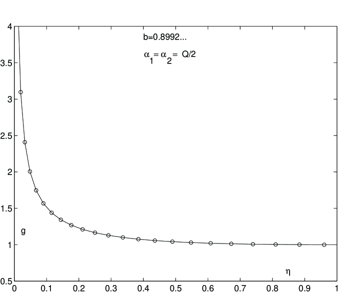
Figure 3: Normalized two-point function $g_{Q/2,Q/2}(\eta)$ evaluated as the single vacuum block (6.4) (solid line) and as the cross-channel integral (6.5) (circles).

As the first numerical example we take a quite arbitrary value $b^{2}=0.8086\ldots$ and two “puncture” operators with $\alpha_{1}=\alpha_{2}=Q/2$. In this case there are no discrete terms in the expression (6.5). The two-point function $g_{Q/2,Q/2}$ v.s. the invariant “distance” $\eta$ is plotted in fig.3. Solid line is for eq.(6.4) and circles are computed as the integral (6.5). Few numbers are presented in table 1. The first values $g^{\text{(bound)}}(\eta)$ are evaluated as the vacuum conformal block (6.4) and $g^{\text{(bulk)}}(\eta)$ stands for (6.5). We quote this table only to illustrate the numerical precision of our calculations. It should be noted that for $g^{\text{(bulk)}}(\eta)$ only the first 10 digits are correct, the errors being due to the numerical integration over $P$ in (6.5) and evaluation of the special functions entering the structure constants.

$\eta$	$g^{\text{(bound)}}(\eta)$	$g^{\text{(bulk)}}(\eta)$
0.10	1.511254162734526	1.511254162670712
0.20	1.228318394284875	1.228318394218384
0.30	1.123052815598698	1.123052815525115
0.40	1.069857238682268	1.069857238610545
0.50	1.039506854956745	1.039506854882646
0.60	1.021302866577855	1.021302866502048
0.70	1.010340291843230	1.010340291788767
0.80	1.004036952201786	1.004036952278245
0.90	1.000898855218405	1.000898855824359

Table 1: Numerical comparison of the “boundary” (6.4) and “bulk” (6.5) representations of the normalized two-point function $g_{Q/2,Q/2}(\eta)$ at $b^{2}=0.8086\ldots$

2. Vacuum $\mathbf{(m,n)=(1,2)}$. In this vacuum two boundary operators contribute with dimensions $\Delta_{1,1}=0$ and $\Delta_{1,3}=Q^{2}/4-(b^{-1}+2b)^{2}/4$. Taking again the “normalized” correlation function

$$g_{\alpha_{1}\alpha_{2}}(\eta)=\frac{\left\langle V_{\alpha_{1}}(\xi_{1})V_{\alpha_{2}}(\xi_{2})\right\rangle_{1,2}}{\left\langle V_{\alpha_{1}}(\xi_{1})\right\rangle_{1,2}\left\langle V_{\alpha_{2}}(\xi_{2})\right\rangle_{1,2}}$$ (6.6)

with respect to this vacuum, we have, instead of eq.(6.4)

$$g_{\alpha_{1}\alpha_{2}}(\eta)=(1-\eta)^{2\Delta_{1}}\times$$ (6.7)

$$\ \ \ \left[\mathcal{F}\left(\begin{array}[c]{cc}\alpha_{1}&\alpha_{2}\\ \alpha_{1}&\alpha_{2}\end{array},iQ/2,1-\eta\right)+\frac{F_{1,2}(\alpha_{1})F_{1,2}(\alpha_{2})}{U_{1,2}(-b/2)F_{1,2}(-b/2)}\mathcal{F}\left(\begin{array}[c]{cc}\alpha_{1}&\alpha_{2}\\ \alpha_{1}&\alpha_{2}\end{array},i(b+b^{-1}/2),1-\eta\right)\right]$$ (6.12)

where

$$F_{1,2}(\alpha)=\frac{B_{1,2}^{(+)}(\alpha)}{U_{1,2}(\alpha)}$$ (6.13)

as given by expression (2.17) with $(m,n)=(1,2).$ The “cross channel” representation remains the same as in eq.(6.5) with the substitution $U_{1,1}\rightarrow U_{1,2}$. In fig.4 the numerical values of (6.7) and the cross-channel integral (6.5) are compared at $b=0.7048\ldots$ and again for $\alpha_{1}=\alpha_{2}=Q/2$. Notice that in this case the two-point function $g_{\alpha_{1}\alpha_{2}}(\eta)$ is an exponentially growing function of the geodesic distance. This situation is typical for the “excited” vacua $(m,n)\neq(1,1)$ and related to the negative dimensions (5.4) of the degenerate boundary fields $\psi_{m,n}$ (at real $b$).

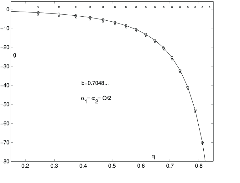
Figure 4: Boundary (6.7) (solid line) and bulk (6.5) (circles) representations of the normalized two-point function $g_{Q/2,Q/2}(\eta)$ are compared at $b=0.7048\ldots$. Small circles and crosses are respectively the contributions of the first and second terms in eq.(6.7). The two-point function is almost saturated by the $\psi_{13}$ contribution.

7 Discussion

We have demonstrated that the pseudosphere geometry provides a new physical picture of 2D quantum gravity. It is different from the compact problems and in fact much closer to standard physics in ordinary field theory (peculiarities of a field theory at constant negative curvature are discussed in [23]). However, many conceptual questions related to the suggested constructions remain open. Let us mention some of them.

• Unitary and non-unitary matter fields coupled to Liouville quantum gravity in this geometry present a separate and rather interesting problem, particularly in relation to the recent studies of AdS/CFT correspondence [24].

• Of course the closing of the bootstrap program requires construction of all bulk-boundary and boundary structure constants for all degenerate boundary fields associated with different out-vacua $(m,n)$, including the juxtaposition operators. This difficult technical task remains to be done. For “ordinary” boundary conditions in boundary LFT this program has been started in [13] (see also [21, 22, 20]).

• The most intriguing point is the nature of the “excited” vacua. As we have already mentioned, in all such vacua correlation functions typically grow exponentially with the geodesic distances. This suggests that these states can be a kind of “boundary excitations” of the corresponding boundary conformal field theory. A meaning of these quantum excitations of the (physically infinite faraway) absolute remains to be comprehended. Let us mention also that these growing correlations at large distances are dominated by non-trivial degenerate boundary operators of negative dimensions. Therefore the physical “decay property” (with which we started our arguments in sect.2) doesn’t hold literally in these excited vacua, being a formal requirement (2.12) for the contribution of the identity operator. This means that even the logic of the whole development deserves more careful examination.

Acknowledgments.

Al.Z thanks Department of Physics and Astronomy of Rutgers University, where this study has been performed. His work was also supported by EU under the contract ERBFMRX CT 960012. The work of A.Z. is supported by DOE grant DE-FG02- 96ER10919.

References

- [1] V.Kazakov. Phys.Lett., B150 (1985) 28.
- [2] V.Kazakov, I.Kostov and A.Migdal. Phys.Lett., B157 (1985) 295.
- [3] F.David. Nucl.Phys., B257 (1985) 45, 543.
- [4] J.Ambjørn, B.Durhuus and J.Fröhlich. Nucl.Phys., B257 (1985) 433.
- [5] V.Knizhnik, A.Polyakov and A.Zamolodchikov. Mod.Phys.Lett., A3 (1988) 819.
- [6] F.David. Mod.Phys.Lett., A3 (1988) 207.
- [7] J.Distler and H.Kawai. Nucl.Phys., B231 (1989) 509.
- [8] I.Klebanov. String theory in two dimensions. Lectures at ICTP Spring School on String Theory and Quantum Gravity. Trieste, April 1991, hep-th/9108019.
- [9] P.Ginsparg and G.Moore. Lectures on 2D gravity and 2D string theory. TASI summer school, 1992, hep-th/9304011.
- [10] P.Di Francesco, P.Ginsparg and J.Zinn-Justin. 2D Gravity and Random Matrices. Phys.Rep. 254 (1995) 1–133.
- [11] A.Zamolodchikov and Al.Zamolodchikov. Nucl.Phys., B477 (1996) 577.
- [12] H.Dorn and H.-J.Otto. Phys.Lett., B291 (1992) 39; Nucl.Phys., B429 (1994) 375.
- [13] V.Fateev, A.Zamolodchikov and Al.Zamolodchikov. Boundary Liouville field theory I.Boundary state and boundary two-point function. hep-th/0001012 (2000).
- [14] N.Ishibashi. Mod.Phys.Lett., A4 (1989) 251; T.Onogi and N.Ishibashi. Mod.Phys.Lett., A4 (1989) 161.
- [15] J.Teschner. On the Liouville three-point function. Phys.Lett., B362 (1995) 65.
- [16] G.-L.Gervais Comm.Math.Phys., 130 (1990) 252; E.Kremmer, G.-L.Gervais and G.-S.Roussel Comm.Math.Phys., 161 (1994) 597; G.-L.Gervais and J.Schnittger. Nucl.Phys., B431 (1994) 273.
- [17] J.Cardy. Nucl.Phys., B240[FS12] (1984) 514; Nucl.Phys., B275 (1986) 200; Nucl.Phys., B324 (1989) 581.
- [18] E.Braaten, T.Curtright, G.Ghandour and C.Thorn. Ann.Phys., 153 (1984) 147; D.Friedan, unpublished.
- [19] V.G.Kac. Infinite-dimensional Lie algebras. Prog.Math., Vol.44, Birkhäuser, Boston, 1984.
- [20] J.Teschner. Remarks on Liouville theory with boundary. Talk presented at TMR-conference “Nonperturbative Quantum Effects 2000” September 2000, hep-th/0009138.
- [21] B.Ponsot and J.Teschner. Liouville bootstrap via harmonic analysis on a noncompact quantum group. hep-th/9911110.
- [22] B.Ponsot and J.Teschner. Clebsch-Gordan and Racah-Wigner coefficients for a continuous series of representations of sl(). math.QA/0007097.
- [23] C.Callan and F.Wilczek. Nucl.Phys., B340 (1990) 366.
- [24] J.Maldacena. Adv.Theor.Math.Phys., 2 (1998) 231.
- [25] A.Strominger. Quantum Gravity and String Theory. JHEP 9901:007 (1999), hep-th/9809027; M.Spradlin, A.Strominger. Vacuum States for Black Holes. JHEP 9911:021 (1999), hep-th/9904143
- [26] E.D’Hoker, R.Jackiw. Phys.Rev. D26 (1982) 3517; Phys. Rev.Lett. 50 (1983) 1719.