Split attractor flows and the spectrum of BPS D-branes on the Quintic

Abstract:

We investigate the spectrum of type IIA BPS D-branes on the quintic from a four dimensional supergravity perspective and the associated split attractor flow picture. We obtain some very concrete properties of the (quantum corrected) spectrum, mainly based on an extensive numerical analysis, and to a lesser extent on exact results in the large radius approximation. We predict the presence and absence of some charges in the BPS spectrum in various regions of moduli space, including the precise location of the lines of marginal stability and the corresponding decay products. We explain how the generic appearance of multiple basins of attraction is due to the presence of conifold singularities and give some specific examples of this phenomenon. Some interesting space-time features of these states are also uncovered, such as a nontrivial, moduli independent lower bound on the area of the core of arbitrary BPS solutions, whether they are black holes, empty holes, or more complicated composites.

1 Introduction

Type II string theory compactified on a Calabi-Yau manifold has a rich and very nontrivial spectrum of BPS states, obtained by wrapping D-branes around various supersymmetric cycles in the compactification manifold. Over the past years, several approaches have been developed to analyze the notorious problem of existence and decay of these objects. Essentially there are two complementary viewpoints — a common theme in D-brane physics: the microscopic D-brane picture and the macroscopic supergravity description. The former has been studied by far the most, as it provides a direct, powerful and extensive framework, firmly rooted in geometry and string theory. A partial list of references is [1, 2, 3, 4, 5, 6, 7, 8, 9, 10, 11, 12, 13, 14, 15, 16, 17, 18, 19, 20, 21, 22]. The alternative approach, based on the four dimensional low energy effective ${\mathcal{N}}=2$ supergravity theory, has received considerably less attention, in part because at first sight this effective theory seemed much too simple to be able to capture the intricacies of the D-brane spectrum. To a large extent, this is true, though a number of intriguing surprises were uncovered, starting with the work of [23], where BPS black hole solutions and the associated attractor mechanism of [24] were studied, and it was found that existence of these solutions for given charge and moduli is quite nontrivial and linked to some deep results in microscopic D-brane physics and arithmetic, suggesting a correspondence between existence of BPS black hole solutions and BPS states in the full string theory. This conjecture turned out to fail in a rather mysterious way in a number of cases [3, 25], but it was soon realized how to fix this: more general, non-static (but stationary) multicenter solutions have to be considered, and corresponding to those, more general attractor flows, the so-called split attractor flows [25, 28]. Thus, an unexpectedly rich structure of solutions emerged, providing a low energy picture of many features of the BPS spectrum, including bound states, intrinsic angular momentum, decay at marginal stability, and a number of stability criteria tantalizingly similar to those obtained from microscopic brane physics and pure mathematics. Moreover, further evidence was found for the correspondence between (split) attractor flows and stringy BPS states, which might even extend beyond the supergravity regime.

In this paper, we further explore this approach, focusing on the well-known and widely studied example of type IIA theory compactified on the quintic Calabi-Yau (or IIB on its mirror) [29, 2], mainly on the basis of an extensive numerical analysis. We give various examples of the sort of results that can be obtained using the split flow picture, predict presence and absence of some charges in various regions of moduli space (including precise lines of marginal stability and corresponding decay products), elucidate the appearance of multiple basins of attraction and give some examples of this phenomenon, compare our numerical results for the fully instanton-corrected theory with analytical results in the large radius approximation, obtain an interesting lower bound on the area of all BPS objects in the supergravity theory, and briefly discuss some extentions to non-BPS states and the zoo of near horizon split flows. Our main conclusion is that surprisingly much can be learned from the supergravity picture, in a very concrete way, though fundamental insight in the spectrum is still more likely to come from the microscopic picture.

The outline of the paper is as follows. In section 2, we review the construction of stationary BPS solutions of four dimensional ${\mathcal{N}}=2$ supergravity (including the enhançon [30] related empty hole) and their relation to split flows, and give some comments on the validity of the four dimensional supergravity approximation. In section 3, we explain how one can obtain (split) attractor flow spectra, based on a number of existence criteria, and we show how the presence of singularities generically induces multiple basins of attraction, and how the split flow picture avoids a clash with microscopic entropy considerations. Section 4 reviews the essentials of compactification on the quintic. In section 5, we outline the practical strategies we followed for computing attractor flows, which we apply in section 6 to a broad analysis of the quintic. More precisely, in section 6.2, some features of the single flow spectrum around the Gepner point are analyzed, including a screening of a large number of candidate BPS states, supporting physical expectations of discreteness of the BPS spectrum. In 6.3, we give an example of a charge that exists as a BPS black hole at large radius, but decays when the moduli are varied towards the Gepner point, where it is absent from the spectrum, providing a nice qualitative distinction between large and small radius physics. Section 6.4 gives an example of an interesting bound state of two black holes at large radius that does not exist as a single black hole [but does have yet another composite realization, without (regular, four dimensional) black hole constituents] and decays on its way to the Gepner point. Section 6.5 gives an example of the mulitple basin phenomenon. In 6.6 we have a look at exact results in the large radius approximation, and compare this with numerical results for the interesting example of D6-D2 states. A puzzle related to the stability of solutions in the presence of conifold singularities is raised in section 6.7, but not conclusively resolved, though we suggest some possible ways out. In 6.8 we go back to spacetime properties of the solutions, and find that they all satisfy a certain area bound, which we explicitly compute. Finally, in 6.9, we briefly comment on multicenter configurations in the near horizon region of a black hole, and find that there are many more possibilities here than in asymptotically flat space. We end with our conclusions and some discussion in section 7.

2 BPS solutions of 4d N=2 supergravity and split attractor flows

2.1 Special geometry of type IIB Calabi-Yau compactifications

For concreteness, we will assume that the four dimensional ${\mathcal{N}}=2$ supergravity theory is obtained from a compactification of type IIB string theory on a Calabi-Yau 3-fold $X$. This theory has $n_{v}=h^{1,2}(X)$ massless abelian vector multiplets and $n_{h}=h^{1,1}(X)+1$ massless hypermultiplets. The hypermultiplet fields will play no role here and are set to constant values.

The vector multiplet scalars are given by the complex structure moduli of $X$, and the lattice of electric and magnetic charges is identified with $H^{3}(X,\mathbb{Z})$, the lattice of integral harmonic $3$-forms on $X$: after a choice of symplectic basis ${\alpha^{I},\beta_{I}}$ of $H^{3}(X,\mathbb{Z})$, a D3-brane wrapped around a cycle Poincaré dual to $\Gamma\in H^{3}(X,\mathbb{Z})$ has electric and magnetic charges equal to its components with respect to this basis.

The geometry of the vector multiplet moduli space, parametrized by $n_{v}$ coordinates $z^{a}$, is special Kähler [31]. The (positive definite) metric

$$g_{a\bar{b}}=\partial_{a}\bar{\partial}_{\bar{b}}{\mathcal{K}}$$ (1)

is derived from the Kähler potential

$${\mathcal{K}}=-\ln\left(i\int_{X}\Omega\wedge\bar{\Omega}\right),$$ (2)

where $\Omega$ is the holomorphic $3$-form on $X$, depending holomorphically on the complex structure moduli. It is convenient to introduce also the normalized 3-form

$$\tilde{\Omega}\equiv e^{{\mathcal{K}}/2}\,\Omega\,.$$ (3)

The “central charge” of $\Gamma\in H^{3}(X,\mathbb{Z})$ is given by

$$Z(\Gamma)\equiv\int_{X}\Gamma\wedge\tilde{\Omega}\equiv\int_{\Gamma}\tilde{\Omega}\,,$$ (4)

where we denoted, by slight abuse of notation, the cycle Poincaré dual to $\Gamma$ by the same symbol $\Gamma$. Note that $Z(\Gamma)$ has a nonholomorphic dependence on the moduli through the Kähler potential.

The (antisymmetric, topological, moduli independent) intersection product is defined as:

$$\langle\Gamma_{1},\Gamma_{2}\rangle=\int_{X}\Gamma_{1}\wedge\Gamma_{2}=\int_{\Gamma_{1}}\Gamma_{2}=\#(\Gamma_{1}\cap\Gamma_{2})\,.$$ (5)

With this notation, we have for a symplectic basis $\{\alpha^{I},\beta_{I}\}$ by definition $\langle\alpha^{I},\beta_{J}\rangle=\delta^{I}_{J}$, so for $\Gamma_{i}=q_{i}^{I}\beta_{I}-p_{i,I}\alpha^{I}$, we have $\langle\Gamma_{1},\Gamma_{2}\rangle=q_{1}^{I}p_{2,I}-p_{1,I}q_{2}^{I}$. This is nothing but the Dirac-Schwinger-Zwanziger symplectic inner product on the electric/magnetic charges. Integrality of this product is equivalent to Dirac charge quantization.

2.2 BPS configurations

2.2.1 Single charge type: single flows

Static, spherically symmetric BPS configurations [24, 32, 33, 34] with charge $\Gamma\in H^{3}(X,\mathbb{Z})$ at the origin of space have a spacetime metric of the form

$$ds^{2}=-e^{2U}dt^{2}+e^{-2U}dx^{i}dx^{i}\,,$$ (6)

with $U$ a function of the radial coordinate distance $r=|\bf{x}|$, or equivalently of the inverse radial coordinate $\tau=1/r$. We will take space to be asymptotically flat, with $U_{\tau=0}=0$. The BPS equations of motion for $U(\tau)$ and the moduli $z^{a}(\tau)$ are:

$$\partial_{\tau}U = -e^{U}|Z|\,,$$ (7)

$$\partial_{\tau}z^{a} = -2e^{U}g^{a\bar{b}}\,\bar{\partial}_{\bar{b}}|Z|\,,$$ (8)

where $Z=Z(\Gamma)$ is as in (4) and $g_{a\bar{b}}$ as in (1). The electromagnetic field is given algebraically and in closed form in terms of the solutions of these flow equations, but we will not need the explicit expression here.

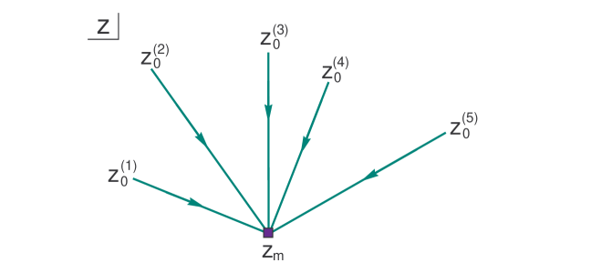
Figure 1: Sketch of some single charge attractor flows in moduli space, for different values $z_{0}^{(i)}$ of the moduli at spatial infinity. The attractor point is indicated by $z_{m}$.

An alternative form of the equations is:

$$2\,\partial_{\tau}[e^{-U}\mathop{\rm Im}\nolimits(e^{-i\alpha}\tilde{\Omega})]=-\Gamma\,,$$ (9)

where $\alpha=\arg Z$, which can be shown to be the phase of the conserved supersymmetry [23]. Note that this nice compact equation actually has $2n_{v}+2$ real components, corresponding to taking intersection products with the $2n_{v}+2$ elements of a basis $\{C_{L}\}_{L}$ of $H^{3}(X,\mathbb{Z})$:

$$2\,\partial_{\tau}[e^{-U}\mathop{\rm Im}\nolimits(e^{-i\alpha}Z(C_{L}))]=-\langle C_{L},\Gamma\rangle\,,$$ (10)

One component is redundant, since taking the intersection product of (9) with $\Gamma$ itself produces trivially $0=0$. This leaves $2n_{v}+1$ independent equations, matching the number of real variables $\{U,\mathop{\rm Re}\nolimits z^{a},\mathop{\rm Im}\nolimits z^{a}\}$.

Since the right hand side of (10) consists of $\tau$-independent integer charges, (9) integrates to

$$2\,e^{-U}\mathop{\rm Im}\nolimits[e^{-i\alpha}\tilde{\Omega}]=-\Gamma\,\tau+2\mathop{\rm Im}\nolimits[e^{-i\alpha}\tilde{\Omega}]_{\tau=0}.$$ (11)

This solves in principle the equations of motion. Of course, finding the explicit flows in moduli space from (11) requires inversion of the periods to the moduli, which in general is not feasible analytically. For this paper, which studies the case of the quintic Calabi-Yau for arbitrary values of the moduli, we developed some numerical approaches to tackle this problem.

Generalization to the multicenter BPS configurations with identical charges $\Gamma$ at locations ${\bf x}_{p}$ (arbitrary and possibly coinciding) is straightforward: one just replaces $\tau=1/|{\bf x}|$ by $\sum_{p}1/|{\bf x}-{\bf x}_{p}|$. Thus, the flow in moduli space will remain the same, only its spacetime parametrization changes.

It was observed in [23] that the attractor flows in moduli space given by the BPS equations do not always exist. While solutions to (7)-(8) generically do exist for a finite range of $\tau$ (starting from spatial infinity $\tau=0$), they can break down before $\tau=\infty$ is reached. This can be seen as follows (see e.g. [23, 25, 28] for more details). The BPS equations imply that, away from a singular point or a critical point of $|Z|$,

$$\partial_{\tau}|Z|=-4\,e^{U}g^{a\bar{b}}\,\partial_{a}|Z|\,\bar{\partial}_{\bar{b}}|Z|<0\,,$$ (12)

so along a flow, $|Z|$ is a decreasing function, converging to a local minimum, the so-called attractor point (see fig. 1). Three cases are distinguished [23], depending on the value $|Z_{m}|$ and the position $z_{m}$ of this minimum in moduli space:

1. $|Z_{m}|\neq 0$: the flow exists all the way up to $\tau=\infty$ and the solution exists as a regular BPS black hole, with $\mathrm{AdS}_{2}\times S^{2}$ near horizon geometry and horizon area $A=4\pi|Z_{m}|^{2}$. Note that the horizon moduli $z_{m}$ are generically invariant under continuous variations of the moduli at spatial infinity. The moduli at the horizon satisfy the so-called attractor equation:

   $$2\mathop{\rm Im}\nolimits(\bar{Z}\tilde{\Omega})=-\Gamma$$ (13)

2. $|Z_{m}|=0$ and $z_{m}$ is a regular point of moduli space: the flow breaks down at finite $\tau$, where the zero of $Z$ is reached, since at this point, the inequality in (12) does not make sense. So no BPS solutions exists in this case. This is compatible with physical expectations, since the existence of a BPS state with the given charge in a vacuum where $Z$ vanishes would imply the existence of a massless particle there, which in turn is expected to create a singularity in moduli space at the zero, contradicting the assumption of regularity of that point. Or, from a geometric point of view: if a supersymmetric wrapped brane exists at the zero, its volume is zero, so we must have a vanishing cycle in the Calabi-Yau, leading to a singularity in moduli space.

3. $|Z_{m}|=0$ and $z_{m}$ is a singular (or boundary) point in moduli space: in this case the arguments of (2) for nonexistence fail, and indeed well-behaved solutions may exist, like for example the repulson-resolving empty hole solutions of [25], arising from flows attracted to a conifold locus. These correspond to the famous states of [35], resolving the conifold singularity in string theory.

2.2.2 Mutually nonlocal charges: split flows

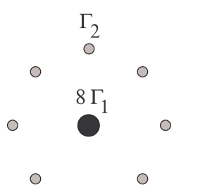
Figure 2: Example of a $(\Gamma_{1},\Gamma_{2})$-multicenter configuration with total charge $8\,\Gamma_{1}+7\,\Gamma_{2}$.

It was shown in [25] that for some examples of BPS states, established by CFT methods to exist in the full string theory, the corresponding flows in moduli space break down at a regular zero, making it is necessary to consider more general BPS solutions, in particular multicenter solutions with mutually nonlocal charges (fig. 2). Unfortunately, the BPS equations [26, 25, 27] — though formally quite similar to the spherically symmetric equations — become substantially more complicated to solve in this case. This is partly due to the fact that with mutually nonlocal charges, solutions are in general no longer static, as they acquire an intrinsic angular momentum (even though the charge positions are time independent), a fact that is well known from ordinary Maxwell electrodynamics with magnetically and electrically charged particles.

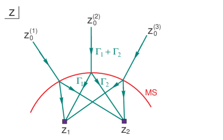
Figure 3: Sketch of some split flows for different moduli values $z_{0}^{(i)}$ at spatial infinity, in the case of two different constituent charges $\Gamma_{1}$ and $\Gamma_{2}$, with attractor points $z_{1}$ resp. $z_{2}$. The line labeled “MS” is (part of) the $(\Gamma_{1},\Gamma_{2})$-marginal stability line.

The metric in this case is given by an expression of the form

$$ds^{2}=-e^{2U}\left(dt+\omega_{i}\,dx^{i}\right)^{2}+e^{-2U}dx^{i}dx^{i}\,,$$ (14)

and (11) elegantly generalizes to

$$2\,e^{-U}\mathop{\rm Im}\nolimits[e^{-i\alpha}\tilde{\Omega}] = H\,,$$ (15)

$$\boldsymbol{*}d\omega = \langle dH,H\rangle\,,$$ (16)

with $H({\bf x})$ an $H^{3}(X)$-valued harmonic function (on flat coordinate space $\mathbb{R}^{3}$), and $\boldsymbol{*}$ the flat Hodge star operator on $\mathbb{R}^{3}$. For $N$ charges $\Gamma_{p}$ located at coordinates ${\bf x}_{p}$, $p=1,\ldots,N$, in asymptotically flat space, one has:

$$H=-\sum_{p=1}^{N}\Gamma_{p}\,\tau_{p}\,\,+\,2\mathop{\rm Im}\nolimits[e^{-i\alpha}\tilde{\Omega}]_{r=\infty}\,,$$ (17)

with $\tau_{p}=1/|{\bf x}-{\bf x}_{p}|$.

It was shown in [25] and in more detail in [28], that such multicenter BPS configurations do indeed exist, and the existence question in a particular situation essentially boils down to existence of a corresponding split attractor flow, instead of the single flow associated to the single charge case (see fig. 3). The endpoints of the attractor flow branches are the attractor points of the different charges $\Gamma_{p}$ ($p=1,\ldots,N$) involved, which are located at equilibrium positions ${\bf x}_{p}$ subject to the constraint

$$\sum_{q=1}^{N}\frac{\langle\Gamma_{p},\Gamma_{q}\rangle}{|{\bf x}_{p}-{\bf x}_{q}|}=2\,\mathop{\rm Im}\nolimits[e^{-i\alpha}Z(\Gamma_{p})]_{r=\infty},$$ (18)

with $\alpha=\arg Z(\sum_{p}\Gamma_{p})$. For such a multicenter solution, the image of the moduli fields in moduli space will look like a “fattened” version of the split flow (fig. 4). In analogy with the picture arising in the brane worldvolume description of low energy quantum field theory, one could imagine space as a “3-brane” embedded in moduli space through the moduli fields $z^{a}({\bf x})$, with the positions of the charges mapped to their respective attractor points in moduli space.

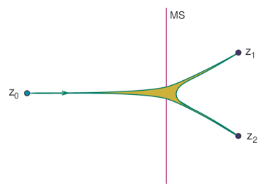
Figure 4: Sketch of the image of $z({\bf x})$ in moduli space for a $(\Gamma_{1},\Gamma_{2})$-multicenter solution, with attractor points $z_{1}$ resp. $z_{2}$, and modulus at spatial infinity $z_{0}$. The line labeled “MS” is a $(\Gamma_{1},\Gamma_{2})$-marginal stability line.

It turns out that the splitting points of the flows have to lie on a surface of marginal stability in moduli space [25]; more precisely, a $\Gamma$-flow can only split in a $\Gamma_{1}$- and a $\Gamma_{2}$-flow at a surface of $(\Gamma_{1},\Gamma_{2})$-marginal stability, that is, where $\arg Z(\Gamma_{1})=\arg Z(\Gamma_{2})$.

We will primarily consider situations with only two different charges $\Gamma_{1}$ and $\Gamma_{2}$ (located in an arbitrary number of centers), for example a core at the origin of space with $N$ charges $\Gamma_{1}$ surrounded by a homogeneous “cloud” of $N$ charges $\Gamma_{2}$, constrained by (18) to lie on a sphere of coordinate radius

$$r_{\mathrm{ms}}=N\,\frac{1}{2}\langle\Gamma_{1},\Gamma_{2}\rangle\left.\frac{|Z_{1}+Z_{2}|}{\mathop{\rm Im}\nolimits(\bar{Z_{2}}Z_{1})}\right|_{r=\infty}\,.$$ (19)

Note that when the moduli at infinity approach the surface of marginal stability, the right hand side of (19) diverges, yielding a smooth decay of the BPS bound state into its constituents, as could be physically expected. More complicated split flows can also be considered, with branches splitting several times. However, many of the features of those more complex configurations can be understood by iteration of what is known about split flows with just one split point.

Thus, the main point of this section is that the supergravity BPS spectrum is essentially given by the spectrum of attractor flows on moduli space, including split flows. This will be the basic starting point for our exploration of the BPS spectrum of type IIA string theory compactified on the quintic (or its IIB mirror).

There is one comment to be made here though: composite configurations involving charges that give rise to empty hole solutions (when those charges are isolated), such as particles obtained by wrapping a D3-brane around a vanishing conifold cycle, seem to be somewhat more subtle than their siblings consisting exclusively of regular black hole components. In particular, no explicit truly solitonic construction of the former was given in [28], only an idealized spherical shell configuration, which requires the addition of a shell of smeared out wrapped branes with nonvanishing bare mass (whose existence, strictly speaking, cannot directly be predicted by the supergravity theory alone). Probably such a construction can be given with appropriately delocalized charge located on a “superconducting” surface, but this might put additional constraints on the existence of the solution, beyond those implied by the mere existence of a split flow. We hope to address this issue elsewhere.

2.3 Validity of the four dimensional supergravity approximation

Denote the four dimensional Newton constant by $G_{N}$. In the IIB theory, $G_{N}$ is related to the string coupling constant $g$, the string scale $l_{s}$ and the volume $V_{X}$ of the Calabi-Yau manifold by $G_{N}\sim g^{2}l_{s}^{8}/V_{X}$. The four dimensional effective supergravity description of the IIB string theory can only be trusted if the characteristic distance scale $L\sim N\sqrt{G_{N}}$ of the charge $N$ solution under consideration is much larger than the string scale $l_{s}$, the inverse mass $m^{-1}=|Z|^{-1}\sqrt{G_{N}}$ of the lightest BPS particle obtained by wrapping a D3-brane, and the “size” $R_{X}$ of the internal Calabi-Yau manifold $X$. With “size” we mean any relevant linear dimension of $X$; hence $R_{X}$ is in part dependent on both the complex and Kähler structure moduli. These dimensions have to be sufficiently small to justify the four dimensional approximation.

Note that the second and third conditions are dependent on the complex structure moduli, so for some solutions, it might be impossible to satisfy this condition everywhere in space, since the moduli could be driven to values where $|Z|\to 0$ or $R_{X}\to\infty$. The former is the case for example for the empty hole solutions discussed above. So in principle, we should include an additional light field in the Lagrangian near the core of such solutions. At large $N$, this presumably would only have the effect of somewhat smoothing out the solution. It would be interesting to study this in more detail.

The complication $R_{X}\to\infty$ occurs typically for charges of $D0-D2$ type in the IIA picture: the moduli are driven to large complex structure, where the dimensions of the IIB Calabi-Yau transverse to the corresponding IIB D3-branes become infinitely large.

The physical 4d low energy arguments based on supergravity considerations we present in this paper are only valid if the above conditions are met. However, some arguments rely only on energy conservation considerations starting from the BPS formula, and since this formula is protected by supersymmetry, those arguments should also hold outside the supergravity regime. Also, the conjectured correspondence between BPS states and (split) attractor flows itself might extend beyond the supergravity regime. We will refer to this as the strong version of the conjecture.

3 Attractor flow spectra

3.1 Existence criteria for split flows

As illustrated in fig. 3, in order for a split flow $\Gamma\to(\Gamma_{1},\Gamma_{2})$ to exist, the following two conditions have to be satisfied:

1. The single flow corresponding to the total charge $\Gamma=\Gamma_{1}+\Gamma_{2}$, starting at the value of the moduli at spatial infinity, has to cross a surface of $(\Gamma_{1},\Gamma_{2})$-marginal stability.

2. Starting from this crossing point, both the $\Gamma_{1}$-flow and the $\Gamma_{2}$-flow should exist.

For more complicated split flows (with more split points), these condition have to be iterated.

A simple necessary condition for condition (1) can be derived from the integrated BPS equation (11). Taking the intersection product of this equation with $\Gamma_{1}$ gives

$$2e^{-U}\mathop{\rm Im}\nolimits(e^{-i\alpha}Z_{1})=-\langle\Gamma_{1},\Gamma\rangle\,\tau+2\,\mathop{\rm Im}\nolimits(e^{-i\alpha}Z_{1})_{\tau=0}\,.$$ (20)

When $Z_{1}$ and $Z_{2}$ are parallel (or anti-parallel), the left hand side vanishes. On the other hand, since the right hand side is linear in $\tau$, and $\tau$ has to be positive, this can at most happen once along the flow, namely iff

$$r_{\mathrm{ms}}\equiv 1/\tau_{\mathrm{ms}}\equiv\frac{1}{2}\langle\Gamma_{1},\Gamma_{2}\rangle\left.\frac{|Z_{1}+Z_{2}|}{\mathop{\rm Im}\nolimits(Z_{1}\bar{Z_{2}})}\right|_{r=\infty}>0\,,$$ (21)

and the flow does not hit a zero before $Z_{1}$ and $Z_{2}$ become (anti-)parallel (when the full flow has a regular attractor point, the latter is of course automatically satisfied). Furthermore, only the case where $Z_{1}$ and $Z_{2}$ become parallel (so $|Z|>|Z_{1}|$ and $|Z|>|Z_{2}|$) rather than anti-parallel (so $|Z_{1}|>|Z|$ or $|Z_{2}|>|Z|$) gives rise to a split flow. So (21) is a necessary but not sufficient condition for (1) to hold.

A few simple observations can be made at this point:

• From the discussion of equation (19) in the previous section, it follows that this existence condition for a split flow is just the statement that the radius of separation between two differently charged source centers is positive. When the moduli at infinity approach the surface of marginal stability, this radius diverges, and the configuration decays smoothly.

• Generically, $\Gamma_{1}$ and $\Gamma_{2}$ must be mutually nonlocal ($\langle\Gamma_{1},\Gamma_{2}\rangle\neq 0$) to have a split flow (and hence a stationary BPS multicenter solution). A degenerate exception occurs for mutually local charges when the moduli at spatial infinity are already at a surface of marginal stability: then the “incoming” branch of the split flow vanishes, and a multicenter solution exists for arbitrary positions of the centers.

• Since the right-hand side of (20) can only vanish for one value of $\tau$, the phases $\alpha_{i}$ of the central charges $Z_{i}$ will satisfy $|\alpha_{1}-\alpha_{2}|<\pi$ (at least if we put $\alpha_{1}=\alpha_{2}$ at marginal stability, as opposed to $\alpha_{1}=\alpha_{2}+2n\pi$), even though separately, they do not have to stay in the $(-\pi,\pi)$-interval.

• This also implies that for mutually nonlocal charges, we can rewrite (21) as

  $$\langle\Gamma_{1},\Gamma_{2}\rangle\,(\alpha_{1}-\alpha_{2})>0\,,$$ (22)

  where $\alpha_{i}=\arg Z(\Gamma_{i})_{r=\infty}$. This is precisely the stability condition for “bound states” of special lagrangian 3-cycles found in a purely geometrical setting by Joyce [19] in the case where $\Gamma_{1}$ and $\Gamma_{2}$ are special Lagrangian 3-spheres, and for values of the moduli sufficiently close to marginal stability.

The above stability criterion is also quite similar to Douglas’ triangle stability criterion [14], roughly as follows. Consider three BPS charges $\bar{A}$, $B$ and $C$, with $C=\bar{A}+B$ and $\langle\bar{A},B\rangle>0$ (so $\langle B,C\rangle<0$ and $\langle C,\bar{A}\rangle<0$). Identify Douglas’ “morphism grade” between $P,Q\in\{A,B,C\}$ with $\phi_{PQ}\equiv(\alpha_{Q}-\alpha_{P})/\pi$, where $\alpha_{P}$ ($\alpha_{Q}$) is the phase of $Z_{P}$ ($Z_{Q}$) and $\alpha_{\bar{A}}\equiv\alpha_{A}+\pi$. Obviously, $\phi_{AB}+\phi_{BC}+\phi_{CA}=1$. By suitable labeling, we can assume $\langle\Gamma_{1},\Gamma_{2}\rangle>0$ for the composite state considered above, so we can take $\bar{A}=\Gamma_{1}$, $B=\Gamma_{2}$ and $C=\Gamma$. The above stability criterion for the composite state can now be rephrased as $0<\phi_{AB},\phi_{BC},\phi_{CA}<1$, that is, in the terminology of [14], $(A,B,C)$ forms a “stable triangle”.

Though there is an obvious similarity, this connection needs further clarification. In particular, the role of morphism grades outside the interval $(-1,1)$ is obscure in the supergravity context at this point (see however section 6.7).

3.2 Building the spectrum

How can we determine whether there exists a (split) flow or not for a given charge $\Gamma$ and vacuum moduli $z_{0}$?

To find out if a single flow exists is no problem: basically, one just has to check whether or not the central charge is zero at the attractor point, as explained in section 2.2.1. So one can in principle determine algorithmically the single flow spectrum at any point $z_{0}$ in moduli space.

The split flow spectrum is more difficult to obtain. Let us first consider the simplest case, split flows with only one splitting point, say $\Gamma\to\Gamma_{1}+\Gamma_{2}$. At first sight, it might seem that an infinite number of candidate constituents ($\Gamma_{1}$,$\Gamma_{2}$) has to be considered. However, the situation is not that bad, at least if the mass spectrum of single flows is discrete, does not have accumulation points, and is roughly proportional to charge. This is what one would expect physically, and we give an argument for this property of the spectrum in appendix A, based on an interesting link with the multi-pronged string picture of quantum field theory BPS states. Then indeed, because $|Z(\Gamma)|$ is decreasing along the $\Gamma$-flow, and at the split point we have $|Z(\Gamma)|=|Z(\Gamma_{1})|+|Z(\Gamma_{2})|$, we only need to consider pairs $(\Gamma_{1},\Gamma_{2})$ in the single flow spectrum with mass less than $|Z(\Gamma)|_{\tau=0}$. Therefore, if the single flow spectrum has indeed the above properties, we only need to consider a finite number of cases.

In practice, to figure out precisely at which charge numbers one can stop checking candidates, is of course a nontrivial problem on its own. Nevertheless, in some cases it can be carried out without too much difficulty, as we will illustrate in section 6.

3.3 Monodromies and multiple basins of attraction

In [23], it was observed that a charge $\Gamma$ does not necessarily have the same attractor point for all possible values of the vacuum moduli: the moduli space (or more precisely its covering space) can be divided in several different “basins of attraction”. Therefore, the corresponding black hole horizon area and the BH-entropy are not just a function of the charge, but also of the basin to which the vacuum moduli belong. This data was called the “area code” in [23]. This nonuniqueness might seem somewhat puzzling, especially in the light of statistical entropy calculations using D-branes. Also, what happens to the supergravity solution when one moves from one basin to the other seems rather obscure: do we get a catastrophe, a jump, a discontinuity?

We will clarify these issues here, arriving once again at a beautiful picture of how string theory resolves naive disasters.

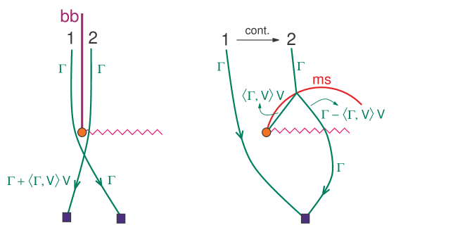
Figure 5: Left: A conifold singularity (the red dot), with vanishing cycle $V$, as source for different basins of attraction. The flows to the left and the right of the basin boundary (labeled “bb”) have different attractor points, due to the monodromy. The horizontal wiggly line is a cut. Right: This is what really happens when a flow is continuously moved from 1 to 2: it transforms into a split flow with the new branch ending on the singularity. The red line labeled “ms” is the corresponding $(\langle\Gamma,V\rangle V,\Gamma-\langle\Gamma,V\rangle V)$-marginal stability line.

The key observation is that jumps in the basin of attraction are caused by the presence of singularities at finite distance in moduli space, such as the conifold point for the quintic. Suppose we have a singularity locus $z_{s}$ associated to a vanishing cycle $V$, so that the monodromy about this singularity is given by

$$\Gamma\to\Gamma+\langle\Gamma,V\rangle\,V\,.$$ (23)

Consider, as shown in fig. 5, a $\Gamma$-flow that passes just to the left of $z_{s}$, with $\langle\Gamma,V\rangle\neq 0$. Now move the starting point of the flow to the right, as if we were trying to “pull” the flow through the singularity. We will not succeed to do this smoothly, because of the monodromy: a flow starting off with charge $\Gamma$ and passing just to the right of $z_{s}$ can no longer be assigned charge $\Gamma$ at points beyond the singularity; instead, we should assign it charge $\Gamma^{\prime}=\Gamma+\langle\Gamma,V\rangle\,V$. One way to understand this is that the second flow necessarily crosses the cut starting at $z_{s}$ (we assumed implicitly that the first one does not; this is of course purely conventional). This means that this flow will no longer converge to a $\Gamma$-attractor point, but rather to a $\Gamma^{\prime}$-attractor point, which in general will be different from the original one, with a different value for $|Z|_{\mathrm{min}}$, possibly even a regular zero (in that case, no single center BPS solution exists anymore). Thus we get two basins of attraction, with boundary formed by the “critical” flow, i.e. the $\Gamma$-flow hitting the singularity $z_{s}$.

Does this mean the solution and its intrinsic properties such as entropy jump discontinuously when we vary the vacuum moduli in this way, possibly even kicking the state out of the spectrum (without obvious decay products)? The answer is no. As explained in more detail in [25], what really happens is that, upon moving the flow through the singularity, $n=\langle V,\Gamma\rangle$ units of $V$-charge are created at the locus in space where the moduli acquire the singular value $z_{s}$.

This is consistent with energy conservation, because at this locus, $V$ particles are massles. It is also consistent with charge conservation, because of the subtleties associated to the monodromy. In the case of the example at hand, when one continues varying the vacuum moduli, the newly born $V$-particles will acquire mass, and a full-fledged multicenter solution (of the type described in the previous section) emerges. The black hole core remains unchanged however, and all fields change smoothly during the transition.

In the split flow picture (see also fig. 5), what happens is that the attractor flow gets a new branch, of charge $nV$, terminating on the singularity locus (corresponding to a (multi) empty hole constituent). Note that because $Z(V)$ is zero at $z_{s}$, there will always be a surface (or line) of $(V,\Gamma)$ marginal stability starting at $z_{s}$, as is needed for the split flow to exist. Furthermore, if one tried to continue circling around the singularity, one would unavoidably cross this surface of marginal stability, and a decay would result. Thus, mondromies about singularities of this kind will always induce decay of the configuration (if one is sufficiently near the singularity). This does not mean that this charges disappears from the spectrum: other BPS configurations with this charge can still exist.

Similar things could happen near different kinds of singularities (not of “conifold”-type), though not necessarily so. For instance, circling around the large complex structure point of the quintic with a generic flow will not do anything spectacular, essentially because the LCS point is at infinite distance in the moduli space, making it impossible for the flow to “cross”. Instead, it will just get wrapped around it.

The phenomena described in this section are completely analogous to what happens in the transition from simple to three-pronged strings in the description of QFT BPS states [36, 37], though it arises here from a quite different starting point. The effective string action of appendix A makes this analogy quite precise, allowing us to carry over many of the insights obtained in that context.

4 Type IIA string theory on the Quintic and its IIB mirror

In the remainder of this paper, we will apply the above general considerations to type IIA string theory compactified on the quintic Calabi-Yau $X$, or equivalently type IIB compactified on its mirror $Y$.

The quintic has $h^{2,1}(X)=101$ and $h^{1,1}(X)=1$. Consequently, the four dimensional low energy supergravity theory of a IIA compactification on $X$ has one vector multiplet, where the complex scalar corresponds to the complexified Kähler modulus of $X$. Its mirror manifold $Y$ has $h^{2,1}(Y)=1$ and $h^{1,1}(Y)=101$, and the complex scalar of the vector multiplet in the IIB low energy theory corresponds to the complex structure modulus of $Y$. The manifold $Y$ is defined by a single homogeneous equation of Fermat type:

$${\sum_{i=1}}^{5}{x_{i}^{5}}-5\,\psi\,{x_{1}x_{2}x_{3}x_{4}x_{5}}=0$$ (1)

with $x_{i}$ homogeneous coordinates on ${\mathbb{C}}P^{4}$ and a single complex parameter $\psi$, the complex structure modulus. More precisely, $Y$ is the quotient of this algebraic variety by the identifications $x_{i}\simeq\omega^{k_{i}}x_{i}$, with $\omega=e^{2\pi i/5}$ and the $k_{i}\in\mathbb{Z}$ satisfying $\sum_{i}k_{i}=0$. Note also that the $\psi$-plane is actually a 5-fold covering of moduli space, since $\psi$ and $\omega\psi$ yield isomorphic spaces through the isomorphism $x_{1}\to\omega x_{1}$.

4.1 Quantum Volumes and Meijer Functions

For the sake of future generalizations, we will start by formulating our analysis of the quintic in the rather general framework of [39] and the work upon which it is drawn. Readers desiring a more explicit treatment of these matters are encouraged to consult the reference given above.

Define the quantum volume [40] of a holomorphic even dimensional cycle in an algebraic variety with trivial anticanonical bundle to be equal to the quantum corrected mass of the (IIA) BPS saturated D-brane state wrapping it; this is equal to the classical mass of its mirror 3-cycle. In the large radius limit, this prescription agrees with our naive notion of volume, but as we move into the quantum regime, corrections arise which severely alter the behavior of these volumes as functions of the moduli, away from what one would expect. In this manner, we may obtain a quantum mechanically exact expression for the volume of a given even dimensional holomorphic cycle $\gamma$ in a variety $X$ with trivial anti-canonical bundle, in terms of the normalized period (4) of its mirror 3-cycle $\Gamma$:

$$V(\gamma)=M(\gamma)=|Z(\Gamma)|=\frac{|\int_{\Gamma}{\Omega(z)}|}{(\int_{Y}{i\,\Omega(z)\wedge{\overline{\Omega}(z)}})^{1/2}}~{}~{}=\frac{|q^{i}\int_{\Gamma_{i}}{\Omega}|}{(\int_{Y}{i\,\Omega(z)\wedge{\overline{\Omega}(z)}})^{1/2}}~{}~{}.$$ (2)

In the above, $\{\Gamma_{i}\}_{i}$, $i=1,\ldots,2h^{2,1}(Y)+2$, is an integral basis of $H_{3}(Y)$, $\Omega(z)$ is the holomorphic three-form, written with explicit dependence on the moduli $z$, $q^{i}$ are the integral charges of the cycle with respect to the $\Gamma_{i}$, and $\int_{\Gamma_{i}}{\Omega(z)}$ are the periods of the holomorphic three-form.

In a model where $h^{1,1}(X)=1$, such as the quintic, there is only one modulus, and we may identify a point $z=0$ with the so called large complex structure limit, i.e. the complex structure for the mirror variety $Y$ which is mirror to the large volume limit of $X$. In this class of examples, holomorphic cycles of real dimension $2j$ on $X$ are mirror to three-cycles on $Y$ whose periods have leading ${\rm log}^{j}z$ behavior near $z=0$. Thus, finding a complete set of periods of $\Omega(z)$ and classifying their leading logarithmic behavior gives us a means of identifying the dimension of their even-cycle counterpart on $X$. In this context, when we speak about a cycle on $X$ of real dimension $2j$, we refer to a cycle on $X$ with $2j$ being the maximal dimensional component, but with the identity of the various lower dimensional “dissolved” cycles left unspecified. More input is needed to identify the latter.

The technology of Meijer periods [41, 42] allows us to write down a basis of solutions to the Picard-Fuchs equation associated to a given variety $Y$, which is indexed by the leading logarithmic behavior of each solution. In particular, we are able to find a basis of solutions, each representing a single BPS $2j$ brane on $X$, viewed in terms of the mirror variety $Y$. These periods will have branch cut discontinuities on the moduli space; only on the full Teichmüller space they are continuous.

The periods of the holomorphic three-form on a Calabi-Yau manifold are solutions to the generalized hypergeometric equation:

$$\left[\delta~{}\prod_{i=1..q}{(\delta+\beta_{i}-1)}-z~{}\prod_{j=1..p}{(\delta+\alpha_{j})}\right]u=0~{}~{}.$$ (3)

where $\delta=z\partial_{z}$ and $\alpha_{i},\beta_{j}$ are model dependent constants.

For a given non linear sigma model in the class of varieties which are algebraic Calabi-Yau complete intersections, one may easily read off the form of the hypergeometric function having regular behavior under monodromy, and from that determine the form of the hypergeometric equation the periods satisfy.

4.2 Periods, monodromies and intersection form for the quintic

The model dependent parameters in (3) for the (mirror) quintic (1) are $\alpha=\{1/5,2/5,3/5,4/5\}$ and $\beta=\{1,1,1\}$, and $\psi$ is related to $z$ by $z=\psi^{-5}$. A class of solutions to these PDE manifest themselves as Meijer functions $U_{j}$, each with ${\rm log}^{j}z$ behavior around $z=0$. For the quintic, they have the following integral representation:

$$U_{j}(z)=\frac{1}{(2\pi i)^{j}}\oint_{\gamma}\frac{ds\Gamma(-s)^{j-1}\prod_{i=1}^{4}\Gamma(s+\alpha_{i})((-1)^{j+1}z)^{s}~{}}{\Gamma(s+1)^{3-j}},$$ (4)

for $j\in\{0,1,2,3\}$, with $\alpha$ as defined above.

The integral above has poles at $\alpha_{i}-s=-n$ and $\beta_{j}+s=-n$ for $n\in\mathbb{Z}^{+}$. We may evaluate it by the method of residues by choosing $\gamma$, a simple closed curve, running from $-i\infty$ to $+i\infty$ in a path that separates the two types of poles from one another. Closing the contour $\gamma$ to the left or to the right will provide an asymptotic expansion of $U_{j}(z)$ which is adapted to either the Gepner point ($\psi^{-5}=z=\infty$ in this parametrization) or the large complex structure point ($z=0$). Our choice of defining polynomial for the mirror quintic is such that the discriminant locus (conifold point) lies at $z=1$. The detailed expression of the periods $U_{j}(z)$ in terms of the predefined Meijer functions in Mathematica can be found in appendix B.

For the quintic, using the conventions detailed in [39] we have monodromy matrices around these regular singular points, given in the basis of (4) by:

$$\begin{array}[]{ccc}T[0]=\left[\begin{array}[]{cccc}1&0&0&0\\ -1&1&0&0\\ 1&-1&1&0\\ 0&0&-1&1\end{array}\right]&~{},{}&T[\infty]=\left[\begin{array}[]{cccc}-4&5&-5&5\\ -1&1&0&0\\ 1&-1&1&0\\ 0&0&-1&1\end{array}\right]\end{array}$$ (14)

and $T[1]=T[\infty]\cdot T[0]^{-1}$ for $\mathop{\rm Im}\nolimits z<0$, $T[1]=T[0]^{-1}\cdot T[\infty]$ for $\mathop{\rm Im}\nolimits z>0$.

We use the conventions of [3] to assign precise D-brane charges to a given state. To that end, we will work in a basis where we label the charge of a state as $(D6,D4,D2,D0)$, i.e. $q=(q_{6},q_{4},q_{2},q_{0})$. We will call the corresponding period basis $\Pi$. The elements of this basis are related to the Meijer basis $U$ by $\Pi=L\cdot U$ where $L$ is the following matrix:

$$L={\frac{8\,i\pi^{3}}{125}}\left[\begin{array}[]{cccc}0&5&0&5\\ 0&1&-5&0\\ 0&-1&0&0\\ 1&0&0&0\end{array}\right]$$ (19)

The cycles corresponding to the periods $\Pi$ have the following intersection form $Q$:

$$Q=\left[\begin{array}[]{cccc}0&0&0&-1\\ 0&0&1&0\\ 0&-1&0&0\\ 1&0&0&0\end{array}\right].$$ (24)

The monodromies around the large complex structure, Gepner and conifold points (the latter for $\mathop{\rm Im}\nolimits z<0$) in this basis are:

$$\begin{array}[]{ccccc}T[0]=\left[\begin{array}[]{cccc}1&1&3&-5\\ 0&1&-5&-8\\ 0&0&1&1\\ 0&0&0&1\end{array}\right]&~{},{}&T[\infty]=\left[\begin{array}[]{cccc}1&1&3&-5\\ 0&1&-5&-8\\ 0&0&1&1\\ 1&1&3&-4\end{array}\right]&~{},{}&T[1]=\left[\begin{array}[]{cccc}1&0&0&0\\ 0&1&0&0\\ 0&0&1&0\\ 1&0&0&0\end{array}\right]\end{array}$$ (38)

From the form of the $T[1]$-monodromy, it follows that the BPS state becoming massless at the conifold point gets assigned charge $(D6,D4,D2,D0)$ = $(1,0,0,0)$ at $z=e^{i0-}$ ($\psi=e^{i0+}$). Similarly, from $T[1]$ for $\mathop{\rm Im}\nolimits z>0$, one can deduce that this BPS state gets assigned charge $(1,1,3,-5)$ at $z=e^{i0+}$ ($\psi=e^{2i\pi/5\,\,-}$). The charge ambiguity is mathematically due to the choice of cuts, and physically due to the fact that only at large radius in the type IIA theory is the geometric labeling of D-brane charges really meaningful.

We may use the above to calculate the Kähler potential (2), so as to obtain the periods with respect to the normalized holomorphic three-form $\tilde{\Omega}$:

$$e^{-{\mathcal{K}}}=i\,{\Pi(z)}^{\dagger}\cdot{Q}^{-1}\cdot\Pi(z)\,.$$ (39)

Then the correctly normalized central charge $Z(q)$ for a a charge $q=(q_{6},q_{4},q_{2},q_{0})$ is

$$Z(q)(z,\bar{z})=e^{{{\mathcal{K}}(z,\bar{z})}/2}\,q\cdot\Pi(z)$$ (40)

Note that this normalization destroys the holomorphicity of the periods in question, allowing them to possess local minima of their norm that are nonzero.

5 Practical methods for computing attractor flows

Setting up an efficient scheme to compute attractor flows is of course of prime importance in numerical studies. We will explain the essential features of our strategy here, but the reader who is only interested in the final results can skip this section.

We have followed two complementary approaches, essentially based on the two different forms of the attractor flow equations.

The first form, equations (7)-(8), suggests (at least for one-parameter models) to compute the flows using a step-by-step steepest descent method, which is a refinement of brute minimization of the absolute value of the central charge. This refinement is needed because the flow can cross one or more cuts in the moduli space, so care has to be taken that the correct minimizing path is followed, especially in the light of the existence of several basins of attraction.

The second form, equation (11), gives an algebraic way to compute the flow. This is somewhat more involved, but has the advantage that no accumulation of numerical errors occurs. In practice, this also means that this method is faster, basically because the path can be computed in larger chunks. It is also easy to compute the precise space-dependence of the metric and moduli fields using this method, and it is in principle straightforward to generalize it to higher dimensional moduli spaces. The steepest descent method on the other hand has the advantage that no equations have to be solved numerically (only step-by-step minimization is needed), making the procedure somewhat more robust, as sometimes the algorithm one uses to compute the zeros of an equation fails to converge.

5.1 Method of Steepest Descent

For one-parameter models, the attractor equations (7,8), simplify greatly. Since the metric on the moduli space has only a single component $g_{z\bar{z}}$, (8) is reduced to:

$$\partial_{\tau}z=-\rho\,\partial_{\bar{z}}|Z(q)|$$ (1)

where $\rho>0$ denotes the metric factor.

The metric factor $\rho$ will only change the speed at which an integral curve of this equation is traversed, not the path itself, so the $\rho$ dependence may be undone by a reparametrization of the “proper time” parameter $\tau$. Thus, the attractor flow lines will be exactly the lines of steepest (flat) gradient descent in moduli space.

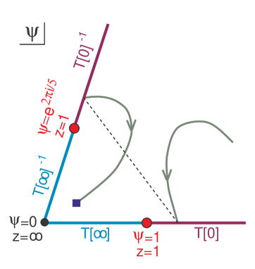
Figure 6: Sketch of the “fundamental wedge” $0<\arg\psi<2\pi/5$ in the $\psi$-plane, a section of Teichmüller space unambiguously parametrized by $z=\psi^{-5}$. Attractor flows have definite charge and are continuous on Teichmüller space, but if we want to represent them exclusively on the fundamental domain, the assigned charge jumps at the wedge boundaries as $q\to q.M$, with $M$ the appropriate monodromy matrix. The labels $T[0]$ and $T[\infty]$ along each branch cut in the picture indicate the monodromy matrix to be applied for $|z|<1$ resp. $|z|>1$. Indicated is an attractor flow line which undergoes a monodromy from a charge $q$ to a charge $q\cdot T[0]$.

This observation can be used to compute numerically the attractor path in moduli space. Suppose we begin with a charge $q$, at an initial modulus $\psi=\psi_{0}$ in the fundamental domain of the $\psi$-plane (see fig. 6). The next point in the path is then approximately given by the point with the smallest $|Z(q)|$ on a small circle around the initial point. By repeating this for a circle around this new point, we find the second point, and so on, producing the approximate path of steepest descent. When a branch cut is approached, at $\arg\psi\in\{0,\frac{2\pi}{5}\}$, we must transform $q$ by an appropriate monodromy as we pass through the cut. If we are traveling down through a cut and $|z|<1$, $T[0]$ should be applied (by right multiplication) to $q$ to determine the new charge, while if $|z|>1$, we should apply $T[\infty]$, as shown in fig. 6. Traveling up through a cut requires us to apply the inverses of these matrices, respectively. The procedure stops when a local minimum of $|Z(q)|$ is reached, that is, at the attractor point.

Notice that it is important to use this step-by-step minimization procedure rather than an arbitrary minimization algorithm, since, as explained in section 3.3, the presence of the conifold point can induce distinct basins of attraction. Therefore particular care should also be taken in the numerical procedure when the flow comes near a conifold point: a too low resolution of the path steps can result in the wrong monodromy matrix being applied to the charge, yielding an incorrect final result for the attractor point.

5.2 Using the integrated BPS equations

The second method is based on equation (11). Suppose we want to compute the flow for a charge $q\equiv(q_{6},q_{4},q_{2},q_{0})$, starting from $z=z_{0}$ (or $\psi=\psi_{0}$). Define for an arbitrary charge $q^{\prime}$ the real function $f(q^{\prime},z)$ as

$$f(q^{\prime},z)=\mathop{\rm Im}\nolimits[Z(q^{\prime})\overline{Z(q)}]\,.$$ (2)

Let $\ell_{1}$ and $\ell_{2}$ be two charges that are mutually local with respect to $q$ (i.e. $\langle\ell_{i},q\rangle=0$), and form together with $q$ a linearly independent set. If $q_{6}$ and $q_{4}$ are not both zero, we can take for instance

$$\ell_{1} = (q_{4},-q_{6},-q_{0},q_{2})$$ (3)

$$\ell_{2} = (0,0,q_{6},q_{4})\,.$$ (4)

If $q_{4}=q_{6}=0$, we can take $\ell_{2}=(q_{1},q_{2},0,0)$ instead. Finally, let $d$ be a (not necessarily integral) charge dual to $q$, i.e. such that $\langle d,q\rangle=1$. For instance, we can take

$$d=(-q_{0},q_{2},-q_{4},q_{6})/(q_{0}^{2}+q_{2}^{2}+q_{4}^{2}+q_{6}^{2})\,.$$ (5)

A convenient parameter for the flow turns out to be

$$\mu\equiv e^{U}\frac{|Z(q)|}{|Z(q)|_{0}}\,,$$ (6)

where $|Z(q)|_{0}\equiv|Z(q)|_{z=z0}=|Z(q)|_{\tau=0}$. This parameter always runs from $1$ to $0$, no matter what nature of the attractor point is (zero central charge or not).

Taking the intersection product of (11) with the $\ell_{i}$ gives, after some reshuffling:

$$f(\ell_{i},z)=f(\ell_{i},z_{0})\,\mu\,.$$ (7)

This is a system of two equations, which can easily be solved (numerically) for $z$ as a function of $\mu$, yielding the desired attractor flow $z(\mu)$ in moduli space. The value of the metric factor $U(\mu)$ along the flow can be computed directly from (6). Finally, to get the $\tau$-dependence, take the intersection product of (11) with the dual charge $d$. This yields:

$$\tau(\mu)=2[f(d,z_{0})-f(d,z(\mu))/\mu]\,.$$ (8)

Thus we obtain the complete solution to the attractor flow equations.

6 Analysis of the quintic

6.1 Some notation and conventions

We will usually work on the $\psi$-plane or the $w$-plane (see below) to describe attractor flows. We take the wedge $0<\arg\psi<2\pi/5$ to be the fundamental domain. Charges will be given in the IIA $(D6,D4,D2,D0)$ $\Pi$-basis of section 4.2. Often however, especially close to the Gepner point $\psi=0$, it is more transparent to give a label based on the $\mathbb{Z}_{5}$ monodromy around the Gepner point. In general, we will use the notation $(q_{6},q_{4},q_{2},q_{0})^{n}$ for the charge $(q_{6},q_{4},q_{2},q_{0}).T[\infty]^{n}$, with $n\in\mathbb{Z}\mathrm{~{}mod~{}}5$. For example $(1,0,0,0)^{1}=(1,1,3,-5)$, which is the state becoming massless at $\psi=e^{2i\pi/5}$. More generally, $(1,0,0,0)^{n}$ becomes massless at $\psi=e^{2ni\pi/5}$. In the type IIB picture, these states correspond to 3-branes wrapped around the appropriate vanishing conifold cycle.

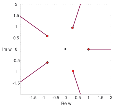
Figure 7: The $w$-plane is a 5-fold cover of moduli space, and is especially convenient for plotting flows. The five fat purple lines are period cuts starting at the conifold point copies $w=e^{2ni\pi/5}$ and running to the large complex structure limit. The black dot in the middle is the Gepner point $\psi=w=0$. Since all periods can be taken to be continuous around $w=0$, we only indicate cuts running to $w=\infty$.

For graphing purposes, we find it convenient to work with a non-holomorphic coordinate $w$ on moduli space, defined as

$$w\equiv\frac{\ln(|\psi|+1)}{\ln 2}\,\frac{\psi}{|\psi|}\,.$$ (1)

This coordinate is proportional to $\psi$ close to the Gepner point, and grows as $\ln|\psi|$ in the large complex structure limit, so we get essentially power-like dependence of the periods on $w$ in both regimes. The normalization of $w$ is chosen such that the copies of the conifold point are located at $w=e^{2ni\pi/5}$, $n=0,\ldots,4$ (see fig. 7).

We will freely mix IIA and IIB language. For instance, we refer to the limit $\psi\to\infty$ both as the large complex structure limit (IIB) and as the large radius limit (IIA).

Our conventional path for interpolating between $\psi=0$ and $\psi=\infty$ is the line $\psi=e^{i\pi/5}\mathbb{R}^{+}$.

We will mostly focus on the analysis of states with low charges, and use supergravity language to describe the corresponding solutions, though the supergravity approximation cannot necessarily be trusted in those cases. However, they can always be trivially converted to large charge solutions by multiplying the charge with a large number $N$, and correspondingly scaling all lengths with a factor $N$. We will come back to this in the discussion section.

6.2 Single flow spectra

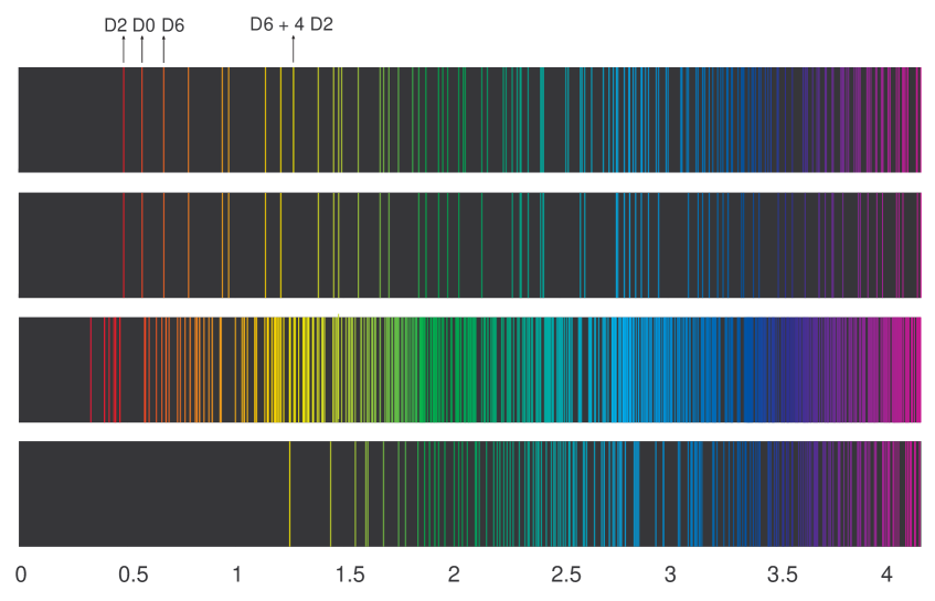
Figure 8: From top to bottom: (1): spectrum of the lightest single flows originating at $\psi=0$. The horizontal axis gives the mass in four dimensional Planck units. The state with pure $D2$ charge (and its $\mathbb{Z}_{5}$ images) has the lowest mass, followed by the $D0$, the $D6$ (which is an empty hole), and five mixed $(D2,D0)$ states. The lightest black hole comes next, with charge $(1,0,4,0)$. (2): Same as (1), excluding the regular black holes. (3): Like (1), but starting at the point $\psi=0.0851-0.3997i$, i.e. the “crash point” of fig. 10. Here the state $(1,0,0,0)^{-1}$ is the lightest. Note that the spectrum lines are more “spread out” here than in (1), due to the fact that the $\mathbb{Z}_{5}$-symmetry is broken, causing the lines to split in five. (4): Masses of regular BPS black holes that exist at the Gepner point, evaluated at their attractor points, where they acquire their minimal value. The lightest charge here is again $(1,0,4,0)$, with $M_{min}\approx 1.250947$.

A first step in analyzing the spectrum from the attractor flow point of view is determining which charges give rise to a well-behaved single flow for a given vacuum modulus, that is, flows not crashing on a regular zero. In other words, these are charges that have a regular BPS black hole solution, or a BPS empty hole solution, or a BPS solution with a mild point-like naked singularity. The latter correspond to $(nD2,mD0)$-charges, which have their attractor point at large radius $\psi=\infty$ [23]. Though the four dimensional supergravity approximation breaks down close to their center (as the quintic decompactifies there), we will consider these solutions to be admissible and in the physical BPS spectrum. Note that the central charges of these $D2-D0$ particles vanish in the large radius limit, so they become massless in four dimensional Planck units. However, since the internal space decompactifies in this limit, the natural scale is the ten dimensional Planck mass, with respect to which the mass of these particles stays finite (for a pure $D0$) or diverges (if $D2$ charge is involved).

A single flow spectrum analysis is illustrated in fig. 8, which resulted from a scan of all charges $(q_{6},q_{4},q_{2},q_{0})^{n}$, with the $q_{i}$ between $-5$ and $5$, and $n$ between $0$ and $4$, together a set of $71,070$ charges (which do not have to be considered all separately, as there are obvious redundancies, such as inversion of all charges and the $\mathbb{Z}_{5}$-symmetry at the Gepner point). Of this set, $31040$ charges can be realized as a single flow.

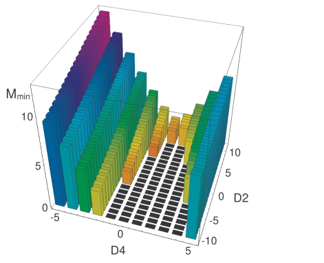
Figure 9: Masses $M_{min}$ evaluated at the attractor points for a set of charges $(1,q_{4},q_{2},0)$, with flows starting at $\psi=0$. A black bar of zero height indicates that the flow does not exist.

As expected from the general arguments in appendix A, our numerical data indicates that the masses of the BPS states indeed tend to grow with charge (see also fig. 9). This is not trivial, since it is not true for the mass of arbitrary candidate BPS charges. At the Gepner point, the BPS mass of a charge $q$ is given by

$$M(q)=c\,\left|(-q_{4}+q_{6})\,\omega^{-1}+(-q_{0}+q_{2}-5q_{4}-2q_{6})+(q_{0}+2q_{4}+q_{6})\,\omega+q_{4}\,\omega^{2}\right|\,,$$

with $c=[5(5+\sqrt{5})/2]^{-1/4}$ and $\omega=e^{2i\pi/5}$. The different terms in this expression correspond to the components of $q$ with respect to the basis $\{(0,0,1,0)^{n}\}$, $n=-1,\ldots,2$. Note that in particular

$$M({q_{6},0,q_{2},0})=c\,|q_{2}-\frac{5-\sqrt{5}}{2}q_{6}|\,,$$ (2)

so no such BPS states should exist at the Gepner point with $q_{2}/q_{6}$ too close to $\frac{5-\sqrt{5}}{2}\approx 1.38197$. This is consistent with our single flow results, as illustrated fig. 9.

6.3 Example of black hole decay from LCS to Gepner point

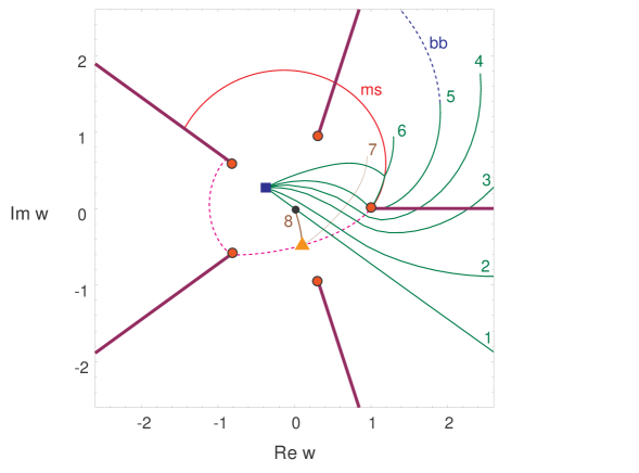
Figure 10: Decay of a BPS state with charge $q=(2,-1,-2,2)$ when moving from large complex structure $w=\infty$ to the Gepner point $w=0$ (see section 6.1 for the relation between $w$ and $\psi$). The state decays into $2(1,0,0,0)+(0,-1,-2,2)=2(1,0,0,0)+(-1,0,-4,0)^{2}$. The green and brown lines $1$ to $8$ are flows with charge $q$, respectively starting at $w_{1}=\infty$, $w_{2}=8\,e^{i\pi/5}$, $w_{3}=4\,e^{i\pi/5}$, $w_{4}=3\,e^{i\pi/5}$, $w_{5}=2.35\,e^{i\pi/5}$, $w_{6}=\,1.6e^{i\pi/5}$, $w_{7}=\,1.2e^{i\pi/5}$, and $w_{8}=0$ (note that the points $w_{1}$, $w_{2}$ and $w_{3}$ are not in the picture). The blue square is a regular attractor point, and the orange triangle a crash-zero. Beyond the basin boundary “bb” separating the good and the bad attractor point, the flow is split. Beyond the marginal stability line “ms”, the state has decayed.

We now turn to the analysis of some split flow examples. As explained in section 3.1, a BPS solution corresponding to a split flow decays when the vacuum moduli are chosen to lie on the line of marginal stability where the split point is located. Such a decay does not necessarily mean that the charge disappears completely from the (supergravity) BPS spectrum: it is perfectly possible that it still exists in a different realization, for example as a single flow.

Most interesting are the cases, though, where the charge does indeed disappear from the BPS spectrum completely when going from one region of moduli space to the other. Such examples highlight qualitative differences in the physics associated to one region or the other.

In fig. 10, we present an example of a charge that exists as a BPS state at large radius, but is (very likely) no longer in the spectrum at the Gepner point. Its charge in the $\Pi$-basis is $\Gamma=q=(2,-1,-2,2)$. At large radius $\psi\to\infty$ it is realized as a single center black hole. In fact, it is a cousin of our lightest BPS black hole state $(1,0,4,0)$, discussed above, since $(2,-1,-2,2)=-(1,0,4,0).T[\infty]^{3}.T[0]^{-1}$. When approaching the Gepner point along the $\arg\psi=\pi/5$ axis, it gets transformed into a split flow with one leg on the conifold point $\psi=1$, by the mechanism of section 3.3: two D6 particles are created at $r=r_{ms}$. When continuing further towards the Gepner point, the line of marginal stability for this split flow is crossed, and the state decays, by expelling the two units of $D6$ charge to spatial infinity.

Our numerical analysis strongly suggests that the charge has disappeared completely from the BPS spectrum at the Gepner point. It is easy to verify that it does not exist there as a single flow. Moreover, it clearly does not exist as a split flow at the “crash point” where $Z=0$. This is quite obvious from energy considerations, or alternatively, it can be argued as follows: there is no room left for the would-be branch running to a split point (since $|Z|$ must decrease along a flow), and there can be no branches running away from it, since if a line of $(\Gamma_{1},\Gamma_{2})$-marginal stability with $\Gamma_{1}+\Gamma_{2}=\Gamma$ ran through the zero, we would have simultaneously $Z(\Gamma_{1})=-Z(\Gamma_{2})$ and $\arg Z(\Gamma_{1})=\arg Z(\Gamma_{2})$, hence $Z(\Gamma_{1})=Z(\Gamma_{2})=0$, and again no flow room is left, which proves the claim. Now, moving away from $Z=0$ upstream the flow, towards the Gepner point, could open up the possibility to have a split flow if $|Z|$ becomes sufficiently large. At the Gepner point, we have $|Z|\approx 1.20751$. Since our numerical data shows beyond reasonable doubt that all regular black holes have mass above $M_{min}\approx 1.250947$ (see fig. 8 (4)), any split flow with charge $\Gamma$ starting from the Gepner point could only have constituent charges with zero attractor mass, i.e. pure $D6$ or $D2-D0$ relatives. However, using the existence criteria for split flows of section 3.1, we excluded (with the help of a computer) the existence of $\Gamma\to\Gamma_{1}+\Gamma_{2}$ split flows with $\Gamma_{1}$ and $\Gamma_{2}$ $\mathbb{Z}_{5}$-relatives of $kD_{6}$ and $nD2+mD0$ charges, with $|k|,|n|,|m|$ smaller than $25$ (greater charge numbers give masses that are way too high along the flow under consideration). A glance at the lower end of the mass spectra in fig. 8, keeping in mind the general arguments of appendix A, shows that this is a quite manageable task. In principle, it is then still possible that more complicated split flows with the given charge exist, with more than two legs of $D6$ or $D2-D0$ type, or with constituents related to $D6$ and $D2-D0$ through more complicated monodromies (with consequently significantly longer, hence more massive, attractor flows). We did not systematically screen those, but based on the study of a large number of candidates (all with negative result), we are convinced that it is extremely unlikely that they would give rise to a valid split flow of the given charge. Finally, as a check on the above reasoning, we (partially) verified the nonexistence of a $(\Gamma_{1},\Gamma_{2})$ split flow starting at the Gepner point for $\Gamma$ as above, by screening a set of $6,765,200$ candidate constituent charges $\Gamma_{1}=\tilde{q}$ with $-25<\tilde{q}_{2j}<25$, using the existence criteria of section 3.1, again with negative outcome.

In conclusion, we predict the existence of a BPS state of charge $(2,-1,-2,2)$ at large radius that does not exist at the Gepner point.

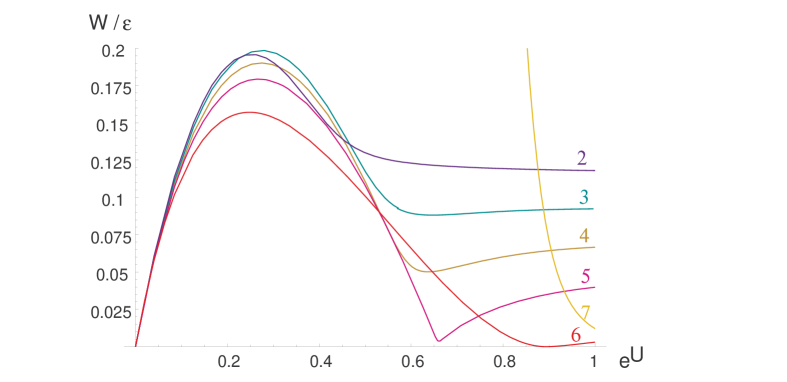
Figure 11: Potentials $W$ for test particle with charge $\epsilon(1,0,0,0)$ in the backgrounds corresponding to the flows in fig. 10. As a convenient radial coordinate, we use the gravitational redshift factor $e^{U}$.

We close this section with a look at the spacetime features of this solution. An instructive way to understand the stability of multicenter BPS configurations corresponding to split flows, is considering the force potential on a test particle of charge $\epsilon\Gamma_{t}$ in the given background [25]:

$$W=2\,\epsilon\,e^{U}\,|Z(\Gamma_{t})|\,\sin^{2}(\frac{\alpha_{t}-\alpha}{2})\,,$$ (3)

where $\alpha_{t}=\arg Z(\Gamma_{t})$. This potential gives the excess energy of the configuration over its BPS energy, is everywhere positive, and becomes zero when $\alpha_{t}=\alpha$, explaining why the constituents of such bound states have to be located at a marginal stability locus in space. Fig. 11 shows this potential $W$ for a test charge $\epsilon(1,0,0,0)$ in the background of a spherically symmetric configurations corresponding to the flows of fig. 10, nicely illustrating the appearance of a BPS minimum upon crossing the basin boundary, and its disappearance upon crossing the line of marginal stability.

6.4 An interesting black hole bound state

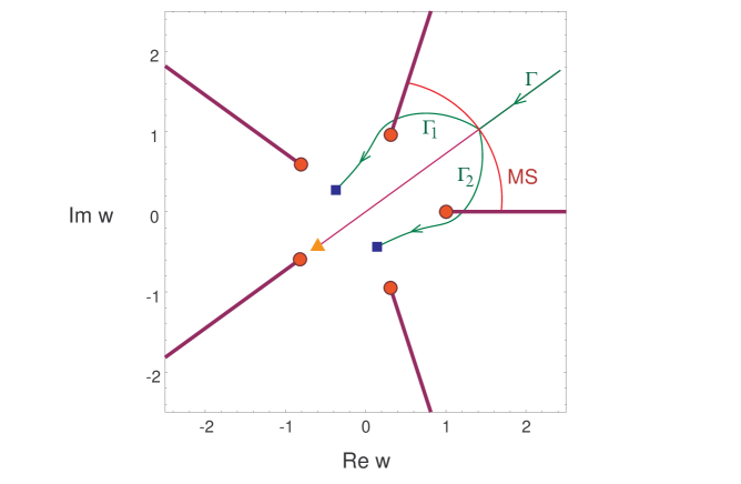
Figure 12: Split flow with regular constituents, which exists at large complex structure, but not at the Gepner point. The total charge is $\Gamma=(0,3,9,-8)$, decaying into $\Gamma_{2}+\Gamma_{1}=(-1,1,4,-1)+(1,2,5,-7)=(1,0,4,0).T[0]^{-1}+(1,0,4,0).T[0].T[\infty]$. The purple line extending the incoming branch at the split point is the would-be single flow, crashing on a regular zero at the orange triangle.

It is fairly easy to find split flows with two regular black hole constituents that also have a regular single flow representation. Finding examples without the latter turns out to be much more difficult. One example, with charge $q=(0,3,9,-8)$, is given in fig. 12.

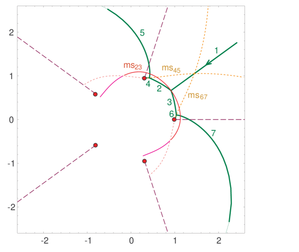
Figure 13: Alternative split flow to fig. 12: the initial branch (1) of charge $(0,3,9,-8)$ splits at the MS line $\mathrm{ms}_{23}$ in a branch (2) of charge $(3,3,10,-11)=(0,0,1,3)^{1}$ and a branch (3) of charge $(-3,0,-1,3)=(0,0,-1,2)^{-1}$. Branch (2) then splits on $\mathrm{ms}_{45}$ as (4): $3(1,0,0,0)^{1}$ $+$ (5): $(0,0,1,4)$ and similarly (3) on $\mathrm{ms}_{67}$ as (6): $3(-1,0,0,0)$ $+$ (7): $(0,0,-1,3)$. Note that the split flows (245) and (367) can be created from single flows (of $D0-D2$ type) by the conifold branch creation mechanism of section 3.3.

However, this example has an alternative split flow realization, with decay line closer to the Gepner point than the one displayed in fig. 12. This is shown in fig. 13. The flow has four legs, with none of them corresponding to a regular black hole constituent: two are of empty hole type (D6-like), and two of mildly naked type (D0-D2-like).

Again, we did a screening of possible constituents for this charge, at $w=2\,e^{i\pi/5}$, checking $6,765,200$ candidate charges $\tilde{q}$, with the $\tilde{q}_{2j}$ ranging from $-25$ to $25$. The only two possibilities that came out are those given in fig. 12 and 13. Therefore, in particular, we expect this charge to be absent from the BPS spectrum at the Gepner point, with a somewhat lower level of confidence though (it becomes slightly less unlikely that more complicated split flows exist).

Incidentally, we did not find any example of a charge that can only be realized as a split flow with exclusively regular black holes as constituents (i.e. like fig. 12 but then without the alternative of fig. 13), but our search for those was not sufficiently systematic to be conclusive.

6.5 Multiple basins of attraction

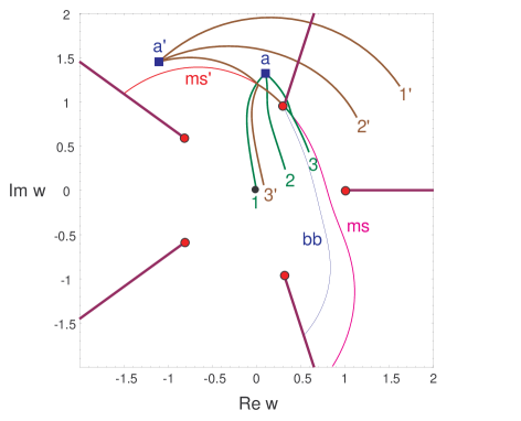
Figure 14: The charge $q=(0,-3,10,18)=(1,-3,-5,-1)^{1}$ has two different basins of attraction in the fundamental domain $0<\arg\psi<2\pi/5$, separated by the blue basin boundary labeled “bb”. Attractor point $a$ has $|Z_{*}|=6.045$, while attractor point $a^{\prime}$ has $|Z_{*}|=5.603$, so the corresponding near horizon geometries and entropies of the black holes are not equal. The green (brown) lines $1,2,3$ ($1^{\prime},2^{\prime},3^{\prime}$) are a continuous family of flows attracted to $a$ ($a^{\prime}$), with $3$ and $3^{\prime}$ the split flows obtained upon crossing the basin boundary. Those split flows decay at the marginal stability lines $ms$ resp. $ms^{\prime}$.

In the previous sections, we have already seen some examples of multiple basins of attraction induced by the presence of conifold points. Those were all cases where one of the basins did not have a good attractor point but a zero instead. The example presented in fig. 14 shows that it is also possible to have different basins with each a regular attractor point, yielding different black holes, with different entropies. Recall however that there is no continuous way to deform the one black hole into the other (while keeping the BPS property), so there is no physical consistency problem.

On the full Teichmüller space, there will in general be infinitely many different basins of attraction, corresponding to the infinitely many ways one can run around the conifold point copies. This multitude of basins is in strong contrast with the five dimensional case, where different basins occur much less generically [43].

6.6 The D6-D2 system and comparison with the LCSL approximation

In the large complex structure limit (LCSL), it is possible to solve explicitly equation (13) determining the attractor point [45, 23]. The starting point are the asymptotic expressions (12)-(15) for the periods, dropping the constant term for $\Pi_{D6}$. Consider a charge $q=(q_{6},q_{4},q_{2},q_{0})$. It is useful to define the following shifted (nonintegral) charges:

$$\hat{q}_{2} = q_{2}-{\textstyle\frac{11}{2}}\,q_{4}-{\textstyle\frac{25}{12}}\,q_{6}$$ (4)

$$\hat{q}_{0} = q_{0}+{\textstyle\frac{25}{12}}\,q_{4}\,.$$ (5)

¿From the results of [45, 23], it follows that the mass $M_{*}$ at the attractor point is given by

$$M_{*}^{4}={\textstyle\frac{1}{3}}\,{\hat{q_{2}}}^{2}\,{q_{4}}^{2}+{\textstyle\frac{8}{45}}\,{\hat{q_{2}}}^{3}\,q_{6}+2\,\hat{q_{0}}\,\hat{q_{2}}\,q_{4}\,q_{6}+{\textstyle\frac{10}{3}}\,\hat{q_{0}}\,{q_{4}}^{3}-{\hat{q_{0}}}^{2}\,{q_{6}}^{2}\,,$$ (6)

provided this quantity is positive. The attractor point $t_{*}$ itself is given by:

$$t_{*}=\frac{(q_{4}\,\hat{q_{2}}-3\,q_{6}\,\hat{q_{0}})\,+\,3\,{M_{*}}^{2}\,i}{5\,{q_{4}}^{2}+2\,q_{6}\,\hat{q}_{2}}\,.$$ (7)

If (6) is negative, the flow crashes at a regular zero and (13) does not have a solution $t_{*}$. Also, the large complex structure approximation can only be trusted if $t_{*}\gg 1$ (though we observed pretty good agreement with the full numerical results for $t_{*}>1$).

Note that there are no multiple basins of attraction in this approximation: $t_{*}$ is unambiguously fixed by the charge. This is not surprising, since the LCSL approximation is blind for the presence of the conifold point. Furthermore, as it should, the expression for $M_{*}$ is invariant under the monodromy $q\to q\cdot T[0]$, while the expression for $t_{*}$ transforms as $t_{*}\to t_{*}+1$.

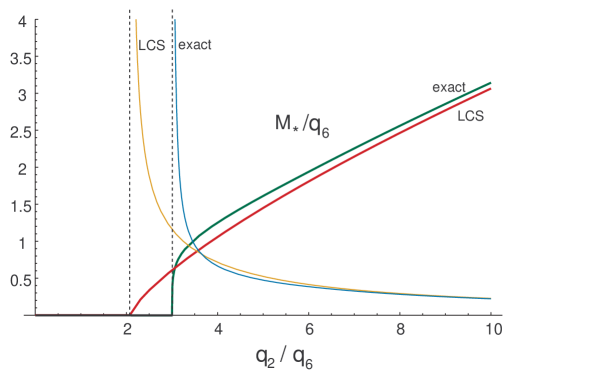
Figure 15: Comparison of numerical results with the LCSL approximation for charge $(q_{6},0,q_{2},0)$, $q_{6}>0$, where $q_{2}/q_{6}$ is varied continuously over the $x$-axis. The lines hitting zero give the relative attractor mass $M_{*}/q_{6}$ for the given charge, with the zero corresponding to the critical point for existence of a single flow. The lines diverging at those zeros indicate the mass of the “dual” charge defined in (5), with the divergence corresponding to reaching a boundary of Teichmüller space. Note that the exact $M_{*}$ curve is much steeper near its critical point than the LCS curve near its critical point. This implies that the near-critical single flow mass spectrum will be much more dilute in the exact than in the LCS case.

An interesting special case is a pure $D6-D2$ system, i.e. $q_{4}=0$, $q_{0}=0$. Then the above equations simplify to

$$\hat{q}_{2} = q_{2}-{\textstyle\frac{25}{12}}\,q_{6}$$ (8)

$$\hat{q}_{0} = 0$$ (9)

$$M_{*}^{4} = {\textstyle\frac{8}{45}}\,{q_{6}}^{4}\,(q_{2}/q_{6}-{\textstyle\frac{25}{12}})^{3}$$ (10)

$$t_{*} = i\,\sqrt{{\textstyle\frac{2}{5}}(q_{2}/q_{6}-{\textstyle\frac{25}{12}})}\,.$$ (11)

Therefore, according to the LCSL approximation, we need $q_{2}/q_{6}\geq\frac{25}{12}\approx 2.08333$ for the flow to exist. At the critical value, we have $t_{*}=0$. This is a boundary point of the LCSL Teichmüller space, which is a general feature of critical charges, as can be seen directly from (13) or (2).

Our numerical results on the other hand indicate that the exact condition for the existence of a flow is $q_{2}/q_{6}\geq 3$. At this critical value, we have $q\sim(0,0,2,1)^{2}$, and the attractor point is indeed again a boundary point, $\psi=-\infty$. A more detailed comparison of the exact and LCSL cases is shown in fig. 15.

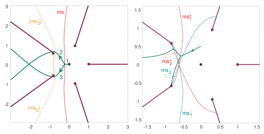
Figure 16: Two possible split flows with charge $q=(3,0,8,0)$, near the Gepner point. Left: two-legged realization, with one leg (2) of charge $(-2,-2,-7,7)=-(0,0,1,2)^{1}$ and the other one (3) of charge $(5,2,15,-7)=(0,0,-1,1)^{3}$. Note that when the starting point is moved up sufficiently, branch (3) gets an additional conifold leg, with marginal stability line $ms_{3}$. Right: For starting points above the real $w$-axis, we get an alternative split flow of the form $(3,0,8,0)\to(1,0,0,0)^{3}+[(0,0,-2,-3)^{-1}\to(1,0,0,0)^{2}+(0,0,-2,-1)^{2}]$, with MS lines $ms_{1}^{+}$ resp. $ms_{2}^{+}$. For starting points below the real axis, one gets a similar but reflected configuration. For points on the real axis, there is only one split point, with three outgoing branches.

It is plausible that the critical point for the single flow BPS spectrum is also the critical point for the general flow BPS spectrum in the LCSL approximation (we did not study this question systematically though). However, in the exact case, this is certainly not true. In fact, there is a rich set of split flows with charge quotient below the single flow critical value $q_{2}/q_{6}=3$. We do not know how far below this value one can go with split flows, but from the discussion at the end of section 6.2, it follows that this is certainly only a finite amount.

One example is the “mysterious” BPS state $|10000\rangle_{B}$ discovered in [2] and given a split flow interpretation in [25]. The charge of this state is $(2,0,5,0)$, so indeed $q_{2}/q_{6}=2.5<3$. It exists at the Gepner point, but decays when moving along the negative $\psi$-axis. The decay products are $(1,0,0,0)^{2}$ and $(1,0,0,0)^{3}$. These are the only possible decay products that came out of the screening of our usual $6,765,200$ candidate constituents with $-25<\tilde{q}_{2j}<25$. Another example is given in fig. 16. Here we have $q_{2}/q_{6}=8/3\approx 2.666667$. At the Gepner point, there are two possible realizations, again the only ones resulting from the screening procedure.

Many other examples can be constructed. It would be interesting to study the spectrum of such “sub-critical” split flows systematically.

6.7 The monodromy stability problem

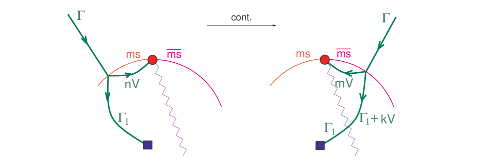
Figure 17: The split flows on the left and the right are related by continuous variation of the starting point. By charge conservation, we have $\Gamma=\Gamma_{1}+nV=\Gamma_{1}+(m+k)V$, and by the Picard-Lefshetz theorem $k=\langle\Gamma_{1},V\rangle$. The purple wiggly line is the cut corresponding to the conifold monodromy. The red line $ms$ is the $(\Gamma_{1},nV)$-marginal stability line; the pink line $\overline{ms}$ is the “conjugate” $(\Gamma_{1},-nV)$-marginal stability line (as $Z(V)$ flips sign upon crossing the conifold singularity).

Common ${\mathcal{N}}=2$ lore states that BPS states can only decay when a line of marginal stability is crossed, or, in the split flow picture, when the incoming branch shrinks to zero size. However, a paradox arises in some cases, due to monodromy effects. Consider, as in fig. 17, a split flow with one leg on a conifold point, carrying a charge $nV$, where $V$ is the charge with vanishing mass at the conifold point. The other leg carries an arbitrary charge $\Gamma_{1}$. When the starting point of the flow is continuously moved to the right and all goes well, the configuration should transform to one with a leg of charge $mV$, as indicated in the picture, by the mechanism of section 3.3. The integers $n$ and $m$ are related by

$$n=m+\langle\Gamma_{1},V\rangle\,.$$ (12)

Consistency requires that the $(\Gamma_{1},-nV)$-MS line (labeled $\overline{ms}$ in the figure) is also a $(\Gamma_{1}+kV,mV)$-MS line. This is the case if and only if

$$mn\leq 0\,.$$ (13)

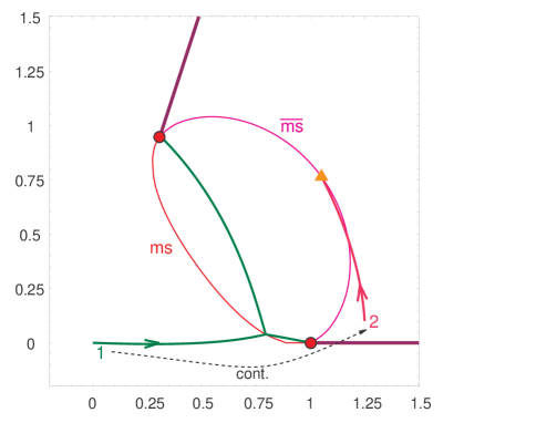
Figure 18: When the starting point of the split flow $(7,1,3,-5)\to 6(1,0,0,0)+(1,0,0,0)^{1}$ is continuously transported as indicated, it ceases to exist: it crashes on the would-be line of marginal stability. The transport is counterclockwise with respect to the conifold point (whereas in fig. 17, it was clockwise), so we have here $m=6$, $n=6+\langle(1,0,0,0)^{1},(1,0,0,0)\rangle=6-5=1$, and $nm=6$, which does not satisfy (13).

To show that this situation can indeed occur in practice for the quintic, and to illustrate what happens if the above condition is not satisfied, we give a specific example not satisfying the consistency condition in fig. 18. The figure shows that when the starting point crosses the basin boundary induced by the conifold point (i.e. the critical incoming flow passing through that point), we get a flow crashing on the $\overline{ms}$-line. So the BPS solution ceases to exist. In general, there might of course still exist other BPS realizations of the given charge, but we cannot reach these continuously in this way.

So we are facing a paradox again. One could contemplate the possibility that the BPS state just decays into other BPS particles at the basin boundary, but this is not a satisfying solution: apart from the fact that there is no smooth spacetime description of such a hypothetical decay, it follows directly from equation (11) that a basin boundary, being an attractor flow, can never be a marginal stability line of mutually nonlocal charges, and is very unlikely to be a marginal stability line for suitable mutually local charges.

A more attractive way out, at least at the supergravity level, is that the BPS state transforms into a non-BPS state. This is suggested by studying the test particle potential for charge $\epsilon V$: indeed, upon crossing the basin boundary, the minimum of the potential gets lifted to a nonzero value, like in fig. 11. However, at the quantum level, such a transition is usually considered unlikely, because a non-BPS supermultiplet has more states than a BPS multiplet, so to match the number of states, BPS states should pair up, which would require a non-generic degeneracy of distinct BPS multiplets. It is not impossible that this is precisely what happens here, but we do not know how exactly it would work.

Another possibility is that the configuration was not BPS to begin with, either because of quantum subtleties, or because of subtleties arising already at the classical level in the construction of truly solitonic multicenter supergravity solutions involving empty hole charge, discussed briefly (but inconclusively) at the end of section 2.2.2. Support for this possibility is given by the strong analogy with the multi-pronged string picture of BPS states in quantum field theory [37], where similar spurious multi-pronged strings arise, which are discarded on the basis monodromy arguments, or by lifting the strings to M-theory 2-branes. This is the so-called “s-rule”. In [38], where BPS solutions of ${\mathcal{N}}=2$ effective Yang-Mills theories were studied, a very similar problem as the one discussed in this section was encountered: the s-rule did not seem to emerge — or at least not in an obvious way — from the analysis of possible solutions.

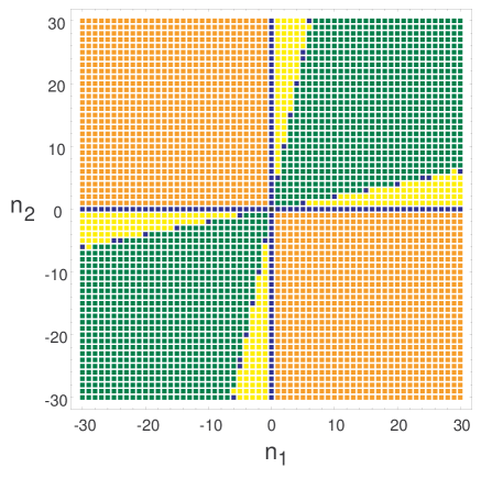
Figure 19: Split flow spectrum at the Gepner side of the MS ellipsoid for flows with a charge $n_{1}$ leg on $(1,0,0,0)$ and a charge $n_{2}$ leg on $(1,0,0,0)^{1}$. The orange dots ($n_{1}n_{2}<0$) indicate charges that do not have a split flow realization, the yellow dots are the charges that have a split flow realization, but one that is unstable under repeated monodromy around the MS ellipsoid, and the green and blue dots are the monodromy stable split flows, with the blue dots the charges related to pure $(1,0,0,0)$ or the pure $(1,0,0,0)^{1}$ charge.

Whatever may be the correct answer, an interesting question associated for example to the case shown in fig. 18, is which split flows stay within the spectrum no matter how many times one encircles the marginal stability ellipsoid generated by the two conifold point copies considered there. This gives an infinite set of consistency conditions, arising from both conifold points. If we write the charge $q$ as

$$q=n_{1}\,(1,0,0,0)+n_{2}\,(1,0,0,0)^{1}\,,$$ (14)

and denote the intersection product of the “right” charge with the “left” charge by $\kappa$ (so here, $\kappa=5$ at the Gepner side of the MS-ellipsoid, and $\kappa=-5$ at the LCS side), then we found, after a somewhat lengthy analysis that we will not give here, the following criterion to be in the “monodromy stable” part of the spectrum: either the charge has to be related by a (multiple) monodromy around the MS ellipsoid to pure $(1,0,0,0)$ or pure $(1,0,0,0)^{1}$ charge, or it has to satisfy

$$\frac{1}{\lambda}n_{2}\leq n_{1}\leq\lambda\,n_{2}\,,$$ (15)

with

$$\lambda=\frac{1}{2}(\kappa+\sqrt{\kappa^{2}-4})\,.$$ (16)

As a check, note that in the well-known $SU(2)$ Seiberg-Witten case, where $\kappa=\pm 2$, this condition indeed reproduces the BPS spectrum. In the quintic case at hand, we find at the Gepner side $\lambda_{G}=\frac{1}{2}(5+\sqrt{21})\approx 4.79129$, and at the LCS side $\lambda_{L}=-1/\lambda_{G}$. The resulting monodromy stable spectrum at the Gepner side is shown in fig. 19.

It is not inconceivable that the subtleties we see appearing here are related to the $\mathbb{R}$-valued gradings of the subobjects of [7, 14]. It would be interesting to analyze the states of this section in that framework.

6.8 The surface area of empty holes and composites is bounded from below.

An intriguing feature of all BPS solutions described here is that they generically have a minimal size, in the sense that the surface enclosing the region in which the sources can be localized has, for a given total charge $\Gamma=q$ but arbitrary moduli values, always a nonzero minimal area. In view of the holographic principle, this is perhaps not surprising, but at the level of the equations and their solutions, this is not obvious at all, since for instance the coordinate radius can be made arbitrarily small.

The smallest area we have found is that of the black hole with charge $(1,0,4,0)$ (and its cousins under the duality group): $A_{\mathrm{min}}=19.664719$.

For regular black holes, the above minimal area statement is of course obvious. For composites, say a charge $\Gamma_{1}$ surrounded by a homogeneous shell of total charge $\Gamma_{2}\equiv(\tilde{q}_{6},\tilde{q}_{4},\tilde{q}_{2},\tilde{q}_{0})$, we will prove this now. Note that in general, one can expect the object to become minimal in size in the large complex structure limit, because the flow will become infinitely long then, and longer flows correspond usually to smaller cores. Therefore, we should in particular consider this limit and show that the asymptotic area is finite.

We can assume $(q_{6},q_{4})\neq 0$ because composites of $D2-D0$ type do not exist in the large radius limit. Define $\ell_{1}$ and $\ell_{2}$ as in (3)-(4). Taking the intersection product of the $\ell_{i}$ with (11) gives:

$$e^{-U}\,\mathop{\rm Im}\nolimits[e^{-i\alpha}Z(\ell_{i})]=\mathop{\rm Im}\nolimits[e^{-i\alpha}Z(\ell_{i})]_{\infty}\,.$$ (17)

Denoting the point where the flow splits by $z_{*}$, this implies that the value of $U$ there, $U_{*}$, is given by:

$$e^{-U_{*}}=\frac{\mathop{\rm Im}\nolimits[\bar{Z}Z(\ell_{1})]_{\infty}}{\mathop{\rm Im}\nolimits[\bar{Z}Z(\ell_{1})]_{*}}\,.$$ (18)

Combining this with equation (19) for $r_{*}=r_{ms}$ and the form of the metric (6) yields

$$A_{*}=4\pi e^{-2U_{*}}r_{ms}^{2}=\pi\langle\Gamma_{1},\Gamma_{2}\rangle^{2}\,\frac{1}{\left(\mathop{\rm Im}\nolimits[e^{-i\alpha}Z(\ell_{1})]_{*}\right)^{2}}\,\left(\frac{\mathop{\rm Im}\nolimits(\bar{Z}Z(\ell_{1}))_{\infty}}{\mathop{\rm Im}\nolimits(\bar{Z}Z(\Gamma_{2}))_{\infty}}\right)^{2}\,.$$ (19)

As expected, the only vacuum values of the moduli where our minimal area statement could go wrong is where some central charges diverge, that is, in the large complex structure limit $\psi\to\infty$. However, note that in this limit $\mathop{\rm Im}\nolimits[e^{-i\alpha}Z(\ell_{2})]_{\infty}=0$, because the central charges of the $D2$ and the $D0$ are zero at large complex structure (due to the Kähler potential factor). Therefore, equation (17) tells that for all $z$ along the flow, we have $\mathop{\rm Im}\nolimits[e^{-i\alpha}Z(\ell_{2})]_{\infty}=0$; that is, in the limit under consideration, our flow is just a $(\ell_{1},\Gamma)$ (anti-)marginal stability line, and the point $z_{*}$ is the intersection of this line with the $(\Gamma_{1},\Gamma_{2})$ marginal stability line. So the second factor in $(\ref{Aformula})$ will converge to a fixed finite value. As for the third factor, using the asymptotic expressions for the periods given in appendix B, a direct computation gives

$$\lim_{\psi\to\infty}\,\frac{\mathop{\rm Im}\nolimits(\bar{Z}Z(\ell_{1}))_{\infty}}{\mathop{\rm Im}\nolimits(\bar{Z}Z(\Gamma_{2}))_{\infty}}=\frac{q_{4}^{2}+q_{6}^{2}}{q_{6}\tilde{q}_{4}-q_{4}\tilde{q}_{6}}\,.$$ (20)

In conclusion, we find for the area of the core, in the large complex structure limit:

$$A_{*}=\frac{\pi\langle\Gamma_{1},\Gamma_{2}\rangle^{2}}{\left(\mathop{\rm Im}\nolimits[e^{-i\alpha}Z(\ell_{1})]_{*}\right)^{2}}\,\left(\frac{q_{4}^{2}+q_{6}^{2}}{q_{6}\tilde{q}_{4}-q_{4}\tilde{q}_{6}}\right)^{2}\,.$$ (21)

As an example, one finds for the minimal surface area of the state $|10000\rangle_{B}$ (with $q=(2,0,5,0)$) discussed in [2, 25]: $A_{*}=43.0607$.

For the empty hole, we can make a similar reasoning. Let us consider the case of N units of pure D6-brane charge. Taking the intersection product of (11) with pure D2-brane charge resp. pure D0-brane charge, we get

$$e^{-U}\mathop{\rm Im}\nolimits(e^{-i\alpha}Z_{2}) = \mathop{\rm Im}\nolimits(e^{-i\alpha}Z_{2})_{\infty}$$ (22)

$$2e^{-U}\mathop{\rm Im}\nolimits(e^{-i\alpha}Z_{0}) = N\tau+2\mathop{\rm Im}\nolimits(e^{-i\alpha}Z_{0})_{\infty}\,.$$ (23)

Taking the moduli at spatial infinity to the large complex structure limit $\psi=\infty$, this becomes

$$\mathop{\rm Im}\nolimits(e^{-i\alpha}Z_{2}) = 0$$ (24)

$$2e^{-U}\mathop{\rm Im}\nolimits(e^{-i\alpha}Z_{0}) = N\tau\,.$$ (25)

The first equation implies that the flow coincides with the real $\psi$-axis, with $\psi>1$, where $Z_{6}$ and $Z_{2}$ are positive imaginary. So the second equation yields for the area of the core of the empty hole, where the attractor point $\psi=1$ is reached:

$$A_{*}=4\pi(e^{U_{*}}\tau_{*})^{-2}=\frac{\pi N^{2}}{(\mathop{\rm Re}\nolimits Z_{0})^{2}_{\psi=1}}\approx 43.91946\,N^{2}\,.$$ (26)

Again, the finiteness of the area is not trivial, since $\tau_{*}\to\infty$ and $e^{U_{*}}\to 0$ in this limit (as can be seen by intersecting (11) with $D4$-charge).

6.9 Near horizon flow fragmentation

Consider a regular BPS black hole of charge $\Gamma$. In the near-horizon limit, or equivalently in asymptotically $\mathrm{AdS}_{2}\times S^{2}$ space, many of the features discussed above change quite drastically. The split flow picture still holds, but now with the starting point at the $\Gamma$-attractor point. The constant term in 17 drops out, and as a result the constraint on the source positions becomes, instead of (18),

$$\sum_{q=1}^{N}\frac{\langle\Gamma_{p},\Gamma_{q}\rangle}{|{\bf x}_{p}-{\bf x}_{q}|}=0\,.$$ (27)

Consequently, multicenter configurations are also generically allowed for mutually local charges. All this implies we get in general a plethora of possible realizations of the system as a multicenter BPS solution, generalizing the AdS-fragmentation phenomenon described in [46]. Note however that from the point of view of an observer far away from the black hole, all these different solutions will be indistinguishable. If a counting of the statistical entropy within this low energy framework were possible, the number of different ways of “fragmenting” the flow in constituents would presumably give a significant contribution to the entropy.

7 Conclusions

We discussed a variety of (at least suggestive) results on the stringy BPS spectrum of type II Calabi-Yau compactifications that can be obtained in the framework of BPS supergravity solutions and their associated split flows, and illustrated this in detail for the example of type IIA theory on the quintic. Among the specific predictions we obtained for this example (with various degrees of confidence) are the following:

• There are infinitely many BPS states at any point in moduli space. In particular, the set of rational boundary states at the Gepner point constructed in [2] is only a small fraction of the total spectrum.

• The lightest possible regular BPS black hole with charge $Nq$ (in the $\Pi$-basis of section 4.2) has mass equal to $NM_{min}$, with $M_{min}\approx 1.250947$, $q=(1,0,4,0)$, and lives in a vacuum with the value at spatial infinity of $\psi\approx 0.375603$. From equation (10), it follows that about $15.44\%$ of its mass there is due to worldsheet instanton corrections.

• The mass spectrum of BPS states is generically discrete and without accumulation points.

• A BPS state with charge $q=(2,-1,-2,2)$ exists at large radius, but not at the Gepner point. Its decay products are two pure $D6$ branes and a cousin of our “lightest black hole” particle with charge $q=(0,-1,-2,2)=-(1,0,4,0)^{2}$ (see section 6.1 for the superscript notation).

• BPS states have usually several distinct low energy realizations (e.g. as a single center black hole, and as one or more multicenter configurations with mutually nonlocal components). Each possible composite has its own marginal stability line and decay products. The decay products of a state are therefore in general not fixed by its charge alone.

• The charge $q=(0,3,9,-8)$ has at large radius a realization as a composite of two regular black holes, of charge $(-1,1,4,-1)=(1,0,4,0)\cdot T[0]^{-1}$ and $(1,2,5,-7)=(1,0,4,0)\cdot T[0]\cdot T[\infty]$, but not as a single center black hole. It has an alternative realization with four non-black hole constituents related to $D6$ and $D2-D0$ type charges as shown in fig. 13. At $w=2e^{i\pi/5}$ (and downstream the attractor flow from there), these are probably the only two possible realizations. The second one decays closer to the Gepner point than the first one.

• Multiple basins of attraction, with different corresponding black hole entropies, are a generic — and perfectly consistent — feature in the presence of conifold points.

• Below the critical value $q_{2}/q_{6}=3$ (but not too much) where $D6-D2$ charges can no longer be represented as black holes, there is a rich set of composite realizations of these charges. They all involve constituents related to charges of $D6$ and $D2-D0$ type.

• “Monodromy-stable” bound states of the D6 $(q=(1,0,0,0))$ and its cousin $q=(1,0,0,0)^{1}$, at the Gepner point, are given by fig. 19. An example is (a $\mathbb{Z}_{5}$-relative of) the state $|10000\rangle$ of [2], with charge $q=(2,1,3,-5)=(2,0,5,0)^{3}=(1,0,0,0)+(1,0,0,0)^{1}$.

• No matter how one tunes the moduli, one can never localize $N$ sources in an area less than about $20N^{2}$ in Planck units, whether the object is a black hole or not (at least for BPS solutions).

• On the horizon of a BPS black hole, there is a large enhancement of possibilities of multicenter configurations.

It is actually quite surprising that the split flow picture, if taken seriously, has so much predictive power on the BPS spectrum: a priori, it would seem that an enormous amount of possible split flows would be allowed, much more than the possible decays allowed by the microscopic picture, but — at least for charges with low mass — this turns out not to be the case; for instance the fact that out of the $6,765,200$ candidate constituents we screened for the above discussed charges, only one or two were actually valid, is quite remarkable.

Notice however that we have made quite a big leap in faith in accepting this really as a trustworthy prediction. Indeed, we have made our arguments for low charge numbers, for which supergravity cannot necessarily be trusted, and while any low charge solution can always be promoted to a high charge solution by simply scaling everything up with a large factor $N$, the opposite is not true. In particular, this means that in screening the possible constituents of the charges under consideration, we were certainly not screening all possible constituents of its large $N$ counterpart. So strictly speaking, the arguments for nonexistence of other split flows for e.g. $q=(2,-1,-2,2)$ apart from the ones we presented, have little physical foundation in low energy supergravity itself. However, since a large part of the argument relies purely on energy conservation considerations (e.g. the fact that the state at the Gepner point is too light to decay in BPS states corresponding to regular flows), it is not entirely unfounded. And more importantly, it cannot be denied that the split flow picture actually works. A natural conjecture would therefore be that this picture should also arise somehow from microscopic considerations, like it does in the description of QFT BPS states as (possible multi-pronged) strings [36, 37]. Clearly it would be very interesting if this were indeed the case. The idea is not that wild though, since the basic structures underlying BPS objects quite universally tend to be valid in a wide range of regimes, though their interpretation can vary considerably.

Another loose end is the monodromy stability (or “s-rule”) problem discussed in section 6.7. Some input from the microscopic picture, or perhaps a deeper analysis of full multicenter solutions involving $D6$-like charges, could resolve this puzzle.

In conclusion, we believe we have convincingly demonstrated that, while it is probably not the ideal device to get insight in the underlying organizing structures, the split flow picture can nevertheless provide valuable information, and some quite concrete intuition, on the problem of BPS spectra of type II Calabi-Yau compactifications at arbitrary moduli values.

Appendix A (Split) flows as geodesic strings and discreteness of the spectrum

An interesting link, useful to give some intuition for the spectrum, can be made between (split) attractor flows and the “7/3/1”-brane picture of BPS states in rigid ${\mathcal{N}}=2$ quantum field theories [36, 37]. This comes from the observation [25] that attractor flows can be considered to be geodesic “strings” in moduli space. Split flows can similarly be interpreted as geodesic multi-pronged strings. This follows from the fact that attractor flows in moduli space are minima of the action

$$S=|Z_{*}|+\int\sqrt{V}ds\,,$$ (1)

where the startpoint of the string is kept fixed at the vacuum moduli, $Z_{*}$ is $Z(\Gamma)$ evaluated at the free endpoint(s) of the string, $V=4g^{a\bar{b}}\partial_{a}|Z|{\bar{\partial}}_{\bar{b}}|Z|$, and $ds$ is the line element on moduli space: $ds^{2}=g_{a\bar{b}}dz^{a}d\bar{z}^{\bar{b}}$. Requiring $\delta S=0$ for variations of the free endpoint fixes the latter to be located at the attractor point of $\Gamma$. The mass $|Z(\Gamma)|_{\mathrm{vac}}$ of the BPS supergravity solution equals the minimal value of the action $S$.

This picture makes it plausible that in any finite region $F$ of moduli space (or, more precisely, its covering Teichmüller space), away from singularities, the mass spectrum of (split) flows (and therefore of BPS supergravity solutions) is discrete without accumulation points and at most finitely degenerate. To see this, first note that at a regular $\Gamma$-attractor point, equation (13) implies

$$|Z(\Gamma)|_{*}\geq\frac{1}{2}\frac{|\langle\Gamma^{\prime},\Gamma\rangle|}{|Z(\Gamma^{\prime})|}\,,$$ (2)

for any $\Gamma^{\prime}$. If the attractor point is in or not too far away from our finite singularity-free region $F$, $|Z(\Gamma^{\prime})|$ can be bounded from above, and therefore the first term in (1) will be bounded from below. Furthermore, since the right hand side of (2) is proportional to the charge $\Gamma$, this bound should grow roughly proportional to the “magnitude” of the charge $\Gamma$. On the other hand, if the attractor point is far away from the region $F$ (such that $|Z(\Gamma^{\prime})|$ can no longer be bounded), the attractor flow going to that point will be long, and consequently the second term in (1) will be large, or at least bounded from below. Again, this term will scale roughly proportional to $\Gamma$.

This makes it plausible that the spectrum will indeed be discrete and without accumulation points, something that is also strongly supported by the numerical data we obtained for the quintic. Of course, a rigorous proof would require a much more lengthy analysis, but we will not try this here.

Appendix B Precise expressions for the quintic periods

In this appendix, to facilitate reproduction and extension of our numerical explorations by the interested reader, we will give the detailed expressions for the quintic periods in terms of the pre-defined Meijer functions of the Mathematica software package. This is not entirely trivial, since the presence of monodromies make these definitions convention-dependent. We will use Mathematica syntax to denote the Meijer functions.

Define

$$c=\frac{1}{\Gamma(\frac{1}{5})\Gamma(\frac{2}{5})\Gamma(\frac{3}{5})\Gamma(\frac{4}{5})}\,\,\,\,\,,$$ (3)

$$U_{0}^{-}(z) = c\,\mathrm{MeijerG}[\{\{{\textstyle\frac{4}{5}},{\textstyle\frac{3}{5}},{\textstyle\frac{2}{5}},{\textstyle\frac{1}{5}}\},\{\}\},\{\{0\},\{0,0,0\}\},-z]$$ (4)

$$U_{1}^{-}(z) = {\textstyle\frac{c}{2\pi i}}\mathrm{MeijerG}[\{\{{\textstyle\frac{4}{5}},{\textstyle\frac{3}{5}},{\textstyle\frac{2}{5}},{\textstyle\frac{1}{5}}\},\{\}\},\{\{0,0\},\{0,0\}\},z]$$ (5)

$$U_{2}^{-}(z) = {\textstyle\frac{c}{(2\pi i)^{2}}}\mathrm{MeijerG}[\{\{{\textstyle\frac{4}{5}},{\textstyle\frac{3}{5}},{\textstyle\frac{2}{5}},{\textstyle\frac{1}{5}}\},\{\}\},\{\{0,0,0\},\{0\}\},-z]$$ (6)

$$U_{3}^{-}(z) = {\textstyle\frac{c}{(2\pi i)^{3}}}\mathrm{MeijerG}[\{\{{\textstyle\frac{4}{5}},{\textstyle\frac{3}{5}},{\textstyle\frac{2}{5}},{\textstyle\frac{1}{5}}\},\{\}\},\{\{0,0,0,0\},\{\}\},z]\,,$$ (7)

and

$$U_{0}^{+}(z) = U_{0}^{-}(z)$$ (8)

$$U_{1}^{+}(z) = U_{1}^{-}(z)+U_{0}(z)$$ (9)

$$U_{2}^{+}(z) = U_{2}^{-}(z)$$ (10)

$$U_{3}^{+}(z) = U_{3}^{-}(z)+U_{2}^{-}(z)\,.$$ (11)

Then the period basis $\{U_{j}(z)\}_{j}$ of section 4.2 is given by $U_{j}(z)=U_{j}^{-}(z)$ if $\mathop{\rm Im}\nolimits z<0$ and $U_{j}(z)=U_{j}^{+}(z)$ if $\mathop{\rm Im}\nolimits z>0$.

Mathematica evaluation of the general Meijer function is rather slow — too slow in fact to do interesting calculations in a reasonable time on a 500 MHz Pentium III. The process can be sped up enormously by first computing a lattice of values of the periods and approximating the periods by an interpolating function. Because the period functions are quite well behaved, this can be done with acceptable loss in accuracy. Of course, only a finite region of the $\psi$-plane can be covered with a finite lattice of evaluation points, but for large $\ln\psi$, the polynomial asymptotic expressions for the periods can be used:

$$\Pi_{D6} \approx -{{\textstyle\frac{5}{6}}}\,t^{3}-{{\textstyle\frac{25}{12}}}\,t+{{\textstyle\frac{200\,\zeta(3)}{(2\pi)^{3}}}}\,i$$ (12)

$$\Pi_{D4} \approx -{{\textstyle\frac{5}{2}}}\,t^{2}-{{\textstyle\frac{11}{2}}}\,t+{{\textstyle\frac{25}{12}}}$$ (13)

$$\Pi_{D2} \approx t$$ (14)

$$\Pi_{D0} \approx 1\,,$$ (15)

where $t\approx{\textstyle\frac{5i}{2\pi}}\ln(5\psi)$. This gives for the Kähler potential:

$$e^{-{\mathcal{K}}}\approx{\textstyle\frac{20}{3}}(\mathop{\rm Im}\nolimits t)^{3}\,.$$ (16)

References

- [1] A. Recknagel and V. Schomerus, D-branes in Gepner models, Nucl. Phys. B 531 (1998) 185 [hep-th/9712186].
- [2] I. Brunner, M.R. Douglas, A. Lawrence and C. Römelsberger, D-branes on the quintic, J. High Energy Phys. 08 (2000) 015 [hep-th/9906200].
- [3] M.R. Douglas, Topics in D-geometry, Class. and Quant. Grav. 17 (2000) 1057 [hep-th/9910170].
- [4] D.-E. Diaconescu and C. Romelsberger, D-branes and bundles on elliptic fibrations, Nucl. Phys. B 574 (2000) 245 [hep-th/9910172].
- [5] E. Scheidegger, D-branes on some one- and two-parameter Calabi-Yau hypersurfaces, J. High Energy Phys. 04 (2000) 003 [hep-th/9912188].
- [6] I. Brunner and V. Schomerus, D-branes at singular curves of Calabi-Yau compactifications, J. High Energy Phys. 04 (2000) 020 [hep-th/0001132].
- [7] M.R. Douglas, B. Fiol and C. Romelsberger, Stability and BPS branes, hep-th/0002037.
- [8] M.R. Douglas, B. Fiol and C. Romelsberger, The spectrum of BPS branes on a noncompact Calabi-Yau, hep-th/0003263.
- [9] D.E. Diaconescu and M.R. Douglas, D-branes on Stringy Calabi-Yau Manifolds, hep-th/0006224.
- [10] B. Fiol and M. Marino, BPS states and algebras from quivers, J. High Energy Phys. 07 (2000) 031 [hep-th/0006189].
- [11] W. Lerche, On a Boundary CFT Description of Nonperturbative N=2 Yang-Mills Theory, hep-th/0006100.
- [12] S. Kachru, Lectures on Warped Compactifications and Stringy Brane Constructions, hep-th/0009247.
- [13] Y. Oz, T. Pantev and D. Waldram, Brane-Antibrane Systems on Calabi-Yau Spaces, hep-th/0009112.
- [14] M. Douglas, D-branes, categories and supersymmetry, hep-th/0011017.
- [15] A. Tomasiello, D-branes on Calabi-Yau manifolds and helices, hep-th/0010217.
- [16] S. Govindarajan and T. Jayaraman, D-branes, Exceptional Sheaves and Quivers on Calabi-Yau manifolds: From Mukai to McKay, hep-th/0010196.
- [17] P. Mayr, Phases of Supersymmetric D-branes on Kaehler Manifolds and the McKay correspondence, J. High Energy Phys. 0101 (2001) 018, [hep-th/0010223].
- [18] B. Fiol, The BPS Spectrum of N=2 SU(N) SYM and Parton Branes, hep-th/0006189.
- [19] D. Joyce, On counting special lagrangian homology 3-spheres, hep-th/9907013.
- [20] S. Kachru and J. McGreevy, Supersymmetric three-cycles and (super)symmetry breaking, Phys. Rev. D 61 (2000) 026001 [hep-th/9908135].
- [21] S. Govindarajan and T. Jayaraman, On the Landau-Ginzburg description of boundary CFTs and special Lagrangian submanifolds, hep-th/0003242.
- [22] M. Aganagic and C. Vafa, Mirror Symmetry, D-Branes and Counting Holomorphic Discs, hep-th/0012041.
- [23] G. Moore, Arithmetic and attractors, hep-th/9807087; Attractors and arithmetic, hep-th/9807056.
- [24] S. Ferrara, R. Kallosh and A. Strominger, extremal black holes, Phys. Rev. D 52 (1995) 5412 [hep-th/9508072].
- [25] F. Denef, Supergravity flows and D-brane stability, J. High Energy Phys. 08 (2000) 050 [hep-th/0005049].
- [26] K. Behrndt, D. Lust and W.A. Sabra, Stationary solutions of N=2 supergravity, Nucl. Phys. B 510 (1998) 264, [hep-th/9705169].
- [27] G. Cardoso, B. de Wit, J. Käppeli and T. Mohaupt, Stationary BPS solutions in N=2 supergravity with -interactions, J. High Energy Phys. 0012 (2000) 019, [hep-th/0009234].
- [28] F. Denef, On the correspondence between D-branes and stationary supergravity solutions of type II Calabi-Yau compactifications, hep-th/0010222.
- [29] P. Candelas, X. De La Ossa, P. Green and L. Parkes, A pair of Calabi-Yau manifolds as an exactly soluble superconformal theory, Nucl. Phys. B359 (1991) 21.
- [30] C.V. Johnson, A.W. Peet and J. Polchinski, Gauge theory and the excision of repulson singularities, Phys. Rev. D 61 (2000) 086001 [hep-th/9911161].
-
[31]
B. de Wit and A. Van Proeyen, Potentials and symmetries of
general gauged N=2 supergravity - Yang-Mills models,
Nucl. Phys. B 245 (1984) 89;
B. Craps, F. Roose, W. Troost and A. Van Proeyen, What is special Kähler geometry?, Nucl. Phys. B 503 (1997) 565 [hep-th/9703082]. - [32] S. Ferrara, G.W. Gibbons and R. Kallosh, Black holes and critical points in moduli space, Nucl. Phys. B 500 (1997) 75 [hep-th/9702103].
-
[33]
A. Strominger, Macroscopic entropy of extremal black
holes, Phys. Lett. B 383 (1996) 39 [hep-th/9602111];
S. Ferrara and R. Kallosh, Universality of supersymmetric attractors, Phys. Rev. D 54 (1996) 1525 [hep-th/9603090];
G. Gibbons, R. Kallosh and B. Kol, Moduli, scalar charges and the first law of black hole thermodynamics, Phys. Rev. Lett. 77 (1996) 4992 [hep-th/9607108];
R. Kallosh and A. Linde, Black hole superpartners and fixed scalars, Phys. Rev. D 56 (1997) 3509 [hep-th/9611161];
P. Fré, Supersymmetry and first order equations for extremal states: monopoles, hyperinstantons, black holes and p-branes, Nucl. Phys. 57 (Proc. Suppl.) (1997) 52 [hep-th/9701054]. -
[34]
K. Behrndt et al., Classical and quantum supersymmetric
black holes, Nucl. Phys. B 488 (1997) 236 [hep-th/9610105];
S.-J. Rey, Classical and quantum aspects of BPS black holes in , heterotic string compactifications, Nucl. Phys. B 508 (1997) 569 [hep-th/9610157];
M. Shmakova, Calabi-Yau black holes, Phys. Rev. D 56 (1997) 540 [hep-th/9612076];
W.A. Sabra, General static black holes, Mod. Phys. Lett. A 12 (1997) 2585 [hep-th/9703101]; Black holes in supergravity theories and harmonic functions, Nucl. Phys. B 510 (1998) 247 [hep-th/9704147];
K. Behrndt, D. Lüst and W.A. Sabra, Moving moduli, calabi-yau phase transitions and massless BPS configurations in type II superstrings, Phys. Lett. B 418 (1998) 303 [hep-th/9708065];
F. Denef, Attractors at weak gravity, Nucl. Phys. B 547 (1999) 201 [hep-th/9812049]. - [35] A. Strominger, Massless black holes and conifolds in string theory, Nucl. Phys. B 451 (1995) 96 [hep-th/9504090].
- [36] A. Sen, BPS states on a three brane probe, Phys. Rev. D 55 (1997) 2501 [hep-th/9608005].
-
[37]
M.R. Gaberdiel, T. Hauer and B. Zwiebach, Open string-string
junction transitions, Nucl. Phys. B 525 (1998) 117 [hep-th/9801205];
O. Bergman and A. Fayyazuddin, String junctions and BPS states in seiberg-witten theory, Nucl. Phys. B 531 (1998) 108 [hep-th/9802033];
A. Mikhailov, N. Nekrasov and S. Sethi, Geometric realizations of BPS states in theories, Nucl. Phys. B 531 (1998) 345 [hep-th/9803142];
O. DeWolfe, T. Hauer, A. Iqbal and B. Zwiebach, Constraints on the BPS spectrum of , theories with ADE flavor symmetry, Nucl. Phys. B 534 (1998) 261 [hep-th/9805220]. - [38] P. Argyres and K. Narayan, String webs from field theory, hep-th/0101114.
-
[39]
B. Greene and C. Lazaroiu, Collapsing D-branes in
Calabi-Yau
moduli space, 1, hep-th/0001025;
C. Lazaroiu, Collapsing D-branes in one-parameter models and small/large radius duality, hep-th/0002004. - [40] B. Greene and Y. Kanter, Small Volumes in Compactified String Theory, Nucl. Phys. B 497 (1997) 127, [hep-th/9612181].
- [41] O. I. Marichev, Handbook of integral transforms of higher transcendental functions: theory and algorithmic tables, Ellis Horwood series in mathematics and its applications, Halsted Press,New York 1983; A. Erdelyi,W. Magnus, F. Oberhettinger,F. G. Tricomi, Higher transcendental functions; Y. Luke, The special functions and their approximations,Academic Press,1969.
- [42] N. E. Norlund, Hypergeometric functions, Acta Mathematica,4 (1955),289–349.
-
[43]
R. Kallosh, A. Linde and M. Shmakova, Supersymmetric Multiple Basin
Attractors, J. High Energy Phys. 9911 (1999) 010 [hep-th/9910021];
M. Wijnholt and S. Zhukov, On the Uniqueness of Black Hole Attractors, hep-th/9912002. - [44] Brian R. Greene, Koenrad Schalm, Gary Shiu, Dynamical Topology Change in M Theory [hep-th/0010207].
- [45] M. Shmakova, Calabi-Yau Black Holes, Phys. Rev. D 56 (1997) 540, [hep-th/9612076].
- [46] J. Maldacena, J. Michelson and A. Strominger, Anti-de Sitter fragmentation, J. High Energy Phys. 02 (1999) 011 [hep-th/9812073].