Contents

toc

I Introduction

In the last two decades, a remarkable structure has emerged as a candidate for the fundamental theory of nature. Until recently, this structure was known primarily under the rubric “string theory”, as it was believed that the fundamental theory should be most effectively described in terms of quantized fundamental stringlike degrees of freedom. Since 1995, however, several new developments have drastically modified our perspective. An increased understanding of nonperturbative aspects of string theory has led to the realization that all the known consistent string theories seem be special limiting cases of a more fundamental underlying theory, which has been dubbed “M-theory”. While the consistent superstring theories give microscopic models for quantum gravity in ten dimensions, M-theory seems to be most naturally described in eleven dimensions. We do not yet have a truly fundamental definition of M-theory. It may be that in the most natural formulation of the theory, the dimensionality of space-time emerges in a smooth approximation to a non-geometrical mathematical system.

At the same time that string theory has been replaced by M-theory as the most natural candidate for a fundamental description of the world, the string itself has also lost its position as the main candidate for a fundamental degree of freedom. Both M-theory and string theory contain dynamical objects of several different dimensionalities. In addition to one-dimensional string excitations (1-branes), string theories contain pointlike objects (0-branes), membranes (2-branes), three-dimensional extended objects (3-branes), and objects of all dimensions up to eight or nine. Eleven-dimensional M-theory, on the other hand, seems to contain dynamical membranes and 5-branes. Amongst all these degrees of freedom, there is no obvious reason why the “string” of string theory is any more fundamental than, say, the pointlike or 3-brane excitations of string theory, or the membrane of M-theory. While the perturbative string expansion makes sense in a regime of the theory where the string coupling is small, there are also limits in which the theory is described by the low-energy dynamics of a system of higher- or lower-dimensional branes. It seems that by considering the dynamics of any of these sets of degrees of freedom, we can access at least some part of the full physics of M-theory.

This review article concerns itself with a remarkably simple theory which is believed to be equivalent to M-theory in a particular reference frame. The theory in question is a simple quantum mechanics with matrix degrees of freedom. The quantum mechanical degrees of freedom are a finite set of bosonic $N\times N$ matrices and fermionic partners, which combine to form a system with a high degree of supersymmetry. It is believed that this matrix quantum mechanics theory provides a second-quantized description of M-theory around a flat space-time background and in a light-front coordinate system. The finite integer $N$ serves as a regulator for the theory, and the exact correspondence with M-theory in flat space-time emerges only in the large $N$ limit. Since this system has a finite number of degrees of freedom for any value of $N$, it is manifestly a well-defined theory. Since it is a quantum mechanics theory rather than a quantum field theory, it does not even exhibit the standard problems of renormalization and other subtleties which afflict any but the simplest quantum field theories.

It may seem incredible that a simple matrix quantum mechanics model can capture most of the physics of M-theory, and thus perhaps of the real world. This would imply that matrix theory provides a calculational framework in which, at least in principle, questions of quantum effects in gravity and Planck scale corrections to the standard model could be determined to an arbitrarily high degree of accuracy by a large enough computer. Unfortunately, however, although it is only a quantum mechanics theory, matrix theory is a remarkably tricky model in which to perform detailed calculations relevant to understanding quantum corrections to general relativity, even at very small values of $N$.

Although it is technically difficult to study detailed aspects of quantum gravity using the matrix theory approach, it is possible to demonstrate analytically that classical 11-dimensional gravitational interactions are produced by matrix quantum mechanics. This has been shown for all linearized gravitational interactions and a subset of nonlinear interactions. This is the first time that it has been possible to explicitly show that a well-defined microscopic quantum mechanical theory agrees with classical gravity at long distances, including some nonlinear corrections from general relativity. Understanding the correspondence between matrix quantum mechanics and classical supergravity in detail gives some important new insights into the connections between quantum mechanical systems with matrix degrees of freedom and gravity theories.

One remarkable aspect of the matrix description of M-theory is the fact that classical gravitational interactions are described in matrix theory through quantum mechanical effects. In classical matrix theory separated objects experience no interactions. Performing a one-loop calculation in matrix quantum mechanics gives classical Newtonian (linearized) gravitational interactions. Higher-order general relativistic corrections to the linearized gravity theory arise from higher-loop calculations in matrix theory. This connection between a classical theory of gravity and a quantum system with matrix degrees of freedom was the first example found of what now seems to be a very general family of correspondences. The celebrated AdS/CFT correspondence, which relates classical ten-dimensional quantum gravity on an anti-de Sitter background with a conformal quantum field theory gives another wide class of examples of this type of correspondence. We discuss other examples of such connections in the latter part of these notes.

Another remarkable aspect of matrix theory is the appearance of the extended objects of M-theory (the supermembrane and M5-brane) in terms of apparently pointlike fundamental degrees of freedom. There is a rich mathematical structure governing the way in which objects of higher dimension can be encoded in noncommuting matrices. This structure may eventually lead us to crucial new insights into the way in which all the many-dimensional excitations of M-theory and string theory arise in terms of fundamental degrees of freedom.

This review focuses primarily on some basic aspects of matrix theory: the definitions of the theory through regularization of the supermembrane and through light-front compactification of M-theory, the appearance of classical supergravity interactions through quantum effects in matrix theory, and the construction of the objects of M-theory in terms of matrix degrees of freedom. There are many other interesting related directions in which progress has been made. Reviews of matrix theory and related work which emphasize different aspects of the subject are given in Bilal (1999), Banks (1998, 1999), Bigatti and Susskind (1997), Taylor (1998, 2000), Nicolai and Helling (1998), Obers and Pioline (1999), de Wit (1999), and Konechny and Schwarz (2000).

In the remainder of this section, we give a brief overview of a number of ideas which form the background for the discussion of matrix theory and M-theory in the remainder of the review. This section is intended to be a useful introduction to these subjects for the non-specialist. In subsection I A we review some basic aspects of classical supergravity theories and the appearance of strings and membranes in these theories. In subsection I B we discuss the two major developments of the second superstring revolution: Duality and D-branes. We focus in particular on the duality relating M-theory to a strongly coupled limit of string theory. Subsection I C gives a brief introduction to matrix theory in the context of the developments summarized in I A, I B. The material in this subsection is essentially an overview of the remainder of the review.

A Supergravity, strings, and membranes

The principal outstanding problem of theoretical physics at the close of the 20th century is to find a theoretical framework which combines the classical theory of general relativity at large distance scales with the standard model of quantum particle physics at short distance scales. At the phenomenological and experimental level, the next major challenge is to extend the standard model of particle physics to describe physics at and above the TeV scale. For both of these endeavors, a potentially key structure is the idea of a “supersymmetry”, which relates bosonic and fermionic fields through a symmetry group with anticommuting (Grassmann) generators $Q_{\alpha}$, where $\alpha$ is a spinor index. For an introduction to supersymmetry, see Wess and Bagger (1992).

In a supersymmetric theory in flat space, the anticommutator of a pair of supersymmetry (SUSY) generators $Q_{\alpha}$ is a (linear combination of) translation generator(s): $\{Q,Q\}\sim P_{\mu}$. If supersymmetry plays any role in describing physics in the real world, it must be necessary to incorporate local supersymmetry into Einstein’s theory of gravity. The supersymmetry generators cannot simply describe a global symmetry of the fundamental theory, since in general relativity the momentum generator which appears as an anticommutator of two SUSY generators becomes a local vector field generating a diffeomorphism of space-time. In a theory combining general relativity with supersymmetry, supersymmetry generators become spinor valued fields on the space-time manifold.

It is possible to classify supersymmetric theories of gravity (supergravity theories) by constructing supersymmetry algebras with multiplets containing particles of spin 2 (gravitons). In any dimension greater than eleven, supersymmetry multiplets automatically contain particles of spin higher than 2, so that the maximal dimension for a supergravity theory is eleven. Indeed, there is a unique such classical theory in eleven dimensions with local supersymmetry (Cremmer, Julia, and Scherk, 1978). This theory has ${\cal N}=1$ supersymmetry, meaning that the supersymmetry generators live in a single 32-component spinor representation of the 11D Lorentz group. The generators $Q_{\alpha}$ extend the usual eleven-dimensional Poincaré algebra into a super-Poincaré algebra. Eleven-dimensional supergravity is in a natural sense the parent of all other supergravity theories, since all supergravity theories in lower dimensions can be derived from the eleven-dimensional theory by compactifying some subset of the dimensions (or by considering a dual limit of a compactification, as in the ten-dimensional type IIB supergravity theory, which we will discuss momentarily). We recall here some basic features of eleven- and ten-dimensional supergravity theories. For more details the reader may consult Green, Schwarz, and Witten (1987) or Townsend (1996b).

By examining the structure of the supersymmetry multiplet containing the graviton, the set of classical fields which appear in any supergravity theory may be determined. In eleven-dimensional supergravity, there are the following propagating fields:

$e^{a}_{I}$: vielbein field (bosonic, with 44 components)
      $A_{IJK}$: 3-form potential (bosonic, with 84 components)
      $\psi_{I}$: Majorana fermion gravitino (fermionic, with 128 components).

The vielbein $e^{a}_{I}$ is an alternative description of the space-time metric tensor $g_{IJ}$. The 3-form field $A_{IJK}$ is antisymmetric in its indices, and plays a role very similar to the vector potential $A_{\mu}$ of classical electromagnetism.

In ten dimensions there are two supergravity theories with 32 SUSY generators. These are ${\cal N}=2$ theories, since the supersymmetry generators comprise two 16-component spinors. In type IIA supergravity these spinors have opposite chirality, while in type IIB supergravity the spinors have the same chirality. In addition to the metric tensor/vielbein field, both type IIA and IIB supergravity have several other propagating bosonic fields. The IIA and IIB theory both have a scalar field $\phi$ (the dilaton) and an antisymmetric two-form field $B_{\mu\nu}$. Each of the type II theories also has a set of antisymmetric “Ramond-Ramond” $p$-form fields $C^{(p)}_{\mu_{1}\cdots\mu_{p}}$. For for the type IIA theory, $p\in\{1,3\}$ is even, and for the type IIB theory $p\in\{0,2,4\}$ is odd.

Like the 3-form field $A_{IJK}$ of 11D supergravity, the antisymmetric 2-form field $B_{\mu\nu}$ and the Ramond-Ramond $p$-form fields of the type II supergravity theories are closely analogous to the vector potential of electromagnetism. In both the type IIA and IIB supergravity theories there are classical stringlike extremal black hole solutions of the field equations which are charged under the 2-form field (Dabholkar, Gibbons, Harvey, and Ruiz Ruiz, 1990), as well as higher-dimensional brane solutions which couple to the $p$-form fields (for a review, see Duff, Khuri, and Lu, 1995). The dynamics of these string- and brane-like solutions can be described through an effective action living on the world-volume of the string or higher-dimensional brane. Just as the electromagnetic vector potential $A_{\mu}$ couples to an electrically charged particle through a term of the form

$$\int_{\Lambda}A_{\mu}dX^{\mu}$$ (1)

where $\Lambda$ is the trajectory of the particle, the 2-form field of type II supergravity couples to the two-dimensional string world-sheet through a term of the form

$$\int_{\Sigma}B_{\mu\nu}\epsilon^{ab}(\partial_{a}X^{\mu})(\partial_{b}X^{\nu}),$$ (2)

where $X^{\mu}$ are the embedding functions of the string world-sheet $\Sigma$ in ten dimensions and $a,b\in\{0,1\}$ are world-sheet indices.

The tension of the string is given by $T_{s}=1/2\pi\alpha^{\prime}$, where $l_{s}=\sqrt{\alpha^{\prime}}$ is the fundamental string length. The starting point for perturbative string theory is the quantization of the world-sheet action on a string, treating the space-time coordinates $X^{\mu}$ as bosonic fields on the string world-sheet. The remarkable consequence of this quantization is that quanta of all the fields in the supergravity multiplet arise as massless excitations of the fundamental string. It has been shown that there are five consistent quantum superstring theories which can be constructed by choosing different sets of fields on the string world-sheet. These are the type I, IIA, IIB, and heterotic $E_{8}\times E_{8}$ and $SO(32)$ theories. In each of these cases, string theory seems to give a consistent microscopic description of interactions between gravitational quanta. Besides the massless fields, there is also an infinite tower of fields in each theory with masses on the order of $1/l_{s}$. In principle, any scattering process involving a finite number of massless supergravity particles can be systematically calculated as a perturbative expansion in string theory. The strength of string interactions is encoded in the dilaton field through the string coupling $g=e^{\phi}$. The perturbative string expansion makes sense when $g$ is small.

We will not discuss string theory in any detail in this review; for a comprehensive introduction to superstring theory, the reader should consult the excellent textbooks by Green, Schwarz, and Witten (1987) and by Polchinski (1998). We would like, however, to emphasize the following points:

(i) The world-sheet approach to superstring quantization yields a theory which is a first-quantized theory of gravity from the point of view of the target space—that is, a state in the string Hilbert space corresponds to a single particle state in the target space consisting of a single string.

(ii) The world-sheet approach to superstrings is perturbative in the string coupling $g$. As we will discuss in the following subsection, there are many nonperturbative objects which should appear in a consistent quantum theory of 10D supergravity.

In order to have a definition of string theory which corresponds to a true quantum theory of gravity in space-time, it is necessary to overcome these obstacles by developing a second-quantized theory of strings. Work has been done towards developing such a string field theory (see for example Zwiebach, 1993; Gaberdiel and Zwiebach, 1997). It is currently difficult to use this formalism to do practical calculations or gain new insight into the theory, although the work of Sen (1999) and others has recently generated a new wave of development in this direction.

To summarize our discussion of string theory, it has been found that a natural approach to finding a microscopic quantum theory of gravity whose low-energy limit is ten-dimensional supergravity is to quantize the stringlike degrees of freedom which couple to the antisymmetric 2-form field $B_{\mu\nu}$.

Because eleven-dimensional supergravity seems to be in some sense more fundamental than the ten-dimensional theory, it is natural to want to find an analogous construction of a microscopic quantum theory of gravity in eleven dimensions. Unlike the ten-dimensional theories, however, in eleven-dimensional supergravity there is no stringlike black hole solution; indeed, there is no 2-form for it to couple to. There is, however, a “black membrane” solution in eleven dimensions, which has a source extended infinitely in two spatial dimensions. Just as the black string couples to the 2-form field through Eq. (2), the black membrane solution of 11D supergravity couples to the 3-form field through

$$\int_{\Sigma}A_{IJK}\epsilon^{abc}(\partial_{a}X^{I})(\partial_{b}X^{J})(\partial_{c}X^{K}).$$ (3)

where now $a,b,c\in\{0,1,2\}$ are indices of coordinates on the three-dimensional membrane world-volume.

It is tempting to imagine that a microscopic description of 11D supergravity might be found by quantizing the supermembrane, just as a microscopic description of 10D supergravity is found by quantizing the superstring. This idea was explored extensively in the 80’s, when it was first realized that a consistent classical theory of a supermembrane could be realized in eleven dimensions. At that time, while no satisfactory covariant quantization of the membrane theory was found, it was shown that the supermembrane could be quantized in light-front coordinates. As we will discuss in more detail in the following sections, this construction leads to precisely the matrix quantum mechanics theory which is the subject of this article. Not only does this matrix quantum mechanics theory provide a microscopic description of quantum gravity in eleven dimensions, but, as more recent work has demonstrated, it also bypasses the difficulties mentioned above for string theory by directly providing a nonperturbative definition of a theory which is second-quantized in target space.

B Duality and D-branes

Although eleven-dimensional supergravity and the quantum supermembrane theory were originally discovered at around the same time as the five consistent superstring theories, much more attention was given to string theory in the decade from 1985-1995 than to the eleven-dimensional theory. There were several reasons for this lack of attention to 11D supergravity and membrane theory by (much of) the high energy community. For one thing, heterotic string theory looked like a much more promising framework in which to make contact with standard model phenomenology. In order to connect a ten- or eleven-dimensional theory with 4-dimensional physics, it is necessary to compactify all but 4 dimensions of space-time (or, as has been suggested more recently by Randall and Sundrum (1999) and others, to consider our 4D space-time as a brane living in the higher dimensional space-time). There is no way to compactify eleven-dimensional supergravity on a smooth 7-manifold in such a way as to give rise to chiral fermions in the resulting 4-dimensional theory (Witten, 1981). This fact made 11D supergravity for some time a very unattractive possibility for a fundamental theory; more recently, however, singular (orbifold) compactifications of eleven-dimensional M-theory have been considered (Hořava and Witten, 1996) which lead to realistic models of phenomenology with chiral fermions (see for example, Donagi, Ovrut, Pantev, and Waldron, 2000). Another reason for which the quantum supermembrane was dropped from the mainstream of research was the appearance of an apparent instability in the membrane theory (de Wit, Lüscher, and Nicolai, 1989). As we will discuss in Section III, rather than being a problem this apparent instability is an indication of the second-quantized nature of the membrane theory.

As was briefly discussed in the first two paragraphs of the introduction, in 1995 two remarkable new ideas caused a substantial change in the dominant picture of superstring theory. The first of these ideas was the realization that all five superstring theories, as well as eleven-dimensional supergravity, seem to be related to one another by duality transformations which exchange the degrees of freedom of one theory for the degrees of freedom of another theory (Hull and Townsend, 1995; Witten, 1995). It is now generally believed that all six of these theories are realized as particular limits of some more fundamental underlying theory, which may be describable as a quantum theory in eleven dimensions. This eleven-dimensional theory quantum theory of gravity, for which no rigorous definition has yet been given, is often referred to as “M-theory” (Hořava and Witten, 1996).

The second new idea in 1995 was the realization by Polchinski (1995) that black $p$-brane solutions which are charged under the Ramond-Ramond fields of string theory can be described in the language of perturbative strings as “Dirichlet-branes”, or “D-branes”, that is, as hypersurfaces on which open strings may have endpoints. Type IIA string theory contains D$p$-branes with $p=0,2,4$, and 6, while type IIB string theory contains D$p$-branes with $p=-1,1,3,5$, and 7. D$p$-branes with $p\geq 8$ also appear in certain situations; they will not, however, be relevant to this article. The D$p$-branes with $p\leq 3$ couple to the Ramond-Ramond $(p+1)$-form fields of supergravity through expressions analogous to Eqs. (2), (3). These branes are referred to as being “electrically coupled” to the relevant Ramond-Ramond fields. The D$p$-branes with $p\geq 4$ have “magnetic” couplings to the $(7-p)$-form Ramond-Ramond fields, which can be described in terms of electric couplings to the dual fields $\tilde{C}^{(p+1)}$ defined through $d\tilde{C}^{(p+1)}={}^{*}dC^{(7-p)}$. D-branes are nonperturbative structures in first-quantized string theory, but play a fundamental role in many aspects of quantum gravity. In recent years D-branes have been used to construct stringy black holes and to explore connections between string theory and quantum field theory. Reviews of basic aspects of D-brane physics are given in Polchinski (1996) and Taylor (1998); applications of D-branes to black holes are reviewed in Skenderis (1999), Mohaupt (2000), and Peet (2000); a recent comprehensive review of D-brane constructions of supersymmetric field theories is given in Giveon and Kutasov (1999).

Combining the ideas of duality and D-branes, we have a new picture of fundamental physics as being described by an as-yet unknown microscopic structure, which reduces in certain limits to perturbative string theory and to 11D supergravity. In the ten- and eleven-dimensional limits, there are a variety of dynamical extended objects of various dimensions appearing as effective excitations. There is no clear reason for strings to be any more fundamental in this structure than the membrane in eleven dimensions, or even than D0-branes or D3-branes in type IIA or IIB superstring theory. At this point, in fact, it seems likely that these objects should all be thought of as equally important pieces of the theory. On one hand, the strings and branes can all be thought of as effective excitations of some as-yet unknown set of degrees of freedom. On the other hand, by quantizing any of these objects to whatever extent is technically possible for an object of the relevant dimension, it is possible to study particular aspects of each of the theories in certain limits. This equality between branes is often referred to as “brane democracy”.

As we shall see in the remainder of this review, matrix theory can be thought of alternatively as a quantum theory of membranes in eleven dimensions, or as a quantum theory of pointlike D0-branes in ten dimensions. In order to relate these complementary approaches to matrix theory, it will be helpful at this point to briefly review one of the simplest links in the network of dualities connecting the string theories with M-theory. This is the duality which relates M-theory to type IIA string theory (Townsend, 1995; Witten, 1995). The connection between these theories essentially follows from the fact that type IIA supergravity can be constructed from eleven-dimensional supergravity by performing “dimensional reduction” along a single dimension. To implement this procedure we assume that eleven-dimensional supergravity is defined on a space-time with geometry $M^{10}\times S^{1}$ where $M^{10}$ is an arbitrary ten-dimensional manifold and $S^{1}$ is a circle of radius $R$. When $R$ is small we can systematically neglect the dependence of all fields in the 11D theory along the 11th (compact) direction, giving an effective low-energy ten-dimensional theory, which turns out to be type IIA supergravity. In this dimensional reduction, the different components of the fields of the eleven-dimensional theory decompose into the various fields of the 10D theory. The metric tensor $g_{IJ}$ in eleven dimensions has components $g_{\mu\nu}$, $0\leq\mu,\mu\leq 9$, which become the 10D metric tensor, components $g_{\mu\,11}$ which become the Ramond-Ramond vector field $C^{(1)}_{\mu}$ in the ten-dimensional theory, and a single component $g_{11\,11}$ which becomes the 10D dilaton field $\phi$. Similarly, the 3-form field of the eleven-dimensional theory decomposes into the 2-form field $B_{\mu\nu}$ and the Ramond-Ramond 3-form field $C^{(3)}_{\mu\nu\lambda}$ in ten dimensions. Just as the fields of eleven-dimensional supergravity reduce to the fields of the type IIA theory under dimensional reduction, the extended objects of M-theory reduce to branes of various kinds in type IIA string theory. The membrane of M-theory can be “wrapped” around the compact direction of radius $R$ to become the fundamental string of the type IIA theory. The unwrapped M-theory membrane corresponds to the Dirichlet 2-brane (D2-brane) in type IIA. In addition to the membrane, M-theory has an M5-brane (with 6-dimensional world-volume) which couples magnetically to the 3-form field $A_{IJK}$. Wrapped M5-branes become D4-branes in type IIA, while unwrapped M5-branes become solitonic (NS) 5-branes in type IIA, which are magnetically charged objects under the NS-NS 2-form field $B_{\mu\nu}$.

Through the dimensional reduction of 11D supergravity to type IIA supergravity, the string coupling $g$ and string length $l_{s}$ in the ten-dimensional theory can be related to the 11D Planck length $l_{11}$ and the compactification radius $R$ through

$$g=(\frac{R}{l_{11}})^{3/2}, l_{s}^{2}=\frac{l_{11}^{3}}{R}\,.$$ (4)

From these relations we see that in the strong coupling limit $g\rightarrow\infty$, type IIA string theory “grows” an extra dimension $R\rightarrow\infty$ and should be identified with M-theory in flat space. This motivates a definition of M-theory as the strong coupling limit of the type IIA string theory (Witten, 1995); because there is no nonperturbative definition of type IIA string theory, however, this definition is not completely satisfactory.

When the compactification radius $R$ used to reduce M-theory to type IIA is small, momentum modes in the 11th direction of the massless fields associated with the eleven-dimensional graviton multiplet become massive Kaluza-Klein particles in the ten-dimensional IIA theory. These particles couple to the components $g_{\mu\,11}$ of the eleven-dimensional metric, and therefore to $C^{(1)}_{\mu}$ in ten dimensions. Thus, these particles can be identified as the Dirichlet 0-branes of type IIA string theory. This connection between momentum in eleven dimensions and Dirichlet particles, first emphasized by Townsend (1996a), is a crucial ingredient in understanding the connection between the two perspectives on matrix theory which we develop in this review.

C M(atrix) theory

In this section we briefly summarize the development of matrix theory, giving an overview of the material which we describe in detail in the following sections. As discussed above, it seems that a natural way to try to construct a microscopic model for M-theory would be to quantize the supermembrane which couples to the 3-form field of 11D supergravity. In general, quantizing any fluctuating geometrical object of higher dimensionality than the string is a problematic enterprise, and for some time it was believed that membranes and higher-dimensional objects could not be described in a sensible fashion by quantum field theory. Almost two decades ago, however, Goldstone (1982) and Hoppe (1982, 1987) found a very clever way of regularizing the theory of the classical membrane. They replaced the infinite number of degrees of freedom representing the embedding of the membrane in space-time by a finite number of degrees of freedom contained in $N\times N$ matrices. This approach, which we describe in detail in the next section, was generalized by de Wit, Hoppe, and Nicolai (1988) to the supermembrane. The resulting theory is a simple quantum mechanical theory with matrix degrees of freedom. The Hamiltonian of this theory is given by

$$H={\rm Tr}\,\left({1\over 2}\dot{{\bf X}}^{i}\dot{{\bf X}}^{i}-{1\over 4}[{\bf X}^{i},{\bf X}^{j}][{\bf X}^{i},{\bf X}^{j}]+{1\over 2}{\bf\theta}^{T}\gamma_{i}[{\bf X}^{i},{\bf\theta}]\right)\,.$$ (5)

In this expression, ${\bf X}^{i}$ are nine $N\times N$ matrices, $\theta$ is a 16-component matrix-valued spinor of $SO(9)$ and $\gamma_{i}$ are the $SO(9)$ gamma matrices in the 16-dimensional representation. Even before its discovery as a regularized version of the supermembrane theory, this quantum mechanics theory had been studied as a particularly elegant example of a quantum system with a high degree of supersymmetry (Claudson and Halpern, 1985; Flume, 1985; Baake, Reinicke, and Rittenberg, 1985).

Although the Hamiltonian Eq. (5) describing matrix theory and its connection with the supermembrane has been known for some time, this theory was for some time believed to suffer from insurmountable instability problems. It was pointed out several years ago by Townsend (1996a) and by Banks, Fischler, Shenker, and Susskind (1997) that the Hamiltonian Eq. (5) can also be seen as arising from a system of $N$ Dirichlet particles in type IIA string theory. Using the duality relationship between M-theory and type IIA string theory described above, Banks, Fischler, Shenker and Susskind (henceforth “BFSS”) made the bold conjecture that in the large $N$ limit the system defined by Eq. (5) should give a complete description of M-theory in the light-front (infinite momentum) coordinate frame. This picture cleared up the apparent instability problems of the theory in a very satisfactory fashion by making it clear that matrix theory should describe a second-quantized theory in target space, rather than a first-quantized theory as had previously been imagined.

Following the BFSS conjecture, there was a flurry of activity for several years centered around the matrix model defined by Eq. (5). In this period of time much progress was made in understanding both the structure and the limits of this approach to studying M-theory. It has been shown that matrix theory can indeed be constructed in a fairly rigorous way as a light-front quantization of M-theory by taking a limit of spatial compactifications. A fairly complete picture has been formed of how the objects of M-theory (the graviton, membrane, and M5-brane) can be constructed from matrix degrees of freedom. It has been shown that all linearized supergravitational interactions between these objects and some nonlinear general relativistic corrections can be derived from quantum effects in matrix theory. Some simple compactifications of M-theory have been constructed in the matrix theory formalism, leading to new insight into connections between certain quantum field theories and quantum theories of gravity. The goal of this article is to review these developments in some detail and to summarize our current understanding of both the successes and the limitations of the matrix model approach to M-theory.

In the following sections, we develop the structure of matrix theory in more detail. Section II reviews the original description of matrix theory in terms of a regularization of the quantum supermembrane theory. In Section III we describe the theory in the language of light-front quantized M-theory, and discuss the second-quantized nature of the resulting space-time theory. The connection between classical supergravity interactions in space-time and quantum loop effects in matrix theory is presented in Section IV. In Section V we show how the extended objects of M-theory can be described in terms of matrix degrees of freedom. In Section VI we discuss extensions of the basic matrix theory conjecture to other space-time backgrounds, and in Section VII we briefly review the connection between matrix theory and several other related models. Section VIII contains concluding remarks.

II Matrix theory from the quantized supermembrane

In this section we describe in some detail how matrix theory arises from the quantization of the supermembrane. In II A we describe the theory of the relativistic bosonic membrane in flat space. The light-front description of this theory is discussed in II B, and the matrix regularization of the theory is described in II C. In II D we briefly discuss the description of the bosonic membrane moving in a general background geometry. In II E we extend the discussion to the supermembrane. The problem of finding a covariant membrane quantization is discussed in II F.

The material in this section roughly follows the original papers by Hoppe (1982, 1987) and de Wit, Hoppe, and Nicolai (1988). Note, however, that the original derivation of the matrix quantum mechanics theory was done in the Nambu-Goto-type membrane formalism, while we use here the Polyakov-type approach.

A The bosonic membrane theory

In this subsection we review the theory of a classical relativistic bosonic membrane moving in flat $D$-dimensional Minkowski space. This analysis is very similar in flavor to the theory of a classical relativistic bosonic string. We do not assume familiarity with string theory, and give a self-contained description of the membrane theory here; readers unfamiliar with the somewhat simpler classical bosonic string may wish to look at the texts by Green, Schwarz, and Witten (1987) and by Polchinski (1998) for comparison with the discussion here.

Just as a particle sweeps out a trajectory described by a one-dimensional world-line as it moves through space-time, a dynamical membrane moving in $D-1$ spatial dimensions sweeps out a three-dimensional world-volume in $D$-dimensional space-time. We can think of the motion of the membrane in space-time as being described by a map $X:{\cal V}\rightarrow\mathbb{R}^{D-1,1}$ taking a 3-dimensional manifold ${\cal V}$ (the membrane world-volume) into flat $D$-dimensional Minkowski space. We can locally choose a set of 3 coordinates $\sigma^{\alpha},\alpha\in\{0,1,2\}$, on the world-volume of the membrane, analogous to the coordinate $\tau$ used to parameterize the world-line of a particle moving in space-time. We will sometimes use the notation $\tau=\sigma_{0}$ and we will use indices $a,b,\ldots$ to describe “spatial” coordinates $\sigma^{a}\in\{1,2\}$ on the membrane world-volume. In such a coordinate system, the motion of the membrane through space-time is described by a set of $D$ functions $X^{\mu}(\sigma^{0},\sigma^{1},\sigma^{2})$.

The natural classical action for a membrane moving in flat space-time is given by the integrated proper volume swept out by the membrane. This action takes the Nambu-Goto form

$$S=-T\int d^{3}\sigma\sqrt{-\det h_{\alpha\beta}}\,,$$ (6)

where $T$ is a constant which can be interpreted as the membrane tension $T=1/(2\pi)^{2}l_{p}^{3}$, and

$$h_{\alpha\beta}=\partial_{\alpha}X^{\mu}\partial_{\beta}X_{\mu}$$ (7)

is the pullback of the flat space-time metric (with signature $-++\cdots+$) to the three-dimensional membrane world-volume.

Because of the square root, it is cumbersome to analyze the membrane theory directly using this action. There is a convenient reformulation of the membrane theory which leads to the same classical equations of motion using a polynomial action. This is the analogue of the Polyakov action for the bosonic string. In order to describe the membrane using this approach, we must introduce an auxiliary metric $\gamma_{\alpha\beta}$ on the membrane world-volume. We then take the action to be

$$S=-\frac{T}{2}\int d^{3}\sigma\sqrt{-\gamma}\left(\gamma^{\alpha\beta}\partial_{\alpha}X^{\mu}\partial_{\beta}X_{\mu}-1\right).$$ (8)

The final constant term $-1$ inside the parentheses does not appear in the analogous string theory action. This additional “cosmological” term is needed due to the absence of scale invariance in the theory.

Computing the equations of motion from Eq. (8) by varying $\gamma_{\alpha\beta}$, we get

$$\gamma_{\alpha\beta}=h_{\alpha\beta}=\partial_{\alpha}X^{\mu}\partial_{\beta}X_{\mu}.$$ (9)

Replacing this in Eq. (8) again gives Eq. (6), so we see that the two forms of the action are actually equivalent. The equation of motion which arises from varying $X^{\mu}$ in Eq. (8) is $\partial_{\alpha}\left(\sqrt{-\gamma}\gamma^{\alpha\beta}\partial_{\beta}X^{\mu}\right)=0.$

To simplify the analysis, we would now like to use the symmetries of the theory to gauge-fix the metric $\gamma_{\alpha\beta}$. Unfortunately, unlike in the case of the classical string, where there are three components of the metric and three continuous symmetries (two diffeomorphism symmetries and a scale symmetry), for the membrane we have six independent metric components and only three diffeomorphism symmetries. We can use these symmetries to fix the components $\gamma_{0\alpha}$ of the metric to be

$$\gamma_{0a}=0, \gamma_{00}=-\frac{4}{\nu^{2}}\bar{h}\equiv-\frac{4}{\nu^{2}}\det h_{ab}$$ (10)

where $\nu$ is an arbitrary constant whose normalization has been chosen to make the later matrix interpretation transparent. Once we have chosen this gauge, no further components of the metric $\gamma_{ab}$ can be fixed. This gauge can only be chosen when the membrane world-volume is of the form $\Sigma\times\mathbb{R}$, where $\Sigma$ is a Riemann surface of fixed topology. The membrane action becomes in this gauge, using Eq. (9) to eliminate $\gamma$,

$$S=\frac{T\nu}{4}\int d^{3}\sigma\left(\dot{X}^{\mu}\dot{X}_{\mu}-\frac{4}{\nu^{2}}\bar{h}\right).$$ (11)

It is natural to rewrite this action in terms of a canonical Poisson bracket on the membrane where at constant $\tau$, $\{f,g\}\equiv\epsilon^{ab}\partial_{a}f\partial_{b}g$ with $\epsilon^{12}=1$. We will assume that the coordinates $\sigma$ are chosen so that with respect to the symplectic form associated to this canonical Poisson bracket the volume of the Riemann surface $\Sigma$ is $\int d^{2}\sigma=4\pi$. In terms of the Poisson bracket, the membrane action becomes

$$S=\frac{T\nu}{4}\int d^{3}\sigma\left(\dot{X}^{\mu}\dot{X}_{\mu}-\frac{2}{\nu^{2}}\{X^{\mu},X^{\nu}\}\{X_{\mu},X_{\nu}\}\right).$$ (12)

The equations of motion for the fields $X^{\mu}$ are

$$\ddot{X}^{\mu}={4\over\nu^{2}}\partial_{a}\left(\bar{h}h^{ab}\partial_{b}X^{\mu}\right)={4\over\nu^{2}}\{\{X^{\mu},X^{\nu}\},X_{\nu}\}\,.$$ (13)

The auxiliary constraints on the system arising from combining Eqs. (9) and (10) are

$$\dot{X}^{\mu}\dot{X}_{\mu}=-\frac{4}{\nu^{2}}\bar{h}=-\frac{2}{\nu^{2}}\{X^{\mu},X^{\nu}\}\{X_{\mu},X_{\nu}\}$$ (14)

and

$$\dot{X}^{\mu}\partial_{a}X_{\mu}=0.$$ (15)

It follows directly from Eq. (15) that

$$\{\dot{X}^{\mu},X_{\mu}\}=0.$$ (16)

We have thus expressed the classical bosonic membrane theory as a constrained dynamical system. The degrees of freedom of this system are $D$ functions $X^{\mu}$ on the 3-dimensional world-volume of a membrane with topology $\Sigma\times\mathbb{R}$, where $\Sigma$ is a Riemann surface. This theory is still completely covariant. It is difficult to quantize, however, because of the constraints and the nonlinearity of the equations of motion. The direct quantization of this covariant theory will be discussed further in Section II F.

B The light-front bosonic membrane

We now consider the membrane theory in light-front coordinates

$$X^{\pm}=(X^{0}\pm X^{D-1})/\sqrt{2}.$$ (17)

The constraints (14,15) can be explicitly solved in light-front gauge

$$X^{+}(\tau,\sigma_{1},\sigma_{2})=\tau.$$ (18)

We have

$$\dot{X}^{-}={1\over 2}\dot{X}^{i}\dot{X}^{i}+{1\over\nu^{2}}\{X^{i},X^{j}\}\{X^{i},X^{j}\}, \partial_{a}X^{-}=\dot{X}^{i}\partial_{a}X^{i}\,.$$ (19)

We can go to a Hamiltonian formalism by computing the canonically conjugate momentum densities. The total momentum in the direction $P^{+}$ is then

$$p^{+}=\int d^{2}\sigma P^{+}=2\pi\nu T,$$ (20)

and the Hamiltonian of the theory is given by

$$H = {\nu T\over 4}\int d^{2}\sigma\left(\dot{X}^{i}\dot{X}^{i}+{2\over\nu^{2}}\{X^{i},X^{j}\}\{X^{i},X^{j}\}\right)\,.$$ (21)

The only remaining constraint that the transverse degrees of freedom must satisfy is

$$\{\dot{X}^{i},X^{i}\}=0\,.$$ (22)

This theory has a residual invariance under time-independent area-preserving diffeomorphisms. Such diffeomorphisms do not change the symplectic form and thus manifestly leave the Hamiltonian (21) invariant.

We now have a Hamiltonian formalism for the light-front membrane theory. Unfortunately, this theory is still rather difficult to quantize. Unlike string theory, where the equations of motion are linear in the analogous formalism, for the membrane the equations of motion (13) are nonlinear and difficult to solve.

C Matrix regularization

A remarkably clever regularization of the light-front membrane theory was found by Goldstone (1982) and Hoppe (1982) in the case where the membrane surface $\Sigma$ is a sphere $S^{2}$. According to this regularization procedure, functions on the membrane surface are mapped to finite sized matrices. Just as in the quantization of a classical mechanical system defined in terms of a Poisson brackets, the Poisson bracket appearing in the membrane theory is replaced in the matrix regularization of the theory by a matrix commutator.

It should be emphasized that this procedure of replacing functions by matrices is a completely classical manipulation. Although the mathematical construction used is similar to those used in geometric quantization of classical systems, after regularizing the continuous classical membrane theory the resulting theory is a system which has a finite number of degrees of freedom, but is still classical. After this regularization procedure has been carried out, we can quantize the system just like any other classical system with a finite number of degrees of freedom.

The matrix regularization of the theory can be generalized to membranes of arbitrary topology, but is perhaps most easily understood by considering the case originally discussed by Hoppe (1982), where the membrane has the topology of a sphere $S^{2}$. In this case the world-sheet of the membrane surface at fixed time can be described by a unit sphere with an SO(3) invariant canonical symplectic form. Functions on this membrane can be described in terms of functions of the three Cartesian coordinates $\xi_{1},\xi_{2},\xi_{3}$ on the unit sphere satisfying $\xi_{1}^{2}+\xi_{2}^{2}+\xi_{3}^{2}=1$. The Poisson brackets of these functions are given by $\{\xi_{A},\xi_{B}\}=\epsilon_{ABC}\xi_{C}$. This is the same algebraic structure as that defined by the commutation relations of the generators of $SU(2)$. It is therefore natural to associate these coordinate functions on $S^{2}$ with the matrices generating $SU(2)$ in the $N$-dimensional representation. In terms of the conventions we are using here, when the normalization constant $\nu$ is integral, the correct correspondence is

$$\xi_{A}\rightarrow{2\over N}{\bf J}_{A}$$ (23)

where ${\bf J}_{1},{\bf J}_{2},{\bf J}_{3}$ are generators of the $N$-dimensional representation of $SU(2)$ with $N=\nu$, satisfying the commutation relations $-i[{\bf J}_{A},{\bf J}_{B}]=\epsilon_{ABC}{\bf J}_{C}\,.$

In general, any function on the membrane can be expanded as a sum of spherical harmonics

$$f(\xi_{1},\xi_{2},\xi_{3})=\sum_{l,m}c_{lm}Y_{lm}(\xi_{1},\xi_{2},\xi_{3})\,.$$ (24)

The spherical harmonics can in turn be written as sums of monomials in the coordinate functions:

$$Y_{lm}(\xi_{1},\xi_{2},\xi_{3})=\sum_{k}t^{(lm)}_{A_{1}\ldots A_{l}}\xi_{A_{1}}\cdots\xi_{A_{l}}\,$$ (25)

where the coefficients $t^{(lm)}_{A_{1}\ldots A_{l}}$ are symmetric and traceless (because $\xi_{A}\xi_{A}=1$). Using the correspondence (23), matrix approximations ${\bf Y}_{lm}$ to each of the spherical harmonics with $l<N$ can be constructed through

$$Y_{lm}(\xi_{1},\xi_{2},\xi_{3})\rightarrow{\bf Y}_{lm}=\left(2\over N\right)^{l}\sum t^{(lm)}_{A_{1}\ldots A_{l}}{\bf J}_{A_{1}}\cdots{\bf J}_{A_{l}}\,.$$ (26)

For a fixed value of $N$ only the spherical harmonics with $l<N$ can be constructed because higher order monomials in the generators ${\bf J}_{A}$ do not generate linearly independent matrices. Note that the number of independent matrix entries is precisely equal to the number of independent spherical harmonic coefficients which can be determined for fixed $N$,

$$N^{2}=\sum_{l=0}^{N-1}(2l+1)\,.$$ (27)

The matrix approximations (26) of the spherical harmonics can be used to construct matrix approximations to an arbitrary function of the form (24)

$$f(\xi_{1},\xi_{2},\xi_{3})\rightarrow F=\sum_{l<N,m}c_{lm}{\bf Y}_{lm}\,.$$ (28)

The Poisson bracket in the membrane theory is replaced in the matrix-regularized theory with the matrix commutator according to the prescription

$$\{f,g\}\rightarrow\frac{-iN}{2}[F,G].$$ (29)

Similarly, an integral over the membrane at fixed $\tau$ is replaced by a matrix trace through

$$\frac{1}{4\pi}\int d^{2}\sigma f\rightarrow\frac{1}{N}{\rm Tr}\;F\,.$$ (30)

The Poisson bracket of a pair of spherical harmonics takes the form

$$\{Y_{lm},Y_{l^{\prime}m^{\prime}}\}=g_{lm,l^{\prime}m^{\prime}}^{l^{\prime\prime}m^{\prime\prime}}Y_{l^{\prime\prime}m^{\prime\prime}}.$$ (31)

The commutator of a pair of matrix spherical harmonics (26) can be written

$$\left[{\bf Y}_{lm},{\bf Y}_{l^{\prime}m^{\prime}}\right]=G_{lm,l^{\prime}m^{\prime}}^{l^{\prime\prime}m^{\prime\prime}}{\bf Y}_{l^{\prime\prime}m^{\prime\prime}}.$$ (32)

It can be verified that in the large $N$ limit the structure constants of these algebras agree

$$\lim_{N\rightarrow\infty}\frac{-iN}{2}G_{lm,l^{\prime}m^{\prime}}^{l^{\prime\prime}m^{\prime\prime}}\rightarrow g_{lm,l^{\prime}m^{\prime}}^{l^{\prime\prime}m^{\prime\prime}}\,.$$ (33)

As a result, it can be shown that for any smooth functions $f,g$ on the membrane defined in terms of convergent sums of spherical harmonics, with Poisson bracket $\{f,g\}=h$ we have

$$\lim_{N\rightarrow\infty}\frac{1}{N}{\rm Tr}\;F = \frac{1}{4\pi}\int d^{2}\sigma f$$ (34)

and

$$\lim_{N\rightarrow\infty}((\frac{-iN}{2})[F,G]-H) = 0\,.$$ (35)

This last relation is really shorthand for the statement that

$$\lim_{N\rightarrow\infty}\frac{1}{N}{\rm Tr}\;\left(((\frac{-iN}{2})[F,G]-H)J\right)=0\,.$$ (36)

where $J$ is the matrix approximation to any smooth function $j$ on the sphere.

We now have a dictionary for transforming between continuum and matrix-regularized quantities. The correspondence is given by

$$\xi_{A}\leftrightarrow{2\over N}{\bf J}_{A},\;\;\;\;\;\;\;\;\;\;\{\cdot,\cdot\}\leftrightarrow{-iN\over 2}[\cdot,\cdot],\;\;\;\;\;\;\;\;\;\;{1\over 4\pi}\int d^{2}\sigma\leftrightarrow\frac{1}{N}{\rm Tr}\,\;\,.$$ (37)

The matrix regularized membrane Hamiltonian is therefore given by

$$H = (2\pi l_{p}^{3}){\rm Tr}\,\left({1\over 2}{\bf P}^{i}{\bf P}^{i}\right)-{1\over(2\pi l_{p}^{3})}{\rm Tr}\,\left({1\over 4}[{\bf X}^{i},{\bf X}^{j}][{\bf X}^{i},{\bf X}^{j}]\right)$$ (38)

$$= {1\over(2\pi l_{p}^{3})}{\rm Tr}\,\left({1\over 2}\dot{{\bf X}}^{i}\dot{{\bf X}}^{i}-{1\over 4}[{\bf X}^{i},{\bf X}^{j}][{\bf X}^{i},{\bf X}^{j}]\right)\,.$$ (39)

This Hamiltonian gives rise to the matrix equations of motion

$$\ddot{\bf X}^{i}+[[{\bf X}^{i},{\bf X}^{j}],{\bf X}^{j}]=0,$$ (40)

which must be supplemented with the Gauss constraint

$$[\dot{\bf X}{}^{i},{\bf X}^{i}]=0\,.$$ (41)

This is a classical theory with a finite number of degrees of freedom. The quantization of such a system is straightforward, although solving the quantum theory can in practice be quite tricky.

We have now described, following Goldstone and Hoppe, a well-defined quantum theory arising from the matrix regularization of the relativistic membrane theory in light-front coordinates. This model has $N\times N$ matrix degrees of freedom, and a symmetry group $U(N)$ with respect to which the matrices $X^{i}$ are in the adjoint representation. The model just described arose from the regularization of a membrane with world-volume topology $S^{2}\times\mathbb{R}$. A similar regularization procedure can be followed for an arbitrary genus Riemann surface. Remarkably, the same $U(N)$ matrix theory arises as the regularization of the theory describing a membrane of any genus (Bordemann, Meinrenken, and Schlichenmaier, 1994). While this result has only been demonstrated implicitly for Riemann surfaces of genus greater than one, the toroidal case was described explicitly by Fairlie, Fletcher, and Zachos (1989) and Floratos (1989) (see also Fairlie and Zachos (1989)). In this case a natural basis of functions on the torus parameterized by $\eta_{1},\eta_{2}\in\{[0,2\pi]\}$ is given by the Fourier modes

$$Y_{nm}(\eta_{1},\eta_{2})=e^{in\eta_{1}+im\eta_{2}}\,.$$ (42)

To describe the matrix approximations for these functions we use the ’t Hooft matrices

$$U=\pmatrix{1&&&&\cr&q&&&\cr&&q^{2}&&\cr&&&\ddots&\cr&&&&q^{N-1}},\;\;\;\;\;\;\;\;\;\;\;\;\;\;\;V=\pmatrix{&1&&&\cr&&1&&\cr&&&\ddots&\cr&&&&1\cr 1&&&&}$$ (43)

where

$$q=e^{2\pi i\over N}.$$ (44)

The matrices $U,V$ satisfy

$$UV=q^{-1}VU.$$ (45)

In terms of these matrices we can define

$${\bf Y}_{nm}=q^{nm/2}U^{n}V^{m}=q^{-nm/2}V^{m}U^{n}\,.$$ (46)

The matrix approximation to an arbitrary function on the torus is then given by

$$f(\eta_{1},\eta_{2})=\sum_{n,m}c_{nm}Y_{nm}(\eta_{1},\eta_{2})\rightarrow F=\sum_{n,m}c_{nm}{\bf Y}_{nm}.$$ (47)

Just as in the case of the sphere, the structure constants of the Poisson bracket algebra of the Fourier modes (42) is reproduced by the commutators of the matrices (46) in the large $N$ limit, where the symplectic form on the torus is taken to be proportional to $\epsilon_{ij}$. Combining Eq. (47) with Eqs. (29) and (30) then gives a consistent regularization of the membrane theory on the torus, which again leads to the matrix Hamiltonian (5).

The fact that the regularization of the membrane theory on a Riemann surface of any genus gives rise to a family of theories with $U(N)$ symmetry can be related to the fact that the symmetry group of area-preserving diffeomorphisms on the membrane can be approximated by $U(N)$ for a surface of any genus. This was emphasized in the case of the sphere by Floratos, Iliopoulos, and Tiktopoulos (1989), and discussed for arbitrary genus by Bordemann, Meinrenken, and Schlichenmaier (1994). How this connection should be understood in the large $N$ limit is, however, a subtle issue. It is possible to construct, for example, sequences of matrices in $U(N)$ which correspond in the large $N$ limit to singular area-preserving diffeomorphisms of the membrane surface. These singular maps may have the effect of essentially changing the membrane topology by adding or removing handles. Thus, it probably does not make sense to think of the matrix membrane theory as being associated with membranes of a particular topology. Indeed, as we will emphasize in Section III, matrix configurations with large values of $N$ can approximate any system of multiple membranes with arbitrary topologies. Thus, in some sense the matrix regularization of the membrane theory contains more structure than the smooth theory it is supposed to be approximating. This additional structure may be precisely what is needed to make sense of M-theory as a quantized theory of membranes.

Another way to mathematically describe the matrix regularization of a theory on the membrane is in terms of the language of geometrical quantization. From this point of view the matrix membrane is like a “fuzzy” membrane which is in some sense discrete, and yet which may preserve continuous symmetries such as the $SU(2)$ rotational symmetry of a spherical membrane. This point of view ties into recent developments in noncommutative geometry, and we will discuss it again briefly in Section VIII.

In this section we have focused on the matrix regularization of closed membranes (membranes without boundaries). It is also possible to consider a theory of open membranes with boundaries on an M5-brane (Strominger, 1996; Townsend, 1996a). The matrix regularization of the open membrane theory has been constructed by Li (1996), Ezawa, Matsuo, and Murakami (1998), and de Wit, Peeters, and Plefka (1998a).

D The bosonic membrane in a general background

So far we have only considered the membrane in a flat background Minkowski geometry. It is natural to generalize the discussion to a bosonic membrane moving in a general background metric $g_{\mu\nu}$ and 3-form field $A_{\mu\nu\rho}$. The introduction of a general background metric modifies the Nambu-Goto action by replacing $h_{\alpha\beta}$ in Eq. (7) with

$$h_{\alpha\beta}=\partial_{\alpha}X^{\mu}\partial_{\beta}X^{\nu}g_{\mu\nu}(X).$$ (48)

The membrane couples to the 3-form field as an electrically charged object through Eq. (3). This gives a total action for the membrane in a general background of the form

$$S=-T\int d^{3}\sigma\left(\sqrt{-\det h_{\alpha\beta}}+6\dot{X}^{\mu}\partial_{1}X^{\nu}\partial_{2}X^{\rho}A_{\mu\nu\rho}(X)\right).$$ (49)

With an auxiliary world-volume metric, this action becomes

$$S=-\frac{T}{2}\int d^{3}\sigma\left[\sqrt{-\gamma}\left(\gamma^{\alpha\beta}\partial_{\alpha}X^{\mu}\partial_{\beta}X^{\nu}g_{\mu\nu}(X)-1\right)+12\dot{X}^{\mu}\partial_{1}X^{\nu}\partial_{2}X^{\rho}A_{\mu\nu\rho}(X)\right]\,.$$ (50)

We can gauge fix the action (50) using the same gauge (10) as in the flat space case. We can then consider carrying out a similar procedure for quantizing the membrane in a general background as we described in the case of the flat background. We will return to this possibility in section VI B when we discuss in more detail the prospects for constructing matrix theory in a general background.

E The supermembrane

Now let us turn our attention to the supermembrane. In order to make contact with M-theory, and indeed to make the membrane theory well-behaved it is necessary to add supersymmetry to the theory. Supersymmetric membrane theories can be constructed classically in dimensions 4, 5, 7, and 11. These theories have different degrees of supersymmetry, with 2, 4, 8, and 16 independent supersymmetric generators respectively. It is believed that all the supermembrane theories other than the 11D maximally supersymmetric theory are problematic quantum mechanically. Thus, just as $D=10$ is the natural dimension for the superstring, $D=11$ is the natural dimension for the supermembrane.

The formalism for describing the supermembrane is rather technically complicated. We outline here very briefly the steps involved in constructing the supermembrane theory and deriving the associated supersymmetric matrix model. For a more detailed description of the supermembrane, the reader should refer to the original paper of Bergshoeff, Sezgin, and Townsend (1988) or the reviews of Duff (1996), Nicolai and Helling (1998), and de Wit (1999).

To understand how space-time supersymmetry can be incorporated into membrane theory, it is useful to consider the analogous situation in string theory. There are two very different approaches to incorporating space-time supersymmetry in string theory. One approach is the Neveu-Schwarz-Ramond (NSR) approach (see for example, Green, Schwarz, and Witten, 1987), in which the world-volume string theory itself is extended to have supersymmetry. This formalism gives a theory which is easy to quantize, and which can be used in a straightforward fashion to describe the spectra of the five superstring theories. One disadvantage of this formalism, however, is that the target space supersymmetry of the theory is difficult to show explicitly. The second approach to incorporating space-time supersymmetry into string theory is the Green-Schwarz formalism (Green and Schwarz, 1984a, 1984b), in which the target space supersymmetry of the theory is manifest. In the Green-Schwarz formalism Grassmann (anticommuting) degrees of freedom are introduced which transform as space-time spinors but as world-sheet vectors. These correspond to space-time superspace coordinates for the string. The Green-Schwarz superstring action does not have a standard world-sheet supersymmetry (it cannot, since there are no world-sheet fermions). The theory does, however, have a novel type of supersymmetry known as a $\kappa$-symmetry. The existence of the $\kappa$-symmetry in the classical Green-Schwarz string theory restricts the theory to space-time dimension $D=3,4,6$ or 10. No such restriction occurs for the classical superstring with world-sheet supersymmetry.

Unlike the superstring, there is no known way of formulating the supermembrane in a world-volume supersymmetric fashion (although see Duff (1996) for references to some recent progress in this direction). A $\kappa$-symmetric formulation of the supermembrane in a general background was first found by Bergshoeff, Sezgin, and Townsend (1988). An interesting feature of the Green-Schwarz actions for the string and membrane is that $\kappa$-symmetry on the string/membrane world-volume is only possible when the background fields satisfy the supergravity equations of motion. Thus, 11D supergravity emerges from the membrane theory even at the classical level. The $\kappa$-symmetry of the membrane can be gauge-fixed, reducing the number of propagating fermionic degrees of freedom to 8. This is also the number of propagating bosonic degrees of freedom, as can be seen by going to a static gauge the membrane theory where $X^{0,1,2}$ are identified with $\tau,\sigma_{1,2}$ so that only the 8 transverse directions appear as propagating degrees of freedom. In general, gauge-fixing the $\kappa$-symmetry in any particular way will break the Lorentz invariance of the theory. This makes it quite difficult to find any way of quantizing the theory without breaking Lorentz symmetry. This situation is again analogous to the Green-Schwarz superstring theory, where fixing of $\kappa$-symmetry also breaks Lorentz invariance and no covariant quantization scheme is known.

Beginning with the general supermembrane action, specializing to flat space-time, fixing light-cone coordinates $X^{+}=\tau$, and gauge fixing $\kappa$-symmetry through $\Gamma^{+}\theta=0$, the light-front supermembrane Hamiltonian becomes

$$H={\nu T\over 4}\int d^{2}\sigma\left(\dot{X}^{i}\dot{X}^{i}+{2\over\nu^{2}}\{X^{i},X^{j}\}\{X^{i},X^{j}\}-\frac{2}{\nu}\theta^{T}\gamma_{i}\{X^{i},\theta\}\right)$$ (51)

where $\theta$ is a 16-component Majorana spinor of $SO(9)$ de Wit, Hoppe, and Nicolai (1988). It is straightforward to apply the matrix regularization procedure discussed in Section II C to this Hamiltonian. This gives the supersymmetric form of matrix theory

$$H={1\over(2\pi l_{p}^{3})}{\rm Tr}\,\left({1\over 2}\dot{{\bf X}}^{i}\dot{{\bf X}}^{i}-{1\over 4}[{\bf X}^{i},{\bf X}^{j}][{\bf X}^{i},{\bf X}^{j}]+{1\over 2}{\bf\theta}^{T}\gamma_{i}[{\bf X}^{i},{\bf\theta}]\right)\,.$$ (52)

F Covariant membrane quantization

It is natural to think of generalizing the matrix regularization approach to the covariant formulation of the bosonic and supersymmetric membrane theories. For the bosonic membrane it is straightforward to implement the matrix regularization procedure. The only difficulty is that the BRST charge needed to implement the gauge-fixing procedure cannot be simply expressed in terms of the Poisson bracket on the membrane (Fujikawa and Okuyama, 1997). For the supermembrane, there is a more serious complication related to the $\kappa$-symmetry of the theory. As mentioned above, any gauge-fixing of the $\kappa$-symmetry will break the eleven-dimensional Lorentz invariance of the theory. This is the same difficulty as one encounters when trying to construct a covariant quantization of the Green-Schwarz superstring. Fujikawa and Okuyama (1998) considered the possibility of fixing the $\kappa$-symmetry in a way which breaks the 32 of SO(10, 1) into $16_{R}+16_{L}$ of SO(9, 1). Thus, they found a matrix formulation of a theory with explicit SO(9, 1) Lorentz symmetry. Although this theory does not have the desired complete SO(10, 1) Lorentz symmetry of M-theory, there are questions which might be addressed using this theory with limited Lorentz invariance.

Another approach to finding a covariant version of the matrix membrane involves the quantization of the Nambu bracket. The Poisson bracket used to transform Eq. (11) to Eq. (12) can be generalized to a higher-dimensional algebraic structure known as the classical Nambu bracket (Nambu, 1973). On a 3-manifold, the Nambu bracket is given by

$$\{f,g,h\}=\epsilon^{\alpha\beta\gamma}(\partial_{\alpha}f)(\partial_{\beta}g)(\partial_{\gamma}h)\,.$$ (53)

The Nambu-Goto form of the membrane action (6) can be rewritten in terms of the classical Nambu bracket as

$$S=-T\int d^{3}\sigma\sqrt{-\det h_{\alpha\beta}}=-T\int d^{3}\sigma\sqrt{-\frac{1}{6}\{X^{\mu},X^{\nu},X^{\lambda}\}\{X_{\mu},X_{\nu},X_{\lambda}\}}\,.$$ (54)

If a finite matrix regularization of the Nambu bracket could be constructed analogous to the usual quantization of the Poisson bracket, it would lead to a matrix regularization of the covariant membrane theory analogous to the light-cone theory we have been discussing. Some progress in this direction was made by Awata, Li, Minic, and Yoneya (1999) and Minic (1999); the reader is referred to these papers for further references on this interesting subject. An alternative approach to a covariant matrix membrane theory was described by Smolin (1998).

III The BFSS conjecture

As we have already discussed, it has been known for over a decade that the light-front supermembrane theory can be regularized and described as a supersymmetric quantum mechanics theory. At the time that this theory was first developed, however, it was believed that the quantum supermembrane theory suffered from instabilities which would make the low-energy interpretation as a theory of quantized gravity impossible. In 1996 supersymmetric matrix quantum mechanics was brought back into currency as a candidate for a microscopic description of an eleven-dimensional quantum mechanical theory containing gravity by Banks, Fischler, Shenker, and Susskind (1997, henceforth “BFSS”). This suggestion, which quickly became known as the “Matrix Theory Conjecture”, was primarily motivated not by the quantum supermembrane theory, but by considering the low-energy theory of a system of many D0-branes as a partonic description of light-front M-theory.

In this section we discuss the apparent instability of the quantized membrane theory and the BFSS conjecture. We describe the membrane instability in subsection III A. We describe the BFSS conjecture in subsection III B. In subsection III C we describe the resolution of the apparent instability of the membrane theory by an interpretation of matrix theory in terms of a second-quantized theory of gravity. Finally, in subsection III D we review an argument due to Seiberg and Sen which shows that matrix theory should be equivalent to a discrete light-front quantization of M-theory, even at finite $N$, assuming that M-theory and its compactification to type IIA string theory can be defined in a consistent fashion.

A Membrane “instability”

When de Wit, Hoppe, and Nicolai (1988) showed that the regularized supermembrane theory could be described in terms of supersymmetric matrix quantum mechanics, the general hope of the community seems to have been that the quantized supermembrane theory would have a discrete spectrum of states. In string theory the spectrum of states in the Hilbert space of the string can be put into one-to-one correspondence with elementary particle-like states in the target space. It is crucial for this interpretation that the massless particle spectrum contains a graviton and that there is a mass gap separating the massless states from massive excitations. For the supermembrane theory, however, the spectrum does not seem to have these properties. This can be seen in both the classical and quantum membrane theories.

The simplest way to see the instability of the membrane theory at the classical level is to consider a bosonic membrane whose energy is given by the area of the membrane times a constant tension $T$. Such a membrane can have long narrow spikes at very low cost in energy (See Fig. 1).

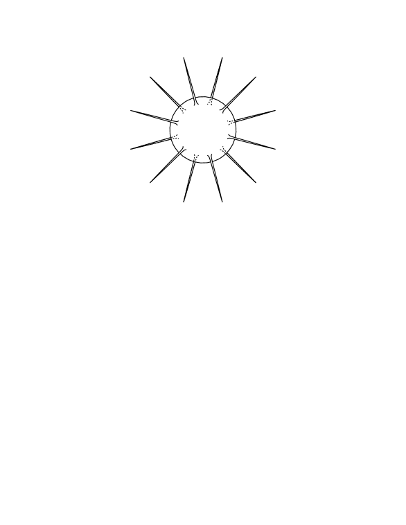
FIG. 1.: Classical membrane instability arises from spikes of infinitesimal area

If the spike is roughly cylindrical and has a radius $r$ and length $L$ then the energy is $2\pi rLT$. For a spike with very large $L$ but a small radius $r\ll 1/TL$ the energy cost is small but the spike is very long. This heuristic picture indicates that a quantum membrane will tend to have many fluctuations of this type, making it difficult to conceive of the membrane as an object which is well localized in space-time. Note that the quantum string theory does not have this problem since a long spike in a string always has energy proportional to the length of the string. In the matrix regularized version of the membrane theory, this instability appears as a set of flat directions in the classical theory. For example, if we have a pair of $N=2$ matrices with nonzero entries of the form

$$X^{1}=\left(\begin{array}[]{cc}x&0\\ 0&0\end{array}\right),\;\;\;\;\;X^{2}=\left(\begin{array}[]{cc}0&y\\ y&0\end{array}\right)$$ (55)

then a potential term ${\rm Tr}\;[X^{1},X^{2}]^{2}$ corresponds to a term proportional to $x^{2}y^{2}$. If either $x=0$ or $y=0$ then the other (nonzero) variable is unconstrained, giving flat directions in the moduli space of solutions to the classical equations of motion. This corresponds classically to a marginal instability in the matrix theory with $N>1$. (Note that in the previous section we distinguished matrices ${\bf X}^{i}$ from related functions $X^{i}$ by using bold font for matrices. We will henceforth drop this font distinction as long as the difference can easily be distinguished from context.)

In the quantum bosonic membrane theory, the apparent instability from the flat directions is cured because of the zero-modes of off-diagonal degrees of freedom. In the above example, for instance, if $x$ takes a large value then $y$ corresponds to a harmonic oscillator degree of freedom with a large mass. The zero point energy of this oscillator becomes larger as $x$ increases, giving an effective confining potential which removes the flat directions of the classical theory. This would seem to resolve the instability problem. Indeed, in the matrix regularized quantum bosonic membrane theory, there is a discrete spectrum of energy levels for the system of $N\times N$ matrices (Simon, 1983).

When we consider the supersymmetric theory, on the other hand, the problem returns. The zero point energies of the fermionic degrees of freedom conspire to precisely cancel the zero point energies of the bosonic oscillators. This cancellation gives rise to a continuous spectrum in the supersymmetric matrix theory. This result was proven by de Wit, Lüscher, and Nicolai (1989). They showed that for any $\epsilon>0$ and any energy $E\in[0,\infty)$ there exists a state $\psi$ in the $N=2$ maximally supersymmetric matrix model which is normalizable ($\int|\psi|^{2}=||\psi||^{2}=1$) and which has

$$||(H-E)\psi||^{2}<\epsilon.$$ (56)

This implies that the spectrum of the supersymmetric matrix quantum mechanics theory is continuous. This result indicated that it would not be possible to have a simple interpretation of the states of the theory in terms of a discrete particle spectrum. After this work there was little further development on the supersymmetric matrix quantum mechanics theory as a theory of membranes or gravity until almost a decade later.

B The BFSS conjecture

Motivated by recent work on D-branes and string dualities, Banks, Fischler, Shenker, and Susskind (1997) proposed that the large $N$ limit of the supersymmetric matrix quantum mechanics model described by Eq. (5) should describe all of M-theory in a light-front coordinate system. Although this conjecture fits neatly into the framework of the quantized membrane theory, the starting point of BFSS was to consider M-theory compactified on a circle $S^{1}$, with a large momentum in the compact direction. As discussed in Section I B, when M-theory is compactified on $S^{1}$ the resulting ten-dimensional theory is type IIA string theory. The quanta corresponding to momentum in the compact direction $x^{11}$ are the D0-branes of the IIA theory. In the “infinite momentum frame” of M-theory, where the momentum $p_{11}$ is taken to be very large, the dynamics of the theory becomes nonrelativistic (Weinberg, 1966; Kogut and Susskind, 1973). BFSS argued that this dynamics should be described by the large $N$ limit of a nonrelativistic system of D0-branes.

The low-energy Lagrangian for a system of $N$ type IIA D0-branes is the matrix quantum mechanics Lagrangian arising from the dimensional reduction to 0 + 1 dimensions of the 10D super Yang-Mills Lagrangian (Witten, 1996; see Polchinski, 1996 or Taylor, 1998 for a review)

$${\cal L}=\frac{1}{2gl_{s}}{\rm Tr}\;\left[\dot{X}^{a}\dot{X}^{a}+\frac{1}{2}[X^{a},X^{b}]^{2}+\theta^{T}(i\dot{\theta}-\Gamma_{a}[X^{a},\theta])\right]\,.$$ (57)

In this action the gauge has been fixed to $A_{0}=0$. Just as in Eq. (52), $X^{a}$ are 9 $N\times N$ bosonic matrices and $\theta$ are 16 Grassmann $N\times N$ matrices. Using the relations $R=g^{2/3}l_{11}=gl_{s}$ from Eq. (4), we see that in string units ($2\pi l_{s}^{2}=1$) we can replace $gl_{s}=R=2\pi l_{11}^{3}$. Thus, the Hamiltonian associated with Eq. (57) is in fact precisely equivalent to the matrix membrane Hamiltonian (52). This connection and its possible significance was first pointed out by Townsend (1996a). The fact that $l_{11}$ arises as the basic length scale in D0-brane quantum mechanics was discussed by Kabat and Pouliot (1996) and Douglas, Kabat, Pouliot, and Shenker (1997); this was an early indication that D0-branes might play a fundamental role as constituents of M-theory (see also Shenker, 1995, for a discussion of substring distance scales). The matrix theory Hamiltonian is often written, following BFSS, in the form

$$H = \frac{R}{2}{\rm Tr}\,\left(P^{i}P^{i}-{1\over 2}[X^{i},X^{j}][X^{i},X^{j}]+\theta^{T}\gamma_{i}[X^{i},\theta]\right)$$ (58)

where we have rescaled $X/g^{1/3}\rightarrow X$ and written the Hamiltonian in Planck units $l_{11}=1$. It is this Hamiltonian which BFSS conjectured should correspond with the infinite momentum limit of M-theory when $N\rightarrow\infty$.

The original BFSS conjecture was made in the context of the large $N$ theory. It was later argued by Susskind (1997a) that the finite $N$ matrix quantum mechanics theory should be equivalent to the discrete light-front quantized (DLCQ; see for example Pauli and Brodsky, 1985) sector of M-theory with $N$ units of compact momentum. We describe in section (III D) below an argument due to Seiberg and Sen which makes this connection more precise and which justifies the use of the low-energy D0-brane action in the BFSS conjecture.

While the BFSS conjecture was based on a different philosophy from that underlying the matrix quantization of the supermembrane theory we have discussed above, the fact that the M-theory membrane can be described as a classical configuration in the matrix quantum mechanics theory was a substantial piece of additional evidence given by BFSS for the validity of their conjecture. Two additional pieces of evidence were given by BFSS which extended their conjecture beyond the previous work on the matrix membrane theory.

One important point made by BFSS is that the Hilbert space of the matrix quantum mechanics theory naturally contains multiple particle states. This observation, which we discuss in more detail in the following subsection, resolves the problem of the continuous spectrum discussed above. Another piece of evidence given by BFSS for their conjecture is the fact that quantum effects in matrix theory give rise to long-range interactions between a pair of gravitational quanta (D0-branes). These interactions have precisely the structure expected from light-front supergravity. This result was first shown for D0-branes by a calculation of Douglas, Kabat, Pouliot, and Shenker (1997); we will discuss this result and its generalization to more general matrix theory interactions in Section IV.

C Matrix theory as a second-quantized theory

The classical equations of motion for a bosonic matrix configuration with the Hamiltonian (5) are (up to an overall constant)

$$\ddot{X}^{i}=-[[X^{i},X^{j}],X^{j}].$$ (59)

If we consider a block-diagonal set of matrices

$$X^{i}=\left(\begin{array}[]{cc}\hat{X}^{i}&0\\ 0&\tilde{X}^{i}\end{array}\right)$$ (60)

with first time derivatives $\dot{X}^{i}$ which are also of block-diagonal form, then the classical equations of motion for the blocks are separable

$$\ddot{\hat{X}}^{i}=-[[\hat{X}^{i},\hat{X}^{j}],\hat{X}^{j}],\;\;\;\;\;\;\;\;\;\;\ddot{\tilde{X}}^{i}=-[[\tilde{X}^{i},\tilde{X}^{j}],\tilde{X}^{j}]\,.$$ (61)

If we think of these blocks as describing two matrix theory objects with centers of mass

$$\hat{x}^{i}=\frac{1}{\hat{N}}{\rm Tr}\;\hat{X}^{i},\;\;\;\;\;\;\;\;\;\;\tilde{x}^{i}=\frac{1}{\tilde{N}}{\rm Tr}\;\tilde{X}^{i},$$ (62)

then we have two objects obeying classically independent equations of motion (See Fig. 2).

FIG. 2.: Two matrix theory objects described by block-diagonal matrices

It is straightforward to generalize this construction to a block-diagonal matrix configuration describing $k$ classically independent objects. This gives a simple indication of how matrix theory can encode, even in finite $N$ matrices, a configuration of multiple objects. In this sense it is natural to think of matrix theory as a second-quantized theory from the point of view of the target space.

Given the realization that matrix theory should describe a second quantized theory, the puzzle discussed above regarding the continuous spectrum of the theory is easily resolved. Assume that there is a state in matrix theory corresponding to a single graviton of M-theory with $H=0$, which is roughly a localized state (we will discuss such states in more detail in section V A). By taking two of these gravitons to have a large separation and a small relative velocity $v$ it should be possible to construct a two-body state with an arbitrarily small total energy using block diagonal matrices. Since the D0-branes of the IIA theory correspond to gravitons in M-theory with a single unit of longitudinal momentum, we therefore naturally expect to find a continuous spectrum of energies even in the theory with $N=2$. This resolves the puzzle found by de Wit, Lüscher, and Nicolai in a very pleasing fashion, and suggests that matrix theory is perhaps even more powerful than perturbative string theory, which only gives a first-quantized theory in the target space.

The second-quantized nature of matrix theory can also be seen heuristically in the continuous membrane theory. Recall that the instability of membrane theory appears in the classical theory of a continuous membrane when we consider the possibility of long thin spikes of negligible energy, as discussed in section III A. In a similar fashion, it is possible for a classical smooth membrane of fixed topology to be mapped to a configuration in the target space which looks like a system of multiple distinct macroscopic membranes connected by infinitesimal tubes of negligible energy (See Fig. 3).

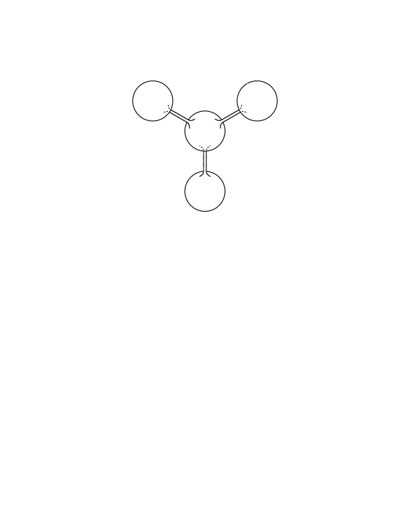
FIG. 3.: Membrane of fixed (spherical) topology mapped to multiple membranes connected by tubes in the target space

In the limit where the tubes become very small, their effect on the classical dynamics of the multiple membrane configuration becomes negligible, and we effectively have a system of multiple independent membranes moving in the target space. At the classical level, the sum of the genera of the membranes in the target space must be equal to or smaller than the genus of the single world-sheet membrane, but when quantum effects are included handles can be added to the membrane as well as removed. These considerations seem to indicate that any consistent quantum theory which contains a continuous membrane in its effective low-energy theory must contain configurations with arbitrary membrane topology and must therefore be a “second-quantized” theory from the point of view of the target space.

D Matrix theory and DLCQ M-theory

A theory which has been compactified on a lightlike circle can be viewed as a limit of a theory compactified on a spacelike circle where the size of the spacelike circle becomes vanishingly small in the limit. This point of view was used by Seiberg (1997b) and Sen (1998) to argue that light-front compactified M-theory is described through such a limiting process by the low-energy Lagrangian for many D0-branes, and hence by matrix theory. In this section we review this argument in detail. Other perspectives on the DLCQ limit are given in Balasubramanian, Gopakumar, and Larsen (1998) and de Alwis (1999). A nice synthesis of the various approaches to the matrix theory limit is given in Polchinski (1999).

Consider a space-time which has been compactified on a lightlike circle by identifying

$$\left(\begin{array}[]{c}x\\ t\end{array}\right)\sim\left(\begin{array}[]{c}x-R/\sqrt{2}\\ t+R/\sqrt{2}\end{array}\right)\,.$$ (63)

This theory has a quantized momentum in the compact direction $P^{+}=N/R$. The compactification (63) can be described as a limit of a family of spacelike compactifications

$$\left(\begin{array}[]{c}x\\ t\end{array}\right)\sim\left(\begin{array}[]{c}x-\sqrt{R^{2}/2+R_{s}^{2}}\\ t+R/\sqrt{2}\end{array}\right)$$ (64)

parameterized by the size $R_{s}\rightarrow 0$ of the spacelike circle, which is taken to vanish in the limit.

The system satisfying Eq. (64) is related to a system with the identification

$$\left(\begin{array}[]{c}x^{\prime}\\ t^{\prime}\end{array}\right)\sim\left(\begin{array}[]{c}x^{\prime}-R_{s}\\ t^{\prime}\end{array}\right)$$ (65)

through a boost with boost parameter $\beta$ given by

$$\beta=\frac{1}{\sqrt{1+\frac{2R_{s}^{2}}{R^{2}}}}\equiv 1-\frac{R_{s}^{2}}{R^{2}}.$$ (66)

We are interested in compactifying M-theory on a lightlike circle. This is related through the above limiting process to a family of spacelike compactifications of M-theory, which we know can be identified with the IIA string theory. At first glance, it may seem that the limit we are considering here is difficult to analyze from the IIA point of view. The IIA string coupling and string length are related to the compactification radius and 11D Planck length as in Eq. (4) by

$$g=(\frac{R_{s}}{l_{11}})^{3/2}, l_{s}^{2}\frac{l_{11}^{3}}{R_{s}}\,.$$ (67)

Thus, in the limit $R_{s}\rightarrow 0$ the string coupling $g$ becomes small as desired; the string length $l_{s}$, however, goes to $\infty$. Since $l_{s}^{2}=\alpha^{\prime}$, this corresponds to a limit of vanishing string tension. Such a limiting theory is very complicated and would not seem to provide a useful alternative description of the theory.

Let us consider, however, how the energy of the states we are interested in behaves in the class of limiting theories with spacelike compactification. If we want to describe the behavior of a state which has light-front energy $P^{-}$ and compact momentum $P^{+}=N/R$ then the spatial momentum in the theory with spatial $R_{s}$ compactification is $P^{\prime}=N/R_{s}$. The energy in the spatially compactified theory is

$$E^{\prime}=N/R_{s}+\Delta E,$$ (68)

where $\Delta E$ is at the energy scale we are interested in understanding. The term $N/R_{s}$ in the energy is simply the mass-energy of the $N$ D0-branes which correspond to the momentum in the compactified M-theory direction. Relating back to the near lightlike compactified theory we have

$$P^{-}=\frac{1}{\sqrt{2}}(E-P)=\frac{1}{\sqrt{2}}\frac{1+\beta}{\sqrt{1-\beta^{2}}}\Delta E\approx\frac{R}{R_{s}}\Delta E\,.$$ (69)

As a result we see that the energy $\Delta E$ of the IIA configuration needed to approximate the light-front energy $P^{-}$ is given by $\Delta E\approx P^{-}R_{s}/R$. We know that the string mass scale $1/l_{s}$ becomes small as $R_{s}\rightarrow 0$. We can compare the energy scale of interest to this string mass scale, however, and find

$$\frac{\Delta E}{(1/l_{s})}=\frac{P^{-}}{R}R_{s}l_{s}=\frac{P^{-}}{R}\sqrt{R_{s}l_{11}^{3}}\,.$$ (70)

This ratio vanishes in the limit $R_{s}\rightarrow 0$, which implies that although the string scale vanishes, the energy scale of interest is smaller still. Thus, it is reasonable to study the lightlike compactification through a limit of spatial compactifications in this fashion.

To make the correspondence between the light-front compactified theory and the spatially compactified limiting theories more transparent, we perform a change of units to a new Planck length $\tilde{l}_{11}$ in the spatially compactified theories in such a way that the energy of the states of interest is independent of $R_{s}$. For this condition to hold we must have

$$\Delta E\,\tilde{l}_{11}=P^{-}\frac{R_{s}{l}_{11}^{2}}{R\,\tilde{l}_{11}}$$ (71)

where $E,R$ and $P^{-}$ are independent of $R_{s}$ and all units have been explicitly included. This requires us to keep the quantity $R_{s}/\tilde{l}_{11}^{2}$ fixed in the limiting process. Thus, in the limit $\tilde{l}_{11}\rightarrow 0$.

We can summarize the preceding discussion as follows: to describe the sector of M-theory corresponding to light-front compactification on a circle of radius $R$ with light-front momentum $P^{+}=N/R$ we may consider the limit $R_{s}\rightarrow 0$ of a family of IIA configurations with $N$ D0-branes where the string coupling and string length

$$\tilde{g}=(R_{s}/\tilde{l}_{11})^{3/2}\rightarrow 0, \tilde{l}_{s}=\sqrt{\tilde{l}_{11}^{3}/R_{s}}\rightarrow 0$$ (72)

are defined in terms of a Planck length $\tilde{l}_{11}$ and compactification length $R_{s}$ which satisfy $R_{s}/\tilde{l}_{11}^{2}=R/l_{11}^{2}$. All transverse directions scale normally through $\tilde{x}^{i}/\tilde{l}_{11}=x^{i}/l_{11}$.

To give a very concrete example of how this limiting process works, let us consider a system with a single unit of longitudinal momentum $P^{+}=1/R$. We know that in the corresponding IIA theory, we have a single D0-brane whose Lagrangian has the relativistic Born-Infeld form

$${\cal L}=-\frac{1}{\tilde{g}\tilde{l}_{s}}\sqrt{1-\dot{\tilde{x}}^{i}\dot{\tilde{x}}^{i}}\,.$$ (73)

Expanding the square root we have

$${\cal L}=-\frac{1}{\tilde{g}\tilde{l}_{s}}\left(1-\frac{1}{2}\dot{\tilde{x}}^{i}\dot{\tilde{x}}^{i}+{\cal O}(\dot{\tilde{x}}^{4})\right).$$ (74)

Replacing $\tilde{g}\tilde{l}_{s}\rightarrow R_{s}$ and $\tilde{x}\rightarrow x\tilde{l}_{11}/l_{11}$ gives

$${\cal L}=-\frac{1}{R_{s}}+\frac{1}{2R}\dot{x}^{i}\dot{x}^{i}+{\cal O}(R_{s}/R).$$ (75)

Thus, we see that all the higher order terms in the Born-Infeld action vanish in the $R_{s}\rightarrow 0$ limit. The leading term is the D0-brane energy $1/R_{s}$ which we subtract to compare to the M-theory light-front energy $P^{-}$. Although we do not know the full form of the nonabelian Born-Infeld action describing $N$ D0-branes in IIA, it is clear that an analogous argument shows that all terms in this action other than those in the nonrelativistic supersymmetric matrix theory action (57) will vanish in the limit $R_{s}\rightarrow 0$.

This argument apparently demonstrates that matrix theory gives a complete description of the dynamics of DLCQ M-theory. There are several caveats which should be taken into account, however, with respect to this discussion. First, in order for this argument to be correct, it is necessary that there exists a well-defined theory with the properties expected of M-theory, and that there exist a well-defined IIA string theory which arises as the compactification of M-theory. Neither of these statements is at this point definitely established. Thus, this argument must be taken as contingent upon the definition of these theories. Second, although we know that 11D supergravity arises as the low-energy limit of M-theory, this argument does not necessarily indicate that matrix theory describes DLCQ supergravity in the low-energy limit. It may be that to make the connection to supergravity it is necessary to deal with subtleties of the large $N$ limit.

While there are reasons to suspect that care must be taken with this argument when $N$ becomes large, there are also some aspects of the story which become much clearer at large $N$. For large $N$, the rest energy $N/R_{s}$ from Eq. (68) becomes very large, and modifies the flat space-time geometry we have assumed in this discussion. As discussed in Hyun, Kiem and Shin (1998), Balasubramanian, Gopakumar, and Larsen (1998), Itzhaki, Maldacena, Sonnenschein, and Yankielowicz (1998), and Polchinski (1999), this back-reaction produces a “bubble” of eleven-dimensional space-time in the vicinity of the 0-branes, which in the large $N$ limit decompactifies the space-time. From the ten-dimensional point of view, this provides an explanation of how eleven-dimensional physics can be described by weakly coupled string theory in ten dimensions. The local gravitational effects of the D0-branes also have the effect of making the periodic dimension spacelike rather than lightlike, so that the problems of zero-modes usually associated with light-front field theories are avoided.

In the following sections we will discuss some more explicit approaches to connecting matrix theory with supergravity. In particular, we will see how far it is possible to go in demonstrating that 11D supergravity arises from calculations in the finite $N$ version of matrix theory, which is a completely well-defined theory.

IV Interactions in matrix theory

As we discussed in section III C, a many-body system is described in matrix theory by a set of block-diagonal matrices. Classically, the blocks describing each object evolve independently, so that there are no classical interactions in matrix theory between separated objects. How, then, can matrix theory be said to describe even classical gravitational interactions?

The answer to this question is quite remarkable, and is one of the most important features of this theory. It turns out that classical gravitational interactions arise through quantum loop effects in matrix theory. The first example of this classical-quantum correspondence was used as a piece of evidence for the validity of the 1996 matrix theory conjecture by BFSS. These authors pointed out that earlier work on D0-brane scattering in type IIA string theory by Douglas, Kabat, Pouliot, and Shenker (1997) gave a leading-order interaction between a pair of individual D0-branes which agrees precisely with the interaction between a pair of gravitons in eleven-dimensional supergravity according to the conjectured matrix theory correspondence. The interaction between the D0-branes in this calculation arises from a one-loop quantum mechanical calculation, while the leading interaction between gravitons in eleven dimensions is purely a classical effect arising from the linearized gravity theory. It was shown by Paban, Sethi, and Stern (1998a) that the leading one-loop interaction term in matrix theory is exact and is protected by a supersymmetric nonrenormalization theorem. A power counting argument (Becker, Becker, Polchinski, and Tseytlin, 1997) indicates that $n$th order nonlinear gravitational effects require $n$-loop interactions in the matrix quantum mechanics. This leads to the hypothesis that perhaps all classical gravitational interactions can be reproduced by perturbative calculations in matrix theory. At the linearized level this statement seems to be correct. It was shown by Kabat and Taylor (1998b) that all linearized gravitational interactions between a pair of bosonic sources can be reproduced by a general one-loop matrix theory calculation. Taylor and Van Raamsdonk (1999a) generalized this result to quadratic order in fermions. Beyond the linearized theory, however, this hypothesis is less strongly supported. There is evidence that some simple nonlinear gravitational interactions are correctly reproduced by perturbative calculations in matrix theory, including an impressive demonstration of agreement between three-graviton interactions and a two-loop calculation in $N=3$ matrix theory by Okawa and Yoneya (1999a, 1999b). It has also been argued by Dine, Echols, and Gray (2000), however, that terms arise in a three-loop matrix theory calculation which cannot correspond to third order gravitational effects. While some of the one-loop and two-loop interaction terms are protected by supersymmetric nonrenormalization theorems (Paban, Sethi, and Stern, 1998a, 1998b), there is no evidence that higher-loop effects are similarly constrained. Thus, even if the matrix theory conjecture is correct, it may not be possible to directly demonstrate the correspondence with supergravity by perturbative finite $N$ calculations in matrix quantum mechanics. In this section we describe the perturbative matrix theory calculations just discussed and the correspondence with supergravity interactions in some detail, as well as discussing the known supersymmetric nonrenormalization theorems and their consequences.

In subsection IV A we discuss perturbative calculations of two-body interactions in matrix theory. We begin by reviewing the perturbative Yang-Mills formalism in background field gauge, which can be used to carry out loop calculations in matrix theory. We describe in detail the one-loop calculation for a pair of D0-branes with relative velocity $v$. We then summarize the results of the one-loop calculation for a general two-body interaction and show that these interaction terms can be described by a sum of linearized supergravity interactions arising from the exchange of a single graviton, 3-form quantum or gravitino. We review results on spin effects and higher order terms for interactions between a pair of matrix theory gravitons, and we discuss nonrenormalization theorems and their implications for two-graviton interactions. In subsection IV B we discuss interactions between more than two objects. We discuss the N-body problem in general, and we review positive results for 3-graviton scattering and negative results for scattering of 4 or more gravitons. Section IV C contains a brief discussion of interactions involving longitudinal momentum transfer, which correspond to nonperturbative processes in matrix theory. In Subsection IV D we review the status of the correspondence between matrix theory and supergravity, and discuss possible subtleties in the large $N$ limit. We also briefly discuss work on reproducing quantum corrections to supergravity interactions from the matrix theory point of view. All the analysis in this section deals with matrix theory in a flat space-time background. Some progress towards understanding matrix theory in a curved space-time background is reviewed in Section VI B.

A Two-body interactions

1 The background field formalism

In this subsection we review the background formalism for Yang-Mills theory in the context of the (0+1)-dimensional matrix quantum mechanics theory. For a more complete introduction to the background field method, see for example Abbott (1981, 1982). Starting from the dimensionally reduced Yang-Mills action describing a system of $N$ D0-branes (without gauge-fixing $A$), the matrix theory Lagrangian is

$${\cal L}=\frac{1}{2R}{\rm Tr}\;\left[D_{0}X^{i}\;D_{0}X^{i}+\frac{1}{2}[X^{i},X^{j}]^{2}+\theta^{T}(i\dot{\theta}-\gamma_{i}[X^{i},\theta])\right]$$ (76)

where

$$D_{0}X^{i}=\partial_{t}X^{i}-i[A,X^{i}].$$ (77)

We wish to expand each of the matrix theory fields around a classical background. We will assume here for simplicity that the background has a vanishing gauge field and vanishing fermionic fields. The general situation with background fermionic fields as well as bosonic fields is described in Taylor and Van Raamsdonk (1999a). We expand the bosonic fields in terms of a background plus a fluctuation

$$X^{i} = B^{i}+Y^{i}.$$

We choose the background field gauge

$$D^{{\rm bg}}_{\mu}A^{\mu}=\partial_{t}A-i[B^{i},X^{i}]=0.$$ (78)

This gauge can be implemented by adding a term $-(D^{{\rm bg}}_{\mu}A^{\mu})^{2}$ to the action and including the appropriate ghosts. The nice feature of this gauge is that the terms quadratic in the bosonic fluctuations simplify considerably.

The complete gauge-fixed action including ghosts is written in Euclidean time $\tau=it$ as

$$S=S_{0}+S_{2}+S_{3}+S_{4}$$ (79)

where

$$S_{0} = \frac{1}{2R}\int d\tau{\rm Tr}\;\left[\partial_{\tau}B^{i}\partial_{\tau}B^{i}+\frac{1}{2}[B^{i},B^{j}]^{2}\right]$$ (80)

$$S_{2} = \frac{1}{2R}\int d\tau{\rm Tr}\;\left[\partial_{\tau}Y^{i}\partial_{\tau}Y^{i}-[B^{i},Y^{j}][B^{i},Y^{j}]-[B^{i},B^{j}][Y^{i},Y^{j}]\right.$$ (83)

$$\left.\hskip 57.81621pt+\partial_{\tau}A\partial_{\tau}A-[B^{i},A][B^{i},A]-2i\dot{B}^{i}[A,Y^{i}]\right.$$

$$\left.\hskip 57.81621pt+\partial_{\tau}\bar{C}\partial_{\tau}C-[B^{i},\bar{C}][B^{i},C]+\theta^{T}\dot{\theta}-\theta^{T}\gamma_{i}[B^{i},\theta]\right]$$

and where $S_{3}$ and $S_{4}$ contain terms cubic and quartic in the fluctuations $Y^{i},A,C,\theta$. These interaction terms are given explicitly in Becker and Becker (1997). Note that we have taken $A\rightarrow-iA$ as appropriate for the Euclidean formulation.

This gauge-fixed action can be used to perturbatively compute the effective action governing the interaction between any set of matrix theory objects. This effective action in turn determines the scattering phase shift of the objects in the eikonal approximation. In general, to calculate the effective interaction potential to arbitrary order it is necessary to include the terms $S_{3}$ and $S_{4}$ in the action. The propagators for each of the fields can be computed from the quadratic term $S_{2}$. A systematic diagrammatic expansion then yields the effective potential to arbitrarily high order. The only calculations which we describe in detail here are one-loop terms in the effective potential, for which the quadratic action $S=S_{0}+S_{2}$ is sufficient.

2 Two-graviton interactions at leading order

According to the BFSS conjecture, a $1\times 1$ matrix describing a single D0-brane in type IIA string theory corresponds to a graviton of M-theory with longitudinal momentum $p^{+}=1/N$. As we will discuss in further detail in section V A, at distances large compared to the size of the wavefunction describing the single graviton, it is sufficient to use a classical approximation $X^{i}=a^{i}+v^{i}t$ for the bosonic fields describing a single D0-brane moving along a linear trajectory in transverse 9-dimensional space with velocity $v^{i}$ and position $a^{i}$ at time $t=0$. Given this interpretation of a classical $1\times 1$ matrix, and the many-body interpretation of block-diagonal matrices described in III C, a classical background describing a pair of gravitons with relative velocity $v$ and impact parameter $b$ is given in the center of mass frame in the Euclidean theory by

$$B^{1}=\frac{-i}{2}\left(\begin{array}[]{cc}v\tau&0\\ 0&-v\tau\end{array}\right),\;\;\;\;\;B^{2}=\frac{1}{2}\left(\begin{array}[]{cc}b&0\\ 0&-b\end{array}\right),\;\;\;\;\;B^{i}=0,i>2\,.$$ (88)

In assuming this classical background we have ignored polarization effects, which are discussed in subsections IV A 5 and V A 2. Following Douglas, Kabat, Pouliot, and Shenker (1997), we can use the matrices (88) as a background and perform a one-loop calculation to find the leading long-range interaction between these two matrix theory gravitons. Related earlier calculations were performed by Bachas (1996) and Lifschytz (1996).

Inserting the background (88) into Eq. (83) we see that at a fixed value of time the Lagrangian at quadratic order for the 10 complex bosonic off-diagonal components of $A$ and $Y^{i}$ is that of a system of 10 harmonic oscillators with mass matrix

$$(\Omega_{b})^{2}=\left(\begin{array}[]{ccccc}r^{2}&-2iv&0&\cdots&0\\ 2iv&r^{2}&0&\ddots&0\\ 0&0&r^{2}&\ddots&\vdots\\ \vdots&\ddots&\ddots&\ddots&0\\ 0&0&\cdots&0&r^{2}\end{array}\right)$$ (89)

where $r^{2}=b^{2}+(vt)^{2}$ is the instantaneous separation between the gravitons. There are two complex off-diagonal ghosts with $\Omega^{2}=r^{2}$. There are 16 fermionic oscillators with a mass-squared matrix

$$(\Omega_{f})^{2}=r^{2}{\hbox to0.0pt{1\hss}\hskip 1.6pt\hbox{1}}_{16\times 16}+v\gamma_{1}\,.$$ (90)

To perform a completely general calculation of the two-body effective interaction potential to all orders in $1/r$ it is necessary to perform a diagrammatic expansion using the exact propagators for the bosonic and fermionic fields. For example, the bosonic propagator satisfying

$$(-\partial^{2}+b^{2}+v^{2}\tau^{2})\Delta_{B}(\tau,\tau^{\prime}|b^{2}+v^{2}\tau^{2})=\delta(\tau-\tau^{\prime})$$ (91)

is given by the expression (Becker and Becker, 1997)

$$\Delta_{B}(\tau,\tau^{\prime}|b^{2}+v^{2}\tau^{2}) = \int_{0}^{\infty}ds\;e^{-b^{2}s}\sqrt{\frac{v}{2\pi\sinh 2sv}}\,\exp\left(-\frac{v}{2\sinh 2sv}((\tau^{2}+\tau^{\prime 2})\cosh 2sv-2\tau\tau^{\prime})\right).$$ (92)

In general, even for a simple 2-graviton calculation there is a fair amount of algebra involved in extracting the effective potential using propagators of the form (92). If, however, we are only interested in calculating the leading term in the long-range interaction potential we can simplify the calculation by making the quasi-static assumption that all the oscillator frequencies $\omega$ of interest are large compared to the ratio $v/r$. In this approximation, all the oscillators stay in their ground state over the time of the interaction, so that the effective potential between the two objects is simply given by the sum of the ground-state energies of the boson, ghost and fermion oscillators

$$V_{{\rm qs}}=\sum_{b}\omega_{b}-\sum_{g}\omega_{g}-\frac{1}{2}\sum_{f}\omega_{f}.$$ (93)

(Note that the bosonic and ghost oscillators are complex so that no factor of 1/2 is included.)

In the situation of two-graviton scattering we can therefore calculate the effective potential by diagonalizing the frequency matrices $\Omega_{b},\Omega_{g}$, and $\Omega_{f}$. We find that the bosonic oscillators have frequencies

$$\omega_{b} = r\;\;\;\;\;{\rm with\ multiplicity\ 8}$$

$$\omega_{b} = \sqrt{r^{2}\pm 2v}\;\;\;\;\;{\rm with\ multiplicity\ 1\ each}.$$

The 2 ghosts have frequencies $\omega_{g}=r,$ and the 16 fermions have frequencies

$$\omega_{f}=\sqrt{r^{2}\pm v}\;\;\;\;\;{\rm with\ multiplicity\ 8\ each}.$$ (94)

The effective potential for a two-graviton system with instantaneous relative velocity $v$ and separation $r$ is thus given by the leading term in a $1/r$ expansion of the expression

$$V=\sqrt{r^{2}+2v}+\sqrt{r^{2}-2v}+6r-4\sqrt{r^{2}+v}+4\sqrt{r^{2}-v}.$$ (95)

Expanding in $v/r^{2}$ we see that the terms of order $r,v/r,v^{2}/r^{3}$ and $v^{3}/r^{5}$ all cancel. The leading term is

$$V=-\frac{15}{16}\frac{v^{4}}{r^{7}}+{\cal O}(\frac{v^{6}}{r^{11}})\,.$$ (96)

As mentioned above, this result agrees with the leading term in the effective potential between two gravitons with $P^{+}=1/R$ in light-front 11D supergravity. We will discuss the supergravity side of this calculation in more detail in the following section.

3 General two-body systems and linearized supergravity at leading order

We now generalize the background to include an arbitrary pair of bosonic matrix theory objects, described by block-diagonal matrices

$$B^{i}=\left(\begin{array}[]{cc}\hat{X}^{i}&0\\ 0&\tilde{X}^{i}\end{array}\right)$$ (97)

where $\hat{X}^{i}$ and $\tilde{X}^{i}$ are $\hat{N}\times\hat{N}$ and $\tilde{N}\times\tilde{N}$ matrices. The separation distance between the objects, which we will use as an expansion parameter, is given by

$$r^{i}=\frac{1}{\hat{N}}{\rm Tr}\;\hat{X}^{i}-\frac{1}{\tilde{N}}{\rm Tr}\;\tilde{X}^{i}\,.$$ (98)

To compute the leading term in the interaction potential, following Kabat and Taylor (1998b), we insert Eq. (97) into Eq. (83) and, as in the simpler two-graviton example, compute the frequency matrices for the bosons, ghosts, and fermions. We summarize here the results of this calculation. Expanding the frequency matrices as before in powers of $1/r$, and using Eq. (93), for a completely arbitrary pair of objects the potential again vanishes to order $1/r^{7}$. At this order the potential is

$$V_{\rm leading} = {\rm Tr}\,\left(\Omega_{b}\right)-{1\over 2}{\rm Tr}\,\left(\Omega_{f}\right)-2{\rm Tr}\,\left(\Omega_{g}\right)=-\frac{5}{128r^{7}}{\rm STr}\;{\cal F}$$ (99)

where

$${\cal F}=24F^{\mu}{}_{\nu}F^{\nu}{}_{\lambda}F^{\lambda}{}_{\sigma}F^{\sigma}{}_{\mu}-6F_{\mu\nu}F^{\mu\nu}F_{\lambda\sigma}F^{\lambda\sigma}$$ (100)

and ${\rm STr}$ indicates that the trace is symmetrized over all possible orderings of the $F$’s. The field strength $F_{\mu\nu}$ is a linear combination of contributions from each of the two objects

$$F_{\mu\nu}=\hat{F}_{\mu\nu}-\tilde{F}_{\mu\nu},$$ (101)

where $\hat{F}_{\mu\nu}$ and $\tilde{F}_{\mu\nu}$ are defined through

$$F_{0i}=\dot{X}^{i},\;\;\;\;\;\;\;\;\;\;F_{ij}=i[X^{i},X^{j}]$$ (102)

in terms of $\hat{X}$ and $\tilde{X}$ respectively.

Because of the linear structure of Eq. (101), it is possible to decompose the potential $V_{{\rm leading}}$ into a sum of terms which are written as products of a function of $\hat{X}$ and a function of $\tilde{X}$, where the terms can be grouped according to the number of Lorentz indices contracted between the two objects. With some algebra, this potential can be rewritten in the suggestive form

$$V_{\rm leading} = V_{\rm gravity}+V_{\rm electric}+V_{\rm magnetic}$$ (103)

$$V_{\rm gravity} = -{15R^{2}\over 4r^{7}}\left({\hat{\cal T}}^{IJ}{\tilde{\cal T}}_{IJ}-{1\over 9}{\hat{\cal T}}^{I}{}_{I}{\tilde{\cal T}}^{J}{}_{J}\right)$$ (104)

$$V_{\rm electric} = -{45R^{2}\over r^{7}}{\hat{\cal J}}^{IJK}{\tilde{\cal J}}_{IJK}$$ (105)

$$V_{\rm magnetic} = -{45R^{2}\over r^{7}}{\hat{\cal M}}^{+-ijkl}{\tilde{\cal M}}^{-+ijkl}\,.$$ (106)

This is, as we shall discuss shortly, precisely the form of the interactions we expect to see from 11D supergravity in light-front coordinates, where ${\cal T},{\cal J}$, and ${\cal M}$ play the role of the (integrated) stress tensor, membrane current, and M5-brane current of the two objects. The quantities appearing in this decomposition are defined as follows.

The matrix stress tensor ${\cal T}^{IJ}$ is a symmetric tensor with components

$${\cal T}^{--} = {1\over R}\;{\rm STr}\,\frac{{\cal F}}{96}$$ (107)

$${\cal T}^{-i} = {1\over R}\;{\rm STr}\,\left({1\over 2}{\dot{X}}^{i}{\dot{X}}^{j}{\dot{X}}^{j}+{1\over 4}{\dot{X}}^{i}F^{jk}F^{jk}+F^{ij}F^{jk}{\dot{X}}^{k}\right)$$ (108)

$${\cal T}^{+-} = {1\over R}\;{\rm STr}\,\left({1\over 2}{\dot{X}}^{i}{\dot{X}}^{i}+{1\over 4}F^{ij}F^{ij}\right)$$ (109)

$${\cal T}^{ij} = {1\over R}\;{\rm STr}\,\left({\dot{X}}^{i}{\dot{X}}^{j}+F^{ik}F^{kj}\right)$$ (110)

$${\cal T}^{+i} = {1\over R}\;{\rm STr}\,{\dot{X}}^{i}$$ (111)

$${\cal T}^{++} = {N\over R}\,.$$ (112)

The matrix membrane current ${\cal J}^{IJK}$ is a totally antisymmetric tensor with components

$${\cal J}^{-ij} = {1\over 6R}{\rm STr}\,\left({\dot{X}}^{i}{\dot{X}}^{k}F^{kj}-{\dot{X}}^{j}{\dot{X}}^{k}F^{ki}-{1\over 2}{\dot{X}}^{k}{\dot{X}}^{k}F^{ij}+{1\over 4}F^{ij}F^{kl}F^{kl}+F^{ik}F^{kl}F^{lj}\right)$$ (113)

$${\cal J}^{+-i} = {1\over 6R}{\rm STr}\,\left(F^{ij}{\dot{X}}^{j}\right)$$ (114)

$${\cal J}^{ijk} = -{1\over 6R}{\rm STr}\,\left({\dot{X}}^{i}F^{jk}+{\dot{X}}^{j}F^{ki}+{\dot{X}}^{k}F^{ij}\right)$$ (115)

$${\cal J}^{+ij} = -{1\over 6R}{\rm STr}\,F^{ij}\,.$$ (116)

Note that we retain some quantities — in particular ${\cal J}^{+-i}$ and ${\cal J}^{+ij}$ — which vanish at finite $N$ (by the Gauss constraint and antisymmetry of $F^{ij}$, respectively). These terms represent membrane charges which are only present in the large $N$ limit. We also define higher moments of these terms below which can be non-vanishing at finite $N$; the existence of these higher moments makes it useful to include these formally vanishing terms even at finite $N$.

The matrix M5-brane current ${\cal M}^{IJKLMN}$ is a totally antisymmetric tensor with

$${\cal M}^{+-ijkl}={1\over 12R}{\rm STr}\,\left(F^{ij}F^{kl}+F^{ik}F^{lj}+F^{il}F^{jk}\right)\,.$$ (117)

At finite $N$ this vanishes by the Jacobi identity, but we shall retain it for the reasons noted above. This term represents the charge of an M5-brane wrapped in the longitudinal ($X^{-}$) direction. The other components of ${\cal M}^{IJKLMN}$ do not appear in the Matrix potential. In principle, we expect another component of the M5-brane current, ${\cal M}^{-ijklm}$, to be well-defined. This term arises from a moving longitudinal M5-brane. This term does not appear in the two-body interaction formula because it would couple to the charge ${\cal M}^{+ijklm}$ of a transverse (unwrapped) M5-brane. As we discuss in V D, this charge is expected to vanish classically in matrix theory. The component ${\cal M}^{-ijklm}$ can, however, be determined from the conservation of the M5-brane current, and was shown by Van Raamsdonk (1999) to be given by

$${\cal M}^{-ijklm}=\frac{5}{4R}{\rm STr}\;\left(\dot{X}^{[i}F^{jk}F^{lm]}\right).$$ (118)

Let us now compare the interaction potential Eq. (103) with the leading long-range interaction between two objects in eleven-dimensional light-front compactified supergravity. The scalar propagator in eleven dimensions is

$${\kern 1.0pt\vbox{\hrule height=1.2pt\hbox{\vrule width=1.2pt\hskip 3.0pt\vbox{\vskip 6.0pt}\hskip 3.0pt\vrule width=0.6pt}\hrule height=0.6pt}\kern 1.0pt}{}^{-1}(x)={1\over 2\pi R}\sum_{n}\int{dk^{-}d^{\,9}k_{\perp}\over(2\pi)^{10}}{e^{-i{n\over R}x^{-}-ik^{-}x^{+}+ik_{\perp}\cdot x_{\perp}}\over 2{n\over R}k^{-}-k_{\perp}^{2}}$$ (119)

where $n$ counts the number of units of longitudinal momentum $k^{+}$. To compare the leading term in the long-distance potential with matrix theory we extract the $n=0$ term, corresponding to interactions mediated by exchange of a supergraviton with no longitudinal momentum,

$${\kern 1.0pt\vbox{\hrule height=1.2pt\hbox{\vrule width=1.2pt\hskip 3.0pt\vbox{\vskip 6.0pt}\hskip 3.0pt\vrule width=0.6pt}\hrule height=0.6pt}\kern 1.0pt}{}^{-1}(x-y)={1\over 2\pi R}\delta(x^{+}-y^{+}){-15\over 32\pi^{4}|x_{\perp}-y_{\perp}|^{7}}\,.$$ (120)

Note that the exchange of quanta with zero longitudinal momentum gives rise to interactions that are instantaneous in light-front time, as emphasized in Hellerman and Polchinski (1999). This is precisely the type of instantaneous interaction that arises at one loop in Matrix theory. Such action-at-a-distance potentials are allowed by the Galilean invariance manifest in the light-front formalism.

The graviton propagator can be written in terms of this scalar propagator as

$$D_{\rm graviton}^{IJ,KL}=2\kappa^{2}\left(\eta^{IK}\eta^{JL}+\eta^{IL}\eta^{JK}-{2\over 9}\eta^{IJ}\eta^{KL}\right){\kern 1.0pt\vbox{\hrule height=1.2pt\hbox{\vrule width=1.2pt\hskip 3.0pt\vbox{\vskip 6.0pt}\hskip 3.0pt\vrule width=0.6pt}\hrule height=0.6pt}\kern 1.0pt}{}^{-1}(x-y),$$ (121)

where $2\kappa^{2}=(2\pi)^{5}R^{3}$ in string units. The effective supergravity interaction between two objects having stress tensors $\hat{T}_{IJ}$ and $\tilde{T}_{KL}$ can then be expressed as

$$S=-{1\over 4}\int d^{11}xd^{11}y\,\,\hat{T}_{IJ}(x)D_{\rm graviton}^{IJ,KL}(x-y)\tilde{T}_{KL}(y)\,.$$ (122)

This interaction has a leading term of precisely the form Eq. (104) if we define ${\cal T}^{IJ}_{g}$ to be the integrated component of the stress tensor

$${\cal T}^{IJ}_{g}\equiv\int dx^{-}d^{\,9}x_{\perp}T^{IJ}(x).$$ (123)

It is straightforward to show in a similar fashion that Eqs. (105) and (106) are precisely the forms of the leading supergravity interaction mediated by 3-form exchange between membrane currents and M5-brane currents of a pair of objects.

In this section we have summarized the analysis of the leading two-body interaction potential between an arbitrary pair of bosonic matrix theory objects. This analysis was generalized to include all quadratic and some quartic terms in the fermionic matrices by Taylor and Van Raamsdonk (1999a). With the inclusion of fermions and the added assumption that the background fields satisfy the classical equations of motion, the general form of the leading matrix theory potential in Eq. (103) remains essentially unchanged, although the integrated matrix theory currents given by Eq. (107)-(117) acquire additional terms at quadratic and higher order in the fermions. Furthermore, with the inclusion of fermionic backgrounds, new interaction terms between fermionic sources appear which correspond to linearized gravitational interactions mediated by the gravitino. These interaction terms allow for the identification of the fermionic components of the matrix theory supercurrent.

The fact that Eq. (103) (and its generalization to include fermions) is exactly the form of the leading long-range supergravity interaction between a general pair of supercurrent sources implies that matrix theory correctly reproduces all leading order linearized supergravity interactions, and that the integrated stress tensor, membrane current, and M5-brane current of M-theory objects are encoded in the $N\times N$ matrix degrees of freedom of matrix theory through Eqs. (107)-(117). An alternative approach to finding the matrix theory stress tensor and membrane current is to compute the stress tensor and membrane current of the membrane from the continuous theory defined by the action (50) for the bosonic membrane in a general background. The matrix theory stress tensor and membrane current should then follow from the matrix-membrane correspondence given in Eq. (37). This calculation was performed in Kabat and Taylor (1998b) and Dasgupta, Nicolai, and Plefka (2000). It turns out that indeed the matrix definitions given above for the stress tensor and membrane current are compatible with the expressions for the analogous expressions for continuum membrane, including higher moment terms which we discuss in the next subsection. The matrix expressions are not uniquely determined by this correspondence, however. Additional terms appear in the matrix theory currents which depend upon the higher degree of sensitivity to operator ordering afforded by the matrix description. These terms, like the appearance of longitudinal M5-branes, seem to be examples of new physical properties which are mysteriously added to the system in the matrix regularization process, making the regularized theory in many ways richer than the initial continuous membrane theory would suggest.

4 General two-body interactions

In the previous subsections we have considered only the leading $1/r^{7}$ terms in the two-body interaction potential. In this subsection we discuss higher order terms in the interaction potential between a general pair of sources.

Let us begin by considering the series of subleading terms in the linearized supergravity potential between a general pair of sources arising from higher multipole moments of the supergravity currents for the two sources. Performing a Taylor series expansion around the origin for each of the two stress tensor sources in Eq. (122), for example, we find an infinite series of terms in the effective potential arising from linearized graviton exchange

$$V_{{\rm gravity}} = \sum_{m\leq n=0}^{\infty}-\frac{15R^{2}}{4\;r^{7}}\left[\frac{(-1)^{n-m}}{(n-m)!m!}{\hat{\cal T}}_{g}^{IJ(i_{1}i_{2}\cdots i_{n-m})}\left(\eta_{IK}\eta_{JL}-\frac{1}{9}\eta_{IJ}\eta_{KL}\right){\tilde{\cal T}}_{g}^{KL(j_{1}j_{2}\cdots j_{m})}\right.$$ (125)

$$\hskip 86.72377pt\left.\times\partial_{i_{1}}\partial_{i_{2}}\cdots\partial_{i_{n-m}}\partial_{j_{1}}\partial_{j_{2}}\cdots\partial_{j_{m}}(\frac{1}{r^{7}})\right].$$

where the moments of the stress tensor in the supergravity theory are defined through

$\displaystyle{\cal T}_{g}^{IJ(i_{1}i_{2}\cdots i_{n})}\equiv\int dx^{-}d^{\,9}x_{\perp}\left(T^{IJ}(x)x^{i_{1}}x^{i_{2}}\cdots x^{i_{n}}\right).$

Similar multipole interactions arise from the exchange of 3-form field quanta, generalizing the leading interaction terms given in Eqs. (105) and (106).

Let us now consider how higher-order terms of the form (125) can be reproduced by loop calculations in matrix theory. If we consider all possible Feynman diagrams which might contribute to higher-order terms, it is straightforward to demonstrate by power counting that the complete two-body potential can be written as a sum of terms of the form

$$V=\sum_{n,k,l,m,p,\alpha}V_{n,k,l,m,p,\alpha}R^{n-1}\frac{X^{l}D^{p}F^{k}\psi^{2m}}{r^{3n+2k+l+3m+p-4}}.$$ (126)

where $n$ counts the number of loops in the relevant diagrams and $\psi$ describes the fermionic background fields. Each $D$ either indicates a time derivative or a commutator with an $X$, as in $\psi[X,\psi]$. The summation over the index $\alpha$ indicates a sum over many possible index contractions for every combination of $F$’s, $X$’s, and $D$’s and $\Gamma$ matrices between the $\psi$’s.

For a completely general pair of objects, only terms in the one-loop effective action have been understood in terms of supergravity. At one-loop order, when the fields are taken on-shell by imposing the matrix theory equations of motion, all terms with $k+m+p<4$ which have been calculated vanish. All terms with $k+m+p=4$ which have been calculated have $m\geq p$ and can be written in the form

$$V_{1,4-m-p,l,m,p,\alpha}\frac{X^{l}F^{(4-m-p)}\psi^{2(m-p)}(\psi D\psi)^{p}}{r^{7+m-p+l}}.$$ (127)

In this expression, the grouping of $\psi$ terms indicates the contraction of spinor indices. The terms can be ordered in an arbitrary fashion when considered as $U(N)$ matrices, and each ordering is associated with a different index $\alpha$ and overall coefficient. The terms in Eq. (127) have been explicitly determined for $m<2$ in Taylor and Van Raamsdonk (1998a), Kabat and Taylor (1998b), and Taylor and Van Raamsdonk (1999a). These terms precisely correspond to linearized supergravitational interactions of the form of Eq. (125). We now briefly summarize some of the details of this correspondence.

Matrix multipole moments: Associated with each of the components of the integrated matrix theory supercurrents given in Eqs. (107)-(117) there is an infinite sequence of higher multipole moments. The bosonic parts of these multipole moments are formed by simply including $l$ extra matrices $X^{i}$ into the formula for a given supercurrent component, and symmetrizing over all possible orderings of the matrices $\dot{X}^{i},F^{ij}$, and $X^{i}$ inside the trace. For example, the higher multipole moments of the component ${\cal T}^{+-}$ of the matrix theory stress tensor are given by

$${\cal T}^{+-(i_{1}i_{2}\cdots i_{n})}={1\over R}{\rm STr}\;\left[\left({1\over 2}{\dot{X}}^{i}{\dot{X}}^{i}+{1\over 4}F^{ij}F^{ij}\right)X^{i_{1}}X^{i_{2}}\cdots X^{i_{n}}\right]\ ,$$ (128)

where ${\rm STr}$ denotes a symmetrized trace. In the one-loop matrix theory potential between a general pair of objects, these higher multipole moments appear in the long-range potential in precisely the form of Eq. (125) and its generalization for interactions mediated by 3-form and gravitino exchange. The simplest example of such an interaction is a term in the interaction potential Eq. (127) of the form $\hat{{\cal J}}^{ij}\tilde{{\cal T}}^{-i}r^{j}/r^{9}\sim F^{4}X/r^{8}$ which appears in the case of a graviton moving in the long-range gravitational field of a matrix theory object with angular momentum

$${\cal J}^{ij}={\cal T}^{+i(j)}-{\cal T}^{+j(i)}$$ (129)

where the first moment of the matrix theory stress tensor component ${\cal T}^{+i}$ is defined through

$${\cal T}^{+i(j)}=\frac{1}{R}{\rm Tr}\;\left(\dot{X}^{i}X^{j}\right)\,.$$ (130)

Matrix 6-brane current: At order $1/r^{8}$ new “dyonic” interaction terms describing higher-moment membrane-M5-brane and D0-brane-D6-brane interactions appear in addition to the interactions mentioned above (Dhar and Mandel 1998; Billó, Di Vecchia, Frau, Lerda, Russo, and Sciuto, 1998; Taylor and Van Raamsdonk 1999a). These interactions again are exactly in agreement with those of linearized supergravity, providing that we define (bosonic) components of a 6-brane current through

$${\cal S}^{+ijklmn}=\frac{1}{R}{\rm STr}\,\left(F_{[ij}F_{kl}F_{mn]}\right),\;\;\;\;\;\;\;\;\;\;{\cal S}^{ijklmnp}=\frac{7}{R}{\rm STr}\,\left(F_{[ij}F_{kl}F_{mn}\dot{X}_{p]}\right)\,.$$ (131)

It is interesting that this current appears in the matrix theory interaction potential, since the D6-brane of type IIA string theory corresponds to a Kaluza-Klein monopole descending from eleven dimensions, rather than an electrically or magnetically charged brane like the membrane or M5-brane (Townsend, 1995).

Fermion multipole moments: In addition to the purely bosonic components of the higher multipole moments, there are fermionic contributions. There are fermionic contributions to the integrated supercurrent components, as well as fundamentally fermionic contributions to higher moments of the supercurrent, where no derivatives act on the fermions. The simplest example of a term of the latter type is the spin contribution to the matrix theory angular momentum, first noted in the context of spinning gravitons by Kraus (1998).

$${\cal J}^{ij}_{{\rm fermion}}=\frac{1}{4R}{\rm Tr}\;\left(\psi\gamma^{ij}\psi\right)$$ (132)

Like the term in Eq. (130) above, this angular momentum term couples to the component ${\cal T}^{-i}\sim F^{3}$ of the matrix theory stress-energy tensor through terms of the form $\hat{{\cal J}}^{ij}\tilde{{\cal T}}^{-i}r^{j}/r^{9}$.

This summarizes all that is known about the two-body interaction for a completely general (and not necessarily supersymmetric) pair of matrix theory objects. All linearized supergravity interactions between an arbitrary pair of sources are reproduced by a one-loop matrix theory calculation up to quadratic order in fermions. No higher-loop calculations have been done for general backgrounds. It seems likely that the agreement between one-loop matrix theory calculations and linearized supergravity persists to higher order in the fermions, but the relevant contributions to the multipole moments of the supergravity currents have not yet been calculated for a general matrix theory object. It is quite plausible that the one-loop matrix theory interactions corresponding with linearized supergravity are all protected by supersymmetric nonrenormalization theorems, although this has not yet been demonstrated.

5 General two-graviton interactions

Aside from the general one-loop results described in the previous subsection, almost all other perturbative results on two-body interactions in matrix theory are for a pair of gravitons, which we discuss in this subsection. In the case of a pair of gravitons, the general interaction potential (126) simplifies to

$$V=\sum_{n,k,m}V_{n,k,m}R^{n-1}\frac{v^{k}\psi^{2m}}{r^{3n+2k+3m-4}}\,.$$ (133)

The leading terms for each value of $m\leq 4$ have been computed in the eikonal approximation using the one-loop approach, and are in agreement with the spin-spin interaction terms between gravitons in supergravity. The sum of these terms is summarized in Plefka, Serone, and Waldron (1998b), and is given by

$$V_{(1)} = -\frac{15}{16}\left[v^{4}+2v^{2}v_{i}D^{ij}\partial_{j}+2v_{i}v_{j}D^{ik}D^{jl}\partial_{k}\partial_{l}\right.$$ (135)

$$\left.\hskip 21.68121pt+\frac{4}{9}v_{i}D^{ij}D^{km}D^{lm}\partial_{j}\partial_{k}\partial_{l}+\frac{2}{63}D^{in}D^{jn}D^{km}D^{lm}\partial_{i}\partial_{j}\partial_{k}\partial_{l}\right]\frac{1}{r^{7}}$$

where $D^{ij}=\psi\gamma^{ij}\psi$. The term with a single $D$ proportional to $1/r^{8}$ arises from the spin angular momentum term described in Eq. (132).

No further checks have been made on the matrix theory/supergravity correspondence for terms with nontrivial fermion backgrounds. Simplifying to the spin-independent terms, the complete effective potential (133) simplifies still further to

$$V=\sum_{n,k}V_{n,k}R^{n-1}\frac{v^{k}}{r^{3n+2k-4}}.$$ (136)

Following Becker, Becker, Polchinski, and Tseytlin (1997), we write these terms in matrix form

$$\begin{array}[]{cccccccccc}V&=&\frac{1}{R}V_{0,2}\;v^{2}&&&&&&&\\ &&+&V_{1,4}\frac{v^{4}}{r^{7}}&+&V_{1,6}\frac{v^{6}}{r^{11}}&+&V_{1,8}\frac{v^{8}}{r^{15}}&+&\cdots\\ &&+&R\;V_{2,4}\;\frac{v^{4}}{r^{10}}&+&R\;V_{2,6}\;\frac{v^{6}}{r^{14}}&+&R\;V_{2,8}\;\frac{v^{8}}{r^{18}}&+&\cdots\\ &&+&R^{2}\;V_{3,4}\;\frac{v^{4}}{r^{13}}&+&R^{2}\;V_{3,6}\;\frac{v^{6}}{r^{17}}&+&R^{2}\;V_{3,8}\;\frac{v^{8}}{r^{21}}&+&\cdots\\ &&+&\vdots&+&\vdots&+&\vdots&+&\ddots\end{array}$$ (137)

where each row gives the contribution at fixed loop order. We will now give a brief review of what is known about these coefficients. First, let us note that in Planck units this potential is (restoring factors of $\alpha^{\prime}=l_{11}^{3}/R$ by dimensional analysis)

$$V=\sum_{n,k}V_{n,k}\frac{l_{11}^{3n+3k-6}}{R^{k-1}}\frac{v^{k}}{r^{3n+2k-4}}.$$ (138)

Since the gravitational coupling constant is $\kappa^{2}=2^{7}\pi^{8}l_{11}^{9},$ we only expect terms with $n+k\equiv 2\;({\rm mod}\;3)$ to correspond with classical supergravity interactions, since all terms in the classical theory have integral powers of $\kappa$. Of the terms explicitly shown in Eq. (137) only the diagonal terms satisfy this criterion. By including factors of $\hat{N}$ and $\tilde{N}$ for semi-classical graviton states with finite momentum $P^{+}$ and comparing to supergravity, one finds that the terms on the diagonal are precisely those which should correspond to classical supergravity. The terms beneath the diagonal have extra powers of $N$ for a fixed power of $v$ and would therefore dominate the diagonal terms in a fixed-$r$, large $N$ limit. It has been suggested that the terms above the diagonal correspond to quantum gravity corrections. It was shown by Becker, Becker, Polchinski, and Tseytlin (1997) that the sum of diagonal terms corresponding to the effective classical supergravity potential between two gravitons should be given by an expansion in $v^{2}$ of the potential

$$V_{{\rm classical}}=\frac{2r^{7}}{15R^{2}}\left(1-\sqrt{1-\frac{15R}{2}\frac{v^{2}}{r^{7}}}\right).$$ (139)

Now let us discuss the individual terms in Eq. (137). As we have discussed, the one-loop analysis gives a term $V_{1,4}=-15/16$, which agrees with linearized supergravity. The analysis of Section IV A 2 can be extended to the remaining one-loop terms. The next one-loop term vanishes $V_{1,6}=0$. Some efforts have been made to relate the higher order terms $V_{1,8},\ldots$ to quantum effects in 11D supergravity, but so far this interpretation is not clear. We briefly return to this question in Section IV D. The term $V_{2,4}=0$ was computed in Becker and Becker (1997). As expected, this term vanishes. The term $V_{2,6}=225/32$ was computed in Becker, Becker, Polchinski, and Tseytlin (1997). This term agrees with the expansion of Eq. (139). A general expression for the two-loop effective potential given by the second line of Eq. (137) was given in Becker and Becker (1998b), although there is no known connection between these terms and quantum corrections to supergravity.

It was argued by Paban, Sethi, and Stern (1998a, 1998b) that there can be no (below-diagonal) higher-loop corrections to the $v^{4}$ and $v^{6}$ terms on the diagonal. These authors considered the terms with the maximal number of fermions which are related to the $v^{4}$ and $v^{6}$ terms by supersymmetry. (For example, the $\psi^{8}/r^{11}$ term in Eq. (135) in the case $v^{4}$). They showed that these fermionic terms are uniquely determined by supersymmetry, and suggested that this in turn should uniquely fix the form of the bosonic terms proportional to $v^{4}$ and $v^{6}$. Explicit arguments along these lines for the nonrenormalization of the terms in Eq. (135) were given by Hyun, Kiem, and Shin (1999d), Okawa (1999), Nicolai and Plefka (2000), and Kazama and Muramatsu (2000). The results of these authors support the conclusion that all these terms are protected by supersymmetry, although the full supersymmetric off-shell action has not yet been constructed. The connection between the $v^{6}$ terms and the related terms with 12 fermions appears to be more subtle than in the $v^{4}$ case (Okawa, 1999), particularly when the action is taken off-shell. The nonrenormalization results for the $v^{4}$ and $v^{6}$ terms indicate that $V_{(n>1),4}=V_{(n>2),6}=0$. The existence of such nonrenormalization theorems in matrix theory was originally conjectured by BFSS in analogy to similar known theorems for higher-dimensional theories.

This completes our summary of what is known about interactions between two unpolarized gravitons in matrix theory. The complete set of known terms is given by

$$\begin{array}[]{ccccccccccc}V&=&\frac{1}{2R}v^{2}&&&&&&&&\\ &&&+&-\frac{15}{16}\frac{v^{4}}{r^{7}}&+&0&+&({\rm known})&\rightarrow&\\ &&&+&0&+&\frac{225}{32}R\frac{v^{6}}{r^{14}}&+&({\rm known})&\rightarrow&\\ &&&+&0&+&0&+&?&+&\cdots\\ &&&&\downarrow&&\downarrow&+&\vdots&+&\ddots\end{array}$$ (140)

It has been proposed that for arbitrary $N$ the analogues of the higher-loop diagonal terms should naturally take the form of a supersymmetric Born-Infeld type action (Chepelev and Tseytlin, 1998a, 1998b; Keski-Vakkuri and Kraus, 1998b; Balasubramanian, Gopakumar and Larsen, 1998). This would give rise in the case $N=2$ to a sum of the form Eq. (139). There is as yet, however, no proof of this statement beyond two loops. One particular obstacle to calculating the higher-loop terms in this series is that it is necessary to integrate over loops containing propagators of massless fields. These propagators can give rise to subtle infrared problems with the calculation. Some of these difficulties can be avoided by trying to reproduce higher-order supergravity interactions from interactions of more than two objects in matrix theory, the subject to which we turn in the next subsection. One interesting example of a two body interaction which has been considered at higher loop order involves the scattering of a D0-brane from a bound state of D0-branes and D6-branes. It was shown by Branco (1998) that the form of the $F^{6}$ term in the supersymmetric Born-Infeld action proposed by Chepelev and Tseytlin correctly reproduces the supergravity interaction in this situation. Dhar (1999) found, however, that the two-loop matrix theory calculation in this background suffers from divergences. It would be very interesting to understand whether indeed the higher terms in the nonabelian Born-Infeld action can be organized in such a way as to reproduce nonlinear gravitational effects between general sources.

B The N-body problem

So far we have seen that the linearized theory of supergravity is correctly reproduced by an infinite series of terms arising from one-loop calculations in matrix theory. We have also discussed 2-loop calculations of two-graviton interactions which agree with supergravity. If matrix theory is truly to reproduce all of classical supergravity, however, it must reproduce all the nonlinear effects of the fully covariant gravitational theory. The easiest way to study these nonlinearities is to consider N-body interaction processes. The first nonlinear gravitational effects appear at order $\kappa^{4}$ in the gravitational coupling. An example of such a nonlinear effect is the effect on a third object of the nonlinear contribution to the long-range gravitational field produced by the interaction of the fields from two distinct sources. This effect can be seen in classical gravity from a “Y”-shaped tree diagram connecting three separate objects. From the same dimensional analysis leading to Eq. (138), we expect these nonlinear effects to arise in a two-loop matrix theory calculation, and to have a leading term of the general form $v^{6}/r^{14}$, where the $v$’s are the velocities of the three bodies and the $r$’s are their relative positions. The simplest three-body interaction is that of three unpolarized gravitons, which can be described by the classical background

$$B^{i}=\left(\begin{array}[]{ccc}r_{1}^{i}+v_{1}^{i}&0&0\\ 0&r_{2}^{i}+v_{2}^{i}&0\\ 0&0&r_{3}^{i}+v_{3}^{i}\end{array}\right)\,.$$ (141)

Finding the leading terms in the two-loop effective action for an $N=3$ matrix configuration such as this is technically quite complicated. In an impressive pair of papers, Okawa and Yoneya (1999a, 1999b) carried out a complete perturbative calculation of all terms of order $v^{6}/r^{14}$ in the three-graviton effective action. (There are many such terms, which can be expressed as different functions of the relative velocities $v_{ij}=v_{i}-v_{j}$ and relative positions $r_{ij}=r_{i}-r_{j}$ of the three gravitons.) They found that there is an exact agreement between the two-loop matrix theory calculation and nonlinear corrections to supergravity at this order. Sethi and Stern (1999) have argued that, like the $v^{4}$ and $v^{6}$ terms in the $N=2$ theory, all these $v^{6}/r^{14}$ terms in the $N=3$ theory are protected from higher loop corrections by a supersymmetric nonrenormalization theorem.

One would naturally like to extend these results both by considering a general 3-body system, and by going beyond the 3-body problem to the general N-body problem. To date, however there has been very little progress on the problem of understanding higher order nonlinearities in the theory beyond those involved in the 3-graviton system. One foray into the general N-body calculation was made in Dine, Echols, and Gray (2000). These authors considered a subset of the terms in the general N-graviton interaction potential for arbitrary $N$. They found some terms at higher loop orders which agree with supergravity. They also identified terms, however, which appear in the 3-loop calculation of the 4-graviton effective action and which scale as $v^{6}/r^{17}$. These terms have improper scaling to correspond to supergravity terms, and are in fact “below the diagonal” as seen in Eq. (137). The appearance of such terms in the matrix theory perturbation series indicates a breakdown of the correspondence between perturbative matrix theory calculations and classical supergravity. This is the first concrete calculation where the two perturbative expansions have been shown to disagree. There are several subtleties in this calculation which may require further consideration before the case is completely closed. There are infrared divergences in this calculation which must be handled carefully, and which may lead to unexpected cancellations in some situations. There is also an issue of gauge choices; while the scattering S-matrix is gauge-independent, the effective action derived from Eq. (83) is gauge dependent. The manifest agreement discussed above between the one-loop matrix theory effective action and linearized supergravity seems to rely upon a fortuitous choice of gauge on both sides. If other gauges had been chosen, it might have been necessary to perform a complicated field redefinition to see the correspondence explicitly. It may be that for $N>2$ the background field gauge is not suitable for direct comparison to $N$-body interaction terms in the supergravity effective action. The issue of gauge-dependence was discussed in Hata and Moriyama (1999). As one goes to higher loop order it may also be necessary to understand recoil effects and the off-shell effective action; these issues are discussed in Periwal and von Unge (1998), Okawa and Yoneya (1998b), Okawa (1999), and Kazama and Muramatsu (2000). Despite these concerns, however, it seems most likely that this result is correct as stated, and that the correspondence between perturbative calculations in matrix theory and classical supergravity breaks down once high-order nonlinear effects are taken into consideration. As we will discuss in slightly more detail below, the nonrenormalization theorems which protect the one-loop and two-loop terms for $N\leq 3$ do not seem to extend to higher loops and larger values of $N$, so there is no contradiction between this breakdown of perturbative matrix theory and supersymmetry. It does, however, mean that we must work harder if we wish to demonstrate that classical eleven-dimensional supergravity is reproduced by matrix theory in the large $N$ limit.

C Longitudinal momentum transfer

In this section we have concentrated on interactions in matrix theory and supergravity where no longitudinal momentum is transferred from one object to another. A supergravity process in which longitudinal momentum is transferred from one object to another is described in the IIA theory by a process where one or more D0-branes are exchanged between coherent states consisting of clumps of D0-branes. Such processes are exponentially suppressed since the D0-branes are massive, and thus are not relevant for the expansion of the effective potential in terms of $1/r$ which we have been discussing. In the matrix theory picture, this type of exponentially suppressed process can only appear from nonperturbative effects. Clearly, however, for a full understanding of interactions in Matrix theory it will be necessary to study processes with longitudinal momentum transfer in detail and to show that they also correspond correctly with processes in supergravity and M-theory. Some progress has been made in this direction. Polchinski and Pouliot (1997) have calculated the scattering amplitude for two D2-branes for processes in which a D0-brane is transferred from one D2-brane to the other. In the Yang-Mills picture on the world-volume of the D2-branes, the incoming and outgoing configurations in this calculation are described in terms of an $U(2)$ gauge theory with a scalar field taking a VEV which separates the branes. The transfer of a D0-brane corresponds to an instanton-like process where a unit of flux is transferred from one brane to the other. The amplitude for this process was computed by Polchinski and Pouliot and shown to be in agreement with expectations from supergravity. This result suggests that processes involving longitudinal momentum transfer may be correctly described in Matrix theory. It should be noted, however, that the Polchinski-Pouliot calculation is not precisely a calculation of membrane scattering with longitudinal momentum transfer in Matrix theory since it is carried out in the D2-brane gauge theory language. In the T-dual Matrix theory picture the process in question corresponds to a scattering of D0-branes in a toroidally compactified space-time with the transfer of membrane charge. Processes with D0-brane transfer and the relationship between these processes and graviton scattering in matrix theory have been studied further in Dorey, Khoze, and Mattis (1997), Banks, Fischler, Seiberg, and Susskind (1997), Keski-Vakkuri and Kraus (1998d), Paban, Sethi, and Stern (1998c), Hyun, Kiem, and Shin (1999a), and de Boer, Hori, and Ooguri (1998).

D Summary and outlook for the matrix theory-supergravity correspondence

In this section we have described a variety of perturbative matrix theory calculations describing interactions between two or more “objects” described by blocks in a matrix theory background. For most of these calculations the perturbative results of matrix quantum mechanics precisely reproduce classical supergravity interactions between appropriate sources. It seems that all linearized supergravity interactions between arbitrary sources can be reproduced by a one-loop calculation in matrix theory. Some more specific nonlinear effects in supergravity, namely the second-order interactions in systems of two and three unpolarized gravitons, are also reproduced by two-loop matrix theory calculations. We have discussed supersymmetric nonrenormalization theorems which guarantee that the one-loop and two-loop graviton interaction calculations are protected by supersymmetry and cannot be corrected by higher-loop effects in matrix theory. While it has not been explicitly proven, it is tempting to believe that similar supersymmetric nonrenormalization theorems protect all the terms in the one-loop matrix theory effective action for any $N$, with backgrounds describing an arbitrary pair of interacting supergravity sources.

While it may be that all one-loop interactions and two-loop interactions for $N\leq 3$ are protected by supersymmetric nonrenormalization theorems as we have discussed, there is little evidence that higher-loop terms or two-loop terms for $N>3$ are protected by supersymmetry. Indeed, it was argued by Dine, Echols, and Gray (1998) that even in the $N=2$ theory terms of order $v^{8}$ and higher should experience higher loop corrections. Similarly, it was argued by Sethi and Stern (1999) that when $N>3$ even two-loop terms cannot be shown to be nonrenormalized using the same arguments as for one-loop terms and two-loop terms for small values of $N$. Given that the supersymmetric nonrenormalization theorems start to break down at this point, it is perhaps not surprising that Dine, Echols, and Gray (2000) found discrepancies between 3-loop calculations for $N=4$ and classical supergravity. If the correspondence does indeed break down at higher-loop order, then either we must accept that matrix theory does not successfully model M-theory, or there must be a more complicated way of understanding the correspondence between these theories. At this time there is not universal agreement as to how this question will eventually be resolved, but the only possible alternatives seem to be the following:

i) Matrix theory is correct in the large $N$ limit, and noncompact supergravity is reproduced by a naive large $N$ limit of the standard perturbative matrix theory calculations.

ii) Matrix theory is correct in the large $N$ limit, but to connect it with classical supergravity it is necessary to deal with subtleties in the large $N$ limit. (i.e., there are problems with the standard perturbative analysis at higher order)

iii) Matrix theory is simply wrong, and further terms need to be added to the dimensionally reduced super Yang-Mills action to find agreement with M-theory even in the large $N$ limit.

Let us review the evidence:

$\bullet$ Assuming that the result of Dine, Echols, and Gray is correct, and has been correctly interpreted, clearly (i) is not possible. The fact that the methods of Paban, Sethi, and Stern for proving nonrenormalization theorems in the $SU(2)$ theory break down for $SU(3)$ at two loops and at higher loop order also hints that (i) may not be correct.

$\bullet$ The analysis of Seiberg and Sen seems to indicate that either possibility (i) or (ii) should hold.

It seems that (ii) is the most likely possibility, given this limited evidence. There are several issues which are extremely important in understanding how this problem will be resolved. The first is the issue of Lorentz invariance. If a theory contains linearized gravity and is Lorentz invariant, then it is well known that it must be either the complete generally covariant gravity theory or just the pure linearized theory. Since we know that matrix theory has some nontrivial nonlinear structure which reproduces part of the nonlinearity of supergravity, it would seem that the conjecture must be valid if and only if the theory is Lorentz invariant. Unfortunately, so far there is no complete understanding of whether the quantum theory is Lorentz invariant (classical Lorentz invariance was demonstrated in de Wit, Marquard, and Nicolai, 1990). It was suggested in Lowe (1998) that the problems found in Dine, Echols, and Gray (2000) might be related to a breakdown of Lorentz invariance and that in fact extra terms must be added to the theory to restore this invariance; this would lead to possibility (iii) above.

Another critical issue in understanding how the perturbative matrix theory calculations should be interpreted is the issue of the order of limits. In the perturbative calculations discussed here we have assumed that the longitudinal momentum parameter $N$ is fixed for each of the objects we are taking as a background, and we have then taken the limit of large separations between each of the objects. Since the size of the wavefunction describing a given matrix theory object will depend on $N$ but not on the separation from a distant object, this gives a systematic approximation scheme in which the bound state and wavefunction effects for each of the bodies can be ignored in the perturbative analysis. If we really are interested in the large $N$ theory, however, the correct order of limits to take is the opposite. We should fix a separation distance $r$ and then take the large $N$ limit. Unfortunately, in this limit we have no systematic approximation scheme. The wavefunctions for the separate objects overlap significantly as the size of the objects grows. Indeed, it was argued recently by Polchinski (1999) that the size of the bound state wavefunction of $N$ D0-branes will grow at least as fast as $N^{1/3}$. As emphasized by Susskind (1999), this overlap of wavefunctions makes the theory very difficult to analyze. Indeed, if possibility (ii) above is correct, it may be very difficult to use matrix theory to reproduce all the nonlinear structure of classical supergravity, let alone to derive new results about quantum supergravity. On the other hand, it may be that whatever mechanism allows the one-loop and two-loop matrix theory results to correctly reproduce the first few terms in supergravity and to evade the problem of wavefunction overlap may persist at higher orders through a more subtle mechanism than those currently understood. Indeed, one of the must important outstanding questions regarding matrix theory is to understand precisely which terms in the naive perturbative expansion of the quantum mechanics will agree with classical supergravity, and more importantly, why these terms agree.

In this section we have focused on the problem of deriving classical eleven-dimensional supergravity from matrix theory. A very interesting, but more difficult, question is whether matrix theory can also successfully reproduce string/M-theory corrections to classical supergravity. The first such corrections would be ${\cal R}^{4}$ corrections to the Einstein-Hilbert action (Fradkin and Tseytlin, 1983). It was argued by Susskind (1997b) and Berglund and Minic (1997) that such terms should be reproduced by the $v^{8}/r^{18}$ terms which arise in the two-loop effective potential (137). It was shown by Keski-Vakkuri and Kraus (1998c) and Becker and Becker (1998a) that in a two-body interaction between a pair of gravitons with longitudinal momentum $N/R$ this term has the wrong scaling in $N$. This discrepancy was sharpened by Helling, Plefka, Serone, and Waldron (1999), who performed a two-loop calculation in a three-graviton background, and showed that the tensor structure of the $v^{8}/r^{18}$ terms disagrees with that expected from a ${\cal R}^{4}$ correction to gravity. While more work needs to be done in this direction, the results of these authors indicate that the perturbative loop expansion in matrix theory probably does not correctly reproduce quantum effects in M-theory. The most likely explanation for this discrepancy is that, like the higher-loop diagonal terms discussed above, such terms are not subject to nonrenormalization theorems, and are only reproduced in the large $N$ limit if the matrix theory conjecture is correct.

V M-theory objects from matrix theory

In this section we discuss how the matrix theory degrees of freedom can be used to construct the various objects of M-theory: the supergraviton, supermembrane, and M5-brane. We discuss classical and quantum supergravitons in matrix theory in subsection V A. We present a general discussion of the structure of extended objects and their charges in subsection V B, following which we discuss the matrix constructions of membranes and M5-branes in subsections V C and V D, respectively.

A Supergravitons

In DLCQ M-theory, for every integer $N$ there should be a localized state corresponding to a longitudinal graviton with $p^{+}=N/R$ and arbitrary transverse momentum $p^{i}$. We expect from the massless condition $m^{2}=-p^{I}p_{I}=0$ that such an object will have matrix theory energy $E=p_{i}^{2}/2p^{+}$. We discuss such states first classically and then in the quantum theory.

1 Classical supergravitons

The classical matrix theory potential is $-[X^{i},X^{j}]^{2}$, from which we have the classical equations of motion

$$\ddot{X}^{i}=-[[X^{i},X^{j}],X^{j}].$$ (142)

One simple class of solutions to these equations of motion can be found when the matrices minimize the potential at all times and therefore all commute. Such solutions are of the form

$$X^{i}=\left(\begin{array}[]{cccc}x^{i}_{1}+v^{i}_{1}t&0&0&\ddots\\ 0&x^{i}_{2}+v^{i}_{2}t&\ddots&0\\ 0&\ddots&\ddots&0\\ \ddots&0&0&x^{i}_{N}+v^{i}_{N}t\end{array}\right)\,.$$ (143)

This corresponds to a classical $N$-graviton solution, where each graviton has

$$p_{a}^{+}=1/R,\;\;\;\;\;p^{i}_{a}=v^{i}_{a}/R,\;\;\;\;\;E_{a}=v_{a}^{2}/(2R)=(p_{a}^{i})^{2}/2p^{+}\,.$$ (144)

A single classical graviton with $p^{+}=N/R$ can be formed by setting

$$x_{1}^{i}=\cdots=x_{N}^{i},\;\;\;\;\;v_{1}^{i}=\cdots=v_{N}^{i}$$ (145)

so that the trajectories of all the components are identical. This simple model for gravitons was used in all the spin-independent matrix theory calculations described in the previous section.

The classical graviton gives a simple example with which to understand the matrix theory stress tensor (107). The integrated stress tensor of a graviton can be written in the form

$${\cal T}^{IJ}=\frac{p^{I}p^{J}}{p^{+}},$$ (146)

where

$$p^{+}=N/R,\;\;\;\;\;p^{i}=p^{+}\dot{x}^{i},\;\;\;\;\;p^{-}=p_{\perp}^{2}/2p^{+}\,.$$ (147)

These expressions agree precisely with the matrix expressions for the stress tensor (107) using the matrices (143) with Eq. (145).

2 Quantum supergravitons

The picture of a supergraviton in quantum matrix theory is somewhat more subtle than the simple classical picture just discussed. Let us first consider the case of a single supergraviton with $p^{+}=1/R$. This corresponds to the U(1) case of the super Yang-Mills quantum mechanics theory. The Hamiltonian is simply

$$H=\frac{1}{2R}\dot{X}^{2},$$ (148)

since all commutators vanish in this theory. The bosonic part of the theory is simply a free nonrelativistic particle. In the fermionic sector there are 16 spinor variables with anticommutation relations $\{\theta_{\alpha},\theta_{\beta}\}=\delta_{\alpha\beta}$. By using the standard trick of writing these as 8 fermion creation and annihilation operators

$$\theta_{i}^{\pm}=\frac{1}{\sqrt{2}}(\theta_{i}\pm\theta_{i+8}),\;\;\;\;\;\;1\leq i\leq 8,$$ (149)

we see that the Hilbert space for the fermions is a standard fermion Fock space of dimension $2^{8}=256$. Indeed, this is precisely the number of states needed to represent all the polarization states of the graviton (44), the antisymmetric 3-tensor field (84), and the gravitino (128). For details of how the polarization states are represented in terms of the fermionic Fock space, see de Wit, Hoppe and Nicolai (1988), Plefka and Waldron (1998), Morales, Scrucca, and Serone (1998b), and Millar, Taylor, and Van Raamsdonk (2000).

The case when $N>1$ is much more subtle. We can factor out the overall $U(1)$ so that every state in the $SU(N)$ quantum mechanics theory has 256 corresponding states in the full theory. For the matrix theory conjecture to be correct, as BFSS pointed out, it should then be the case that for every $N$ there exists a unique threshold bound state in the $SU(N)$ theory with $H=0$. As mentioned before, no definitive answer as to the existence of such a state was given in the early work on matrix theory. The existence of a unique ground state for the matrix quantum mechanics can be demonstrated by showing both that the Witten index of the system is equal to one, and that there are no fermionic ground states. The first of these statements was finally proven for $N=2$ in Sethi and Stern (1998), demonstrating that at least one threshold bound state exists. These authors showed that the Witten index breaks up into a bulk and a boundary contribution, each of which is separately fractional. The uniqueness of the bound state for SU(2) was shown in Sethi and Stern (2000a). The existence of a bound state for $N>2$ was demonstrated when Moore, Nekrasov, and Shatashvili (2000) computed the bulk contribution to the index for general $N$ and Green and Gutperle (1998) computed the corresponding boundary contribution. (This boundary contribution has also been checked by numerical methods in Krauth and Staudacher, 1998.) Related work was done by Yi (1997), Porrati and Rozenberg (1998), and Konechny (1998). The Witten index for groups other than SU(N) was determined in Kac and Smilga (2000), Hanany, Kol, and Rajaraman (1999), and Staudacher (2000), where a puzzling discrepancy between the predictions of different methods was noted for the exceptional group $G_{2}$.

The exact determination of the bound state wavefunction, even for $N=2$, is a difficult problem on which little progress has been made. A more tractable and still very interesting problem is the determination of the asymptotic form of the ground state. It was shown by Sethi and Stern (2000a) that for the SU(2) theory the asymptotic form of the wavefunction is invariant under the SO(9) R-symmetry group of the quantum mechanics theory. Combining this with the conditions of integrability and SU(2) invariance are sufficient to uniquely fix the asymptotic form of the SU(2) wavefunction. Halpern and Schwartz (1998) used a second order Born-Oppenheimer approach to determine the form of the asymptotic wavefunction in the $SU(2)$ theory. This asymptotic form was reproduced using a first-order approach (based on the supersymmetry generators rather than the Hamiltonian) by Graf and Hoppe (1998) and Fröhlich, Graf, Hasler, Hoppe, and Yau (2000). It was shown by Bordemann, Hoppe, and Suter (1999) that the analogous condition of R-symmetry invariance is not sufficient to uniquely determine the asymptotics of the ground state for $N>2$. The extra information needed to determine the asymptotic form of the $SU(3)$ ground state was, however, described in Hoppe (1999) and the asymptotic form was found in Hoppe and Plefka (2000).

While little progress has been made so far towards an exact analytic description of the bound state wavefunction of two D0-branes, Sethi and Stern (2000b) considered the related problem of the bound state wavefunction of a D0-brane and a D4-brane. They found a system of equations describing this bound state and arrived at the surprising conclusion that the unique normalizable bound state could be described by a single equation in terms of a single unknown function. This extraordinary simplification hints that perhaps there is some hidden structure even in the case of two D0-branes which might eventually allow for an analytic description of the graviton bound state.

As discussed in IV D, to understand interactions between matrix theory gravitons in the large $N$ limit, it is crucial to understand how the size of the bound state wavefunction grows with $N$. With the limited information we have at this time about the wavefunctions for small values of $N$, it is difficult to rigorously determine the asymptotics as $N$ becomes large. It was argued by Nekrasov (1999) that the ground state wavefunction has a size which scales as $N^{1/3}$, saturating the lower bound found by Polchinski (1999). How such large wavefunctions interact when scattered at an impact parameter which is fixed as $N$ becomes large is a puzzle which must be better understood if we are to develop a deeper understanding of matrix theory as a model of quantum gravity.

B Extended objects from matrices

We have discussed the construction of localized graviton states as classical and quantum matrix theory configurations. In addition to these pointlike objects, we would like to construct M-theory membranes and M5-branes from the fundamental matrix degrees of freedom. These will be objects extended in one, two, and four spatial dimensions. In this subsection we make some general comments about the structure of these extended objects in matrix theory.

Let us begin by discussing the charges associated with the extended objects in matrix theory. In IV A 3 we used the correspondence between one-loop matrix theory interactions and linearized supergravity to construct an integrated stress tensor, membrane current and M5-brane current for a general matrix theory configuration. The components of these tensors with a $+$ index correspond to conserved charges in the theory. The components ${\cal T}^{++}$ and ${\cal T}^{+i}$ of the matrix stress tensor correspond to longitudinal and transverse momentum $N/R$ and $p^{i}$ respectively. The components ${\cal J}^{+-i}$ and ${\cal J}^{+ij}$ of the membrane current correspond to charges for membranes which are wrapped and unwrapped in the longitudinal direction, and the component ${\cal M}^{+-ijkl}$ of the M5-brane current corresponds to a charge for wrapped (longitudinal) M5-branes. No charge associated with unwrapped (transverse) M5-branes appears in the one-loop matrix theory interaction potential. The charges associated with extended objects all vanish at finite $N$; this corresponds physically to the fact that any finite-size configuration of membranes and M5-branes must have net charges which vanish, as all the branes must be compact.

An alternative understanding of the conserved charges associated with extended objects in matrix theory follows from the supersymmetry algebra of the theory. The eleven-dimensional supersymmetry algebra takes the form

$$\{Q_{\alpha},Q_{\beta}\}\sim P^{I}(\gamma_{I})_{\alpha\beta}+Z^{I_{1}I_{2}}(\gamma_{I_{1}I_{2}})_{\alpha\beta}+Z^{I_{1}\ldots I_{5}}(\gamma_{I_{1}\ldots I_{5}})_{\alpha\beta}$$ (150)

where the central terms $Z^{I_{1}I_{2}},Z^{I_{1}\ldots I_{5}}$ correspond to 2-brane and M5-brane charges. The supersymmetry algebra of Matrix theory was explicitly computed by Banks, Seiberg, and Shenker (1997). The full supersymmetry algebra of the theory takes the schematic form

$$\{Q,Q\}\sim P^{I}+z^{i}+z^{ij}+z^{ijkl},$$ (151)

as we would expect for the light-front supersymmetry algebra corresponding to Eq. (150). The charge

$$z^{i}\sim{\cal J}^{+-i}\sim i{\rm Tr}\;\left(\{P^{j},[X^{i},X^{j}]\}+{}[{}[X^{i},\theta^{\alpha}],\theta^{\alpha}]\right)$$ (152)

corresponds to longitudinal membranes (strings), the charge

$$z^{ij}\sim{\cal J}^{+ij}\sim-i{\rm Tr}\;[X^{i},X^{j}]$$ (153)

corresponds to transverse membranes and

$$z^{ijkl}\sim{\cal M}^{+-ijkl}\sim{\rm Tr}\;X^{[i}X^{j}X^{k}X^{l]}$$ (154)

corresponds to longitudinal M5-brane charge.

Yet another way to motivate these charge identifications is through T-duality in the type IIA picture. This approach is described in Taylor (1998, 2000), Taylor and Van Raamsdonk (1999a), and Myers (1999).

The perturbative matrix theory calculations described in IV A determine not only the conserved charges of the theory, but also the higher multipole moments of these charges. For example the multipole moments of the membrane charge $z^{ij}=-2\pi i{\rm Tr}\;[X^{i},X^{j}]$ can be written in terms of the matrix moments

$$z^{ij(k_{1}\cdots k_{n})}=-2\pi i\;{\rm STr}\;\left([X^{i},X^{j}]X^{k_{1}}\cdots X^{k_{n}}\right),$$ (155)

which are the matrix analogues of the moments

$$\int d^{2}\sigma\;\{X^{i},X^{j}\}X^{k_{1}}\cdots X^{k_{n}}$$ (156)

for the continuous membrane. The symbol ${\rm STr}$ as usual indicates a symmetrized trace, wherein the trace is averaged over all possible orderings of the terms $[X^{i},X^{j}]$ and $X^{k_{\nu}}$ appearing inside the trace. This corresponds to a particular ordering prescription in applying the matrix-membrane correspondence to Eq. (156). There is no a priori justification for this ordering prescription, but it is a consequence of the explicit calculations of interactions between general matrix theory objects described above. The same prescription can be used to define the multipole moments of the longitudinal membrane and M5-brane charges. These multipole moments can also be derived from T-duality arguments in type IIA, as in Taylor and Van Raamsdonk (1999b) and Myers (1999), but the ordering information implied by the symmetrized trace cannot be determined in this fashion.

Although as we have mentioned, the conserved charges in matrix theory corresponding to extended objects all vanish at finite $N$, the same is not true of the higher moments of these charges. As we will discuss in the following sections, it is possible to construct compact membrane and M5-brane configurations in matrix theory whose multipole moments of membrane and M5-brane charge are nonvanishing and agree to within terms of order $1/N^{2}$ with the continuous versions of these multipole moments. Conversely, by calculating the multipole moments of a fixed matrix configuration we can essentially reproduce the complete spatial dependence of the matter configuration to which the matrices correspond.

It is interesting to note that while the superalgebra in Eq. (151) does not contain a 6-brane charge, such a charge does appear in the one-loop matrix theory effective action, associated with dyonic interactions between D6-branes and D0-branes. The construction of 6-branes from multiple D0-branes was discussed in Taylor (1997b).

C Membranes

In this section we discuss the construction of M-theory membranes in terms of the matrix quantum mechanics degrees of freedom. It is clear from the derivation of matrix theory as a regularized supermembrane theory that there must be matrix configurations which in the large $N$ limit give arbitrarily good descriptions of any membrane configuration. It is somewhat instructive, however, to study some aspects of the geometry of simple matrix membranes at finite $N$. In subsection V C 1 we describe some explicit examples of compact membrane configurations and discuss how membrane geometry is encoded in a system of finite-size matrices. In subsection V C 2 we discuss noncompact matrix membranes, and in subsection V C 3 we discuss wrapped membranes, which appear as string excitations in matrix theory.

1 Compact membranes

One extremely simple example of a membrane configuration, which makes it clear that a smooth membrane geometry can be approximated quite well even at finite $N$ by simple matrix configurations, is the symmetric spherical membrane (Kabat and Taylor, 1997a). Imagine that we wish to construct a membrane embedded in an isotropic sphere $x_{1}^{2}+x_{2}^{2}+x_{3}^{2}=r^{2}$ in the first three dimensions of ${\mathbb{R}}^{11}$. The embedding functions for such a continuous membrane can be written as linear functions $X^{i}=r\xi^{i},1\leq i\leq 3,$ of the three Euclidean coordinates $\xi^{i}$ on the spherical world-volume. Using the matrix-membrane correspondence (37) we see that the matrix approximation to this membrane will be given by the $N\times N$ matrices

$$X^{i}=\frac{2r}{N}J^{i}\;\;\;\;\;\;1\leq i\leq 3$$ (157)

where $J^{i}$ are the generators of $SU(2)$ in the $N$-dimensional representation.

It is interesting to see how many of the geometrical and physical properties of the sphere can be extracted from the algebraic structure of these matrices, even for small values of $N$. We list here some of these properties.

i) Spherical locus: The matrices Eq. (157) satisfy

$$X_{1}^{2}+X_{2}^{2}+X_{3}^{2}=\frac{4r^{2}}{N^{2}}C_{2}(N){\hbox to0.0pt{1\hss}\hskip 1.6pt\hbox{1}}=r^{2}(1-1/N^{2}){\hbox to0.0pt{1\hss}\hskip 1.6pt\hbox{1}},$$ (158)

where $C_{2}(N)=(N^{2}-1)/4$ is the quadratic Casimir of $SU(2)$ in the $N$-dimensional representation. This shows that the D0-branes are in a noncommutative sense “localized” on a sphere of radius $r+{\cal O}(1/N^{2})$.

ii) Rotational invariance: The matrices Eq. (157) satisfy

$$R_{ij}X_{j}=U(R)\cdot X_{i}\cdot U(R^{-1}),$$ (159)

where $R\in SO(3)$ and $U(R)$ is the $N$-dimensional representation of $R$. Thus, the spherical matrix configuration is rotationally invariant up to a gauge transformation, even though the smooth membrane sphere has been “discretized” to a finite number of degrees of freedom.

iii) Spectrum: The matrix $X^{3}=2r{\bf J}_{3}/N$ (as well as the other matrices) has a spectrum of eigenvalues which are uniformly distributed in the interval $[-r,r]$. This is precisely the correct distribution if we imagine a perfectly symmetric sphere with D0-branes distributed uniformly on its surface and project this distribution onto a single axis.

iv) Membrane dipole moment: The spherical matrix membrane has nonvanishing membrane dipole moments

$$z^{12(3)}=z^{23(1)}=z^{31(2)} = -2\pi i{\rm Tr}\;\left([X^{1},X^{2}]X^{3}\right)$$ (160)

$$= \frac{4\pi r^{3}}{3}(1-1/N^{2}),$$ (161)

which agrees with the membrane dipole moment $4\pi r^{3}/3$ of the smooth spherical membrane up to terms of order $1/N^{2}$.

v) Energy: In M-theory we expect the tension energy of a (momentarily) stationary membrane sphere to be

$$e=\frac{4\pi r^{2}}{(2\pi)^{2}l_{11}^{3}}=\frac{r^{2}}{\pi l_{11}^{3}}\,.$$ (162)

Using $p^{I}p_{I}=-e^{2}$ we see that the light-front energy should be

$$E=\frac{e^{2}}{2p^{+}}$$ (163)

in 11D Planck units. The matrix membrane energy is given by

$$E=-\frac{1}{4R}[X^{i},X^{j}]^{2}=\frac{2r^{4}}{NR}+{\cal O}(N^{-3})$$ (164)

in string units, which is easily seen to agree with Eq. (163).

It is also straightforward to verify that the equations of motion for the membrane are correctly reproduced in matrix theory. Like the smooth membrane, the matrix membrane oscillates periodically according to an equation of motion of the form $\ddot{r}=-ar^{3}$ for a constant $a$ (Collins and Tucker, 1976; Kabat and Taylor, 1997a). Related ellipsoidal oscillating membrane solutions were considered in Rey (1997b), Harmark and Savvidy (2000), and Savvidy (2000).

Thus, we see that many of the geometrical and physical properties of the membrane can be extracted from algebraic information about the structure of the appropriate membrane configuration. The discussion we have carried out here has only applied to the simple case of the rotationally invariant spherically embedded membrane. It is straightforward to extend the discussion to a membrane of spherical topology and arbitrary shape, however, simply by using the matrix-membrane correspondence (37) to construct matrices approximating an arbitrary smooth spherical membrane.

The proceeding discussion can similarly be extended to the torus by using the genus one matrix membrane regularization described in Section (II C). As a concrete example let us consider embedding a torus into ${\mathbb{R}}^{4}\subset{\mathbb{R}}^{9}$ so that the membrane fills the locus of points satisfying

$$X_{1}^{2}+X_{2}^{2}=r^{2},\;\;\;\;\;\;\;\;\;\;X_{3}^{2}+X_{4}^{2}=s^{2}.$$ (165)

Such a membrane configuration can be realized through the following matrices

$$X_{1}=\frac{r}{2}(U+U^{\dagger}), X_{2}=\frac{-ir}{2}(U-U^{\dagger}),$$ (166)

$$X_{3}=\frac{s}{2}(V+V^{\dagger}), X_{4}=\frac{-is}{2}(V-V^{\dagger})\,.$$ (167)

It is straightforward to check that this matrix configuration has geometrical properties analogous to those of the matrix membrane sphere discussed in the previous subsection. In particular, Eq. (165) is satisfied identically as a matrix equation. Note, however that this configuration is not gauge invariant under $U(1)$ rotations in the 12 and 34 planes—only under a $\mathbb{Z}_{N}$ subgroup of each of these $U(1)$’s.

Since the matrix regularization procedure for higher genus Riemann surfaces has not yet been described as explicitly as for the sphere and torus, it is more difficult to construct explicit matrices approximating smooth higher-genus surfaces. Some progress in this direction has been made by Bars (1991) and Hoppe (1997a). Despite the increased technical complications presented by giving explicit matrix-regularized representations of general higher-genus surfaces, in principle there is no obstacle to constructing systems of matrices which describe an arbitrary configuration of multiple membranes of any genera to an arbitrary degree of accuracy. As mentioned in IV A 4, the linearized coupling of matrix membranes to background supergravity fields is precisely in accord with the matrix-regularized expressions for the coupling of smooth membranes, so it is clear that compact membranes of arbitrary genus will interact with one another and with gravitons in a way consistent with eleven-dimensional supergravity coupled to membrane sources, at least at the level of linearized supergravity.

2 Infinite membranes

So far we have discussed compact membranes, which can be described in terms of finite-size $N\times N$ matrices. In the large $N$ limit it is also possible to construct membranes with infinite spatial extent. The matrices $X^{i}$ describing such configurations are infinite-dimensional matrices which correspond to operators on a Hilbert space. Infinite membranes are of particular interest because they can be BPS (supersymmetric) states which solve the classical equations of motion of matrix theory. Extended compact membranes cannot be static solutions of the equations of motion since their membrane tension always causes them to contract and/or oscillate, as in the case of the spherical membrane.

The simplest infinite membrane is the flat planar membrane corresponding in IIA theory to an infinite D2-brane (Banks, Fischler, Shenker, and Susskind, 1997). This solution can be found by looking at the limit of the spherical membrane at large radius. It is simpler, however, to directly construct the solution by regularizing the flat membrane of M-theory. As in the compact case, we wish to quantize the Poisson bracket algebra of functions on the brane. Functions on the infinite membrane can be described in terms of two coordinates $x_{1},x_{2}$ with a symplectic form $\omega_{ij}=\epsilon_{ij}$ giving a Poisson bracket

$$\{f(x_{1},x_{2}),g(x_{1},x_{2})\}=\partial_{1}f\partial_{2}g-\partial_{1}g\partial_{2}f.$$ (168)

This algebra of functions can be “quantized” in the standard fashion to the algebra of operators generated by $Q,P$ satisfying $[Q,P]=i\epsilon^{2}{\hbox to0.0pt{1\hss}\hskip 1.6pt\hbox{1}}/2\pi,$ where $\epsilon$ is a constant parameter. This gives a map from functions on ${\mathbb{R}}^{2}$ to operators, which allows us to describe fluctuations around a flat membrane geometry with a single unit of $P^{+}=1/R$ in each region of area $\epsilon^{2}$ on the membrane. (As usual in the quantization process there are operator-ordering ambiguities which must be resolved in determining a general map from functions expressed as polynomials in $x_{1},x_{2}$ to operators expressed as polynomials of $Q,P$.)

In addition to the flat membrane solution there are other infinite membranes which are static solutions of M-theory in flat space. In particular, there are BPS solutions corresponding to membranes which are holomorphically embedded in ${\mathbb{C}}^{4}={\mathbb{R}}^{8}\subset{\mathbb{R}}^{9}$. These are static solutions of the membrane equations of motion. Finding a matrix theory description of such membranes is possible but requires choosing a regularization which preserves the complex structure of the brane. The details of this construction for a general holomorphic membrane are discussed in Cornalba and Taylor (1998).

3 Wrapped membranes as matrix strings

So far we have discussed M-theory membranes which are unwrapped in the longitudinal direction and which therefore appear as D2-branes in the IIA language of matrix theory. It is also possible to describe wrapped M-theory membranes which correspond to strings in the IIA picture. The charge in matrix theory which measures the number of strings present is proportional to

$$\frac{i}{R}{\rm Tr}\;\left([X^{i},X^{j}]\dot{X}^{j}+[[X^{i},\theta^{\dot{\alpha}}],\theta^{\dot{\alpha}}]\right)\,.$$ (169)

Configurations with nonzero values of this charge were considered by Imamura (1997).

To realize a classical configuration in matrix theory which contains fundamental strings extended in some direction $X^{i}$ it is clear from the form of the charge that we need to construct a configuration with local membrane charge extended in a pair of directions $X^{i},X^{j}$ and then to give the D0-branes velocity in the $X^{j}$ direction. For example, we could consider an infinite planar membrane (as discussed in the previous subsection) sliding along itself according to

$$X^{1}=Q+t{\hbox to0.0pt{1\hss}\hskip 1.6pt\hbox{1}},\;\;\;\;\;\;\;\;\;\;X^{2}=P\,.$$ (170)

This corresponds to an M-theory membrane which has a projection onto the $X^{1},X^{2}$ plane and which wraps around the compact direction as a periodic function of $X^{1}$ so that the IIA system contains a D2-brane with infinite strings extended in the $X^{2}$ direction. The dependence of the compact coordinate $X^{-}$ on $X^{1}$ in this configuration can be seen easily in the corresponding smooth membrane configuration, where $\partial_{a}X^{-}=\dot{X}^{i}\partial_{a}X^{i}$ as in Eq. (19).

It is interesting to note that there is no classical matrix theory solution corresponding to a string which is truly one-dimensional and has no local membrane charge. This follows from the appearance of the commutator $[X^{i},X^{j}]$ in the string charge, which vanishes unless the matrices describe a configuration with at least two dimensions of spatial extent. We can come very close to a one-dimensional classical string configuration by considering a one-dimensional array of D0-branes at equal intervals on the $X^{1}$ axis with small off-diagonal matrix elements connecting adjacent D0-branes. In the classical theory, this configuration can have arbitrary string charge. If the off-diagonal modes are quantized, then the string charge is quantized in the correct units. This string configuration is almost one-dimensional but has a small additional extent in the $X^{2}$ direction corresponding to the extra dimension of the M-theory membrane. From the M-theory point of view this extra dimension must appear because the membrane cannot have momentum in a direction parallel to its direction of extension (since it has no internal degrees of freedom). Thus, the momentum in the compact direction represented by the D0-branes must appear on the membrane as a fluctuation in some transverse direction.

D 5-branes

The M-theory 5-brane can appear in two possible guises in type IIA string theory. If the M5-brane is wrapped around the compact direction it becomes a D4-brane in the IIA theory, corresponding to a longitudinal M5-brane in matrix theory, while if it is unwrapped it appears as an NS 5-brane in IIA, corresponding to a transverse M5-brane in matrix theory. A priori, one might think that it should be possible to see both types of M5-branes in matrix theory. Several calculations, however, indicate that the transverse M5-brane does not carry a classical conserved charge which can be described in terms of the matrix degrees of freedom. As we have discussed, no transverse M5-brane charge appears either in the matrix theory supersymmetry algebra discussed in V B or the linearized supergravity interactions described in IV A 3.

One way of understanding this apparent puzzle is by comparing to the situation for D-branes in light-front string theory (Banks, Seiberg and Shenker, 1997). Due to the Virasoro constraints, strings in the light-front formalism must have Neumann boundary conditions in both the light-front directions $X^{+},X^{-}$. Thus, in light-front string theory there are no transverse D-branes which can be used as boundary conditions for the string. A similar situation holds for membranes in M-theory, which can end on M5-branes. The boundary conditions on the bosonic membrane fields which can be derived from the action Eq. (11) state that

$$(\bar{h}h^{ab}\partial_{b}X^{i})\delta X^{i}=0\,.$$ (171)

Combined with the Virasoro-type constraint

$$\partial_{a}X^{-}=\dot{X}^{i}\partial_{a}X^{i},$$ (172)

we find that, just as in the string theory case, membranes must have Neumann boundary conditions in the light-front directions.

These considerations would seem to lead to the conclusion that transverse M5-branes simply cannot be constructed in matrix theory. On the other hand, it was argued in Ganor, Ramgoolam, and Taylor (1997) that a transverse M5-brane may be constructed using S-duality when the theory has been compactified on a 3-torus. To construct an infinite extended transverse M5-brane in this fashion would require performing S-duality on $(3+1)$-dimensional ${\cal N}=4$ supersymmetric Yang-Mills theory with gauge group $U(\infty)$, which is a poorly understood procedure. In Taylor and Van Raamsdonk (2000), however, a finite size transverse M5-brane with geometry $T^{3}\times S^{2}$ was constructed using S-duality of the four-dimensional $U(N)$ with finite $N$. Furthermore, it was shown that this object couples correctly to the supergravity fields even in the absence of an explicit transverse M5-brane charge; similar results had been found earlier by Lifschytz (1997). Taken together, all these results for transverse M5-branes seem to indicate that transverse M5-branes in matrix theory can be constructed as quantum states in the theory, but that they are essentially solitonic objects and do not carry a classically conserved charge.

We now turn to the wrapped, or longitudinal, M5-brane which we will refer to as the “L5-brane”. This object appears as a D4-brane in the IIA theory. An infinite flat D4-brane was considered as a matrix theory background in Berkooz and Douglas (1997) by including extra fields corresponding to strings stretching between the D0-branes of matrix theory and the background D4-brane. As in the case of the membrane, however, we would like to find a way to explicitly describe a dynamical L5-brane using the matrix degrees of freedom. From the L5-brane charge $z^{ijkl}\sim{\cal M}^{+-ijkl}$ discussed in Section V B, we know that the charge measuring the L5-brane four-volume in the $ijkl$ plane is given by

$$2\pi^{2}{\rm Tr}\;\epsilon_{ijkl}X^{i}X^{j}X^{k}X^{l}\,.$$ (173)

Another way to motivate this charge is that it is the T-dual of the instanton number in a four-dimensional gauge theory, which measures D0-brane charge on D4-branes. Just as for the membrane charge, higher multipole moments of the L5-brane charge are constructed by inserting factors of $X^{m}$ into Eq. (117) and performing a symmetrized trace.

Unlike the matrix membrane, there is no general theory describing an arbitrary L5-brane geometry in matrix theory language. In fact, the only L5-brane configurations which have been explicitly constructed to date are those corresponding to the highly symmetric geometries $S^{4},{\mathbb{C}P}^{2}$, and ${\mathbb{R}}^{4}$. We now make a few brief comments about these configurations.

The L5-brane with isotropic $S^{4}$ geometry is similar in many ways to the membrane with $S^{2}$ geometry discussed in section V C 1. There are a number of unusual features of the $S^{4}$ system, however, which deserve mention. For full details of the construction see Castelino, Lee, and Taylor (1998); a related construction from the noncommutative geometry point of view is given in Grosse, Klimčík, and Prešnajder (1996). A rotationally invariant spherical L5-brane can only be constructed for those values of $N$ which are of the form $N=(n+1)(n+2)(n+3)/6$ where $n$ is integral. For $N$ of this form we define the configuration by setting $X_{i}=rG_{i}/n,i\in\{1,\ldots,5\},$ where $G_{i}$ are the generators of the $n$-fold symmetric tensor product representation of the five four-dimensional Euclidean gamma matrices $\Gamma_{i}$. For any $n$ this configuration has the geometrical properties expected of $n$ superimposed L5-branes contained in the locus of points describing a 4-sphere. As for the spherical membrane discussed in V C 1 the configuration is confined to the appropriate spherical locus. The configuration is symmetric under $SO(5)$ and has the correct spectrum and the L5-brane dipole moment of $n$ spherical branes. The energy and equations of motion of this system agree with those expected from M-theory. Unlike the $S^{2}$ membrane, there is no obvious way of including small fluctuations of the membrane geometry around the perfectly isotropic 4-sphere L5-brane in a systematic way. In the case of the membrane, we know that for any particular geometry the fluctuations around that geometry can be encoded into matrices which form an arbitrarily good approximation to a smooth fluctuation, through the procedure of replacing functions described in terms of an orthonormal basis by appropriate matrix analogues. In the case of the L5-brane no such procedure is known.

The infinite flat L5-brane was constructed in Ganor, Ramgoolam and Taylor (1997) and Banks, Seiberg, and Shenker (1997). Like the infinite membrane, the infinite L5-brane with geometry of a flat ${\mathbb{R}}^{4}\subset{\mathbb{R}}^{9}$ can be viewed as a local limit of a large spherical geometry or it can be constructed directly. We need to find a set of operators $X^{1-4}$ on some Hilbert space satisfying

$$\epsilon_{ijkl}X^{i}X^{j}X^{k}X^{l}=\frac{\epsilon^{4}}{2\pi^{2}}{\hbox to0.0pt{1\hss}\hskip 1.6pt\hbox{1}}.$$ (174)

Such a configuration can be constructed using matrices which are tensor products of the form ${\hbox to0.0pt{1\hss}\hskip 1.6pt\hbox{1}}\otimes Q,P$ and $Q,P\otimes{\hbox to0.0pt{1\hss}\hskip 1.6pt\hbox{1}}$. This gives a “stack of D2-branes” solution with D2-brane charge as well as D4-brane charge. It is also possible to construct a configuration with no D2-brane charge by identifying $X^{a}$ with the components of the covariant derivative operator for an instanton on $S^{4}$, $X^{i}=i\partial^{i}+A_{i}$. This construction is known as the Banks-Casher instanton (Banks and Casher, 1980). Just as for the spherical L5-brane, it is not known how to construct small fluctuations of the L5-brane geometry around any of these flat solutions.

The only other known configuration of an L5-brane in matrix theory corresponds to a brane with geometry ${\mathbb{C}P}^{2}$. This configuration was constructed by Nair and Randjbar-Daemi (1998) as a particular example of a coset space $G/H$ with $G=SU(3)$ and $H=U(2)$. They chose the matrices $X_{i}=rt_{i}/\sqrt{N}$, where $t_{i}$ are generators spanning ${\bf g}/{\bf h}$ in a particular representation of $SU(3)$. The geometry defined in this fashion seems to be in some ways better behaved than the $S^{4}$ geometry. For one thing, configurations of a single brane can be constructed with arbitrarily large $N$. Furthermore, it seems to be possible to include local fluctuations as symmetric functions of the matrices $t_{i}$. This configuration extends in only four spatial dimensions, however, which makes the geometrical interpretation less clear.

Clearly, there are many aspects of the L5-brane in matrix theory which are not understood. The principal outstanding problem is to find a systematic way of describing an arbitrary L5-brane geometry including its fluctuations. One approach to this might be to find a way of regularizing the world-volume theory of an M5-brane in a fashion similar to the matrix regularization of the supermembrane. Just as for the construction of a covariant version of the matrix membrane theory, a generalization of the Nambu bracket may be helpful in finding such a matrix M5-brane theory. It is also possible that understanding the structure of noncommutative 4-manifolds might help clarify this question. This is one of many places where noncommutative geometry ties in closely with matrix theory. We will discuss other such connections with noncommutative geometry in Section VIII.

In this and the previous subsection we have discussed the construction of membrane and 5-brane configurations from the matrix degrees of freedom. Additional features which appear when multiple membranes of different kinds are included in the configuration were discussed in Ohta, Shimizu, and Zhou (1998) and de Roo, Panda, and Van der Schaar (1998).

VI Matrix theory in a general background

So far we have only discussed matrix theory as a description of M-theory in infinite flat space. In this section we consider the possibility of extending the theory to compact and curved spaces. We discuss the compactification of the theory on tori in subsection VI A. In subsection VI B we discuss the problem of using matrix theory methods to describe M-theory in a curved background space-time.

A Matrix theory on tori

The compactification of matrix theory on a toroidallly compactified space-time is most easily understood using an explicit representation of T-duality in type IIA string theory. In string theory, T-duality is a symmetry which relates the type IIA theory compactified on a circle of radius $R$ with type IIB theory compactified on a circle with dual radius $\hat{R}=\alpha^{\prime}/R$. In the perturbative type II string theory, T-duality exchanges winding and momentum modes of the closed string around the compact direction. For open strings, Dirichlet and Neumann boundary conditions are exchanged by T-duality, so that Dirichlet $p$-branes are mapped under T-duality to Dirichlet $(p\pm 1)$-branes (Dai, Leigh, and Polchinski, 1989). It was shown by Witten (1996) that the low-energy theory describing a system of $N$ parallel D$p$-branes in flat space is the dimensional reduction of ${\cal N}=1$, $(9+1)$-dimensional super Yang-Mills theory to $p+1$ dimensions. In the case of $N$ D0-branes, this gives the Lagrangian Eq. (57). In terms of these low-energy field theories describing D$p$-brane dynamics, T-duality has the effect of exchanging transverse scalars and gauge fields associated with the compact direction in the $p$-brane and $(p+1)$-brane world-volume theories through

$$X^{j}\rightarrow(2\pi\alpha^{\prime})(i\partial_{j}+A_{j})\,.$$ (175)

With this identification, the low-energy action describing $N$ D0-branes on a $d$-torus is precisely identifiable with the dimensional reduction of 10D super Yang-Mills to a $(d+1)$-dimensional theory on the dual torus (Taylor, 1997a). This allows us to identify the matrix model of M-theory compactified on a torus $T^{d}$ as a $(d+1)$-dimensional supersymmetric Yang-Mills theory. The argument of Seiberg and Sen reviewed in section III D is valid in this situation, so that $U(N)$ maximally supersymmetric Yang-Mills theory on $(T^{d})^{*}$ should describe DLCQ M-theory compactified on $T^{d}$. When $d\leq 3$, the quantum super Yang-Mills theory is renormalizable so this is a sensible way to approach the theory. As the dimension of the torus increases, however, the matrix description of the theory develops more and more complications. In general, the super Yang-Mills theory on the $d$-torus encodes the full U-duality symmetry group of M-theory on $T^{d}$ in a rather nontrivial fashion.

We will discuss the compactification of the theory on a circle $S^{1}$ in Section VII B. Compactification of the theory on a two-torus was discussed by Sethi and Susskind (1997). They pointed out that as the $T^{2}$ shrinks, a new dimension appears whose quantized momentum modes correspond to magnetic flux on the $T^{2}$. In the limit where the area of the torus goes to 0, an $O(8)$ symmetry appears. This corresponds with the fact that IIB string theory appears as a limit of M-theory on a small 2-torus (Schwarz, 1995; Aspinwall, 1996).

Compactification of the theory on a three-torus was discussed in Susskind (1996) and Ganor, Ramgoolam, and Taylor (1997). In this case, M-theory on $T^{3}$ is equivalent to $(3+1)$-dimensional super Yang-Mills theory on a torus. This theory is conformal and finite. M-theory on $T^{3}$ has a special type of T-duality symmetry under which all three dimensions of the torus are inverted. In the matrix description this is encoded in the Montanen-Olive S-duality of the 4D super Yang-Mills theory.

When compactified on $T^{4}$, the manifest symmetry group of the theory is $SL(4,Z)$. The expected U-duality group of M-theory compactified on $T^{4}$ is $SL(5,Z)$, however. It was pointed out by Rozali (1997) that the U-duality group can be completed by interpreting instantons on $T^{4}$ as momentum states in a fifth compact dimension. This means that Matrix theory on $T^{4}$ is most naturally described in terms of a (5 + 1)-dimensional theory with a chiral $(2,0)$ supersymmetry. This $(2,0)$ theory with 16 supersymmetries (see for example Seiberg, 1998) appears to play a crucial role in numerous aspects of the physics of M-theory and 5-branes, and has been studied extensively in recent years.

Compactification on $T^{5}$ was discussed in Berkooz, Rozali, and Seiberg (1977) and Seiberg (1997b). Compactification on tori of higher dimensions continues to lead to more complicated situations, particularly when one gets to $T^{6}$, when the matrix theory description seems to be as complicated as the original M-theory (Elitzur, Giveon, Kutasov, and Rabinovici, 1998; Losev, Moore, and Shatashvili, 1998; Brunner and Karch, 1998; Hanany and Lifschytz, 1998). Despite the complexity of $T^{6}$ compactification, however, it was suggested by Kachru, Lawrence, and Silverstein (1998) that compactification of Matrix theory on a more general Calabi-Yau 3-fold might actually lead to a simpler theory than that resulting from compactification on $T^{6}$. If this speculation is correct and a more explicit description of the theory on a Calabi-Yau compactification could be found, it might make matrix theory a possible approach for studying realistic 4D phenomenology.

A significant amount of literature has been produced on the subject of compactification of matrix theory on tori and orbifolds, of which we have only mentioned a few aspects. One particularly interesting orbifold compactification of M-theory is the Hořava-Witten (1996) compactification leading to heterotic string theory. The construction of a matrix heterotic string theory was considered in Danielsson and Ferretti (1997), Kachru and Silverstein (1997), Motl (1996), Lowe (1997a, 1997b), Banks and Motl (1997), Rey (1997a), Hořava (1997), Motl and Susskind (1997), and Krogh (1999a, 1999b). The reader interested in more details regarding toroidal or orbifold compactifications of matrix theory is referred to Fischler, Halyo, Rajaraman, and Susskind (1997), Banks (1999), and Obers and Pioline (1999) for reviews and further references.

B Matrix theory in curved backgrounds

In the previous section we discussed matrix theory compactifications on tori, which have nontrivial topology but are locally flat. We now briefly discuss the problem of formulating matrix theory in a space which has the topology of ${\mathbb{R}}^{9}$ but which may be curved or have other nontrivial background fields. We would like to generalize the matrix theory action to one which includes a general supergravity background given by a metric tensor, 3-form field, and gravitino field which together satisfy the equations of motion of 11D supergravity. This issue has been discussed by many authors, although limited progress has been made in this direction so far.

In Seiberg (1997b) it was argued that light-front M-theory on an arbitrary compact or non-compact manifold should be reproduced by the low-energy D0-brane action on the same compact manifold, although no explicit description of this low-energy theory was given. Douglas (1998a, 1998b) proposed that any formulation of matrix theory in a curved background should satisfy a number of axioms. The most restrictive of these axioms is a condition stating that for a pair of D0-branes at points $x^{i}$ and $y^{i}$, corresponding to diagonal $2\times 2$ matrices, the masses of the off-diagonal fields should be given by the geodesic distance between the points $x^{i}$ and $y^{i}$ in the given background metric. It was shown by Douglas, Kato, and Ooguri (1998) that the first few terms in a weak field expansion of the multiple D0-brane action on a Ricci-flat Kähler manifold can be constructed in a fashion which is consistent with the geodesic length condition as well as Douglas’ other axioms. These authors also found, however, that these conditions do not uniquely determine most of the terms in the action, so that a more general principle is still needed to construct the action to all orders.

In Taylor and Van Raamsdonk (1999a), the matrix theory representation of the supercurrent components reviewed in IV A 4 was used to construct the terms in the matrix theory action describing linear couplings to a general supergravity background (see also Lifschytz, 1998b). A related construction from the membrane point of view was carried out in Dasgupta, Nicolai, and Plefka (2000). One interesting feature of this construction is that the combinatorics of the symmetrized trace prescription is necessary for Douglas’ geodesic length condition to be satisfied. This proposal can in principle be generalized to described $m$th order couplings to the the supergravity background fields, where matrix expressions are needed for quantities which can be determined from an $m$-loop matrix theory calculation. Whether these terms can be calculated and sensibly organized into higher-order couplings of matrix theory to background fields depends on whether higher-loop matrix theory results are protected by supersymmetric nonrenormalization theorems.

In Douglas, Ooguri, and Shenker (1997) and Douglas and Ooguri (1998) two-graviton scattering for matrix theory on a large K3 surface was considered. These authors concluded that no finite $N$ matrix theory action could reproduce gravitational physics in such a curved background. The difficulty in this situation first arises from terms quadratic in the background curvature tensor. This is compatible with the observations mentioned in Section IV D that supersymmetric nonrenormalization theorems first fail for four graviton interactions. These combined pieces of evidence make it quite plausible that classical supergravity on curved (or flat) spaces will not be describable by any finite $N$ matrix theory, but that the large $N$ limit must be understood for further progress to be made.

VII Related models

The BFSS conjecture stating that matrix quantum mechanics is a complete description of flat space M-theory in light front coordinates was the first of a series of related conjectures that M-theory and other string theories can be described in certain regimes or with certain backgrounds by quantum mechanical or quantum field theoretical models. In this section we briefly review several of these other conjectures and discuss their relationship to the matrix model of M-theory theory which we have focused on in the rest of this review.

A The IKKT matrix model of IIB string theory

Shortly after the original BFSS paper, it was proposed by Ishibashi, Kawai, Kitazawa, and Tsuchiya (1996) that a (0+0)-dimensional matrix model should give a Poincaré invariant description of type IIB string theory in a flat space background. The argument given for this conjecture follows a similar line of reasoning to the derivation of matrix theory as a regularized light-front membrane theory reviewed in Section II. Ishibashi et al. started with the Green-Schwarz form of the IIB string action, written following Schild (1977) as

$$S=\int d^{2}\sigma\left[\sqrt{g}\alpha\left(\frac{1}{4}\{X^{\mu},X^{\nu}\}^{2}-\frac{i}{2}\bar{\psi}\Gamma_{\mu}\{X^{\mu},\psi\}\right)+\beta\sqrt{g}\right],$$ (176)

where $\{\cdot,\cdot\}$ is a canonical Poisson bracket on the string world-volume and $\alpha,\beta$ are constants. Performing the matrix regularization of this theory a la Goldstone and Hoppe leads to the 0-dimensional matrix model arising from the dimensional reduction in all ten dimensions of 10D ${\cal N}=1$ super Yang-Mills

$$S=\alpha\left(-\frac{1}{4}{\rm Tr}\;[A_{\mu},A_{\nu}]^{2}-\frac{1}{2}{\rm Tr}\;\left(\bar{\psi}\Gamma^{\mu}[A_{\mu},\psi]\right)\right)+\beta{\rm Tr}\;{\bf 1}.$$ (177)

This action is then integrated over all $N\times N$ matrices $X^{\mu},\psi$, giving a finite-dimensional integral for finite $N$. The integral of Eq. (176) over all metrics $g$ was interpreted in this model as leading to a sum over all values of $N$ in the partition function of the theory. This (0+0)-dimensional matrix model of type IIB string theory is often referred to as the “IKKT” model. Other related matrix formulations of type IIB string theory have been discussed in Periwal (1997), Yoneya (1997), Fayyazuddin, Makeenko, Oleson, Smith, and Zarembo (1997), Kitsunezaki and Nishimura (1998), Hirano and Kato (1997), Tada and Tsuchiya (1999). A related matrix formulation of type I string theory was investigated by Tokura and Itoyama (1998); see Itoyama and Tsuchiya (1999) for a review.

Since the initial formulation of this model by Ishibashi, Kawai, Kitazawa, and Tsuchiya, many further extensions of this model have been carried out. For a review of some of this work, see Aoki, Iso, Kawai, Kitazawa, Tsuchiya, and Tada (1999). Because the partition function for this model is simply a finite-dimensional integral for finite $N$, this is in principle the simplest of the matrix models in which to carry out explicit calculations. Since this model furthermore has the virtue of manifest Poincaré invariance, it is potentially a more powerful framework than the matrix model of M-theory, which as we have discussed here is restricted to a light-front description of the full eleven-dimensional theory. In some sense this matrix model can be thought of in terms of the low-energy theory of $N$ D-instantons, although there does not seem to be an argument analogous to the Seiberg/Sen limiting argument which justifies the dropping of higher-order terms in the Born-Infeld theory for this model. There is a separate argument for the validity of this model, which comes from relating the Schwinger-Dyson loop equations for Wilson loops in the IKKT model to the type IIB string field theory in light-cone gauge (Fukuma, Kawai, Kitazawa, and Tsuchiya, 1998). The role of the light-cone and its relationship with space-time causality in the IIB matrix model, however, is not yet clearly understood. One very intriguing suggestion which has been made for the IKKT model is that the dimension (four) of observable space-time arises as the natural fractal dimension of a branched polymer which describes the dynamics of the model (Aoki, Iso, Kawai, Kitazawa, and Tada, 1999). While evidence for this speculation is not yet conclusive (see for instance, Ambjorn, Anagnostopoulos, Bietenholz, Hotta, and Nishimura, 2000), it is clearly important to develop a deeper understanding of this model.

B The matrix model of light-front IIA string theory

Another matrix formulation of string theory arises from acting with T-duality on the matrix model of M-theory we have been discussing. The resulting matrix string theory asserts that a light-cone description of type IIA string theory in flat space is given by (1+ 1)-dimensional maximally supersymmetric Yang-Mills theory. This matrix string theory was first described by Motl (1997), and was further refined by Banks and Seiberg (1997) and Dijkgraaf, Verlinde, and Verlinde (1997, 1998). The model can be derived from the matrix model of M-theory in the following fashion: Consider Matrix theory compactified on a circle $S^{1}$ in dimension 9. As discussed in VI A, under T-duality on the circle this theory can be described by super Yang-Mills theory in $(1+1)$-D on the dual circle $\hat{S}^{1}$. In the BFSS formulation of Matrix theory, this corresponds to M-theory compactified on a 2-torus. If we now think of dimension 9 rather than dimension 11 as the dimension which has been compactified to get a IIA theory, we see immediately that this super Yang-Mills theory should provide a light-front description of type IIA string theory. Because we are now interpreting dimension 9 as the dimension of M-theory which is compactified to give type IIA string theory, the fundamental objects which carry momentum $p^{+}$ are no longer D0-branes, but rather strings with longitudinal momentum. Thus, it is natural to interpret $N/R$ in this super Yang-Mills theory as the longitudinal string momentum.

To to be slightly more explicit about this matrix string theory conjecture, consider the Matrix theory Hamiltonian (working in Planck units and dropping factors of order unity)

$$H=R_{11}{\rm Tr}\;\left[P_{a}P_{a}-[X^{a},X^{b}]^{2}+\theta^{T}\gamma_{a}[X^{a},\theta]\right]\ .$$ (178)

After compactification on $R_{9}$ we identify $X^{9}\rightarrow R^{9}D_{\sigma}$, $P_{9}\rightarrow R_{9}\dot{A}_{9}\sim E_{9}/R_{9}$, where $\sigma\in[0,2\pi]$ is the coordinate on the dual circle. With these identifications, and using $g\sim R_{9}^{3/2}$, the Hamiltonian can be rewritten in the form

$$H = \frac{R_{11}}{2\pi}\int d\sigma\;{\rm Tr}\;\left[P_{a}P_{a}+(D_{\sigma}X^{a})^{2}+\theta^{T}D_{\sigma}\theta\right.$$ (180)

$$\hskip 72.26999pt\left.+\frac{1}{g^{2}}\left(E^{2}-[X^{a},X^{b}]^{2}\right)+\frac{1}{g}\theta^{T}\gamma_{a}[X^{a},\theta]\right]\ .$$

This is essentially the form of the Green-Schwarz light-front string Hamiltonian, with the modification that the fields are now $N\times N$ matrices which do not necessarily commute. This means that the theory automatically contains multi-string objects living in a second quantized Hilbert space. Furthermore, it is possible to construct extended string theory objects in terms of the noncommuting matrix variables, by a simple translation from the original Matrix theory language. For example, the type IIA D0-brane charge in this model is given by the electric flux $F_{09}$ along the compact direction in the (1+1)-dimensional super Yang-Mills theory. A complete list of the charges and their couplings to background supergravity fields is given in Schiappa (2000).

A particularly nice feature of the matrix IIA string theory is the way in which the individual string bits carrying a single unit of longitudinal momentum combine to form long strings, as shown in Motl (1997). As the string coupling becomes small $g\rightarrow 0$, the coefficient of the term $[X^{a},X^{b}]^{2}$ in the Hamiltonian becomes very large. This forces the matrices to become simultaneously diagonalizable. Because the string configuration is defined over $S^{1}$, however, the matrix configuration need not be periodic in $\sigma$. The matrices $X^{a}(0)$ and $X^{a}(2\pi)$ can be related by an arbitrary permutation. The lengths of the cycles of this permutation determine the numbers of string bits which combine into long strings whose longitudinal momentum $N/R_{11}$ can become large in the large $N$ limit. As the coupling becomes very small, the theory therefore essentially becomes a sigma model on $({\mathbb{R}}^{8})^{N}/S^{N}$. The twisted sectors of this theory correspond to the sectors where the string bits are combined in different permutations. In this picture, string interactions appear as vertex operators in the conformal field theory arising as the infrared limit of the sigma model, as discussed in Dijkgraaf, Verlinde, and Verlinde (1997). Further details regarding string interactions in matrix string theory can be found in Wynter (1997, 1998, 2000), Giddings, Hacquebord, and Verlinde (1999), Bonelli, Bonora, and Nesti (1998, 1999), Bonelli, Bonora, Nesti, and Tomasiello (1999), Grignani and Semenoff (1999), Hacquebord (1999), Brax (2000), and Grignani, Orland, Paniak, and Semenoff (2000). Other aspects of matrix string theory were discussed in Verlinde (1997), Bonora and Chu (1997), Brax and Wynter (1999), Billó, Caselle, D’Adda, and Provero (1999), Kostov and Vanhove (1998), Sugino (1999), and Balieu and Laroche (1999).

C The AdS/CFT correspondence

From the point of view taken in III the essential connection between matrix quantum mechanics and M-theory arises because the same limit which gives the nonrelativistic Yang-Mills theory for D0-branes can be interpreted as corresponding to a limit of lightlike compactification of M-theory. Following the BFSS matrix theory conjecture, it was found that there are numerous other situations in which an appropriate field theory limit of a system of multiple branes can be related to M-theory and string theory in certain limiting backgrounds. The simplest and best studied example of this for higher-dimensional branes is the case of many D3-branes. The first clue that a similar correspondence might exist for D3-branes was the demonstration by Klebanov (1997) that the leading term in a semiclassical calculation of the absorption cross-section of a dilaton s-wave by a system of many 3-branes is precisely reproduced by the (3+1)-dimensional super Yang-Mills theory describing the low-energy dynamics of the system. This and other evidence led Maldacena (1998c) to conjecture that the large $N$ limit of $U(N)$ maximally supersymmetric Yang-Mills theory in (3+1) dimensions should precisely reproduce the physics of type IIB string theory in the near-horizon limit of the D3-brane supergravity solution. This near-horizon geometry is a manifold of the form ${\rm AdS}_{5}\times S^{5}$. Maldacena motivated his conjecture by observing that by taking the limit $\alpha^{\prime}\rightarrow 0$ and taking the distance scale $r$ on the supergravity side to zero such that $r/\alpha^{\prime}$ remains constant, the physics on the D3-brane side is the Yang-Mills limit of the Born-Infeld theory, while the physics on the supergravity side is precisely that of IIB string theory in the near-horizon ${\rm AdS}_{5}\times S^{5}$ geometry. An enormous amount of work has been done to extend and verify this conjecture in many different situations, including those with reduced supersymmetry. Further development of this subject is beyond the scope of this review, and we refer the reader to the comprehensive review by Aharony, Gubser, Maldacena, Ooguri, and Oz (2000) for further details. We will restrict ourselves here to a few brief comments about the connection between this AdS/CFT conjecture for D3-branes and the matrix description of M-theory. Just as the matrix string theory described in the previous subsection can be related to the matrix of M-theory through T-duality on a circle $S^{1}$, it is tempting to imagine that there is a connection between matrix theory and the D3-brane AdS/CFT conjecture which may be made precise by considering T-duality on a three-torus. This duality replaces matrix quantum mechanics with the same 4D Yang-Mills theory which appears in the AdS/CFT correspondence. One difficulty in making such a connection precise is that the connection between the theories is described very differently in the two cases. In the matrix model case, we expect to be able to explicitly describe the quantum gravity S-matrix in terms of scattering of localized D0-brane wavefunctions. In the AdS/CFT picture, on the other hand, correlation functions in the Yang-Mills theory correspond to interactions between supergravity fields in the bulk of the AdS space with sources on the boundary (Gubser, Klebanov, and Polyakov, 1998; Witten, 1998). While the very different nature of these two correspondences makes it difficult to relate them in a precise fashion, connections between the matrix theory and AdS/CFT conjectures were discussed in Balasubramanian, Gopakumar, and Larsen (1998), Hyun (1998), Itzhaki, Maldacena, Sonnenschein, and Yankielowicz (1998), Jevicki and Yoneya (1999), Hyun and Kiem (1999), de Alwis (1999), Silva (1998), Martinec and Sahakian (1999), Chepelev (1999), Sekino and Yoneya (1999), and Yoneya (2000). The connections between these points of view, and the regions of overlap between the various limits associated with matrix theory and the AdS/CFT conjecture for D0-branes are discussed in Polchinski (1999).

VIII Conclusions

In this review we have focused on some basic aspects of matrix theory. We have described two complementary ways of thinking about matrix theory: first as a quantized regularized theory of a supermembrane, which can be interpreted as a second-quantized theory of objects moving in an eleven-dimensional target space, and second as the DLCQ of M-theory, which is equivalent to a simple limit of type IIA string theory through the Seiberg-Sen limiting argument. We have reviewed perturbative matrix theory calculations which correspond precisely with linearized eleven-dimensional supergravity at the one-loop level, and with nonlinear interactions between three gravitons at the two-loop level, but which seem to disagree with higher-order nonlinearities in gravity at the three-loop level. As we have discussed, showing that matrix theory agrees with classical supergravity to all orders probably requires new insight into the nature of the large $N$ limit and the structure of quantum states in the theory. We have shown that using matrix degrees of freedom, it is possible to describe pointlike objects which have many of the physical properties of supergravitons, as well as extended objects which behave like the supermembrane and 5-brane of M-theory. For supergravitons and membranes this story is fairly complete, at least classically; for M5-branes, however, only a few very special geometries have been described in matrix language, and a systematic description of M5-branes, even at the classical level, is still lacking. We have reviewed progress on generalizing matrix theory to backgrounds other than flat eleven-dimensional Minkowski space. Finding a description of the theory when the background is curved seems to involve resolving many of the same issues which arise in comparing with nonlinear classical supergravity. Finally, we discussed related models which describe other M-theory or string theory backgrounds in terms of higher-dimensional field theories.

There are many aspects of matrix theory which we have covered only briefly, or not at all, in this review. These include matrix theory black holes, orbifold compactifications of matrix theory, matrix models of the six-dimensional $(0,2)$ theory and little string theory, and the matrix models of string theory briefly mentioned in the previous section.

Matrix theory has given us a remarkable new perspective on M-theory and string theory, by giving us a well-defined, in principle calculable, model for a quantum theory of supergravity. While this model has given us many new insights, at this point it seems clear that for further progress in directly using this model to better understand the physics of M-theory, some new ideas about how to understand the quantum theory and the large $N$ limit are probably needed. Resolving the outstanding issues surrounding both the connection of the model with classical nonlinear supergravity and the formation of the model in a general space-time background is clearly necessary if we ever wish to use this model to make new statements about corrections to classical supergravity in phenomenologically interesting models such as M-theory on compact 7-manifolds or orbifolds.

While direct progress on matrix theory seems at this point to be slowing, the development of this model over the last several years has led to a number of ideas which have fueled interesting developments in many other related areas. We conclude this review with a brief mention of some of these areas.

One important area of research on which matrix theory has had significant impact is the ongoing study of supersymmetric nonrenormalization theorems in quantum field theories. Motivated in part by the BFSS conjecture, Dine and Seiberg (1997) proved a nonrenormalization theorem for the $F^{4}$ terms in the effective action of (3+1)-dimensional super Yang-Mills theory. As we discussed in Section IV, the matrix theory conjecture motivated a great deal of effort towards proving such nonrenormalization theorems for the matrix quantum mechanics theory. This work has already improved our understanding of the role of supersymmetry in field theories of various dimensions. Finding some general principles which explain why certain terms in the effective action are renormalized and others are not would be a great step forward in the study of supersymmetric field theories.

Another direction which recent work has taken which was motivated, at least in part, by results from matrix theory is the study of noncommutative field theory and noncommutative geometry in string theory. A review of noncommutative geometry in the context of matrix theory is given in Konechny and Schwarz (2000). It was pointed out by Connes, Douglas, and Schwarz (1998) and Douglas and Hull (1998) that the T-duality construction of Taylor (1997a) relating D0-branes on a torus to D$p$-branes on the dual torus can be generalized by considering boundary conditions giving a noncommutative gauge theory on the dual torus. They showed that this construction was equivalent to thinking of the D0-branes in a constant $B$-field background. The connection between string theory in a constant $B$ field and noncommutative geometry was studied further by Seiberg and Witten (1998), leading to a flurry of activity in this area. Throughout this recent work, one theme is the idea that for a D$p$-brane in a constant $B$-field, a gauge transformation removes the $B$ field in the bulk and produces a magnetic or electric flux $F$ on the D$p$-brane world-volume. For $p=2$, the resulting system is simply a D2-brane bound to multiple D0-branes, which is described equivalently through the matrix theory language and the language of fuzzy geometry on the D2-brane, using the Moyal (1949) product. The connection between these points of view is discussed in Cornalba and Schiappa (1999), Alekseev, Recknagel, and Schomerus (1999), Floratos and Leontaris (1999), Castro (1999), Cornalba (1999), and many other papers.

Another aspect of matrix theory which has wide-ranging applications is the explicit construction reviewed in Section IV of the multipole moments of the matrix theory stress tensor, membrane current and M5-brane current. This higher moment structure, which describes higher-dimensional extended objects in terms of the degrees of freedom of lower-dimensional objects, is very general, and has a precise analogue in type II string theory, where it is possible to describe the supercurrents and charges of both higher- and lower-dimensional Dirichlet- and NS-branes in terms of the degrees of freedom living in the world-volume theory of a system of D$p$-branes (Taylor and Van Raamsdonk, 1999a, 1999b; Myers, 1999). This structure has many possible applications to D-brane physics. It was pointed out by Myers (1999) that putting a system of D$p$-branes in a constant background $(p+4)$-form flux will produce a dielectric effect in which spherical bubbles of D$(p+2)$-branes will be formed with dipole moments which screen the background field. This dielectric effect has been used in the work of Polchinski and Strassler (2000) on string duals of super Yang-Mills theories with reduced supersymmetry, and in the work of McGreevy, Susskind, and Toumbas (2000) on giant gravitons in AdS space. The fact that extended objects can be constructed from the matrices describing pointlike D0-branes seems to be one of the fundamental lessons of matrix theory. The fundamental problem of M-theory at this point is finding a background-independent formulation in terms of fundamental degrees of freedom from which all extended objects in the theory can be built. It seems likely that the insights learned from matrix theory may be useful in finding such a set of fundamental degrees of freedom and understanding how they can be used to build the strings and branes in the theory and describe their interactions.

REFERENCES

- [1] Abbott, L. F., 1982, Acta Phys. Polon. B 13, 33.
- [2] Abbott, L. F., 1981, Nucl. Phys. B 185, 189.
- [3] Aharony, O., and M. Berkooz, 1997, Nucl. Phys. B 491, 184; hep-th/9611215.
- [4] Aharony, O., M. Berkooz, S. Kachru, N. Seiberg, and E. Silverstein, 1998, Adv. Theor. Math. Phys. 1, 148; hep-th/9707079.
- [5] Aharony, O., M. Berkooz, and N. Seiberg, 1998, Adv. Theor. Math. Phys. 2, 119; hep-th/9712117.
- [6] Aharony, O., S. S. Gubser, J. Maldacena, H. Ooguri, and Y. Oz, 2000, Phys. Rept. 323, 183; hep-th/9905111.
- [7] Alekseev, A. Y., A. Recknagel, and V. Schomerus, 1999, JHEP 9909, 023; hep-th/9908040.
- [8] Ambjorn, J., K. N. Anagnostopoulos, W. Bietenholz, T. Hotta, and J. Nishimura, 2000, “Simulating simplified versions of the IKKT matrix model,” hep-lat/0009030.
- [9] Aoki, H., S. Iso, H. Kawai, Y. Kitazawa, and T. Tada, 1998, Prog. Theor. Phys. 99, 713; hep-th/9802085.
- [10] Aoki, H., S. Iso, H. Kawai, Y. Kitazawa, A. Tsuchiya, and T. Tada, 1999, Prog. Theor. Phys. Suppl. 134, 47; hep-th/9908038.
- [11] Aspinwall, P. S, 1996, Nucl. Phys. Proc. Suppl. 46, 30; hep-th/9508154.
- [12] Awata, H., M. Li, D. Minic, and T. Yoneya, 1999, “On the quantization of Nambu brackets;” hep-th/9906248.
- [13] Baake, M., P. Reinicke, and V. Rittenberg, 1985, J. Math. Phys. 26, 1070.
- [14] Bachas, C., 1996, Phys. Lett. B 374, 37; hep-th/9511043.
- [15] Balasubramanian, V., R. Gopakumar, and F. Larsen, 1998, Nucl. Phys. B 526, 415; hep-th/9712077.
- [16] Balasubramanian, V., and F. Larsen, 1997, Nucl. Phys. B 506, 61; hep-th/9703039.
- [17] Banks, T. 1998, Nucl. Phys. Proc. Suppl. 67, 180; hep-th/9710231.
- [18] Banks, T. 1999, “TASI lectures on Matrix Theory;” hep-th/9911068.
- [19] Banks, T. and A. Casher, 1980, Nucl. Phys. B 167, 215.
- [20] Banks, T., W. Fischler, I. R. Klebanov, and L. Susskind, 1998, Phys. Rev. Lett. 80, 226; hep-th/9709091.
- [21] Banks, T., W. Fischler, S. H. Shenker, and L. Susskind, 1997, Phys. Rev. D 55, 5112; hep-th/9610043.
- [22] Banks, T., W. Fischler, N. Seiberg, and L. Susskind, 1997, Phys. Lett. B408, 111; hep-th/9705190.
- [23] Banks, T., and L. Motl, 1997, JHEP 9712, 004; hep-th/9703218.
- [24] Banks, T., and N. Seiberg, 1997, Nucl. Phys. B497, 41; hep-th/9702187.
- [25] Banks, T., N. Seiberg, and S. Shenker, 1997, Nucl. Phys. B 490, 91; hep-th/9612157.
- [26] Barrio, M., R. Helling, and G. Polhemus, 1998, JHEP 9805, 012; hep-th/9801189.
- [27] Bars, I., 1991, “Strings and matrix models on genus g Riemann surfaces”; hep-th/9706177.
- [28] Baulieu, L., C. Laroche, and N. Nekrasov, 1999, Phys. Lett. B 465, 119; hep-th/9907099.
- [29] Becker, K., and M. Becker, 1997, Nucl. Phys. B 506, 48; hep-th/9705091.
- [30] Becker, K., and M. Becker, 1998a, Phys. Rev. D 57, 6464; hep-th/9712238.
- [31] Becker, K., and M. Becker, 1998b, JHEP 9809, 019; hep-th/9807182.
- [32] Becker, K., M. Becker, J. Polchinski, and A. Tseytlin, 1997, Phys. Rev. D 56, 3174; hep-th/9706072.
- [33] Berenstein, D., and R. Corrado, 1997, Phys. Lett. B 406, 37; hep-th/9702108.
- [34] Berglund, P., and D. Minic, 1997, Phys. Lett. B 415, 122; hep-th/9708063.
- [35] Bergshoeff, E., E. Sezgin, and P. K. Townsend, 1988, Ann. of Phys. 185, 330.
- [36] Berkooz, M., and M. R. Douglas, 1997, Phys. Lett. B 395, 196; hep-th/9610236.
- [37] Berkooz, M., M. Rozali and N. Seiberg, 1997, Phys. Lett. B408, 105; hep-th/9704089.
- [38] Bigatti, D. and L. Susskind, 1997, “Review of matrix theory,”; hep-th/9712072.
- [39] Bilal, A., 1999, Fortsch. Phys. 47, 5; hep-th/9710136.
- [40] Billó, M., M. Caselle, A. D’Adda, and P. Provero, 1999, Nucl. Phys. B543, 141; hep-th/9809095.
- [41] Billó, M., P. Di Vecchia, M. Frau, A. Lerda, I. Pesando, R. Russo, and S. Sciuto, 1998, Nucl. Phys. B 526, 199; hep-th/9802088.
- [42] Billó, M., P. Di Vecchia, M. Frau, A. Lerda, R. Russo, and S. Sciuto, 1998, Mod. Phys. Lett. A13, 2977; hep-th/9805091.
- [43] Bonelli, G., L. Bonora, and F. Nesti, 1998, Phys. Lett. B 435, 303; hep-th/9805071.
- [44] Bonelli, G., L. Bonora, and F. Nesti, 1999, Nucl. Phys. B 538, 100; hep-th/9807232.
- [45] Bonelli, G., L. Bonora, F. Nesti, and A. Tomasiello, 1999, Nucl. Phys. B 554, 103; hep-th/9901093.
- [46] Bonora, L., and C. S. Chu, 1997, Phys. Lett. B 410, 142; hep-th/9705137.
- [47] Bordemann, M., J. Hoppe, and R. Suter, 1999, “Zero energy states for SU(N): A simple exercise in group theory?”; hep-th/9909191.
- [48] Bordemann, M., E. Meinrenken, and M. Schlichenmaier, 1994, Commun. Math. Phys. 165, 281; hep-th/9309134.
- [49] Branco, J., 1998, Class. Quant. Grav. 15, 3739; hep-th/9806186.
- [50] Brax, P., 2000, JHEP 0007, 020; hep-th/9912103.
- [51] Brax, P., and T. Wynter, 1999, Nucl. Phys. B 546, 182; hep-th/9806176.
- [52] Brandhuber, A., N. Itzhaki, J. Sonnenschein, and S. Yankielowicz, 1998, Phys. Lett. B 423, 238; hep-th/9711010.
- [53] Brunner, I., and A. Karch, 1998, Phys. Lett. B 416, 67; hep-th/9707259.
- [54] Castelino, J., S. Lee, and W. Taylor, 1998, Nucl. Phys. B 526, 334; hep-th/9712105.
- [55] Castro, C., “Branes from Moyal deformation quantization of generalized Yang-Mills theories”; hep-th/9908115.
- [56] Chepelev, I., 1999, Phys. Lett. B 453, 245; hep-th/9901033.
- [57] Chepelev, I., and A. A. Tseytlin, 1997, Phys. Rev. D 56, 3672; hep-th/9704127.
- [58] Chepelev, I., and A. A. Tseytlin, 1998a, Nucl. Phys. B 515, 73; hep-th/9709087.
- [59] Chepelev, I., and A. A. Tseytlin, 1998b, Nucl. Phys. B 524, 69; hep-th/9801120.
- [60] Claudson, M. and M. Halpern, 1985, Nucl. Phys. B 250, 689.
- [61] Collins, P. A. and R. W. Tucker, 1976, Nucl. Phys. B 112, 150.
- [62] Connes, A., M. R. Douglas, and A. Schwarz, 1998, JHEP 9802, 003; hep-th/9711162.
- [63] Cornalba, L., hep-th/9909081.
- [64] Cornalba, L., and R. Schiappa, hep-th/9907211.
- [65] Cornalba, L., and W. Taylor, 1998, Nucl. Phys. B 536, 513; hep-th/9807060.
- [66] Cremmer, E., B. Julia, and J. Scherk, 1978, Phys. Lett. B 76, 409.
- [67] Dabholkar, A., G. Gibbons, J. A. Harvey, and F. Ruiz Ruiz, 1990, Nucl. Phys. B 340, 33 .
- [68] Dai, J., R. G. Leigh, and J. Polchinski, 1989, Mod. Phys. Lett. A4, 2073.
- [69] Danielsson, U. H., and G. Ferretti, 1997, Int. J. Mod. Phys. A12, 4581; hep-th/9610082.
- [70] Dasgupta, A., H. Nicolai, and J. Plefka, 2000, JHEP 0005, 007; hep-th/0003280.
- [71] de Alwis, S. P., 1999, Phys. Rev. D 59, 044029; hep-th/9806178.
- [72] de Boer, J., K. Hori, and H. Ooguri, 1998, Nucl. Phys. B 525, 257; hep-th/9802005.
- [73] de Roo, M., S. Panda, and J. P. van der Schaar, 1998, Phys. Lett. B 426, 50; hep-th/9711160.
- [74] de Wit, B., 1999, “Supermembranes and super matrix models,” ; hep-th/9902051.
- [75] de Wit, B., J. Hoppe, and H. Nicolai, 1988, Nucl. Phys. B 305, [FS 23], 545.
- [76] de Wit, B., M. Lüscher, and H. Nicolai, 1989, Nucl. Phys. B 320, 135.
- [77] de Wit, B., V. Marquard, and H. Nicolai, 1990, Comm. Math. Phys. 128, 39.
- [78] de Wit, B., K. Peeters, and J. C. Plefka, 1998a, Nucl. Phys. Proc. Suppl. 68, 206; hep-th/9710215.
- [79] de Wit, B., K. Peeters, and J. C. Plefka, 1998b, Nucl. Phys. B 532, 99; hep-th/9803209.
- [80] Dhar, A., 1999, Nucl. Phys. B 551, 155; hep-th/9902043.
- [81] Dhar, A., and G. Mandal, 1998, Nucl. Phys. B 531, 256; hep-th/9803004.
- [82] Diaconescu, D., and J. Gomis, 2000, JHEP 0010, 001 ; hep-th/9906242.
- [83] Dijkgraaf, R., E. Verlinde, and H. Verlinde, 1997, Nucl. Phys. B 500, 43; hep-th/9703030.
- [84] Dijkgraaf, R., E. Verlinde, and H. Verlinde, 1998, Nucl. Phys. Proc. Suppl. 62, 348; hep-th/9709107.
- [85] Dine, M., R. Echols, and J. P. Gray, 1998, Phys. Lett. B 444, 103; hep-th/9805007.
- [86] Dine, M., R. Echols, and J. P. Gray, 2000, Nucl. Phys. B 564, 225; hep-th/9810021.
- [87] Dine, M., and A. Rajaraman, 1998, Phys. Lett. B 425, 77; hep-th/9710174.
- [88] Dine, M., and N. Seiberg, 1997, Phys. Lett. B 409, 239; hep-th/9705057.
- [89] Donagi, R., B. Ovrut, T. Pantev, and D. Waldram, 2000, hep-th/0008008.
- [90] Dorey, N., V. V. Khoze, and M. P. Mattis, 1997, Nucl. Phys. B 502, 94; hep-th/9704197.
- [91] Douglas, M. R., 1998a, Adv. Theor. Math. Phys. 1, 198; hep-th/9703056.
- [92] Douglas, M. R., 1998b, Nucl. Phys. Proc. Suppl. 68, 381; hep-th/9707228.
- [93] Douglas, M. R., and C. Hull, 1998, JHEP 9802, 008; hep-th/9711165.
- [94] Douglas, M. R., D. Kabat, P. Pouliot, and S. H. Shenker, 1997, Nucl. Phys. B 485, 85; hep-th/9608024.
- [95] Douglas, M. R., A. Kato, and H. Ooguri, 1998, Adv. Theor. Math. Phys. 1, 237; hep-th/9708012.
- [96] Douglas, M. R., and H. Ooguri, 1998, Phys. Lett. B 425, 71; hep-th/9710178.
- [97] Douglas, M. R., H. Ooguri, and S. H. Shenker, 1997, Phys. Lett. B 402, 36; hep-th/9702203.
- [98] Duff, M. J., 1996, “Supermembranes”; hep-th/9611203.
- [99] Duff, M. J., R. R. Khuri, and J. X. Lu, 1995, Phys. Rept. 259, 213 ; hep-th/9412184.
- [100] Echols, R., and J. P. Gray, 1999, Phys. Lett. B 449, 60; hep-th/9806109.
- [101] Elitzur, S., A. Giveon, D. Kutasov, and E. Rabinovici, 1998, Nucl. Phys. B 509, 122; hep-th/9707217.
- [102] Ezawa, K., Y. Matsuo, and K. Murakami, 1998, Phys. Rev. D 57, 5118; hep-th/9707200.
- [103] Fabbrichesi, M., G. Ferretti, and R. Iengo, 1998, JHEP 9806, 002; hep-th/9806018.
- [104] Fairlie, D. B., P. Fletcher, and C. K. Zachos, 1989, Phys. Lett. B 218, 203.
- [105] Fairlie, D. B. and C. K. Zachos, 1989, Phys. Lett. B 224, 101.
- [106] Fatollahi, A. H., K. Kaviani, and S. Parvizi, 1998, Nucl. Phys. B 528, 156; hep-th/9711109.
- [107] Fayyazuddin, A., Y. Makeenko, P. Olesen, D. J. Smith, and K. Zarembo, 1997, Nucl. Phys. B 499, 159; hep-th/9703038.
- [108] Fischler, W., E. Halyo, A. Rajaraman, and L. Susskind, 1997, Nucl. Phys. B 501, 409; hep-th/9703102.
- [109] Floratos, E. G., 1989, Phys. Lett. B 228, 335.
- [110] Floratos, E. G., J. Iliopoulos, and G. Tiktopoulos, 1989, Phys. Lett. B 217, 285.
- [111] Floratos, E. G., and G. K. Leontaris, 1999, Phys. Lett. B 464, 30; hep-th/9908106.
- [112] Flume, R., 1985, Ann. of Phys., 164, 189.
- [113] Fradkin, E. S., and A. A. Tseytlin, 1985, Phys. Lett. B163, 123.
- [114] Fröhlich, J., G. M. Graf, D. Hasler, J. Hoppe, and S. T. Yau, 2000, Nucl. Phys. B 567, 231; hep-th/9904182.
- [115] Fujikawa, K., and K. Okuyama, 1997, Phys. Lett. B 411, 261; hep-th/9706027.
- [116] Fujikawa, K., and K. Okuyama, 1998, Nucl. Phys. B 510, 175; hep-th/9709044.
- [117] Fukuma, M., H. Kawai, Y. Kitazawa, and A. Tsuchiya, 1998, Nucl. Phys. B 510, 158; hep-th/9705128.
- [118] Gaberdiel, M. R. and B. Zwiebach, 1997, Nucl. Phys. B 505, 569; hep-th/9705038; Phys. Lett. B410, 151; hep-th/9707051.
- [119] Ganor, O. J., S. Ramgoolam, and W. Taylor, 1997, Nucl. Phys. B 492, 191; hep-th/9611202.
- [120] Ganor, O. J., and S. Sethi, 1998, JHEP 9801, 007; hep-th/9712071.
- [121] Giddings, S. B., F. Hacquebord, and H. Verlinde, 1999, Nucl. Phys. B 537, 260; hep-th/9804121.
- [122] Giveon, A., and D. Kutasov, 1999, Rev. Mod. Phys. 71, 983; hep-th/9802067.
- [123] Goldstone, J., 1982, unpublished.
- [124] Gopakumar, R., and S. Ramgoolam, 1998, Nucl. Phys. B 514, 177; hep-th/9708022.
- [125] Graf, G. M., and J. Hoppe, 1998, “Asymptotic ground state for 10 dimensional reduced supersymmetric SU(2) Yang-Mills theory”; hep-th/9805080.
- [126] Grignani, G., P. Orland, L. D. Paniak, and G. W. Semenoff, 2000, Phys. Rev. Lett. 85, 3343; hep-th/0004194.
- [127] Grignani, G., and G. W. Semenoff, 1999, Nucl. Phys. B561, 243; hep-th/9903246.
- [128] Green, M. B., and M. Gutperle, 1998, JHEP 9801, 005; hep-th/9711107.
- [129] Green, M. B., and J. H. Schwarz, 1984a, Phys. Lett. B 136, 367
- [130] Green, M. B., and J. H. Schwarz, 1984b Nucl. Phys. B 243, 285.
- [131] Green, M. B., J. H. Schwarz, and E. Witten, 1987, Superstring theory (Cambridge University Press, Cambridge, England).
- [132] Grosse, H., C. Klimčík, and P. Prešnajder, 1996, Commun. Math. Phys. 180, 429; hep-th/9602115.
- [133] Gubser, S. S., I. R. Klebanov, and A. M. Polyakov, 1998, Phys. Lett. B 428, 105; hep-th/9802109.
- [134] Hacquebord, F., “Symmetries and interactions in matrix string theory”; hep-th/9909227.
- [135] Halpern, M. B., and C. Schwartz, 1998, Int. J. Mod. Phys. A13, 4367; hep-th/9712133.
- [136] Hanany, A., B. Kol, and A. Rajaraman, 1999, JHEP 9910, 027; hep-th/9909028.
- [137] Hanany, A., and G. Lifschytz, 1998, Nucl. Phys. B 519, 195; hep-th/9708037.
- [138] Hari Dass, N. D., and B. Sathiapalan, 1998, Mod. Phys. Lett. A13, 921; hep-th/9712179.
- [139] Harmark, T., and K. G. Savvidy, 2000, Nucl. Phys. B 585, 567; hep-th/0002157.
- [140] Harvey, J. A., 1998, Nucl. Phys. Proc. Suppl. 68, 113; hep-th/9706039.
- [141] Hata, H., and S. Moriyama, 1999, Phys. Rev. D 60, 126006; hep-th/9904042.
- [142] Hellerman, S., and J. Polchinski, 1999, Phys. Rev. D 59, 125002; hep-th/9711037.
- [143] Helling, R., J. Plefka, M. Serone, and A. Waldron, 1999, Nucl. Phys. B 559, 184; hep-th/9905183.
- [144] Hirano, S., and M. Kato, 1997, Prog. Theor. Phys. 98, 1371; hep-th/9708039.
- [145] Ho, P., Y. Wu, and Y. Wu, 1998, Phys. Rev. D 58, 026006; hep-th/9712201.
- [146] Hoppe, J., 1982, Ph.D. thesis (Massachusetts Institute of Technology).
- [147] Hoppe, J., 1987, in proc. Int. Workshop on Constraint’s Theory and Relativistic Dynamics; edited by G. Longhi and L. Lusanna (World Scientific, Singapore).
- [148] Hoppe, J., 1997a, “Some classical solutions of membrane matrix model equations”; hep-th/9702169.
- [149] Hoppe, J., 1997b, “On the construction of zero energy states in supersymmetric matrix models I, II, III”; hep-th/9709132, 9709217, 9711033.
- [150] Hoppe, J., 1999, “Asymptotic zero energy states for SU()”; hep-th/9912163.
- [151] Hoppe, J., and J. Plefka, 2000, “The asymptotic ground state of SU(3) matrix theory”; hep-th/0002107.
- [152] Hořava, P., 1997, Nucl. Phys. B 505, 84; hep-th/9705055.
- [153] Hořava, P. and E. Witten, 1996, Nucl. Phys. B 460, 506; hep-th/9510209.
- [154] Hull, C. M., and P. K. Townsend, 1995 Nucl. Phys. B 438, 109; hep-th/9410167.
- [155] Hyun, S., 1998, Phys. Lett. B 441, 116; hep-th/9802026.
- [156] Hyun, S., and Y. Kiem, 1999; Phys. Rev. D 59, 026003; hep-th/9805136.
- [157] Hyun, S., Y. Kiem and H. Shin, 1998, Phys. Rev. D 57, 4856; hep-th/9712021.
- [158] Hyun, S., Y. Kiem, and H. Shin, 1999a, Phys. Rev. D 59, 021901; hep-th/9808183.
- [159] Hyun, S., Y. Kiem, and H. Shin, 1999b, Nucl. Phys. B 551, 685; hep-th/9901105.
- [160] Hyun, S., Y. Kiem, and H. Shin, 1999c, Phys. Rev. D 60, 084024; hep-th/9901152.
- [161] Hyun, S., Y. Kiem, and H. Shin, 1999d, Nucl. Phys. B 558, 349; hep-th/9903022.
- [162] Imamura, Y., 1997, Prog. Theor. Phys. 98, 677; hep-th/9703077.
- [163] Ishibashi, N., H. Kawai, Y. Kitazawa, and A. Tsuchiya, 1997, Nucl. Phys. B 498, 467; hep-th/9612115.
- [164] Itoyama, H. and A. Tokura, 1998, Prog. Theor. Phys. 99, 129; hep-th/9708123.
- [165] Itoyama, H. and A. Tsuchiya, 1999, Prog. Theor. Phys. Suppl. 134, 18; hep-th/9904018.
- [166] Itzhaki, N., J. M. Maldacena, J. Sonnenschein, and S. Yankielowicz, 1998, Phys. Rev. D58, 046004; hep-th/9802042.
- [167] Jevicki, A., and T. Yoneya, 1998, Nucl. Phys. B535, 335; hep-th/9805069.
- [168] Kabat, D., and G. Lifschytz, 2000, Nucl. Phys. B 571, 419; hep-th/9910001.
- [169] Kabat, D. and P. Pouliot, 1996, Phys. Rev. Lett. 77, 1004; hep-th/9603127.
- [170] Kabat, D., and W. Taylor, 1998a, Adv. Theor. Math. Phys. 2, 181; hep-th/9711078.
- [171] Kabat, D., and W. Taylor, 1998b, Phys. Lett. B 426, 297; hep-th/9712185.
- [172] Kac, V. G., and A. V. Smilga, 2000, Nucl. Phys. B 571, 515; hep-th/9908096.
- [173] Kachru, S., A. Lawrence, and E. Silverstein, 1998, Phys. Rev. Lett. 80, 2996; hep-th/9712223.
- [174] Kachru, S., and E. Silverstein, 1997, Phys. Lett. B 396, 70; hep-th/9612162.
- [175] Kazama, Y., and T. Muramatsu, 2000, Nucl. Phys. B 584, 171; hep-th/0003161.
- [176] Keski-Vakkuri, E., and P. Kraus, 1998a, Nucl. Phys. B 510, 199; hep-th/9706196.
- [177] Keski-Vakkuri, E., and P. Kraus, 1998b, Nucl. Phys. B 518, 212; hep-th/9709122.
- [178] Keski-Vakkuri, E., and P. Kraus, 1998c, Nucl. Phys. B 529, 246; hep-th/9712013.
- [179] Keski-Vakkuri, E., and P. Kraus, 1998d, Nucl. Phys. B 530, 137; hep-th/9804067.
- [180] Kitsunezaki, N., and J. Nishimura, 1998, Nucl. Phys. B 526, 351; hep-th/9707162.
- [181] Klebanov, I. R., 1997, Nucl. Phys. B 496, 231; hep-th/9702076.
- [182] Kogut, J., and L. Susskind, 1973, Phys. Rept. 8, 75.
- [183] Konechny, A., 1998, JHEP 9810, 018; hep-th/9805046.
- [184] Konechny, A. and A. Schwarz, 2000, “Introduction to M(atrix) theory and noncommutative geometry”; hep-th/0012145.
- [185] Kostov, I. K., and P. Vanhove, 1998, Phys. Lett. B 444, 196; hep-th/9809130.
- [186] Kraus, P., 1998, Phys. Lett. B 419, 73; hep-th/9709199.
- [187] Krauth, W., and M. Staudacher, 1998, Phys. Lett. B 435, 350; hep-th/9804199.
- [188] Krogh, M., 1999a, Nucl. Phys. B 541, 87; hep-th/9801034.
- [189] Krogh, M., 1999b, Nucl. Phys. B 541, 98; hep-th/9803088.
- [190] Li, M., 1997, Phys. Lett. B397, 37; hep-th/9612144.
- [191] Lifschytz, G., 1996, Phys. Lett. B 388, 720; hep-th/9604156.
- [192] Lifschytz, G., 1997, Phys. Lett. B 409, 124; hep-th/9703201.
- [193] Lifschytz, G., 1998a, Nucl. Phys. B 520, 105; hep-th/9612223.
- [194] Lifschytz, G., 1998b, Nucl. Phys. B 534, 83; hep-th/9803191.
- [195] Lifschytz, G., and S. D. Mathur, 1997, Nucl. Phys. B 507, 621; hep-th/9612087.
- [196] Losev, A., G. Moore and S. L. Shatashvili, 1998, Nucl. Phys. B 522, 105; hep-th/9707250.
- [197] Lowe, D. A., 1997a, Nucl. Phys. B 501, 134; hep-th/9702006.
- [198] Lowe, D. A., 1997b, Phys. Lett. B403, 243; hep-th/9704041.
- [199] Lowe, D. A., 1998, JHEP 9811, 009; hep-th/9810075.
- [200] Maldacena, J. M., 1998a, Phys. Rev. D 57, 3736; hep-th/9705053.
- [201] Maldacena, J. M., 1998b, Nucl. Phys. Proc. Suppl. 68, 17; hep-th/9709099.
- [202] Maldacena, J. M., 1998c, Adv. Theor. Math. Phys. 2, 231; hep-th/9711200.
- [203] Martinec, E., and V. Sahakian, 1999, Phys. Rev. D 59, 124005; hep-th/9810224.
- [204] Massar, M., and J. Troost, 2000, Nucl. Phys. B569, 417; hep-th/9907128.
- [205] McArthur, I. N., 1998, Nucl. Phys. B 534, 183; hep-th/9806082.
- [206] McCarthy, J. G., L. Susskind, and A. Wilkins, 1998, Phys. Lett. B 437, 62; hep-th/9806136.
- [207] McGreevy, J., L. Susskind, and N. Toumbas, 2000, JHEP 0006, 008; hep-th/0003075.
- [208] Millar, K., W. Taylor, and M. Van Raamsdonk, 2000, “D-particle polarizations with multipole moments of higher-dimensional branes”; hep-th/0007157.
- [209] Minic, D., 1999, “M-theory and deformation quantization”; hep-th/9909022.
- [210] Mohaupt, T., 2000, Class. Quant. Grav. 17, 3429; hep-th/0004098.
- [211] Moore, G., N. Nekrasov, and S. Shatashvili, 2000, Commun. Math. Phys. 209, 77; hep-th/9803265.
- [212] Morales, J. F., C. Scrucca, and M. Serone, 1998a, Phys. Lett. B 417, 233; hep-th/9709063.
- [213] Morales, J. F., C. A. Scrucca, and M. Serone, 1998b, Nucl. Phys. B 534, 223; hep-th/9801183.
- [214] Motl, L., 1996, “Quaternions and M(atrix) theory in spaces with boundaries”; hep-th/9612198.
- [215] Motl, L., 1997, “Proposals on nonperturbative superstring interactions,” hep-th/9701025.
- [216] Motl, L. and L. Susskind, 1997, “Finite N heterotic matrix models and discrete light cone quantization,” hep-th/9708083.
- [217] Moyal, J., 1949 Proc. Camb. Phil. Soc. 45, 99.
- [218] Myers, R. C., 1999, JHEP 9912, 022; hep-th/9910053.
- [219] Nair, V. P., and S. Randjbar-Daemi, 1998, Nucl. Phys. B 533, 333; hep-th/9802187.
- [220] Nambu, Y., 1973, Phys. Rev. D 7, 2405.
- [221] Nekrasov, N. A., 1999, “On the size of a graviton”; hep-th/9909213.
- [222] Nicolai, H. , and R. Helling, 1998, “Supermembranes and M(atrix) theory,” ; hep-th/9809103.
- [223] Nicolai, H., and J. Plefka, 2000, Phys. Lett. B 477, 309; hep-th/0001106.
- [224] Obers, N. , and B. Pioline, 1999, Phys. Rep. 318, ; 113, hep-th/9809039.
- [225] Ohta, N., T. Shimizu, and J. Zhou, 1998, Phys. Rev. D 57, 2040; hep-th/9710218.
- [226] Okawa, Y., 1999, Nucl. Phys. B 552, 447; hep-th/9903025.
- [227] Okawa, Y., and T. Yoneya, 1999a, Nucl. Phys. B 538, 67; hep-th/9806108.
- [228] Okawa, Y., and T. Yoneya, 1999b, Nucl. Phys. B 541, 163; hep-th/9808188.
- [229] Paban, S., S. Sethi, and M. Stern, 1998a, Nucl. Phys. B 534, 137; hep-th/9805018.
- [230] Paban, S., S. Sethi, and M. Stern, 1998b, JHEP 9806, 012; hep-th/9806028.
- [231] Paban, S., S. Sethi and M. Stern, 1998c, “Summing up instantons in three-dimensional Yang-Mills theories”; hep-th/9808119.
- [232] Pauli, H. C., and S. J. Brodsky, 1985, Phys. Rev. D 32, 2001.
- [233] Peet, A. W., 2000, “TASI lectures on black holes in string theory”; hep-th/0008241.
- [234] Periwal, V., 1997, Phys. Rev. D 55, 1711; hep-th/9611103.
- [235] Periwal, V., and R. von Unge, 1998, Phys. Lett. B 430, 71; hep-th/9801121.
- [236] Pierre, J. M., 1997, Phys. Rev. D 56, 6710; hep-th/9707102.
- [237] Pierre, J. M., 1998, Phys. Rev. D57, 1250; hep-th/9705110.
- [238] Plefka, J. C., M. Serone, and A. K. Waldron, 1998a, Phys. Rev. Lett. 81, 2866; hep-th/9806081.
- [239] Plefka, J. C., M. Serone, and A. Waldron, 1998b, JHEP 9811, 010; hep-th/9809070.
- [240] Plefka, J., and A. Waldron, 1998, Nucl. Phys. B 512, 460; hep-th/9710104.
- [241] Polchinski, J., 1995, Phys. Rev. Lett. 75; 4724, hep-th/9510017.
- [242] Polchinski, J., 1996, “TASI lectures on D-branes”; hep-th/9611050.
- [243] Polchinski, J. 1998, String theory (Cambridge University, Cambridge, England).
- [244] Polchinski, J., 1999, Prog. Theor. Phys. Suppl. 134, 158; hep-th/9903165.
- [245] Polchinski, J., and P. Pouliot, 1997, Phys. Rev. D 56, 6601; hep-th/9704029.
- [246] Polchinski, J., and M. J. Strassler, 2000, “The string dual of a confining four-dimensional gauge theory”; hep-th/0003136.
- [247] Porrati, M., and A. Rozenberg, 1998, Nucl. Phys. B 515, 184; hep-th/9708119.
- [248] Randall, L., and R. Sundrum, 1999, Phys. Rev. Lett. 83, 4690 ; hep-th/9906064.
- [249] Refolli, A., N. Terzi, and D. Zanon, 2000, Nucl. Phys. B 564, 241; hep-th/9905091.
- [250] Rey, S., 1997a, Nucl. Phys. B 502, 170; hep-th/9704158.
- [251] Rey, S., 1997b, “Gravitating M(atrix) Q-balls”; hep-th/9711081.
- [252] Rozali, M., 1997, Phys. Lett. B 400, 260; hep-th/9702136.
- [253] Savvidy, K. G., 2000, “The discrete spectrum of the rotating brane”; hep-th/0004113.
- [254] Schiappa, R., 2000, “Matrix strings in weakly curved background fields”; hep-th/0005145.
- [255] Schild, A., 1977, Phys. Rev. D 16, 1722.
- [256] Schwarz, J. H., 1995, Phys. Lett. B 360, 13; hep-th/9508143.
- [257] Seiberg, N., 1997a, Phys. Lett. B 408, 98; hep-th/9705221.
- [258] Seiberg, N., 1997b, Phys. Rev. Lett. 79, 3577; hep-th/9710009.
- [259] Seiberg, N., 1998, Nucl. Phys. Proc. Suppl. 67, 158; hep-th/9705117.
- [260] Seiberg, N., and E. Witten, 1999, JHEP 9909, 032; hep-th/9908142.
- [261] Sekino, Y., and T. Yoneya, 2000, Nucl. Phys. B570, 174; hep-th/9907029.
- [262] Sen, A., 1998, Adv. Theor. Math. Phys. 2, 51; hep-th/9709220.
- [263] Sen, A., 1999 JHEP 9912, 027; hep-th/9911116.
- [264] Serone, M., 1998, Phys. Lett. B 422, 88; hep-th/9711031.
- [265] Sethi, S., and M. Stern, 1998, Commun. Math. Phys. 194, 675; hep-th/9705046.
- [266] Sethi, S., and M. Stern, 1999, JHEP 9906, 004; hep-th/9903049.
- [267] Sethi, S. and M. Stern, 2000a, “Invariance theorems for supersymmetric Yang-Mills theories,” hep-th/0001189.
- [268] Sethi, S. and M. Stern, 2000b, Nucl. Phys. B 578, 163; hep-th/0002131.
- [269] Sethi, S., and L. Susskind, 1997, Phys. Lett. B 400, 265; hep-th/9702101.
- [270] Shenker, S. H., 1995, “Another Length Scale in String Theory?”; hep-th/9509132.
- [271] Silva, P. J., “On the relation of matrix theory and Maldacena conjecture”; hep-th/9806188.
- [272] Simon, B., 1983, Ann. of Phys. 146, 209.
- [273] Skenderis, K., 1999, “Black holes and branes in string theory”; hep-th/9901050.
- [274] Smolin, L., 1998, Phys. Rev. D 57, 6216; hep-th/9710191.
- [275] Staudacher, M., 2000, Phys. Lett. B 488, 194; hep-th/0006234.
- [276] Strominger, A., 1996, Phys. Lett. B 383, 44; hep-th/9512059.
- [277] Sugino, F., 1999, Int. J. Mod. Phys. A14, 3979; hep-th/9904122.
- [278] Susskind, L., 1996, “T duality in M(atrix) theory and S duality in field theory”; hep-th/9611164.
- [279] Susskind, L., 1997a, “Another conjecture about M(atrix) theory”; hep-th/9704080.
- [280] Susskind, L., 1997b, unpublished.
- [281] Susskind, L., 1999, “Holography in the flat space limit”; hep-th/9901079.
- [282] Tada, T., and A. Tsuchiya, “On the supersymmetric formulation of unitary matrix model of type IIB”; hep-th/9903037.
- [283] Tafjord, O., and V. Periwal, 1998, Nucl. Phys. B 517, 227; hep-th/9711046.
- [284] Taylor, W., 1997a, Phys. Lett. B 394, 283; hep-th/9611042.
- [285] Taylor, W., 1997b, Nucl. Phys. B 508, 122; hep-th/9705116.
- [286] Taylor, W., 1998, “Lectures on D-branes, gauge theory and M(atrices)”; hep-th/9801182.
- [287] Taylor, W., 2000, “The M(atrix) model of M-theory”; hep-th/0002016.
- [288] Taylor, W., and M. Van Raamsdonk, 1998a, Nucl. Phys. B 532, 227; hep-th/9712159.
- [289] Taylor, W., and M. Van Raamsdonk, 1998b, Phys. Lett. B 438, 248; hep-th/9806066.
- [290] Taylor, W., and M. Van Raamsdonk, 1999a, JHEP 9904, 013; hep-th/9812239.
- [291] Taylor, W., and M. Van Raamsdonk, 1999b, Nucl. Phys. B 558, 63; hep-th/9904095.
- [292] Taylor, W., and M. Van Raamsdonk, 2000, Nucl. Phys. B 573, 703; hep-th/9910052.
- [293] Townsend, P. K., 1995, Phys. Lett. B 350, 184; hep-th/9501068.
- [294] Townsend, P. K., 1996a, Phys. Lett. B 373, 68; hep-th/9512062.
- [295] Townsend, P. K., 1996b, in High-Energy Physics and Cosmology, Trieste 1996, edited by E. Gava ; et al. (World Scientific, Singapore), p. 385; hep-th/9612121.
- [296] Van Raamsdonk, M., 1999, Nucl. Phys. B 542, 262; hep-th/9803003.
- [297] Verlinde, H., “A matrix string interpretation of the large N loop equation”; hep-th/9705029.
- [298] Weinberg, S., 1966, Phys. Rev. 150, 1313.
- [299] Wess, J. and J. Bagger, 1992, Supersymmetry and Supergravity (Princeton University Press, Princeton).
- [300] Witten, E. 1981, Nucl. Phys. B 186, 412.
- [301] Witten, E. 1995, Nucl. Phys. B 443; 85; hep-th/9503124.
- [302] Witten, E., 1996, Nucl. Phys. B 460, 335; hep-th/9510135.
- [303] Witten, E., 1997, JHEP 9707, 003; hep-th/9707093.
- [304] Witten, E., 1998, Adv. Theor. Math. Phys. 2, 253; hep-th/9802150.
- [305] Wynter, T., 1997, Phys. Lett. B415, 349; hep-th/9709029.
- [306] Wynter, T., 1998, Phys. Lett. B439, 37; hep-th/9806173.
- [307] Wynter, T., 2000, Nucl. Phys. B580, 147; hep-th/9905087.
- [308] Yi, P., 1997, Nucl. Phys. B 505, 307; hep-th/9704098.
- [309] Yoneya, T., 1997, Prog. Theor. Phys. 97, 949; hep-th/9703078.
- [310] Yoneya, T., 2000, Class. Quant. Grav. 17, 1307; hep-th/9908153.
- [311] Zwiebach, B. 1993, Nucl. Phys. B 390, 33.