UMN-D-01-1

hep-th/0101120

Two-Point Stress-Tensor Correlator in ${\cal N}=1\,\,\mbox{SYM}_{2+1}$

J.R. Hiller,^a S. Pinsky,^b and U. Trittmann^b

^aDepartment of Physics

University of Minnesota Duluth

Duluth, MN 55812, USA

^bDepartment of Physics

Ohio State University, Columbus, OH 43210, USA

Recent advances in string theory have highlighted the need for reliable numerical methods to calculate correlators at strong coupling in supersymmetric theories. We present a calculation of the correlator $\langle 0|T^{++}(r)T^{++}(0)|0\rangle$ in ${\cal N}=1$ SYM theory in 2+1 dimensions. The numerical method we use is supersymmetric discrete light-cone quantization (SDLCQ), which preserves the supersymmetry at every order of the approximation and treats fermions and bosons on the same footing. This calculation is done at large $N_{c}$. For small and intermediate $r$ the correlator converges rapidly for all couplings. At small $r$ the correlator behaves like $1/r^{6}$, as expected from conformal field theory. At large $r$ the correlator is dominated by the BPS states of the theory. There is, however, a critical value of the coupling where the large-$r$ correlator goes to zero, suggesting that the large-$r$ correlator can only be trusted to some finite coupling which depends on the transverse resolution. We find that this critical coupling grows linearly with the square root of the transverse momentum resolution.

January 2001

1 Introduction

Our original motivation to study correlators of the energy momentum tensor [1, 2] was the discovery that certain field theories admit concrete realizations as a string theory on a particular background [3]. Attempts to apply these correspondences to study the details of these theories have only met with limited success so far. The problem stems from the fact that this correspondence relates weakly coupled supergravity and strongly coupled SYM theory. Unfortunately we only have firm control of either theory in the weak coupling limit. The objective of our program is to improve this situation substantially.

Previously we showed that Supersymmetric Discrete Light Cone Quantization (SDLCQ) [4, 5] can be used to solve supersymmetric field theories in the strong coupling limit [6, 7, 8]. This then allowed us to make a quantitative comparison between the strongly coupled ${\cal N}=(8,8)$ SYM theory and the supergravity approximation of the string theory [1, 2] in 1+1 dimensions. The SDLCQ approach works particularly well in 1+1 dimensions; however, it can be extended to more dimensions. Recently, we solved for the spectrum and wave functions of ${\cal N}=1$ SYM in 2+1 dimensions [9, 10].

Aside from our numerical solutions, there has been very little work on solving SYM theories using methods that might be described as being from first principles. While selected properties of these theories have been investigated, one needs the complete solution of the theory to calculate the correlators. By a “complete solution” we mean the spectrum and the wave functions of the theory in some well-defined basis. The SYM theories that are needed for the correspondence with supergravity and string theory have typically a high degree of supersymmetry and therefore a large number of fields. The number of fields significantly increases the size of the numerical problem, and, therefore, in this first calculation of correlators in 2+1 dimensions we consider only ${\cal N}=1$ SYM.

A convenient quantity that can be computed on both sides of the correspondence is the correlation function of a gauge invariant operator [11, 12]. We will focus on two-point functions of the stress-energy tensor. This turns out to be a very convenient quantity to compute for reasons that are discussed in [1]. Following the procedure that we used in our calculation in 1+1 dimensions [1, 2], we continue the results to Euclidean space. The correlator of the energy momentum operator has been studied in conformal field theory in 2+1 dimensions [13], and this provides a reference point for our results. The structure of the correlators in conformal field theory is particularly simple in the collinear limit $x_{\perp}\rightarrow 0$, and we therefore find it convenient to work in this limit. From results in conformal field theory we expect that correlators behave as $1/r^{6}$ at small $r$, where we are probing deep inside the bound states. We have confirmed this $1/r^{6}$ behavior by an analytic calculation of the free-particle correlator in the DLCQ formalism [14].

The contributions of individual bound states have a characteristic length scale corresponding to the size of the bound states. On dimensional grounds one can show that the power behavior of the correlators are reduced by one power of $r$; so for individual bound states the correlator behaves like $1/r^{5}$ for small $r$. It then becomes a nontrivial check to see that at small $r$ the contributions of the bound states add up to give the expected $1/r^{6}$ behavior. We find this expected result as well as the characteristic rapid convergence of SDLCQ at both small and intermediate values of $r$.

At large $r$ the correlator is controlled by the massless states of the theory. In this theory there are two types of massless states. At zero coupling all the states of the $1+1$ dimensional theory are massless, and for non-vanishing coupling the massless states of the $1+1$ theory are promoted to massless states of the $2+1$ dimensional theory [10]. These states are BPS states and are exactly annihilated by one of the supercharges. This is perhaps the most interesting part of this calculation because the BPS masses are protected by the exact supersymmetry of the numerical approximation and remain exactly zero at all couplings. Commonly in modern field theory one uses the BPS states to extrapolate from weak coupling to strong coupling. While the masses of BPS states remain constant as functions of the coupling, their wave functions certainly do not. The calculation of the correlator at large $r$ provides a window to the coupling dependence of the BPS wave functions. We find, however, that there is a critical coupling where the correlator goes to zero, which depends on the transverse resolution. A detailed study of this critical coupling shows that it goes to infinity linearly with the square root of the transverse resolution. Below the critical coupling the correlator converges rapidly at large $r$. One possible explanation is that this singular behavior signals the breakdown of the SDLCQ calculation for the BPS wave function at couplings larger than the critical coupling. If this is correct, calculation of the BPS wave function at stronger couplings requires higher transverse resolutions. We note that above the critical coupling (see Fig. 3 below) we do find convergence of the correlator at large $r$ but at a significantly slower rate.

This paper is organized as follows. In section 2 we discuss light cone quantization and SDLCQ. The correlators are discussed in section 3 for the free theory and in section 4 for the full theory. In section 5 we discuss our numerical results. A brief conclusion is given in section 6.

2 Light-Cone Quantization and SDLCQ

The technique of DLCQ is reviewed in [14], so we will be brief here. The basic idea of light-cone quantization is to parameterize space-time using light-cone coordinates $x^{+}$, $x^{-}$, $x^{\perp}$, and to quantize the theory such that $x^{+}$ plays the role of a time. In the discrete light-cone approach, we require the momentum $p_{-}=p^{+}$ along the $x^{-}$ direction to take on discrete values in units of $P^{+}/K$, where $P^{+}$ is the conserved total momentum of the system and $K$ is an integer usually referred to as the harmonic resolution [14]. One can think of this discretization as a consequence of compactifying the $x^{-}$ coordinate on a circle with a period $2L={2\pi K/P^{+}}$. Along the direction $x^{\perp}$ the transverse momentum is discretized as well; however, it is treated in a fundamentally different way. The transverse resolution is $T$, and we think of the theory as being compactified on a transverse circle of length $l$. Therefore, the transverse momentum is cut off at $\pm 2\pi T/l$ and discretized in units of $2\pi/l$. Removal of this transverse momentum cutoff therefore corresponds to taking the transverse resolution $T$ to infinity.

The advantage of discretizing on the light cone is the fact that the dimension of the Hilbert space becomes finite. Therefore, the Hamiltonian is a finite dimensional matrix, and its dynamics can be solved explicitly. In SDLCQ one makes the DLCQ approximation to the supercharges, and these discrete representations satisfy the supersymmetry algebra. Therefore SDLCQ enjoys the improved renormalization properties of supersymmetric theories. Of course, to recover the continuum result we must send $K$ and $T$ to infinity and, as luck would have it, we find that SDLCQ usually converges faster than ordinary DLCQ. Faster convergence is important because the size of the matrices and, consequently, the difficulty of the computation grow as the resolution is increased.

Let us now review these ideas in the context of a specific super-Yang-Mills theory. We start with $2+1$ dimensional ${\cal N}=1$ super-Yang-Mills theory defined on a space-time with one transverse dimension compactified on a circle. The action is

$$S=\int d^{2}x\int_{0}^{l}dx_{\perp}\mbox{tr}(-\frac{1}{4}F^{\mu\nu}F_{\mu\nu}+{\rm i}{\bar{\Psi}}\gamma^{\mu}D_{\mu}\Psi).$$ (1)

After introducing the light–cone coordinates $x^{\pm}=\frac{1}{\sqrt{2}}(x^{0}\pm x^{1})$, decomposing the spinor $\Psi$ in terms of chiral projections

$$\psi=\frac{1+\gamma^{5}}{2^{1/4}}\Psi,\qquad\chi=\frac{1-\gamma^{5}}{2^{1/4}}\Psi$$ (2)

and choosing the light-cone gauge $A^{+}=0$, we obtain the action in the form

$$S = \int dx^{+}dx^{-}\int_{0}^{l}dx_{\perp}\mbox{tr}\left[\frac{1}{2}(\partial_{-}A^{-})^{2}+D_{+}\phi\partial_{-}\phi+{\rm i}\psi D_{+}\psi+\right.$$ (3)

$$\left.\hskip 42.67912pt+{\rm i}\chi\partial_{-}\chi+\frac{{\rm i}}{\sqrt{2}}\psi D_{\perp}\phi+\frac{{\rm i}}{\sqrt{2}}\phi D_{\perp}\psi\right].$$

A simplification of the light-cone gauge is that the non-dynamical fields $A^{-}$ and $\chi$ may be explicitly solved from their Euler–Lagrange equations of motion

$$A^{-}=\frac{g_{\rm YM}}{\partial_{-}^{2}}J=\frac{g_{\rm YM}}{\partial_{-}^{2}}\left(i[\phi,\partial_{-}\phi]+2\psi\psi\right),\quad\chi=-\frac{1}{\sqrt{2}\partial_{-}}D_{\perp}\psi.$$

These expressions may be used to express any operator in terms of the physical degrees of freedom only. In particular, the light-cone energy, $P^{-}$, and momentum operators, $P^{+}$,$P^{\perp}$, corresponding to translation invariance in each of the coordinates $x^{\pm}$ and $x_{\perp}$ may be calculated explicitly as

$$P^{+} = \int dx^{-}\int_{0}^{l}dx_{\perp}\mbox{tr}\left[(\partial_{-}\phi)^{2}+{\rm i}\psi\partial_{-}\psi\right],$$ (4)

$$P^{-} = \int dx^{-}\int_{0}^{l}dx_{\perp}\mbox{tr}\left[-\frac{g_{\rm YM}^{2}}{2}J\frac{1}{\partial_{-}^{2}}J-\frac{{\rm i}}{2}D_{\perp}\psi\frac{1}{\partial_{-}}D_{\perp}\psi\right],$$ (5)

$$P_{\perp} = \int dx^{-}\int_{0}^{l}dx_{\perp}\mbox{tr}\left[\partial_{-}\phi\partial_{\perp}\phi+{\rm i}\psi\partial_{\perp}\psi\right].$$ (6)

The light-cone supercharge in this theory is a two-component Majorana spinor, and may be conveniently decomposed in terms of its chiral projections

$$Q^{+} = 2^{1/4}\int dx^{-}\int_{0}^{l}dx_{\perp}\mbox{tr}\left[\phi\partial_{-}\psi-\psi\partial_{-}\phi\right],$$ (7)

$$Q^{-} = 2^{3/4}\int dx^{-}\int_{0}^{l}dx_{\perp}\mbox{tr}\left[2\partial_{\perp}\phi\psi+g_{\rm YM}\left({\rm i}[\phi,\partial_{-}\phi]+2\psi\psi\right)\frac{1}{\partial_{-}}\psi\right].$$ (8)

The action (3) gives the following canonical (anti-)commutation relations for propagating fields for large $N_{c}$ at equal $x^{+}$:

$$\left[\phi_{ij}(x^{-},x_{\perp}),\partial_{-}\phi_{kl}(y^{-},y_{\perp})\right]=\left\{\psi_{ij}(x^{-},x_{\perp}),\psi_{kl}(y^{-},y_{\perp})\right\}=\frac{1}{2}\delta(x^{-}-y^{-})\delta(x_{\perp}-y_{\perp})\delta_{il}\delta_{jk}.$$ (9)

Using these relations one can check the supersymmetry algebra

$$\{Q^{+},Q^{+}\}=2\sqrt{2}P^{+},\qquad\{Q^{-},Q^{-}\}=2\sqrt{2}P^{-},\qquad\{Q^{+},Q^{-}\}=-4P_{\perp}.$$ (10)

In solving for mass eigenstates, we will consider only states which have vanishing transverse momentum, which is possible since the total transverse momentum operator is kinematical. On such states, the light-cone supercharges $Q^{+}$ and $Q^{-}$ anti-commute with each other, and the supersymmetry algebra is equivalent to the ${\cal N}=(1,1)$ supersymmetry of the dimensionally reduced (i.e., two-dimensional) theory [4]. Moreover, in the $P_{\perp}=0$ sector, the mass squared operator $M^{2}$ is given by $M^{2}=2P^{+}P^{-}$.

As we mentioned earlier, in order to render the bound-state equations numerically tractable, the transverse momenta of partons must be truncated. First, we introduce the Fourier expansion for the fields $\phi$ and $\psi$, where the transverse space-time coordinate $x_{\perp}$ is periodically identified

$$\phi_{ij}(0,x^{-},x_{\perp})=$$

$$\frac{1}{\sqrt{2\pi l}}\sum_{n^{\perp}=-\infty}^{\infty}\int_{0}^{\infty}\frac{dk^{+}}{\sqrt{2k^{+}}}\left[a_{ij}(k^{+},n^{\perp})e^{-{\rm i}k^{+}x^{-}-{\rm i}\frac{2\pi n^{\perp}}{l}x_{\perp}}+a^{\dagger}_{ji}(k^{+},n^{\perp})e^{{\rm i}k^{+}x^{-}+{\rm i}\frac{2\pi n^{\perp}}{l}x_{\perp}}\right]\,,$$

$$\psi_{ij}(0,x^{-},x_{\perp})=$$

$$\frac{1}{2\sqrt{\pi l}}\sum_{n^{\perp}=-\infty}^{\infty}\int_{0}^{\infty}dk^{+}\left[b_{ij}(k^{+},n^{\perp})e^{-{\rm i}k^{+}x^{-}-{\rm i}\frac{2\pi n^{\perp}}{l}x_{\perp}}+b^{\dagger}_{ji}(k^{+},n^{\perp})e^{{\rm i}k^{+}x^{-}+{\rm i}\frac{2\pi n^{\perp}}{l}x_{\perp}}\right]\,.$$

Substituting these into the (anti-)commutators (9), one finds

$$\left[a_{ij}(p^{+},n_{\perp}),a^{\dagger}_{lk}(q^{+},m_{\perp})\right]=\left\{b_{ij}(p^{+},n_{\perp}),b^{\dagger}_{lk}(q^{+},m_{\perp})\right\}=\delta(p^{+}-q^{+})\delta_{n_{\perp},m_{\perp}}\delta_{il}\delta_{jk}.$$ (11)

The supercharges then take the following form:

$$Q^{+}={\rm i}2^{1/4}\sum_{n^{\perp}\in{\bf Z}}\int_{0}^{\infty}dk\sqrt{k}\left[b_{ij}^{\dagger}(k,n^{\perp})a_{ij}(k,n^{\perp})-a_{ij}^{\dagger}(k,n^{\perp})b_{ij}(k,n^{\perp})\right],$$ (12)

$$Q^{-}=\frac{2^{7/4}\pi{\rm i}}{l}\sum_{n^{\perp}\in{\bf Z}}\int_{0}^{\infty}dk\frac{n^{\perp}}{\sqrt{k}}\left[a_{ij}^{\dagger}(k,n^{\perp})b_{ij}(k,n^{\perp})-b_{ij}^{\dagger}(k,n^{\perp})a_{ij}(k,n^{\perp})\right]+$$

$$+{{\rm i}2^{-1/4}{g_{\rm YM}}\over\sqrt{l\pi}}\sum_{n^{\perp}_{i}\in{\bf Z}}\int_{0}^{\infty}dk_{1}dk_{2}dk_{3}\delta(k_{1}+k_{2}-k_{3})\delta_{n^{\perp}_{1}+n^{\perp}_{2},n^{\perp}_{3}}\left\{\frac{}{}\right.$$

$${1\over 2\sqrt{k_{1}k_{2}}}{k_{2}-k_{1}\over k_{3}}[a_{ik}^{\dagger}(k_{1},n^{\perp}_{1})a_{kj}^{\dagger}(k_{2},n^{\perp}_{2})b_{ij}(k_{3},n^{\perp}_{3})-b_{ij}^{\dagger}(k_{3},n^{\perp}_{3})a_{ik}(k_{1},n^{\perp}_{1})a_{kj}(k_{2},n^{\perp}_{2})]$$

$${1\over 2\sqrt{k_{1}k_{3}}}{k_{1}+k_{3}\over k_{2}}[a_{ik}^{\dagger}(k_{3},n^{\perp}_{3})a_{kj}(k_{1},n^{\perp}_{1})b_{ij}(k_{2},n^{\perp}_{2})-a_{ik}^{\dagger}(k_{1},n^{\perp}_{1})b_{kj}^{\dagger}(k_{2},n^{\perp}_{2})a_{ij}(k_{3},n^{\perp}_{3})]$$

$${1\over 2\sqrt{k_{2}k_{3}}}{k_{2}+k_{3}\over k_{1}}[b_{ik}^{\dagger}(k_{1},n^{\perp}_{1})a_{kj}^{\dagger}(k_{2},n^{\perp}_{2})a_{ij}(k_{3},n^{\perp}_{3})-a_{ij}^{\dagger}(k_{3},n^{\perp}_{3})b_{ik}(k_{1})a_{kj}(k_{2},n^{\perp}_{2})]$$

$$({1\over k_{1}}+{1\over k_{2}}-{1\over k_{3}})[b_{ik}^{\dagger}(k_{1},n^{\perp}_{1})b_{kj}^{\dagger}(k_{2},n^{\perp}_{2})b_{ij}(k_{3},n^{\perp}_{3})+b_{ij}^{\dagger}(k_{3},n^{\perp}_{3})b_{ik}(k_{1},n^{\perp}_{1})b_{kj}(k_{2},n^{\perp}_{2})]\left.\frac{}{}\right\}.$$

We now perform the truncation procedure; namely, in all sums over the transverse momenta $n^{\perp}_{i}$ appearing in the above expressions for the supercharges, we restrict summation to the following allowed momentum modes: $n^{\perp}_{i}=0,\pm 1...\pm T$. Note that this prescription is symmetric, in the sense that there are as many positive modes as there are negative ones. In this way we retain parity symmetry in the transverse direction. The longitudinal momenta $k_{i}=n_{i}\pi/L$ are restricted by the longitudinal resolution according to $K=\sum_{i}n_{i}$.

There are three commuting $Z_{2}$ symmetries. One of them is the parity in the transverse direction,

$$P:a_{ij}(k,n^{\perp})\rightarrow-a_{ij}(k,-n^{\perp}),\qquad b_{ij}(k,n^{\perp})\rightarrow b_{ij}(k,-n^{\perp}).$$ (14)

The second symmetry [15] is with respect to the operation

$$S:a_{ij}(k,n^{\perp})\rightarrow-a_{ji}(k,n^{\perp}),\qquad b_{ij}(k,n^{\perp})\rightarrow-b_{ji}(k,n^{\perp}).$$ (15)

Since $P$ and $S$ commute with each other, we need only one additional symmetry $R=PS$ to close the group. Since $Q^{-}$, $P$ and $S$ commute with each other, we can diagonalize them simultaneously. This allows us to diagonalize the supercharge separately in the sectors with fixed $P$ and $S$ parities and thus reduce the size of matrices. Doing this one finds that the roles of $P$ and $S$ are different. While all the eigenvalues are usually broken into non-overlapping $S$-odd and $S$-even sectors [16], the $P$ symmetry leads to a double degeneracy of massive states (in addition to the usual boson-fermion degeneracy due to supersymmetry).

3 Free particle Correlation Functions

Let us now return to the problem at hand. We would like to compute a general expression of the form

$$F(x^{+},x^{-},x^{\perp})=\langle 0|T^{++}(x^{+},x^{-},x^{\perp})T^{++}(0,0,0)|0\rangle.$$ (16)

Here we will calculate the correlator in the collinear limit, that is, where $x^{\perp}=0$. We know from conformal field theory [13] calculations that this will produce a much simpler structure.

The calculation is done by inserting a complete set of intermediate states $|\alpha\rangle$,

$$F(x^{+},x^{-},x^{\perp}=0)=\sum_{\alpha}\langle 0|T^{++}(x^{-},0,x^{\perp}=0)|\alpha\rangle e^{-iP^{-}_{\alpha}x^{+}}\langle\alpha|T^{++}(0,0,0)|0\rangle.$$ (17)

with energy eigenvalues $P^{-}_{\alpha}$. In [17] we found that the momentum operator $T^{++}(x)$ is given by

$$T^{++}(x)={\rm tr}\left[(\partial_{-}\phi)^{2}+{1\over 2}\left(i\psi\partial_{-}\psi-i(\partial_{-}\psi)\psi\right)\right]=T^{++}_{B}(x)+T^{++}_{F}(x)\,.$$ (18)

In terms of the mode operators, we find

$$T^{++}(x^{+},x^{-},0)|0\rangle={1\over 2Ll}\sum_{n,m}\,\,\sum_{n_{\perp},m_{\perp}}T(n,m)e^{-i(P_{n}^{+}+P_{m}^{+})x^{-}}|0\rangle\,,$$ (19)

where the boson and fermion contributions are given by

$$\frac{L}{\pi}T^{++}_{B}(n,m)|0\rangle={\sqrt{nm}\over 2}{\rm tr}\left[a^{\dagger}_{ij}(n,n_{\perp})a^{\dagger}_{ji}(m,m_{\perp})\right]|0\rangle$$ (20)

and

$$\frac{L}{\pi}T^{++}_{F}(n,m)|0\rangle={(n-m)\over 4}{\rm tr}\left[b^{\dagger}_{ij}(n,n_{\perp})b^{\dagger}_{ji}(m,m_{\perp})\right]|0\rangle\,.$$ (21)

Given each $|\alpha\rangle$, the matrix elements in (17) can then be evaluated, and the sum computed.

First, however, it is instructive to do the calculation where the states $|\alpha\rangle$ are a set of free particles with mass $m$. The boson contribution is

$$F(x^{+},x^{-},0)_{B} = \sum_{n,m,s,t}\left(\frac{\pi}{4L^{2}l}\right)^{2}\langle 0|{\rm tr}[a(n,n_{\perp})a(m,m_{\perp})]{\rm tr}[a^{\dagger}(s,s_{\perp})a^{\dagger}(t,t_{\perp})]|0\rangle$$

$$\times\sqrt{mnst}\,e^{-iP^{-}_{n}x^{+}-iP^{+}_{n}x^{-}-iP^{-}_{m}x^{+}-iP^{+}_{m}x^{-}}\,,$$

where the sum over $n$ implies sums over both $n$ and $n_{\perp}$, and

$$P^{-}_{n}=\frac{m^{2}+\left(2n_{\perp}\pi/l\right)^{2}}{2n\pi/L}\quad{\rm and}\quad P_{n}^{+}=\frac{n\pi}{L}\,.$$ (23)

The sums can be converted to integrals which can be explicitly evaluated, and we find

$$F(x^{+},x^{-},0)_{B}=\frac{i}{2(2\pi)^{3}}m^{5}\left(\frac{x^{+}}{x^{-}}\right)^{2}\frac{1}{x}K^{2}_{5/2}(mx)\,,$$ (24)

where $x^{2}=2x^{-}x^{+}$. Similarly for the fermions we find

$$F(x^{+},x^{-},0)_{F} = \sum_{n,m,s,t}\left(\frac{\pi}{8L^{2}l}\right)^{2}\langle 0|{\rm tr}[b(n,n_{\perp})b(m,m_{\perp})]{\rm tr}[b^{\dagger}(s,s_{\perp})b^{\dagger}(t,t_{\perp})]|0\rangle$$

$$\times(m-n)(s-t)\,e^{-iP^{-}_{n}x^{+}-iP^{+}_{n}x^{-}-iP^{-}_{m}x^{+}-iP^{+}_{m}x^{-}}\,.$$

After doing the integrals we obtain

$$F(x^{+},x^{-},0)_{F}=\frac{i}{4(2\pi)^{3}}m^{5}\left(\frac{x^{+}}{x^{-}}\right)^{2}\frac{1}{x}\left[K_{7/2}(mx)K_{3/2}(mx)-K^{2}_{5/2}(mx)\right]\,.$$ (26)

We can continue to Euclidean space by taking $r=\sqrt{2x^{+}x^{-}}$ to be real, and, finally, in the small-$r$ limit we find

$$\left(\frac{x^{-}}{x^{+}}\right)^{2}F(x^{+},x^{-},0)=\frac{-3i}{8(2\pi)^{2}}\frac{1}{r^{6}}\,,$$ (27)

which exhibits the expected $1/r^{6}$ behavior.

4 Correlation Function in SDLCQ

Now let us return to the calculation using the bound-state solution obtained from SDLCQ. It is convenient to write

$$F(x^{+},x^{-},0)=\sum_{n,m,s,t}\,\,\left(\frac{\pi}{2L^{2}l}\right)^{2}\langle 0|\frac{L}{\pi}T(n,m)e^{-iP^{-}_{op}x^{+}-iP^{+}x^{-}}\frac{L}{\pi}T(s,t)|0\rangle\,,$$ (28)

where $P^{-}_{op}$ is the Hamiltonian operator. We again insert a complete set of bound states $|\alpha\rangle$ with light-cone energies $P_{\alpha}^{-}=(M_{\alpha}^{2}+P_{\perp}^{2})/P^{+}$ at resolution K (and therefore $P^{+}=\pi K/L$) and with total transverse momentum $P_{\perp}=2N_{\perp}\pi/l$. We also define

$$|u\rangle=N_{u}\frac{L}{\pi}\sum_{n,m}\delta_{n+m,K}\delta_{n_{\perp}+m_{\perp},N_{\perp}}T(n,m)|0\rangle\,,$$ (29)

where $N_{u}$ is a normalization factor such that $\langle u|u\rangle=1$. It is straightforward to calculate the normalization, and we find

$$\frac{1}{N_{u}^{2}}=\frac{K^{3}}{8}(1-\frac{1}{K})(2T+1)\,.$$ (30)

The correlator (28) becomes

$$F(x^{+},x^{-},0)=\sum_{K,N_{\perp},\alpha}\left(\frac{\pi}{2L^{2}l}\right)^{2}e^{-iP^{-}_{\alpha}x^{+}-iP^{+}x^{-}}\frac{1}{N_{u}^{2}}|\langle u|\alpha\rangle|^{2}\,.$$ (31)

We will calculate the matrix element $\langle u|\alpha\rangle$ at fixed longitudinal resolution $K$ and transverse momentum $N_{\perp}=0$. Because of transverse boost invariance the matrix element does not contain any explicit dependence on $N_{\perp}$. To leading order in $1/K$ the explicit dependence of the matrix element on $K$ is $K^{3}$; it also contains a factor of $l$, the transverse length scale To separate these dependencies, we write $F$ as

$$F(x^{+},x^{-},0)=\frac{1}{2\pi}\sum_{K,N_{\perp},\alpha}\frac{1}{2L}\frac{1}{l}\left(\frac{\pi K}{L}\right)^{3}e^{-iP^{-}_{\alpha}x^{+}-iP^{+}x^{-}}\frac{|\langle u|\alpha\rangle|^{2}}{lK^{3}|N_{u}|^{2}}\,.$$ (32)

We can now do the sums over $K$ and $N_{\perp}$ as integrals over the longitudinal and transverse momentum components $P^{+}=\pi K/L$ and $P^{\perp}=2\pi N_{\perp}/l$. We obtain

$$\frac{1}{\sqrt{-i}}\left(\frac{x^{-}}{x^{+}}\right)^{2}F(x^{+},x^{-},0)=\sum_{\alpha}\frac{1}{2(2\pi)^{5/2}}\frac{M_{\alpha}^{9/2}}{\sqrt{r}}K_{9/2}(M_{\alpha}r)\frac{|\langle u|\alpha\rangle|^{2}}{lK^{3}|N_{u}|^{2}}$$ (33)

In practice, the full sum over $\alpha$ is approximated by a Lanczos [18] iteration technique [2] that eliminates the need for full diagonalization of the Hamiltonian matrix. For the present case, the number of iterations required was on the order of 1000.

Looking back at the calculation for the free particle, we see that there are two independent sums over transverse momentum, after the contractions are performed. One would expect that the transverse dimension is controlled by the dimensional scale of the bound state ($R_{B}$) and therefore the correlation should scale like $1/r^{4}R_{B}^{2}$. However, because of transverse boost invariance, the matrix element must be independent of the difference of the transverse momenta and therefore must scale as $1/r^{5}R_{B}$.

5 Numerical Results

The first important numerical test is the small-$r$ behavior of the correlator. Physically we expect that at small $r$ the bound states should behave as free particles, and therefore the correlator should have the behavior of the free particle correlator which goes like $1/r^{6}$. We see in (33) that the contributions of each of the bound states behaves like $1/r^{5}$. Therefore, to get the $1/r^{6}$ behavior of the free theory, the bound states must work in concert at small $r$. It is clear that this cannot work all the way down to $r=0$ in the numerical calculation. At very small $r$ the most massive state allowed by the numerical approximation will dominate, and the correlator must behave like $1/r^{5}$. To see what happens at slightly larger $r$ it is useful to consider the behavior at small coupling. There, the larger masses go like

$$M_{\alpha}\simeq\sum_{i}\frac{(k^{\perp}_{i})^{2}}{2P^{+}}\,.$$ (34)

Consequently, as we remove the $k^{\perp}$ cutoff, i.e. increase the transverse resolution $T$, more and more massive bound states will contribute, and the dominant one will take over at smaller and smaller $r$ leading to the expected $1/r^{6}$. This is exactly what we see happening in Fig. 1 at weak coupling with longitudinal resolution $K=4$ and 5.

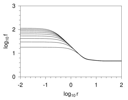
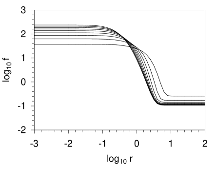
(a)	(b)

Figure 1: The log-log plot of the correlation function $f\equiv r^{5}\langle T^{++}(x)T^{++}(0)\rangle\left({x^{-}\over x^{+}}\right)^{2}\frac{16\pi^{3}}{105}{{K^{3}l}\over\sqrt{-i}}$ vs. $r$ (a) in units where $g=g_{\rm YM}\sqrt{N_{c}l}/2\pi^{3/2}=0.10$ for $K=4$ and $T=1$ to 9; (b) in units where $g=g_{\rm YM}\sqrt{N_{c}l}/2\pi^{3/2}=1$ for $K=5$ and $T=1$ to 9.

The correlator converges from below at small $r$ with increasing $T$, and in the region $-0.5\leq\log r\leq 0.5$ the plot of $r^{5}$ times the correlator falls like $1/r$. In Fig. 2 at resolution $K=5$ we see the same behavior for strong coupling ($g=g_{\rm YM}\sqrt{N_{c}l}/2\pi^{3/2}=10$) but now at smaller $r$ ($\log r\simeq-0.5$) as one would expect.

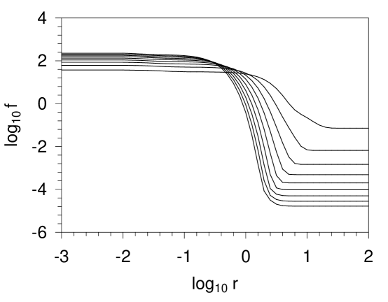
Figure 2: Same as Fig. 1(b), but for $g=g_{\rm YM}\sqrt{N_{c}l}/2\pi^{3/2}=10$.

Again at strong coupling we see that the correlator converges quickly and from below in $T$. All indications are that at small $r$ the correlators are well approximated by SDLCQ, converge rapidly, and show the behavior that one would expect on general physical grounds. This gives us confidence to go on to investigate the behavior at large $r$.

The behavior for large $r$ is governed by the massless states. From earlier work [9, 10] on the spectrum of this theory we know that there are two types of massless states. At $g=0$ the massless states are a reflection of all the states of the dimensionally reduced theory in $1+1$. In 2+1 dimensions these states behave as $g^{2}M^{2}_{1+1}$. We expect therefore that for $g\simeq 0$ there should be no dependence of the correlator on the transverse momentum cutoff $T$ at large $r$. In Fig. 1(a) this behavior is clearly evident.

At all couplings there are exactly massless states which are the BPS states of this theory, which has zero central charge. These states are destroyed by one supercharge, $Q^{-}$, and not the other, $Q^{+}$. From earlier work [9] on the spectrum we saw that the number of BPS states is independent of the transverse resolution and equal to $2K-1$. Since these states are exactly massless at all resolutions, transverse and longitudinal convergence of these states cannot be investigated using the spectrum. These states do have a complicated dependence on the coupling $g$ through their wave function, however. This is a feature so far not encountered in DLCQ [14]. In previous DLCQ calculations one always looked to the convergence of the spectrum as a measure of the convergence of the numerical calculation. Here we see that it is the correlator at large $r$ that provides a window to study the convergence of the wave functions of the BPS states. In Fig. 2 we see that the correlator converges from above at large $r$ as we increase $T$.

We also note that the correlator at large $r$ is significantly smaller than at small $r$, particularly at strong coupling. In our initial study of the BPS states [10] we found that at strong coupling the average number of particles in these BPS states is large. Therefore the two particle components, which are the only components the $T^{++}$ correlator sees, are small.

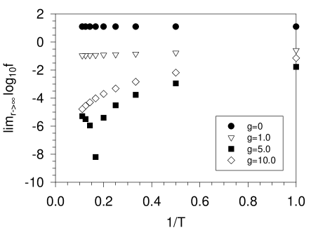
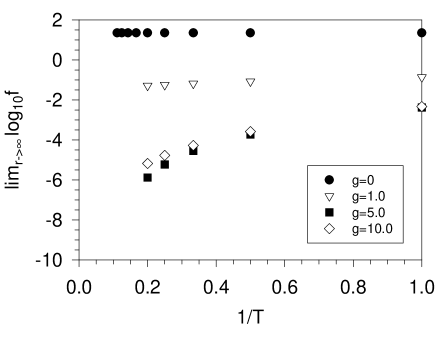
(a)	(b)

Figure 3: The large-$r$ limit of the log of the correlation function $f\equiv r^{5}\langle T^{++}(x)T^{++}(0)\rangle\left({x^{-}\over x^{+}}\right)^{2}\frac{16\pi^{3}}{105}{{K^{3}l}\over\sqrt{-i}}$ vs. $1/T$ for (a) $K=5$ and (b) $K=6$ and for various values of the coupling $g=g_{\rm YM}\sqrt{N_{c}l}/2\pi^{3/2}$.

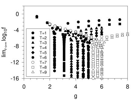
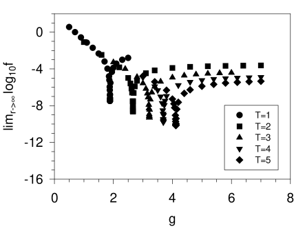
(a)	(b)

Figure 4: The large-$r$ limit of the correlation function $f\equiv r^{5}\langle T^{++}(x)T^{++}(0)\rangle\left({x^{-}\over x^{+}}\right)^{2}\frac{16\pi^{3}}{105}{{K^{3}l}\over\sqrt{-i}}$ vs. $g=g_{\rm YM}\sqrt{N_{c}l}/2\pi^{3/2}$ for (a) $K=5$ (b) $K=6$ and for various values of the transverse resolution $T$.

The coupling dependence of the large-$r$ limit of the correlator is much more interesting than we would have expected based on our previous work on the spectrum. To see this behavior we study the large-$r$ behavior of the correlator at fixed $g$ as a function of the transverse resolution $T$ and at fixed $T$ as a function of the coupling $g$. We see a hint that something unusual is occurring in Fig. 3. For values of the coupling up to about $g=1$ we see the typical rapid convergence in the transverse momentum cutoff; however, at larger coupling the convergence appears to deteriorate, and we see that for $g=5$ the correlator is smaller than at $g=10$. We see this same behavior at both $K=5$ and $K=6$. In Fig. 4 we see that the correlator does not in fact decrease monotonically with $g$ but rather has a singularity at a particular value of the coupling which is a function of $K$ and $T$. Beyond the singularity the correlator again appears to behave well.

If we plot the ‘critical’ couplings, at which the correlator goes to zero, versus $\sqrt{T}$, as in Fig. 5, we see that they lie on a straight line, i.e. this coupling is a linear function of $\sqrt{T}$ in both cases, $K=5$ and 6. Consequently, the ‘critical’ coupling goes to infinity in the transverse continuum limit. It appears as though we have encountered a finite transverse cutoff effect. The most likely conclusion is that our numerical calculation of the BPS wave function is only valid for $g<g_{\rm crit}(T)$. While the large-$r$ correlator does converge above the critical coupling, it is unclear at this time if it has any significance. It might have been expected that one would need larger and larger transverse resolution to probe the strong coupling region, the occurrence of the singular behavior that we see is a surprise, and we have no detailed explanation for it at this time. We see no evidence of a singular behavior at small or intermediate $r$. This indicates, but does not prove, that our calculations of the massive bound states is valid at all $g$.

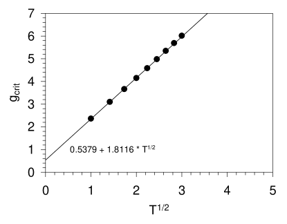
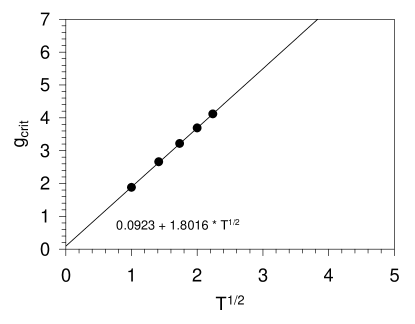
(a)	(b)

Figure 5: Critical coupling $g_{\rm crit}$ versus $\sqrt{T}$ for (a) $K=5$ and (b) $K=6$.

We do not seem to see a region dominated the massive bound states, that is, a region where $r$ is large enough that we see the structure of the bound states but small enough that the correlator is not dominated by the massless states of the theory. Such a region might give us other important information about this theory.

6 Conclusion

In this work we calculate the correlator $\langle 0|T^{++}(x)T^{++}(0)|0\rangle$ in ${\cal N}=1,$ SYM in 2+1 dimension at large $N_{c}$ in the collinear limit. We find that the free-particle correlator behaves like $1/r^{6}$, in agreement with results from conformal field theory. The contribution from an individual bound state is found to behave like $1/r^{5}$, and at small $r$ such contributions conspire to reproduce the conformal field theory result $1/r^{6}$. We do not seem to find an intermediate region in $r$ where the correlator behaves as $1/r^{5}$, reflecting the behavior of the individual massive bound states.

At large $r$ the correlator is dominated by the massless BPS states of the theory. We find that as a function of $g$ the large-$r$ correlator has a critical value of $g$ where it abruptly drops to zero. We have investigated this singular behavior and find that at fixed longitudinal resolution the critical coupling grows linearly with $\sqrt{T}$. We conjecture that this critical coupling signals the breakdown of SDLCQ at sufficiently strong coupling at fixed transverse resolution, $T$. While this might not be surprising in general, it is surprising that the behavior appears in the BPS wave functions and that we see no sign of this behavior in the massive states. We find that above the critical coupling the correlator still converges but significantly slower. It is unclear at this time if we should attach any significance to the correlator in this region.

This calculation emphasizes the importance of BPS wave functions which carry important coupling dependence, even though the mass eigenvalues are independent of the coupling. We will discuss the spectrum, the wavefunctions and associated properties of all the low energy bound states of ${\cal N}=1$ SYM in 2+1 dimensions in a subsequent paper [19].

A number of computational improvements have been implemented in our code to allow us to make these detailed calculations. The code now fully utilizes the three known discrete symmetries of the theory, namely supersymmetry, transverse parity $P$, Eq. (14), and the $Z_{2}$ symmetry $S$, Eq. (15). This reduces the dimension of the Hamiltonian matrix by a factor of 8. Other, more efficient storage techniques allow us to handle on the order of 2,000,000 states in this calculation, which has been performed on a single processor Linux workstation. Our improved storage techniques should allow us to expand this calculation to include higher supersymmetries without a significant expansion of the code or computational power. We remain hopeful that porting to a parallel machine will allow us to tackle problems in full 3+1 dimensions.

References

- [1] F. Antonuccio, O. Lunin, S. Pinsky, and A. Hashimoto, JHEP 07 (1999) 029.
- [2] J.R. Hiller, O. Lunin, S. Pinsky, U. Trittmann, Phys. Lett. B482 (2000) 409, hep-th/0003249.
- [3] J. Maldacena, Adv. Theor. Math. Phys. 2 (1998) 231, hep-th/9711200.
- [4] Y. Matsumura, N. Sakai, and T. Sakai, Phys. Rev. D52 (1995) 2446, hep-th/9504150.
- [5] A. Hashimoto and I.R. Klebanov, Nucl. Phys. B434 (1995) 264, hep-th/9409064.
- [6] F. Antonuccio, O. Lunin, S. Pinsky, Phys. Lett. B429 (1998) 327, hep-th/9803027.
- [7] F. Antonuccio, O. Lunin, and S. Pinsky, Phys. Rev. D58 (1998) 085009, hep-th/9803170.
- [8] O. Lunin and S. Pinsky, in the proceedings of 11th International Light-Cone School and Workshop: New Directions in Quantum Chromodynamics and 12th Nuclear Physics Summer School and Symposium (NuSS 99), Seoul, Korea, 26 May - 26 Jun 1999 (New York, AIP, 1999), p. 140, hep-th/9910222.
- [9] P. Haney, J.R. Hiller, O. Lunin, S. Pinsky, and U. Trittmann, Phys. Rev. D62 (2000) 075002, hep-th/9911243.
- [10] F. Antonuccio, O. Lunin, and S. Pinsky, Phys. Rev. D59 (1999) 085001, hep-th/9811083.
- [11] S.S. Gubser, I.R. Klebanov, and A.M. Polyakov, Phys. Lett. B428 (1998) 105, hep-th/9802109.
- [12] E. Witten, Adv. Theor. Math. Phys. 2 (1998) 253, hep-th/9802150.
- [13] H. Osborn and A.C. Petkou, Ann. Phys. 231 (1994) 311, hep-th/9307010.
- [14] S.J. Brodsky, H.-C. Pauli, and S.S. Pinsky, Phys. Rep. 301 (1998) 299, hep-ph/9705477.
- [15] D. Kutasov, Phys. Rev. D48 (1993) 4980, hep-th/9306013.
- [16] G. Bhanot, K. Demeterfi, and I.R. Klebanov, Phys. Rev. D48 (1993) 4980, hep-th/9307111.
- [17] F. Antonuccio, O. Lunin, H.-C. Pauli, S. Pinsky, and S. Tsujimaru, Phys. Rev. D58 (1998) 105024, hep-th/9806133.
- [18] C. Lanczos, J. Res. Nat. Bur. Stand. 45, 255 (1950); J. Cullum and R.A. Willoughby, Lanczos Algorithms for Large Symmetric Eigenvalue Computations, Vol. I and II, (Birkhauser, Boston, 1985).
- [19] J.R. Hiller, S. Pinsky, and U. Trittmann, in preparation.