SU-ITP 00-37 YITP-00-72 hep-th/0012270
Low-energy propagation modes on string network

We study low-energy propagation modes on string network lattice. Specifically, we consider an infinite two-dimensional regular hexagonal string network and analyze the low frequency propagation modes on it. The fluctuation modes tangent to the two-dimensional plane respect the spatial rotational symmetry on the plane, and are described by Maxwell theory. The gauge symmetry comes from the marginal deformation of changing the sizes of the loops of the lattice. The effective Lorentz symmetry respected at low energy will be violated at high energy.

In type IIB string theory, it is known that there exist configurations in which different kind of strings meet and form junctions [1, 2]. These configurations are stabilized by the conservation of the two-form charges of strings and the force balance conditions at junctions [1, 2]. Connecting many of such junctions, string network can be constructed [3] (Fig.1). Now the system can be a macroscopic object. In [4], the expression for its macroscopic entropy was conjectured and the network system was compared with a black hole. In the present short note, we rather regard it as a space. This might be similar in spirit to the idea of brane world [5, 6] and also to the network appearing in quantum gravity [7, 8, 9, 10, 11]. We shall discuss the low frequency propagation modes on it. Some discussions with similar interests have already appeared in [12, 13].

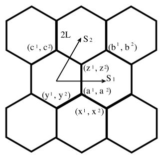
Figure 1: The hexagonal string network lattice. The length of each string is $2L$. The coordinate fluctuations of the vertices from their regular locations are denoted by $(x^{1},x^{2})$, etc. There are two independent discrete translation symmetries $S_{1},S_{2}$.

The potential energy of this network is given by

$$V=\sum_{\langle\alpha\beta\rangle}T_{\alpha\beta}|x_{\alpha}-x_{\beta}|,$$ (1)

where the Greek indices $\alpha,\beta$ are the labels of the vertices of the network and $T_{\alpha\beta}$ denotes the tension of the string connecting the vertex pair $\alpha$ and $\beta$. Here $x_{\alpha}$ denotes the location of the vertex $\alpha$, and the sum is over all the vertex pairs connected by a string.

It is known that a string network with loops can be deformed without changing the potential energy. This marginal deformation is given by changing the size of each loop while the angles between the strings are kept unchanged (Fig.2). This is because the stability condition at the vertices remains valid after the change of the size of the loop due to the constancy of string tension. Especially when the whole configuration is within a two-dimensional plane, the configuration can be shown to be BPS [14, 3]. Thus the remaining supersymmetries guarantee that the marginal modes are exactly the zero-modes of the potential energy.

Figure 2: A marginal deformation of a string network.

This marginal deformation exists for each loop. Hence for the low frequency propagation modes along the network, this marginal deformation may be observed as a local symmetry of the potential energy. We will show that the low frequency modes on the lattice have only physical vibrations transverse to the momentum and the marginal deformation may be regarded as a $U(1)$ gauge symmetry of effective Maxwell theory.

The details of the propagation modes will depend on the details of the network configuration, which are determined by the charge assignment of the strings in the network and the string coupling constant. However some rough essential properties will not. Thus for simplicity, in this short note, we assume that the tensions of the strings in the network are all equal, $T_{\alpha\beta}=T$, and the strings form an infinite regular two-dimensional hexagonal lattice. This setting can be easily realized by choosing appropriate charges of the strings and an appropriate string coupling constant.

Another simplification in this note is that we consider only small fluctuations of the lattice configuration. An interesting aspect will obviously appear when we consider large fluctuations. Especially we may change the topology of the lattice by combining the marginal deformations as in Fig.3. This should be regarded as a change of the effective geometry generated by the string network rather than the changes of fields on it. In one sense, this would be a very interesting property of this network system, but presently we do not have any ideas to incorporate such topological changes in the following calculation. In the following discussions we will take into account the fluctuations from the regular hexagonal lattice only up to second order.

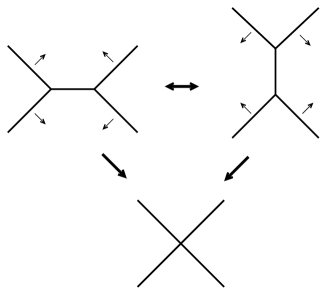
Figure 3: The topology of a string network can be changed by successive applications of the marginal deformation.

There are only two kinds of vertices in the hexagonal lattice, namely like one at $(a^{1},a^{2})$ and like one at $(z^{1},z^{2})$ in Fig.1, for example. Let us look at the minimal part including these two vertices and their neighbors as in Fig.1. For the meanwhile, we consider the fluctuations of the lattice tangent to the two-dimensional plane. The parameterizations of the vertex locations are given in Fig.1. The $(a^{1},a^{2})$, etc., denote the deviations of the junction points from the regular locations of the vertices of the hexagonal lattice. We assume the length of the edges of the hexagonal lattice is $2L$. Then, up to second order, we easily obtain the change of the potential energy as

$$\delta V_{(a^{1},a^{2})} = \frac{T}{8L}\Big{(}3(a^{1})^{2}+3(a^{2})^{2}-a^{1}(x^{1}+\sqrt{3}x^{2}+y^{1}-\sqrt{3}y^{2}+4z^{1})$$ (3)

$$\hskip 113.81102pt-a^{2}(\sqrt{3}x^{1}+3x^{2}-\sqrt{3}y^{1}+3y^{2})\Big{)},$$

where we have evaluated only the part which contains the parameter $(a^{1},a^{2})$. In this evaluation, we assumed that the strings are straight lines between the junctions. This approximation is enough for the long wave length analysis of this paper, but will become bad when the wave length becomes comparable with the length of a string. In such a high energy case, we need to analyze the propagation of a wave on each string as was studied in [12, 13].

As for $(z^{1},z^{2})$, the potential change can be obtained just by appropriate replacements of the parameters in (3):

$$\delta V_{(z^{1},z^{2})} = \frac{T}{8L}\Big{(}3(z^{1})^{2}+3(z^{2})^{2}+z^{1}(-b^{1}+\sqrt{3}b^{2}-c^{1}-\sqrt{3}c^{2}-4a^{1})$$ (5)

$$\hskip 113.81102pt+z^{2}(\sqrt{3}b^{1}-3b^{2}-\sqrt{3}c^{1}-3c^{2})\Big{)}.$$

The total change of the potential energy is obtained by summing over all the contributions of like (3) and (5) in the lattice.

Now we want to diagonalize the total change of the potential energy, $\delta V=\sum_{\alpha}\delta V_{\alpha}$. This is easy if we use the discrete symmetries of the hexagonal lattice. The hexagonal lattice has the discrete translation symmetries $S_{1},S_{2}$, as is shown in Fig.1. Hence $\delta V$ can be diagonalized in the subspace of the eigen space of the discrete translations. Let us take the phase shift associated to each discrete translation as $S_{i}=\exp(i\theta_{i})$. Then, in this particular subspace, the parameters in Fig.1 are related by

$$y^{i} = S_{2}^{-1}z^{i}=e^{-i\theta_{2}}z^{i},$$ (6)

$$x^{i} = S_{1}y^{i}=e^{i\theta_{1}-i\theta_{2}}z^{i},$$ (7)

$$b^{i} = S_{2}a^{i}=e^{i\theta_{2}}a^{i},$$ (8)

$$c^{i} = S_{1}^{-1}b^{i}=e^{-i\theta_{1}+i\theta_{2}}a^{i}.$$ (9)

Then substituting (6) into the eigen value equations

$$\frac{\partial\delta V_{(a^{1},a^{2})}}{\partial a^{1}} = 2va^{1},$$ (10)

$$\frac{\partial\delta V_{(a^{1},a^{2})}}{\partial a^{2}} = 2va^{2},$$ (11)

$$\frac{\partial\delta V_{(z^{1},z^{2})}}{\partial z^{1}} = 2vz^{1},$$ (12)

$$\frac{\partial\delta V_{(z^{1},z^{2})}}{\partial z^{2}} = 2vz^{2},$$ (13)

we obtain linear equations for the variables $a^{1,2}$ and $z^{1,2}$. From the requirement for the equations (10) to have non-trivial solutions, the eigenvalues are given by

$$v=0,\ \frac{3T}{4L},\ \frac{T}{8L}\left(3\pm\sqrt{3+2\cos{\theta_{1}}+2\cos{\theta_{2}}+2\cos{(\theta_{1}-\theta_{2})}}\right).$$ (14)

The vanishing eigen value should come from the zero modes of changing the loop sizes. From (14), we see that there is another low energy mode at low frequency parameter region $\theta_{1},\theta_{2}\sim 0$. In the second order of $\theta_{1},\theta_{2}$, the eigen value is expressed as

$$v_{low}=\frac{T}{24L}(\theta_{1}^{2}-\theta_{1}\theta_{2}+\theta_{2}^{2}).$$ (15)

Since the $S_{1}$ and $S_{2}$ are the translations by the vectors $(2\sqrt{3}L,0)$ and $(\sqrt{3}L,3L)$ and the phase shifts associated to them are $\theta_{1}$ and $\theta_{2}$, respectively, the relation between momentum $(p_{1},p_{2})$ and the parameters $\theta_{1},\theta_{2}$ should be given by

$$\theta_{1} = 2\sqrt{3}Lp_{1},$$ (16)

$$\theta_{2} = \sqrt{3}Lp_{1}+3Lp_{2}.$$ (17)

Substituting this relation to (15), we obtain

$$v_{low}=\frac{3TL}{8}(p_{1}^{2}+p_{2}^{2})$$ (18)

as the expression of the eigen value of the potential energy in the second order of momentum. This shows that the spatial rotational symmetry is recovered, and that the mode is massless.

To investigate further the properties of these modes, let us discuss the eigenvector of (10). In the lowest order of $\theta_{1},\theta_{2}$, we obtain the eigen vector for $v_{low}$ as

$$\left(\begin{array}[]{c}a^{1}\\ a^{2}\\ z^{1}\\ z^{2}\end{array}\right)_{v=v_{low}}=\left(\begin{array}[]{c}\frac{\theta_{1}-2\theta_{2}}{\sqrt{3}}\\ \theta_{1}\\ \frac{\theta_{1}-2\theta_{2}}{\sqrt{3}}\\ \theta_{1}\end{array}\right)\propto\left(\begin{array}[]{c}-p_{2}\\ p_{1}\\ -p_{2}\\ p_{1},\end{array}\right).$$ (19)

This shows that this fluctuation is orthogonal to momentum. This recalls us the fact that only the transverse degrees of freedom is the physical ones in gauge theory. In fact, the eigen vector related to the vanishing eigen value is given by

$$\left(\begin{array}[]{c}a^{1}\\ a^{2}\\ z^{1}\\ z^{2}\end{array}\right)_{v=0}=\left(\begin{array}[]{c}\theta_{1}\\ \frac{-\theta_{1}+2\theta_{2}}{\sqrt{3}}\\ \theta_{1}\\ \frac{-\theta_{1}+2\theta_{2}}{\sqrt{3}}\end{array}\right)\propto\left(\begin{array}[]{c}p_{1}\\ p_{2}\\ p_{1}\\ p_{2}\end{array}\right).$$ (20)

Hence the fluctuation related to the zero modes is in fact in the longitudinal direction and is consistent with the interpretation that it is the gauge degrees of freedom of Maxwell theory.

Now let us discuss the kinetic energy. In this low frequency approximation, it is enough to estimate the kinetic energy just by assuming that a string portion moves with the nearest vertex point. The total string length associated to each vertex is $3L$. Taking into account the fact that only the motions transverse to the strings contribute to the kinetic energy, the kinetic term becomes

$$K=\frac{3TL}{4}\sum_{\alpha}\left[\left(\frac{dx_{\alpha}^{1}}{dt}\right)^{2}+\left(\frac{dx_{\alpha}^{2}}{dt}\right)^{2}\right],$$ (21)

where $\alpha$ denotes the vertex points and its location deviation is denoted as $(x_{\alpha}^{1},x_{\alpha}^{2})$.

It is now easy to write down the effective action. Let us denote $A^{i}(t,\sigma^{1},\sigma^{2})\ (i=1,2)$ on an effective two-dimensional plane $(\sigma^{1},\sigma^{2})$ as the collective coordinate of the location deviation of the vertices. From the above discussion on the polarization of the zero modes, there is a gauge symmetry in the same form as that of Maxwell theory:

$$\delta A^{i}=L\frac{\partial\Lambda(\sigma)}{\partial\sigma^{i}}.$$ (22)

The potential energy of the field $A^{i}$ should respect the two-dimensional spatial rotational symmetry and the gauge symmetry (22). Hence its possible form quadratic in $A_{i}$ is given by $(\epsilon^{ij}\partial A^{i}/\partial\sigma^{j})^{2}$. The numerical factor is determined from (18). Thus, also from (21), we obtain the effective Lagrangian

$$L_{eff} = \int\frac{d^{2}\sigma}{3\sqrt{3}L^{2}}\left[\frac{3TL}{4}\left(\frac{\partial A^{i}}{\partial t}\right)^{2}-\frac{3TL}{8}\left(\epsilon^{ij}\frac{\partial A^{i}}{\partial\sigma^{j}}\right)^{2}\right]$$ (23)

$$= \frac{T}{2\sqrt{3}L}\int d^{2}\sigma\left[\frac{1}{2}\left(\frac{\partial A^{i}}{\partial t}\right)^{2}-\frac{1}{4}\left(\epsilon^{ij}\frac{\partial A^{i}}{\partial\sigma^{j}}\right)^{2}\right].$$ (24)

The factor $3\sqrt{3}L^{2}$ in the denominator is the area associated to each vertex, and we have substituted $\sum_{\alpha}$ with $\int d^{2}\sigma/3\sqrt{3}L^{2}$. This effective Lagrangian (23) is just the Lagrangian of Maxwell theory with the gauge $A^{0}=0$ and with the effective velocity of “photon”, $c_{eff}=1/\sqrt{2}$.

When we take the $A^{0}=0$ gauge of Maxwell theory, we obtain the Gauss law constraint

$$\partial_{0}\partial_{i}A^{i}=0.$$ (25)

On the other hand, what we obtain from the equations of motion of (23) is only a weaker equation

$${\partial_{0}}^{2}\partial_{i}A^{i}=0.$$ (26)

In the lattice language, $\partial_{i}A^{i}$ describes the fluctuation of the local density of the vertices. This local density can be changed by marginal deformations, and hence is not a dynamical quantity in the low energy physics. The Gauss law constraint (25) does not allow $\partial_{i}A^{i}$ to be dynamical and incorporates correctly this fact. Thus we insist that the low energy physics is described by Maxwell theory but not simply by the Lagrangian (23).

Now let us consider the fluctuations in the directions transverse to the two-dimensional lattice plane. Let us use $a^{m},b^{m},c^{m},x^{m},y^{m},z^{m}\ (m=3,\cdots,9)$ as the transverse fluctuations of the parameterized vertices in Fig.1. Then, up to second order, the changes of the parts of the potential energy containing the parameters $a^{m},z^{m}$ are given by

$$\delta V_{a^{m}} = \frac{T}{4L}(3(a^{m})^{2}-2a^{m}(x^{m}+y^{m}+z^{m})),$$ (27)

$$\delta V_{z^{m}} = \frac{T}{4L}(3(z^{m})^{2}-2z^{m}(a^{m}+b^{m}+c^{m})),$$ (28)

respectively. Performing similar analysis as above, the eigenvalues of the potential is obtained as

$$v^{trans}=\frac{T}{4L}\left(3\pm\sqrt{3+2\cos{\theta_{1}}+2\cos{\theta_{2}}+2\cos{(\theta_{1}-\theta_{2})}}\right).$$ (29)

This is just twice of two of what appeared in (14). Thus as for the transverse fluctuations, the effective Lagrangian becomes

$$L_{eff}^{trans}=\frac{T}{\sqrt{3}L}\int d^{2}\sigma\ \left[\frac{1}{2}\left(\frac{\partial\phi^{m}}{\partial t}\right)^{2}-\frac{1}{4}\left(\frac{\partial\phi^{m}}{\partial\sigma^{j}}\right)^{2}\right].$$ (30)

The velocity of this propagation is given by $c^{trans}_{eff}=1/\sqrt{2}$, which is equivalent to the above one of Maxwell theory.

Since the two kinds of massless fields propagate similarly, one low energy effective geometry is associated to the string lattice. There is a Lorentz symmetry which keeps the geometry and the field propagations invariant. However, the Lorentz symmetry of the effective theory is different from the proper Lorentz symmetry of IIB string theory. Thus in the high energy region, the effective Lorentz symmetry will be violated. This aspect will appear in a way as follows. Although the zero modes of changing the loop sizes are the gauge symmetry of the effective action, this is not the symmetry of the full theory. The reason why we could ignore it in our discussions so far is that, since this zero mode does not change the energy density coming from string tension in the macroscopic scale, it does not couple with the collective modes in the approximation of low frequency. On the other hand, at high frequency, the gauge mode will become relevant, and the people living on the two-dimensional plane will detect it as the violation of their Lorentz symmetry. A rough estimation of the coupling of the gauge mode $\Lambda(\sigma)$ with the collective mode goes as follows. Let us consider the kinetic energy from a string connecting the vertices at $x_{\alpha}$ and $x_{\beta}$. In the next order of low frequency approximation, the following contribution of the kinetic energy will be relevant:

$$\delta K_{\alpha\beta}\sim LT\frac{dx_{\alpha}}{dt}\frac{dx_{\beta}}{dt}.$$ (31)

Thus, using the variables of the effective theory, this is approximately

$$\delta K\sim\sum_{\langle\alpha\beta\rangle}\delta K_{\alpha\beta} \sim LT\int\frac{d^{2}\sigma}{L^{2}}\frac{\partial A(\sigma)}{\partial t}\frac{\partial A(\sigma+L+\Lambda)}{\partial t}$$ (32)

$$\sim T\int d^{2}\sigma\frac{\partial^{2}A^{i}}{\partial t\partial\sigma^{j}}\frac{\partial^{2}A_{i}}{\partial t\partial\sigma_{j}}\Lambda,$$ (33)

where, in the second line, a term which does not couple to $\Lambda$ is ignored. From the first to the second line, we took the second term in the expansion in terms of $L+\Lambda$, on the assumption that the result would respect the spatial rotational symmetry. The coupling (32) is certainly a non-renormalizable high dimensional term, and is irrelevant at low energy but will become relevant at high energy.

Some comments are in order.

It is known that a two-dimensional string network configuration respects a quarter of the supersymmetries of IIB string theory [14, 3]. Thus it is expected that there exist fermionic low energy modes which form supermultiplets with the bosonic modes of the effective field theory. It would be an interesting question how the multiplet structures are given in this non-relativistic effective field theory.

It is also possible that a stable string network forms a higher dimensional effective manifold. Such a configuration would be made stable, and the modes of changing the sizes of loops would be zero-modes in the lowest approximation. However, in this case, all the supersymmetries are violated, and the system will have effects from the interactions among strings and also from some quantum corrections. These effects may be considerably large especially on the marginal modes, and hence the low-energy theory may be very different from the two-dimensional case studied in this paper.

In this short note, we considered only small fluctuations of the vertices from their regular locations just for technical simplicity. Since the marginal modes are the exact flat directions of the potential energy in the two-dimensional case, there does not seem to exist any reasons enough to support this perturbative truncation. Large fluctuations deform not only the lattice geometry but also the connectivity of the lattice. This fact suggests that the effective theory should contain a quantum-gravity-like theory but not a field theory alone as was discussed in this paper. Thus the results presented in this paper would make sense, only if the effective theory is combined with a certain gravity-like theory, or only if there exists a certain mechanism to keep a string network near around a certain reference configuration by suppressing large zero-mode fluctuations.

Acknowledgments
The author would like to thank A. Hashimoto, S. Hirano, L. Susskind and N. Toumbas for stimulating discussions and comments, and K. Hashimoto for the careful reading of the manuscript and helpful comments. The author is supported in part by the Fellowship Program for Japanese Scholars and Researchers to study abroad, in part by Grant-in-Aid for Scientific Research (#12740150), and in part by Priority Area: “Supersymmetry and Unified Theory of Elementary Particles” (#707), from Ministry of Education, Science, Sports and Culture, Japan.

References

- [1] J. H. Schwarz, “Lectures on superstring and M theory dualities,” Nucl. Phys. Proc. Suppl. 55B, 1 (1997) [hep-th/9607201].
- [2] O. Aharony, J. Sonnenschein and S. Yankielowicz, “Interactions of strings and D-branes from M theory,” Nucl. Phys. B474, 309 (1996) [hep-th/9603009].
- [3] A. Sen, “String network,” JHEP9803, 005 (1998) [hep-th/9711130].
- [4] B. Kol, “Thermal monopoles,” JHEP0007, 026 (2000) [hep-th/9812021].
- [5] N. Arkani-Hamed, S. Dimopoulos and G. Dvali, “The hierarchy problem and new dimensions at a millimeter,” Phys. Lett. B429, 263 (1998) [hep-ph/9803315].
- [6] L. Randall and R. Sundrum, “Out of this world supersymmetry breaking,” Nucl. Phys. B557, 79 (1999) [hep-th/9810155].
- [7] T. Regge, “General Relativity Without Coordinates,” Nuovo Cim. 19, 558 (1961).
- [8] R. Penrose, in Quantum theory and beyond ed. T. Bastin, Cambridge U Press 1971.
- [9] C. Rovelli and L. Smolin, “Spin networks and quantum gravity,” Phys. Rev. D 52, 5743 (1995) [gr-qc/9505006].
- [10] H. Ooguri and N. Sasakura, “Discrete and continuum approaches to three-dimensional quantum gravity,” Mod. Phys. Lett. A6, 3591 (1991) [hep-th/9108006].
- [11] J. Ambjorn, B. Durhuus and T. Jonsson, “Quantum geometry. A statistical field theory approach,” Cambridge, UK: Univ. Pr. (1997) 363 p.
- [12] S. Rey and J. Yee, “BPS dynamics of triple (p,q) string junction,” Nucl. Phys. B526, 229 (1998) [hep-th/9711202].
- [13] C. G. Callan and L. Thorlacius, “Worldsheet dynamics of string junctions,” Nucl. Phys. B534, 121 (1998) [hep-th/9803097].
- [14] K. Dasgupta and S. Mukhi, “BPS nature of 3-string junctions,” Phys. Lett. B423, 261 (1998) [hep-th/9711094].