Self-dual Chern-Simons solitons in noncommutative space

Abstract

We construct exact soliton solutions to the Chern-Simons-Higgs system in noncommutative space, for non-relativistic and relativistic models. In both cases we find regular vortex-like solutions to the BPS equations which approach the ordinary selfdual non-topological and topological solitons when he noncommutative parameter $\theta$ goes to zero.

1 Introduction

After the connection between string theory and noncommutative field theories was unraveled [1]-[3], the study of solitons and instantons in noncommutative spacetimes has attracted much attention [4]-[18]. Chern-Simons (CS) theories in commutative space have played a central role for the understanding of relevant phenomena in planar physics [19],[20] and some of their properties started to be explored recently in the noncommutative case [21]-[27].

In ordinary $2+1$ dimensional space, models of relativistic and non-relativistic matter minimally coupled to gauge fields whose dynamics is governed by a CS term have self-dual vortex-like solutions[28]-[30]. It is then interesting to determine if this kind of solutions are also present in the non-commutative extension of these models. In this work we shall study the existence and properties of vortex-like solitons for Chern-Simons matter systems in noncommutative $2+1$ dimensional space. Our approach follows closely that developed in [18] for constructing exact noncommutative vortex solutions in the Maxwell-Higgs system except that now the dynamics of the gauge field is governed by a CS Lagrangian. Also, we consider the nonrelativistic case introduced in [28] in view of its relevance for studying Bohm-Aharonov effect and other interesting phenomena in planar physics.

After introducing the noncommutative models in section 2, we derive BPS equations and construct explicit solutions in the nonrelativistic case in section 3. We find a family of non-topological BPS solitons parametrized by a constant $f_{0}$. The corresponding magnetic flux $\Phi$ is in general non quantized but becomes an integer in the $\theta\to 0$ limit. In section 4 we consider the relativistic case, and construct BPS topological solitons with quantized magnetic flux which coincide with the regular ordinary vortex solutions when $\theta\to 0$. Finally, we present our conclusions in section 5.

2 The model

We consider 3-dimensional space-time with coordinates $X^{\mu}$ ($i=0,1,2$) obeying the following noncommutative relations

$$[X^{\mu},X^{\nu}]=i\theta^{\mu\nu}$$ (1)

The real antisymmetric matrix $\theta^{\mu\nu}$, can be brought into its canonical (Darboux) form by an appropriate orthogonal rotation

$$[X^{1},X^{2}]=i\theta\,,\;\;\;\;\;[X^{1},X^{0}]=[X^{2},X^{0}]=0$$ (2)

One way to describe field theories in noncommutative space is by introducing a Moyal product $*$ between ordinary functions. To this end, one can establish a one to one correspondence between operators $\hat{f}$ and ordinary functions $f$ through a Weyl ordering

$$\hat{f}(X^{1},X^{2})=\frac{1}{2\pi}\int d^{2}k\tilde{f}(k_{1},k_{2})\exp\left(i(k_{1}X^{1}+k_{2}X^{2})\right)$$ (3)

Then, the product of two Weyl ordered operators $\hat{f}\hat{g}$ corresponds to a function $f*g(x)$ defined as

$$f*g(x)=\left.\exp\left(\frac{i\theta}{2}(\partial_{x_{1}}\partial_{y_{2}}-\partial_{x_{2}}\partial_{y_{1}})\right)f(x_{1},x_{2})g(y_{1},y_{2})\right|_{x_{1}=x_{2},y_{1}=y_{2}}$$ (4)

Given a $U(1)$ gauge field $A_{\mu}(x)$, the field strength $F_{\mu\nu}$ is defined as

$$F_{\mu\nu}=\partial_{\mu}A_{\nu}-\partial_{\nu}A_{\mu}-i(A_{\mu}*A_{\nu}-A_{\nu}*A_{\mu})$$ (5)

We shall couple the gauge field to a complex scalar field $\phi$ with covariant derivative

$$D_{\mu}\phi=\partial_{\mu}\phi-iA_{\mu}*\phi$$ (6)

An alternative approach to noncommutative field theories which has shown to be very useful in finding soliton solutions [6] is to directly work with operators in the phase space $(X^{1},X^{2})$, with commutator (2). In this case the $*$ product is just the product of operators and integration over the $(X^{1},X^{2})$ plane is a trace,

$$\int dx^{1}dx^{2}f(x^{1},x^{2})=2\pi\theta{\rm Tr}\hat{f}(X^{1},X^{2})$$ (7)

In this framework, it is convenient to introduce complex variables $z$ and $\bar{z}$

$$z=\frac{1}{\sqrt{2}}(x^{1}+ix^{2})\,,\;\;\;\;\;\;\bar{z}=\frac{1}{\sqrt{2}}(x^{1}-ix^{2})$$ (8)

and annihilation and creation operators $\hat{a}$ and $\hat{a}^{\dagger}$ in the form

$$\hat{a}=\frac{1}{\sqrt{2\theta}}(X^{1}+iX^{2})\,,\;\;\;\;\;\;\hat{a}^{\dagger}=\frac{1}{\sqrt{2\theta}}(X^{1}-iX^{2})$$ (9)

so that (2) becomes

$$[\hat{a},\hat{a}^{\dagger}]=1$$ (10)

In this way, through the action of $a^{\dagger}$ on the vacuum state $|0\rangle$, eigenstates of the number operator

$$\hat{N}=a^{\dagger}a$$ (11)

are generated. With this conventions, derivatives in the Fock space are given by

$$\partial_{z}=-\frac{1}{\sqrt{\theta}}[\hat{a}^{\dagger},~{}]\,,\;\;\;\;\;\;\partial_{\bar{z}}=\frac{1}{\sqrt{\theta}}[\hat{a},~{}]$$ (12)

After introducing

$$\hat{A}_{z}=\frac{1}{\sqrt{2}}(\hat{A}_{1}-i\hat{A}_{2})\,,\;\;\;\;\hat{A}_{\bar{z}}=\frac{1}{\sqrt{2}}(\hat{A}_{1}+i\hat{A}_{2})$$ (13)

the field strength and covariant derivatives take the form

$$\hat{F}_{z\bar{z}} = \partial_{z}\hat{A}_{\bar{z}}-\partial_{\bar{z}}\hat{A}_{z}-i[\hat{A}_{z},\hat{A}_{\bar{z}}]$$ (14)

$$= -\frac{1}{\sqrt{\theta}}\left([\hat{a}^{\dagger},\hat{A}_{z}]+[\hat{a},A_{\bar{z}}]+i\sqrt{\theta}[\hat{A}_{z},\hat{A}_{\bar{z}}]\right)\equiv i\hat{B}$$

$$D_{\bar{z}}\hat{\phi} = \partial_{\bar{z}}\hat{\phi}-iA_{\bar{z}}\hat{\phi}=\frac{1}{\sqrt{\theta}}[\hat{a},\hat{\phi}]-i\hat{A}_{\bar{z}}\hat{\phi}$$

$$D_{z}\,\hat{\!\bar{\phi}} = \partial_{z}\,\hat{\!\bar{\phi}}+i\hat{A}_{z}\,\hat{\!\bar{\phi}}=-\frac{1}{\sqrt{\theta}}[\hat{a}^{\dagger},\,\hat{\!\bar{\phi}}]+i\hat{A}_{z}\,\hat{\!\bar{\phi}}$$ (15)

with $\hat{B}$ the magnetic field.

We will be interested in the noncommutative extension of the nonrelativistic and relativistic Chern-Simons-matter systems introduced, in ordinary space, in refs.[28]-[30]. The gauge field dynamics for these models is governed by the Chern-Simons Lagrangian $L_{CS}[A]$ defined as

$$L_{CS}[A]=\kappa\;\varepsilon_{\mu\nu\alpha}\left(A_{\mu}*\partial_{\nu}A_{\alpha}-\frac{2i}{3}A_{\mu}*A_{\nu}*A_{\alpha})\right)$$ (16)

The Lagrangian for the noncommutative extension of the non-relativistic case will be taken as

$$L=L_{CS}[A]+i\bar{\phi}*D_{0}\phi+\frac{1}{2}\overline{D_{i}\phi}*D_{i}\phi-\frac{1}{4}\lambda\phi*\bar{\phi}*\phi*\bar{\phi}$$ (17)

while for the relativistic case,

$$L=L_{CS}[A]+\overline{D_{\mu}\phi}*D^{\mu}\phi-V[\phi*\bar{\phi}]$$ (18)

with $V$ the sixth order potential

$$V[\phi*\bar{\phi}]=\frac{1}{\kappa^{2}}\phi*\bar{\phi}*\left(\phi*\bar{\phi}-v^{2}\right)^{2}$$ (19)

taken at the selfdual point, where Bogomol’nyi equations can be found.

3 BPS equations for the non-relativistic case

The Hamiltonian associated with Lagrangian (17) is simply given by

$$H=\int d^{2}x\left(\frac{1}{2}\overline{D_{i}\phi}*D_{i}\phi+\frac{1}{4}\lambda\phi*\bar{\phi}*\phi*\bar{\phi}\right)$$ (20)

It can be written in the form

$$H=\int d^{2}x\left(-\frac{1}{2}\bar{\phi}(D_{1}+i\alpha D_{2})(D_{1}-i\alpha D_{2})\phi+\phi*\bar{\phi}*\left(-\frac{\alpha}{2}F_{12}+\frac{1}{4}\lambda\phi*\bar{\phi}\right)\right)$$ (21)

where $\alpha=\pm 1$. We shall call $\alpha=-1$ the selfdual case and $\alpha=+1$ the anti selfdual one.

Using the Gauss law deriving from Lagrangian (17),

$$\kappa\varepsilon_{ij}F_{ij}+\phi*\bar{\phi}=0$$ (22)

the Hamiltonian takes the form

$$H=\int d^{2}x\left(-\frac{1}{2}\bar{\phi}(D_{1}+i\alpha D_{2})(D_{1}-i\alpha D_{2})\phi-\frac{1}{2}(\alpha+\lambda\kappa)\phi*\bar{\phi}*F_{12}\right)$$ (23)

Then, if the following relation among the two free parameters in the theory holds

$$\lambda\kappa=-\alpha$$ (24)

the lower bound for the Hamiltonian is attained when the following Bogomol’nyi equations are satisfied

$$\left(D_{1}-i\alpha D_{2}\right)\phi=0$$

$$B=-\frac{1}{2\kappa}\phi*\bar{\phi}$$ (25)

Let us first consider the selfdual ($\alpha=-1$) case. In operator language, equations (25) can then be written as

$$D_{\bar{z}}\hat{\phi}=0$$

$$B=-\frac{1}{2\kappa}\hat{\phi}\,\hat{\!\bar{\phi}}$$ (26)

In order to search for vortex solutions to these equations, we propose the ansatz

$$\hat{\phi} = \sqrt{\frac{2|\kappa|}{\theta}}\;\sum_{n=0}^{\infty}f_{n}|n\rangle\langle n+M-1|$$ (27)

$$\hat{A}_{z} = \frac{i}{\sqrt{\theta}}\sum_{n=0}^{\infty}d_{n}|n+1\rangle\langle n|$$ (28)

where $f_{n}$ and $d_{n}$ are arbitrary real coefficients and $\{|n\rangle\}$ is the basis provided by the number operator $\hat{N}$. The ansatz (27) leads, in the $\theta\to 0$ limit, to $\phi\sim\rho(r)z^{M-1}$ which corresponds, in ordinary space, to the usual cylindrically symmetric ansatz with a Higgs field phase $(M-1)\varphi$ [28].

Inserting ansatz (27)-(28) into eq.(26) one obtains the following recurrence relations

$$2\sqrt{p}\,d_{p-1}-d^{2}_{p-1}-2\sqrt{p+1}\,d_{p}+d_{p}^{2}=-\frac{|\kappa|}{\kappa}f_{p}^{2}$$

$$d_{p}=\sqrt{p+1}-\sqrt{p+M}\frac{f_{p}}{f_{p+1}}$$ (29)

which can be combined into the following recurrence relation for the $f_{n}^{\prime}s$ coefficients

$$f_{1}^{2} = \frac{Mf_{0}^{2}}{1-\frac{|\kappa|}{\kappa}f_{0}^{2}}$$

$$f_{p+1}^{2} = \frac{(p+M)f_{p}^{2}}{1-\frac{|\kappa|}{\kappa}f_{p}^{2}+(p+M-1)f_{p-1}^{2}/f_{p}^{2}}\,,\;\;\;\;p\geq 1$$ (30)

If, instead, we choose the anti selfdual case ($\alpha=1$), the equations to solve read

$$D_{z}\hat{\phi}=0$$

$$B=-\frac{1}{2\kappa}\hat{\phi}\,\hat{\!\bar{\phi}}$$ (31)

In this case, the appropriate ansatz is

$$\hat{\phi} = \sqrt{\frac{2|\kappa|}{\theta}}\sum_{n=0}^{\infty}f_{n}|n+M-1\rangle\langle n|$$

$$\hat{A}_{z} = \frac{i}{\sqrt{\theta}}\sum_{n=0}^{\infty}d_{n}|n+1\rangle\langle n|$$ (32)

and the recurrence relations become

$$2\sqrt{p}\,d_{p-1}-d^{2}_{p-1}-2\sqrt{p+1}\,d_{p}+d_{p}^{2}=-\frac{|\kappa|}{\kappa}f_{p-1}^{2}$$

$$d_{p+1}=\sqrt{p+M}-\sqrt{p+1}\frac{f_{p+1}}{f_{p}}$$ (33)

combining to

$$f_{1}^{2} = \left(M-\frac{|\kappa|}{\kappa}f_{0}^{2}\right)f_{0}^{2}$$

$$f_{p+1}^{2} = \frac{1}{p+1}f_{p}^{2}\left(-\frac{|\kappa|}{\kappa}f_{p}^{2}+1+p\frac{f_{p}^{2}}{f_{p-1}^{2}}\right)\,,\;\;\;\;p\geq 1$$ (34)

The flux of the solutions is given by

$$\frac{\Phi}{2\pi}=\theta{\rm Tr}B=-\frac{|\kappa|}{\kappa}\sum_{p}f^{2}_{p}$$ (35)

Finite flux configurations correspond to solutions such that

$$\lim_{p\to\infty}f_{p}=0$$ (36)

The analysis of the asymptotic behavior of the recurrence relation (29) shows that, for large $p$,

$$f^{2}_{p}\rightarrow\frac{1}{p^{\beta}}\;\;\;\;\;$$ (37)

with $\beta$ a real positive parameter to be determined. The flux can also be obtained directly from the expression of $B$ as

$$\frac{\Phi}{2\pi}=\lim_{p\to\infty}\left(d_{p}^{2}-2d_{p}\sqrt{p+1}\right)$$ (38)

Using eqs. (29)-(33) one gets,

$$\frac{\Phi}{2\pi}=M-1+\beta \kappa<0$$ (39)

$$\frac{\Phi}{2\pi}=-M+1-\beta \kappa>0$$ (40)

The numerical study of the recurrence relations reveals that eq.(29) has solutions only for $\kappa<0$ while eq.(33) has solutions only for $\kappa>0$. Thus, as in the commutative case, solutions exist only for $\lambda<0$, that is, only for an “attractive” interaction. Given an initial arbitrary value $f^{2}_{0}$ for the recurrence relation, all coefficients can be determined in such a way that they satisfy (37). Since $\theta$ does not enter explicitly in the recurrence relations, one can construct a whole family of solutions parametrized by $\theta$ (which appears as a factor, see eqs.(28) or (32)).

We have explored numerically the whole $f^{2}_{0}\geq 0$ range finding, for the selfdual case, that there exists, for every value of $f_{0}$, a consistent solution. In contrast, in the anti-selfdual case, the solution ceases to exist for $f_{0}^{2}>M$. This is reminiscent of what happens for non-commutative Nielsen-Olesen anti-selfdual vortices [17].

We have find that $\beta$ is a monotonically increasing function of $f_{0}^{2}$ such that

$$\lim_{f_{0}\to 0}\beta=M+1$$ (41)

Now, according to eqs.(39)-(40) the magnetic flux of our exact solution is in general not quantized in non-commutative space.

We show in figure 1 and 2 the magnetic field $B$ as a function of $r$, for the selfdual and anti-selfdual solutions respectively, computed from eqs.(26),(31). We plot different values of $f_{0}^{2}$ for a given $\theta$. One sees that the $B$ is reminiscent of the magnetic field corresponding to the ordinary (commutative) case, except that in the latter case $B(0)=0$ while in the present noncommutative case $B(0)=B_{0}$, with $B_{0}$ positive (negative) for the selfdual (anti-selfdual) case.

Let us relate at this point this result with that corresponding to ordinary space. As originally shown in [28] Bogomol’nyi equations for the non-relativistic system can be exactly solved since the problem can be reduced to finding solutions to the Liouville equation. Then, the most general axially symmetric regular solution gives, for the selfdual case,

$$\phi^{comm}=\frac{2\sqrt{2|\kappa|}}{r}M\left(\left(\frac{r_{0}}{r}\right)^{M}+\left(\frac{r}{r_{0}}\right)^{M}\right)^{-1}\!\!\exp\left(i(M-1)\,\varphi\right)\;,\;\;\;\;M=1,2,\ldots$$ (42)

where $r_{0}$ is an integration constant. The other free parameter is $M$ which is quantized on regularity grounds. Accordingly, the magnetic flux associated to this solution is quantized,

$$\Phi^{comm}=2\pi(2M)$$ (43)

Note that the flux of our selfdual noncommutative solutions coincides, in the ${f_{0}\to 0}$ limit with that of the ordinary case. To study the connection between our solution and that in ordinary space in more detail, let us consider the $\theta\to 0$ limit of the former in configuration space. It is enough to consider the small $r$ region where the commutative solution (42) can be written in the form

$$\phi^{comm}=\frac{2\sqrt{2|\kappa|}}{r_{0}^{M}}Mz^{M-1}+O(r^{3M-1})$$ (44)

Since, for small $\theta$, $r^{2}\approx\theta\hat{N}$, the leading contribution in the noncommutative case corresponds to the $n=0$ term in solution (27),

$$\hat{\phi} \approx \sqrt{\frac{2|\kappa|}{\theta}}f_{0}|0\rangle\langle M-1|=\sqrt{\frac{2|\kappa|}{\theta}}f_{0}|0\rangle\langle 0|\frac{a^{M-1}}{\sqrt{(M-1)}!}$$ (45)

$$\approx \sqrt{\frac{2|\kappa|}{\theta}}f_{0}|0\rangle\langle 0|\frac{z^{M-1}}{\sqrt{(2\theta)^{M-1}(M-1)}!}$$

A relation between $r_{0}$ and $f_{0}$ can be found comparing eqs.(44) and (45)

$$f_{0}^{2}=2^{M+1}{M!M}\left(\frac{\theta}{r_{0}^{2}}\right)^{M}$$ (46)

If $f_{0}^{2}$ does not vanish as $\theta^{M}$ in the $\theta\to 0$ limit, the noncommutative solutions goes in this limit to a singular solution in ordinary space. Only when the behavior (46) is satisfied, the $\theta\to 0$ limit converges to the Jackiw-Pi solution [28]. We have numerically checked this finding that, already for $\theta/r_{0}^{2}\approx 0.01$, the noncommutative and the Jackiw-Pi solutions are indistinguishable.

4 BPS equations for the relativistic model

The associated Hamiltonian for the model (18) for static field configurations is

$$H=\int d^{2}x\left(\overline{D_{i}\phi}*D_{i}\phi+A_{0}*A_{0}*\phi*\bar{\phi}+V[\phi*\bar{\phi}]\right)$$ (47)

The Gauss law deriving from (18) takes, for static configurations, the form

$$2\kappa B=-\left(\phi*\bar{\phi}*A_{0}+A_{0}*\phi*\bar{\phi}\right)$$ (48)

Assuming that $A_{0}$ (Moyal) commutes with $\phi*\bar{\phi}$ (as it will be the case for our ansatz, see below) we have

$$A_{0}=-\kappa({\phi*\bar{\phi}})^{-1}*B$$ (49)

Inserting (49) in (47) and integrating by parts one gets

$$H = \int d^{2}x\left(\vphantom{\frac{1}{2\kappa^{2}}^{2}}\overline{(D_{1}+i\alpha D_{2})\phi}*(D_{1}-i\alpha D_{2})\phi+\right.$$ (50)

$$\left.\frac{\kappa^{2}}{|\phi|^{2}}*\left(B+\alpha\frac{1}{2\kappa^{2}}|\phi|^{2}*(|\phi|^{2}-v^{2})\right)^{2}\right)-\alpha v^{2}\Phi$$

where $\alpha=\pm 1$, $|\phi|^{2}=\phi*\bar{\phi}$ and $\Phi=\int d^{2}xB$ is, as before, the magnetic flux. Thus, in the selfdual case ($\alpha=-1$) the energy is bounded by $v^{2}\Phi$, and the bound is saturated when the selfdual equations are fulfilled

$$D_{\bar{z}}\phi=0\;,$$

$$B+\frac{1}{2\kappa^{2}}|\phi|^{2}*(|\phi|^{2}-v^{2})=0$$ (51)

Analogously, in the anti-selfdual case ($\alpha=1$) the energy bound is $-v^{2}\Phi$ and is reached when the anti-selfdual equations are satisfied

$$D_{z}\phi=0\;,$$

$$B-\frac{1}{2\kappa^{2}}|\phi|^{2}*(|\phi|^{2}-v^{2})=0$$ (52)

Let us analyze the selfdual case first. As in the non-relativistic case we shall work in the operator framework and propose an ansatz of the form

$$\hat{\phi} = v\sum_{n=0}^{\infty}f_{n}|n\rangle\langle n+M|$$ (53)

$$\hat{A}_{z} = \frac{i}{\sqrt{\theta}}\sum_{n=0}^{\infty}d_{n}|n+1\rangle\langle n|$$ (54)

where again $f_{n}$ and $d_{n}$ are arbitrary real coefficients. With this ansatz both the magnetic field and $|\phi|^{2}$ are diagonal

$$B = \frac{1}{\theta}\left(\sum_{n=1}\left(g_{n-1}-g_{m}\right)|n\rangle\langle n|-g_{0}|0\rangle\langle 0|\right)$$ (55)

$$|{\hat{\phi}}|^{2} = v^{2}\sum_{n=0}f_{n}^{2}|n\rangle\langle n|$$ (56)

where $g_{n}=2d_{n}\sqrt{n+1}-d_{n}^{2}$. Consequently, from the Gauss law (48), we see that $A_{0}$ commutes with $|\hat{\phi}|^{2}$ and can be solved as in equation (49).

The selfdual system (51) is then equivalent to the following system of recurrence relations

$$d_{p} = \sqrt{p+1}-\sqrt{p+M}\frac{f_{p}}{f_{p+1}}\,,\;\;\;\;p\geq 0$$

$$f_{1}^{2} = \frac{(M+1)f_{0}^{2}}{1+a\;f_{0}^{2}(1-f_{0}^{2})}$$

$$f_{p+1}^{2} = \frac{(p+M+1)f_{p}^{2}}{1+a\;f_{p}^{2}(1-f_{0}^{2})+(p+M)f_{p-1}^{2}/f_{p}^{2}}\,,\;\;\;\;p\geq 1$$ (57)

where $a=v^{4}\theta/(2\kappa^{2})$.

For the anti-selfdual case, the ansatz we propose is

$$\hat{\phi} = v\sum_{n=0}^{\infty}f_{n}|n+M\rangle\langle n|$$ (58)

$$\hat{A}_{z} = \frac{i}{\sqrt{\theta}}\sum_{n=0}^{\infty}d_{n}|n+1\rangle\langle n|$$ (59)

The magnetic field has the same form as in (56) while one has for the scalar field

$$|{\hat{\phi}}|^{2} = v^{2}\sum_{n=0}f_{n}^{2}|n+M\rangle\langle n+M|$$ (60)

The anti-selfdual recurrence relation take the form

$$d_{p+1} = \sqrt{p+M+1}-\sqrt{p+1}\frac{f_{p+1}}{f_{p}}$$

$$f_{1}^{2} = \left(M+1-af_{0}^{2}(1-f_{0}^{2})\right)f_{0}^{2}$$

$$f_{p+1}^{2} = \frac{1}{p+1}f_{p}^{2}\left(1-af_{p}^{2}(1-f_{p}^{2})+p\frac{f_{p}^{2}}{f_{p-1}^{2}}\right)\,,\;\;\;\;p\geq 1$$ (61)

We have studied systems (57) and (61) numerically. Given a value for $f_{0}$ one can then determine all $f_{n}$’s from (57) or (61). The correct value for $f_{0}$ should make $f_{n}^{2}\to 1$ asymptotically so that boundary conditions are satisfied (we are looking for symmetry breaking solutions). The values of these coefficients will depend on the choice of the dimensionless parameter $a=\theta v^{4}/(2\kappa^{2})$. We have explored the whole range of $a$ and found a consistent solution for any positive integer $M$ both in the selfdual and in the anti-selfdual case. In contrast with the non-relativistic model, there is only one value of $f_{0}$ leading to the appropriate boundary condition, for each value of $a$. For example, for the self-dual case we have

$$a=0.5, f_{0}^{2}=0.2168142\ldots$$

$$a=1.0, f_{0}^{2}=0.4037747\ldots$$

$$a=2.0, f_{0}^{2}=0.6228436\ldots$$ (62)

Once the $f_{n}^{\prime}s$ and $d_{n}^{\prime}s$ are determined in this way, the magnetic field can be computed using eq.(55) or Bogomol’nyi equation. As an example, for the selfdual case, one has

$$\hat{B}=\frac{v^{2}}{2\kappa^{2}}\sum_{n=0}^{\infty}f_{n}^{2}\left(1-f_{n}^{2}\right)|n\rangle\langle n|$$ (63)

or, using the explicit formula for $|n\rangle\langle n|$ in configuration space [6]

$$B(r)=\frac{v^{2}}{\kappa^{2}}\sum_{n=0}^{\infty}(-1)^{n}f_{n}^{2}\left(1-f_{n}^{2}\right)\exp(-\frac{r^{2}}{\theta})L_{n}(2\frac{r^{2}}{\theta})$$ (64)

where $L_{n}$ are the Laguerre polynomials.

We show in figure 3 (selfdual case) and 4 (anti-selfdual case) the resulting magnetic field $B$ as a function of $r$ for different values of $\theta$. For $\theta=0$ we recover in both cases the CS vortex solutions found in [29]-[30]. One should note that, as in the non-relativistic case, the magnetic field profile corresponding to the anti-selfdual case is not the trivial reverse of the selfdual one. This is related, as before, to the presence of the parity breaking parameter $\theta$. As $\theta$ grows, the magnetic field differs more and more from the annulus-shaped ordinary CS vortex with a value at the origin which grows till $B(0)$ becomes a maximum. It is important to stress that we have found vortex solutions in the whole range of $\theta$ both in the selfdual and anti-selfdual cases in contrast with what happens for Nielsen-Olesen vortices where anti-selfdual solutions do not exist for $\theta$ larger than a critical value [17].

The magnetic flux of the solutions can be computed using

$$\Phi=2\pi\theta{\rm Tr}\hat{B}$$ (65)

One finds,

$$\Phi=2\pi M\,,\;\;\;\;M=1,2,\ldots$$ (66)

showing that in the relativistic case, the magnetic flux is quantized for all $\theta$. This, and the expression (50) for the Hamiltonian allows to write the energy of the selfdual ($\alpha=-1$) and anti-selfdual ($\alpha=1$) solitons in the form

$$H=(2\pi v^{2})M$$ (67)

which coincides with the expression for CS solitons in ordinary space first found in [29]-[30]

5 Conclusions

In summary, we have constructed exact soliton solutions to non-commutative Chern-Simons theory coupled to a charged scalar in 3-dimensional space-time. We have shown the existence of first order Bogomol’nyi equations and we have found, in the non-relativistic case, that an attractive $\phi^{4}$ interaction guarantees, as in ordinary space, the existence of regular vortex-like solutions. There is however an important difference that manifests at finite $\theta$: while non-topological ordinary solitons have, on regularity grounds, an associated quantized magnetic flux, noncommutative solitons can have arbitrary flux. Only in the $\theta\to 0$ limit, in which these solutions approach smoothly the ordinary ones, the flux becomes quantized. Remarkably, one can find a relation between the arbitrary integration constant arising in the solution of the Liouville equation satisfied by the Higgs field in ordinary space and the noncommutative parameter $\theta$. It should be stressed that because of the presence of $\theta$, anti-selfdual solutions can not be trivially obtained from selfdual ones by making $B\to-B$. In fact, we have shown that although solutions exist in both cases, there is a range of parameters where anti-selfdual solitons cease to exist. Concerning the relativistic case, as in ordinary space, a $\phi^{6}$ potential guarantees the existence Bogomol’nyi equations and vortex-like topological solutions which also approach smoothly ordinary ones when $\theta\to 0$. Again, the presence of $\theta$ make selfdual and anti-selfdual solutions not trivially connected. Expressions for the magnetic flux and the energy of the CS solitons coincide with those in ordinary space for arbitrary $\theta$.

As stressed in the introduction, one of the interests in CS solitons concerns their possible use in understanding relevant phenomena in planar physics. The connection between non-commutative field theories and systems in strong magnetic fields [33]-[34] make them attractive for a field theoretical approach to the Quantum Hall and Bohm-Aharonov effects [35]-[39]. We hope to report on these issues in a separate publication.

Acknowledgements: This work is partially supported by CICBA, CONICET (PIP 4330/96), ANPCYT (PICT 97/2285). G.S.L. and E.F.M. are partially supported by Fundación Antorchas.

Figure 1: The magnetic field $B(r)$ for the selfdual non-relativistic solution for different values of $f_{0}$. $\theta$ and $\kappa$ have been taken equal to 1.

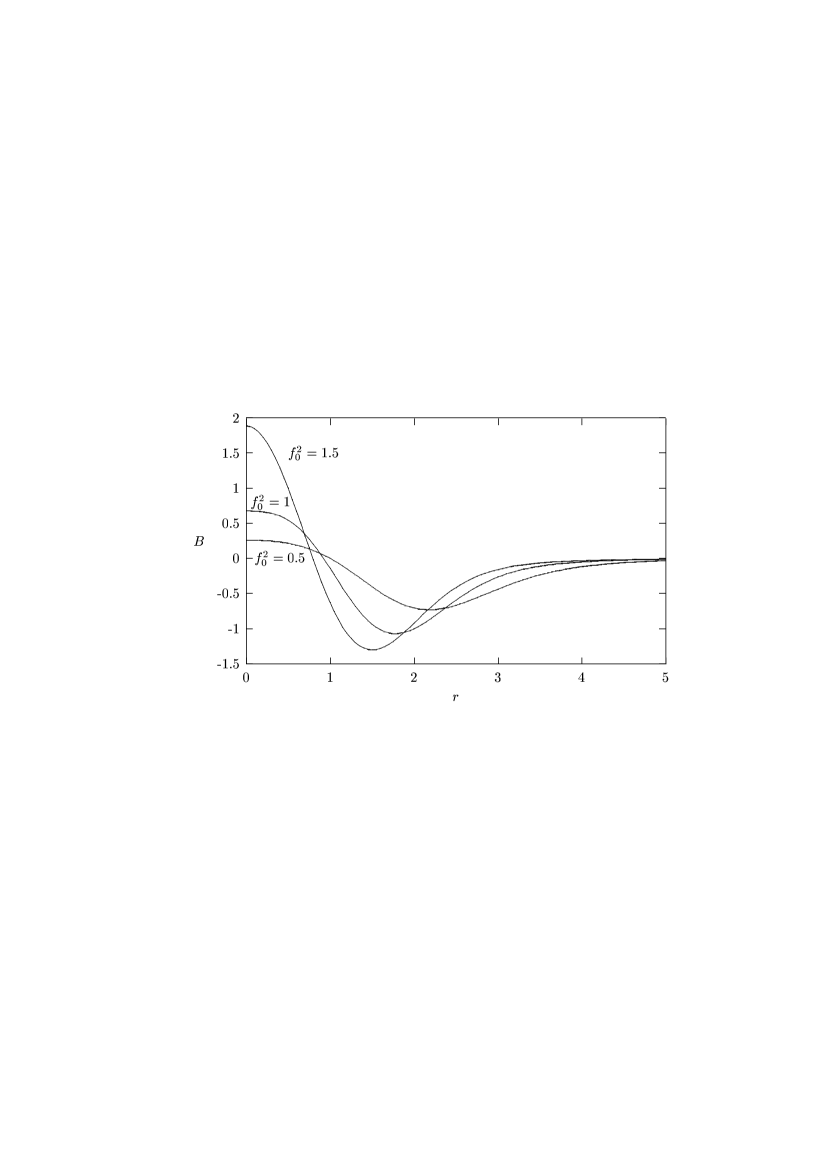
Figure 2: The magnetic field $B(r)$ for the anti-selfdual non-relativistic solution for different values of $f_{0}$. $\theta$ and $\kappa$ have been taken equal to 1.

Figure 3: The magnetic field $B(r)$ for the selfdual relativistic solution for different values of $a=v^{2}\theta/(2\kappa^{2})$.

Figure 4: The magnetic field $B(r)$ for the anti-selfdual relativistic solution for different values of $a=v^{2}\theta/(2\kappa^{2})$.

References

• [1] A.Connes, M.R. Douglas and A.S. Schwarz, JHEP 02 (1998) 003.
• [2] M.R. Douglas and C. Hull, JHEP 02 (1998) 008.
• [3] N. Seiberg and E. Witten, JHEP 09 (1999) 032.
• [4] A. Hashimoto, JHEP 9911 (1999) 005.
• [5] S. Moriyama, Phys.Lett. B485 (2000) 278.
• [6] R. Gopakumar, S. Minwalla and A. Strominger, JHEP 0005 (2000) 020.
• [7] D.J. Gross and N. Nekrasov, JHEP 0007 (2000) 034; JHEP 0010 (2000) 021; hep-th/0010090.
• [8] D.P. Jaktar, G. Mandal and S.R. Wadia, JHEP 0009 (2000) 018.
• [9] A.S. Gorsky, Y.M. Makeenko, K.G. Selivanov Phys.Lett. B492 (2000) 344.
• [10] M. Aganagic, R. Gopakumar, S. Minwalla and A. Strominger, hep-th/0009142
• [11] A.P. Polychronakos, Phys. Lett. B495 (2000) 407.
• [12] N. Nekrasov, hep-th/0010017.
• [13] J.A. Harvey, P. Kraus and F. Larsen, hep-th/0010060.
• [14] M. Hamanaka and S Terashima, hep-th/0010221
• [15] K. Hashimoto, hep-th/0010251.
• [16] D. Bak, hep-th/0008204.
• [17] D. Bak, K. Lee and J-H. Park, hep-th/0011099.
• [18] G.S. Lozano, E.F. Moreno and F.A. Schaposnik, Phys. Lett. B (in press) hep-th/0011205.
• [19] See E. Fradkin, Field Theories of Condensed Matter systems, and references therein.
• [20] See R.Jackiw in Diverse Topics in Theoretical and Mathematical Physics World Sci. Singapore, 1995, pp 465-514 and references therein.
• [21] C. Chu, Nucl. Phys. B580 (2000) 352.
• [22] A. A. Bichl, J. M. Grimstrup, V. Putz and M. Schweda, JHEP0007 (2000) 046.
• [23] G. Chen and Y. Wu, hep-th/0006114.
• [24] S. Mukhi and N. V. Suryanarayana, JHEP0011 (2000) 006.
• [25] N. Grandi and G. A. Silva, hep-th/0010113.
• [26] A. P. Polychronakos, JHEP0011 (2000) 008.
• [27] V. John, A. V. Nguyen and C. W. Kameshwar, Phys. Lett. B371 (1996) 252.
• [28] R, Jackiw and S.-Y. Pi, Phys. Rev. Lett. 64 (1990) 2969, (C) 66 (1991) 2682; Phys. Rev. D42 (1990) 3500.
• [29] J. Hong, Y. Kim and P.Y. Pac, Phys. Rev. Lett. 64 (1990) 2230.
• [30] R. Jackiw and E. Weinberg, Phys. Rev. Lett. 64 (1990) 2234; R. Jackiw, K. Lee and E. Weinberg, Phys. Rev. D42 (1990) 3488.
• [31] H. de Vega and F.A. Schaposnik, Phys. Rev. D14 (1976) 1100.
• [32] E.B. Bogomol’nyi, Sov. Jour. Nucl. Phys. 24 (1976) 449.
• [33] M. Sheikh-Jabbari, Phys. Lett. B455 (1999) 129.
• [34] D. Bigatti and L. Susskind, Phys. Rev. D62 (2000) 066004.
• [35] V. Pasquier, Phys.Lett. B490 (2000) 258.
• [36] B.A. Bernevig, J. Brodie, L. Susskind and N. Toumbas, hep-th/0010105.
• [37] S.S. Gubser and M. Rangamani, hep-th/0012155.
• [38] G. Lozano, Phys. Lett. B283 (1992) 70; O .Bergmann and G. Lozano, Ann. Phys. (N.Y.) 229 (1994) 416.
• [39] M. Chaichian, A. Demichev, P. Presnajder, M.M. Sheikh-Jabbari and A.  Tureanu, hep-th/0012175.
Refer to caption