Excited TBA Equations I:
Massive Tricritical Ising Model

Abstract

We consider the massive tricritical Ising model ${\cal M}(4,5)$ perturbed by the thermal operator $\varphi_{1,3}$ in a cylindrical geometry and apply integrable boundary conditions, labelled by the Kac labels $(r,s)$, that are natural off-critical perturbations of known conformal boundary conditions. We derive massive thermodynamic Bethe ansatz (TBA) equations for all excitations by solving, in the continuum scaling limit, the TBA functional equation satisfied by the double-row transfer matrices of the $A_{4}$ lattice model of Andrews, Baxter and Forrester (ABF) in Regime III. The complete classification of excitations, in terms of $(\boldsymbol{m},\boldsymbol{n})$ systems, is precisely the same as at the conformal tricritical point. Our methods also apply on a torus but we first consider $(r,s)$ boundaries on the cylinder because the classification of states is simply related to fermionic representations of single Virasoro characters $\chi_{r,s}(q)$. We study the TBA equations analytically and numerically to determine the conformal UV and free particle IR spectra and the connecting massive flows. The TBA equations in Regime IV and massless RG flows are studied in Part II.

1 Introduction

Ever since their introduction [1, 2, 3], Thermodynamic Bethe Ansatz (TBA) equations have been an important tool in the study of both massive and massless integrable quantum field theories. Although extensive studies have been carried out on scaling energies of vacuum or ground states only relatively few excited states [4, 5, 6, 7, 8] have proven amenable to TBA analysis and these are primarily restricted to massive and diagonal scattering theories. So despite considerable successes, the application of TBA methods has been hampered by inherent limitations. The primary obstacle is that to date there is no systematic and unified derivation of excited state TBA equations. Indeed, the current treatments of excited states are at best ad hoc and fall well short of a complete analysis of all excitations. Here we address these limitations and propose a systematic approach based on the lattice. More specifically, we will show in a series of papers that both massive and massless excited TBA equations can be systematically obtained by studying the continuum scaling limit of the associated integrable lattice models. Perhaps the most important input from the lattice approach is an insight into the analytic structure of the excited state solutions of the TBA equations. Previously this structure had to be guessed. In stark contrast, in the lattice approach, the analyticity structure can be probed by direct numerical calculations on finite size transfer matrices.

Although the methods developed in this paper are very general, for simplicity and concreteness, we consider as a first example the massive tricritical Ising model ${\cal M}(4,5)$ perturbed by the thermal operator $\varphi_{1,3}$. Although this is a non-diagonal scattering theory and more complicated from the viewpoint of integrable quantum field theory, this is the simplest case beyond the Ising model and Lee-Yang theory for analysis by the lattice approach. The integrable lattice model associated to the thermally perturbed tricritical Ising model is the interacting hard square model or generalized hard hexagon model solved by Baxter [9, 10]. This model, with its ${\mathbb{Z}}_{2}$ sublattice symmetry, is known to be in the universality class of the tricritical Ising model. More generally, this model is the special case $L=4$ of the $A_{L}$ lattice models of Andrews, Baxter and Forrester [11] with the $L=3$ model being the usual Ising model. Generically these $A_{L}$ models, with their ${\mathbb{Z}}_{2}$ height reversal symmetry, are in the universality class of multicritical Ising models. Moreover, the continuum scaling limit of the $A_{L}$ models realize [12] the $\varphi_{1,3}$ thermal perturbation of the $s\ell(2)$ unitary minimal models [13] and the ground states are described by the $A_{L-2}$ TBA equations of Zamolodchikov [3].

There have been many relevant studies of the tricritical hard square or $A_{4}$ lattice model and the more general $A_{L}$ models from the lattice viewpoint. For the $A_{4}$ model, the off-critical TBA functional equation for periodic boundary conditions has been derived and solved [14, 15] for the bulk properties and correlation lengths. The off-critical TBA functional equations for the $A_{L}$ models were derived by Klümper and Pearce [16, 17, 18]. But only the critical or “conformal TBA” equations were derived and solved in the critical scaling limit for the central charges and conformal weights. The very same off-critical TBA functional equations for $A_{L}$ models were subsequently derived [19] in the presence of integrable boundaries showing that the TBA functional equations are universal in the sense that they are independent of the boundary conditions. A biproduct of introducing boundaries is that the problem of classifying the excitations becomes much easier. This is reflected in the fact that at criticality the cylinder partition functions are given as linear forms in characters rather than the usual sesquilinear form on the torus. Indeed, by a judicious choice of $(r,s)$ boundary conditions, the cylinder partition function is just a single Virasoro character $\chi_{r,s}(q)$ and the complete classification of excitations [20] in terms of $(\boldsymbol{m},\boldsymbol{n})$ systems [21, 22] is related to a fermionic representation of the character $\chi_{r,s}(q)$. This simplification enabled [20] the complete analytic calculation of the conformal cylinder partition functions of the $A_{4}$ model with 6 different conformal boundary conditions $(r,s)$ which are conjugate to the 6 primary fields of the tricritical Ising conformal field theory. The generalization of these results to the critical $A_{L}$ lattice models with $(r,s)$ boundaries is currently in progress [23].

In 1998, Pearce and Nienhuis [24] analysed the off-critical continuum scaling limit of the TBA functional equations for the $A_{L}$ lattice models to derive from the lattice the full set of massive and massless $A_{L-2}$ ground state TBA equations conjectured by Zamolodchikov. The scale parameter $mR$ is simply related to the scaling limit of lattice parameters by

$$\mu=\frac{mR}{4}=\lim_{N\to\infty,\,t\to 0}Nt^{\nu}$$ (1.1)

or more precisely

$$R=\lim_{N\to\infty,\,a\to 0}Na,\qquad m=\lim_{t\to 0,\,a\to 0}\frac{4t^{\nu}}{a}$$ (1.2)

where $a$ is the lattice spacing, $m$ is a mass, $R$ is the continuum length scale, $\nu=(L+1)/4$ is the correlation length exponent and $t=p^{2}$ is the deviation from critical temperature variable with $p$ the elliptic nome appearing in the Boltzmann weights of the $A_{L}$ models.

Our primary goal in this series of papers is to extend the analysis of Pearce and Nienhuis to all excitations of the $A_{4}$ model both in the massive and massless regimes. This entails perturbing the analysis of O’Brien, Pearce and Warnaar [20] off criticality. To handle the problem of classification of all the excitations it is easier to introduce boundaries and to work on the cylinder even though a study of boundary properties is not our primary goal. Our immediate goal is to study the flow of excitation energies from the UV ($R=0$) to the IR ($R\to\infty$) limit. In the massive case we are thus able to compile the conformal-massive dictionary that eluded Melzer [25]. In the massless case considered in paper II [26], we follow the renormalization group flow from the tricritical to the critical Ising model fixed points. This leads to a flow between the characters of these theories.

In this paper we consider just the massive regime. The layout of the paper is as follows. In Section 2 we define the $A_{4}$ lattice model. We then describe the classification of excitations and discuss their unique labelling in terms of quantum numbers. This classification is in fact identical to the classification [20] at the tricritical point. In Section 3 we present the derivation of the off-critical massive TBA equations. The numerical solution of these equations is presented in Section 4. Throughout we concentrate on the three $(r,s)$ boundary conditions with $s=1$ rather than presenting exhaustive results for the six distinct $(r,s)$ boundary conditions. We believe these results are indicative of what can be achieved. While the calculations are similar for the other boundary conditions, we point out that in some cases there are further subtleties related to the appearance of frozen zeros. We conclude with a general discussion.

2 Lattice Approach

2.1 $A_{4}$ lattice model

The $A_{4}$ RSOS lattice model is defined on a square lattice with spins or heights $a=1,2,3,4$ restricted so that nearest neighbour heights differ by $\pm 1$. This model corresponds to the special case $L=4$ of the $A_{L}$ RSOS models of Andrews, Baxter and Forrester [11] with spins $a=1,\ldots,L$ and Boltzmann weights ($\lambda=\pi/5$ for the $A_{4}$ model)

$$W\!\!\left.\left(\begin{matrix}a\pm 1&a\\ a&a\mp 1\end{matrix}\right|u\right) = \frac{\vartheta_{1}(\lambda-u)}{\vartheta_{1}(\lambda)}$$ (2.1)

$$W\!\!\left.\left(\begin{matrix}a&a\pm 1\\ a\mp 1&a\end{matrix}\right|u\right) = \left(\frac{\vartheta_{1}((a-1)\lambda)\vartheta_{1}((a+1)\lambda)}{\vartheta_{1}^{2}(a\lambda)}\right)^{1/2}\,\frac{\vartheta_{1}(u)}{\vartheta_{1}(\lambda)}$$ (2.2)

$$W\!\!\left.\left(\begin{matrix}a&a\pm 1\\ a\pm 1&a\end{matrix}\right|u\right) = \frac{\vartheta_{1}(a\lambda\pm u)}{\vartheta_{1}(a\lambda)}.$$ (2.3)

Here $u$ is the spectral parameter, $\lambda=\pi/(L+1)$ is the crossing parameter and $\vartheta_{1}(u)=\vartheta_{1}(u,p)$ is one of the standard elliptic theta functions as given in Gradshteyn and Ryzhik [27]

$$\vartheta_{1}(u,p) = 2p^{1/4}\sin u\prod_{n=1}^{\infty}(1-2p^{2n}\cos 2u+p^{4n})(1-p^{2n})$$ (2.4)

$$\vartheta_{2}(u,p) = 2p^{1/4}\cos u\prod_{n=1}^{\infty}(1+2p^{2n}\cos 2u+p^{4n})(1-p^{2n})$$ (2.5)

$$\vartheta_{3}(u,p) = \prod_{n=1}^{\infty}(1+2p^{2n-1}\cos 2u+p^{2(2n-1)})(1-p^{2n})$$ (2.6)

$$\vartheta_{4}(u,p) = \prod_{n=1}^{\infty}(1-2p^{2n-1}\cos 2u+p^{2(2n-1)})(1-p^{2n}).$$ (2.7)

Integrability derives from the fact that these local face weights satisfy the Yang-Baxter equation.

The elliptic nome $p$ is a temperature-like variable. The $A_{L}$ lattice models are critical for $p=0$ and off-critical for $p\neq 0$ so we introduce the deviation from critical temperature variable $t=p^{2}$. There are four distinct off-critical physical regimes depending on the sign of $u$ and $t$:

$$\begin{array}[]{lcr}\text{Regime I:}&\qquad-\pi/2+\lambda\leq u\leq 0,&-1<t<0\phantom{.}\\ \text{Regime II:}&-\pi/2+\lambda\leq u\leq 0,&0<t<1\phantom{.}\\ \text{Regime III:}&0\leq u\leq\lambda,&0<t<1\phantom{.}\\ \text{Regime IV:}&0\leq u\leq\lambda,&-1<t<0.\end{array}$$ (2.12)

It is convenient to express the nome $p$ in terms of a real parameter $\varepsilon>0$ by

$$p=\begin{cases}e^{-\pi\varepsilon},&\text{Regimes II and III}\\ ie^{-\pi\varepsilon},&\text{Regimes I and IV}\end{cases}$$ (2.13)

so that $|p|\leq 1$ and

$$t=p^{2}=\pm\exp(-2\pi\varepsilon).$$ (2.14)

In particular, the elliptic $\vartheta_{1}$ functions satisfy the quasiperiodicity properties

$$\vartheta_{1}(u+\pi,p)=-\vartheta_{1}(u,p)$$ (2.15)

$$\vartheta_{1}(u-i\log p,p)=-p^{-1}e^{-2iu}\vartheta_{1}(u,p).$$ (2.16)

Regimes III and IV are of interest in this series of papers since they are associated, in the continuum scaling limit, with the massive and massless thermal perturbations of the unitary minimal models respectively. In Regime III, considered in this paper, $p$ is real whereas in Regime IV $p$ is pure imaginary. Regimes I and II relate to ${\mathbb{Z}}_{L-1}$ parafermions and so are not considered here.

Although we will not use it in this paper, an alternative formulation of the $A_{4}$ model is the particle or $T_{2}$ tadpole representation as shown in Figure 1. This formulation is obtained by folding the $A_{4}$ diagram and identifying the states related by the ${\mathbb{Z}}_{2}$ height reversal symmetry. More specifically, we can identify the states $a=1,4$ with $\mu=1$ and regard this as indicating the presence of a particle or an occupied site and we can identify the states $a=2,3$ with $\mu=0$ and regard this as indicating the absence of a particle or a vacant site. Once we fix the sublattice of the square lattice which has odd heights, the identification of height and particle states is a one-to-one correspondence. The adjacency constraint on the heights of the $A_{4}$ model translates into the exclusion of simultaneous occupancy of adjacent sites by particles. In this way the particle representation is seen to be equivalent to a model of interacting hard squares on the square lattice. The Boltzmann weights of this hard square model are simply given by replacing the heights $a=1,2,3,4$ by the corresponding particle occupation numbers $\mu=0,1$.

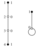
Figure 1: $A_{4}$ and $T_{2}$ graphs of allowed neighboring states for the $A_{4}$ lattice model and its particle (hard square) representation.

The isotropic phase diagram of the $A_{4}$ or interacting hard square model is shown in Figure 2 alongside the corresponding renormalization group flow in the continuum scaling limit about the tricritical point. The continuum scaling limits in Regimes III and IV give rise to the massive and massless flows respectively where the perturbation parameter is $mR$ or $\mu$.

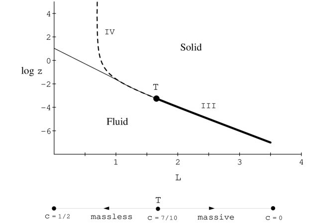
Figure 2: Isotropic phase diagram of the $A_{4}$ or interacting hard square model showing the phase boundary (solid and thick solid curves) between the fluid and square ordered solid phases. The fugacity of the particles is $z$ and $L$ is the attraction between particles. The tricritical point $T$ separates the line of Ising critical points (solid curve) from the first-order line (thick solid curve, Regime III). The model is exactly solvable on the first-order line and its analytic continuation (dashed line, Regime IV). The exact solution curve and Ising critical line are tangential at $T$. The renormalization group flow in the continuum scaling limit about the tricritical point $T$ is shown below for comparison. The central charge $c$ is indicated at the tricritical, critical and trivial fixed points.

2.2 Double row transfer matrices

To ensure integrability of the $A_{4}$ model in the presence of a boundary [19] we need commuting double row transfer matrices and triangle boundary weights which satisfy the boundary Yang-Baxter equation. The triangle weights for the $(r,s)$ boundary condition with $1\leq r\leq 3$ and $1\leq s\leq 4$ are given by

$$\begin{split}K\left(\left.\begin{matrix}r\\ r\end{matrix}\ \;r\pm 1\right|u,\xi_{L}\right)&=\left(\frac{\vartheta_{1}((r\pm 1)\lambda)}{\vartheta_{1}(r\lambda)}\right)^{\frac{1}{2}}\dfrac{\vartheta_{1}(u\pm\xi_{L})\vartheta_{1}(u\mp r\lambda\mp\xi_{L})}{\vartheta_{1}^{2}(\lambda)}\\ K\left(\left.s\pm 1\ \;\begin{matrix}s\\ s\end{matrix}\right|u,\xi_{R}\right)&=\left(\frac{\vartheta_{1}((s\pm 1)\lambda)}{\vartheta_{1}(s\lambda)}\right)^{\frac{1}{2}}\dfrac{\vartheta_{4}(u\pm\xi_{R})\vartheta_{4}(u\mp s\lambda\mp\xi_{R})}{\vartheta_{4}^{2}(\lambda)}.\end{split}$$ (2.17)

The parameters $\xi_{L},\xi_{R}$ are arbitrary and can be taken to be complex, however here we restrict them to the real interval $(\lambda/2,\lambda)$. To obtain conformal boundary conditions at the isotropic tricritical point $u=\lambda/2$, $t=p=0$ we should choose [28] $\xi_{L}=\xi_{R}=\lambda/2$. Integrability in the presence of these boundaries derives from the fact that these boundary triangle weights satisfy the boundary Yang-Baxter equation.

The face and triangle boundary weights are used to construct [19] a family of commuting double row transfer matrices $\boldsymbol{D}(u)$. For a lattice of width $N$, the entries of $\boldsymbol{D}(u)$ are given diagrammatically by

$$\boldsymbol{D}(u)_{\boldsymbol{a},\boldsymbol{b}}=\sum_{c_{0},\dots,c_{N}}\raisebox{-55.76714pt}[51.78412pt][43.81747pt]{\begin{picture}(6.4,2.4)(0.4,0.1)\put(0.5,0.5){\line(0,1){2.0}}\put(6.5,0.5){\line(0,1){2.0}} \put(1.0,0.5){\line(0,1){2.0}}\put(2.0,0.5){\line(0,1){2.0}}\put(3.0,0.5){\line(0,1){2.0}} \put(5.0,0.5){\line(0,1){2.0}}\put(6.0,0.5){\line(0,1){2.0}} \put(1.0,0.5){\line(1,0){5.0}}\put(1.0,1.5){\line(1,0){5.0}}\put(1.0,2.5){\line(1,0){5.0}} \put(1.0,1.5){\line(-1,2){0.5}}\put(1.0,1.5){\line(-1,-2){0.5}} \put(6.0,1.5){\line(1,2){0.5}}\put(6.0,1.5){\line(1,-2){0.5}} \put(0.5,0.45){\makebox(0.0,0.0)[t]{${\scriptstyle r}$}}\put(1.0,0.45){\makebox(0.0,0.0)[t]{${\scriptstyle r}$}} \put(2.0,0.45){\makebox(0.0,0.0)[t]{${\scriptstyle a_{1}}$}}\put(3.0,0.45){\makebox(0.0,0.0)[t]{${\scriptstyle a_{2}}$}} \put(5.0,0.45){\makebox(0.0,0.0)[t]{${\scriptstyle a_{N-1}}$}}\put(6.0,0.45){\makebox(0.0,0.0)[t]{${\scriptstyle s}$}} \put(6.5,0.45){\makebox(0.0,0.0)[t]{${\scriptstyle s}$}} \put(0.5,2.6){\makebox(0.0,0.0)[b]{${\scriptstyle r}$}}\put(1.0,2.6){\makebox(0.0,0.0)[b]{${\scriptstyle r}$}} \put(2.0,2.6){\makebox(0.0,0.0)[b]{${\scriptstyle b_{1}}$}}\put(3.0,2.6){\makebox(0.0,0.0)[b]{${\scriptstyle b_{2}}$}} \put(5.0,2.6){\makebox(0.0,0.0)[b]{${\scriptstyle b_{N-1}}$}}\put(6.0,2.6){\makebox(0.0,0.0)[b]{${\scriptstyle s}$}} \put(6.5,2.6){\makebox(0.0,0.0)[b]{${\scriptstyle s}$}} \put(1.05,1.45){\makebox(0.0,0.0)[tl]{${\scriptstyle c_{0}}$}}\put(2.05,1.45){\makebox(0.0,0.0)[tl]{${\scriptstyle c_{1}}$}} \put(3.05,1.45){\makebox(0.0,0.0)[tl]{${\scriptstyle c_{2}}$}}\put(4.99,1.45){\makebox(0.0,0.0)[tr]{${\scriptstyle c_{N-1}}$}} \put(5.99,1.45){\makebox(0.0,0.0)[tr]{${\scriptstyle c_{N}}$}} \put(1.5,1.0){\makebox(0.0,0.0)[]{$u$}}\put(2.5,1.0){\makebox(0.0,0.0)[]{$u$}}\put(5.5,1.0){\makebox(0.0,0.0)[]{$u$}} \put(1.5,2.0){\makebox(0.0,0.0)[]{$\lambda\!-\!u$}}\put(2.5,2.0){\makebox(0.0,0.0)[]{$\lambda\!-\!u$}} \put(5.5,2.0){\makebox(0.0,0.0)[]{$\lambda\!-\!u$}} \put(0.71,1.5){\makebox(0.0,0.0)[]{$\lambda\!-\!u\ \ \ $}}\put(6.29,1.5){\makebox(0.0,0.0)[]{$u$}} \put(0.5,0.5){\makebox(0.5,0.0)[]{\dotfill}}\put(0.5,2.5){\makebox(0.5,0.0)[]{\dotfill}} \put(6.0,0.5){\makebox(0.5,0.0)[]{\dotfill}}\put(6.0,2.5){\makebox(0.5,0.0)[]{\dotfill}} \end{picture}}$$ (2.18)

It is further convenient to define the normalized transfer matrix

$$\boldsymbol{t}(u)=S_{r,s}(u)S(u)\Bigl{[}i\,\frac{\vartheta_{1}(u+2\lambda,p)\vartheta_{1}(\lambda,p)}{\vartheta_{1}(u+3\lambda,p)\vartheta_{1}(u+\lambda,p)}\Bigr{]}^{2N}\boldsymbol{D}(u)$$ (2.19)

where

$$S(u)=\frac{\vartheta_{1}(2u-\lambda,p)^{2}}{\vartheta_{1}(2u-3\lambda,p)\vartheta_{1}(2u+\lambda,p)}$$ (2.20)

and

$$S_{r,s}(u)=(-1)^{s}h_{r}(u-\xi_{L})h_{-r}(u+\xi_{L})\bar{h}_{s}(u-\xi_{R})\bar{h}_{-s}(u+\xi_{R})$$ (2.21)

with

$$h_{r}(u) =\frac{\vartheta_{1}(\lambda,p)\vartheta_{1}(u+(3-r)\lambda,p)\vartheta_{1}(u+(1-r)\lambda,p)}{\vartheta_{1}(u,p)\vartheta_{1}(u-\lambda,p)\vartheta_{1}(u+2\lambda,p)}$$ (2.22)

$$\bar{h}_{s}(u) =\frac{\vartheta_{4}(\lambda,p)\vartheta_{4}(u+(3-s)\lambda,p)\vartheta_{4}(u+(1-s)\lambda,p)}{\vartheta_{4}(u,p)\vartheta_{4}(u-\lambda,p)\vartheta_{4}(u+2\lambda,p)}.$$ (2.23)

It can then be shown [19] that the normalized transfer matrix satisfies the universal TBA functional equation

$$\boldsymbol{t}(u)\boldsymbol{t}(u+\lambda)=\boldsymbol{I}+\boldsymbol{t}(u+3\lambda)$$ (2.24)

independent of the boundary condition $(r,s)$. This is precisely the same TBA functional equation that holds in the periodic case [14]. Since the transfer matrices commute this functional equations also holds for each eigenvalue $t(u)$ of $\boldsymbol{t}(u)$.

The TBA functional equations will be solved for the finite-size corrections to the eigenvalues $D(u)$ of the double row transfer matrices $\boldsymbol{D}(u)$. In the scaling limit, the finite-size corrections to the eigenvalues $D(u)$ are related to the excitation energies $E(R)$ of the associated perturbed conformal field theory by

$$-\mbox{$\textstyle{1\over 2}$}\log D(u)=Nf_{\text{bulk}}(u)+b_{r,s}(u)+\frac{R\sin\vartheta}{N}\,E(R)+o(\frac{1}{N})$$ (2.25)

where $f_{\text{bulk}}(u)$ is the bulk free energy, $b_{r,s}(u)$ is the boundary free energy and the anisotropy angle is given by

$$\vartheta=\begin{cases}(L+1)u,&\text{Regimes III and IV}\\ -\displaystyle{\frac{2(L+1)u}{L-1}},&\text{Regimes I and II.}\end{cases}$$ (2.26)

Depending on the boundary conditions, the boundary free energy $b_{r,s}(u)$ may contain an interfacial free energy contribution. The bulk and boundary free energies can be calculated [29, 30, 31] by the inversion relation method. Despite the appearance of $1/N$ corrections, the system is not in general conformally invariant. The system is conformal however at critical points which can occur in the ultraviolet ($R\to 0$) and infrared ($R\to\infty$) limits with

$$\frac{RE(R)}{2\pi}\to-\frac{c}{24}+\Delta_{r,s}+n,\qquad n\in{\mathbb{N}}$$ (2.27)

where $c$ is the central charge of the appropriate conformal field theory, $\Delta_{r,s}$ are the related conformal weights and $n=0,1,\ldots$ labels the tower of descendants. The largest eigenvalue occurs for the vacuum or ground state with the boundary condition $(r,s)=(1,1)$. In this case $\Delta_{1,1}=0$ and $n=0$. The massive $R\to\infty$ scaling limit in Regime III, however, is trivial in the sense that for this ground state $RE(R)\to 0$ corresponding to $c=0$ and the scattering of free massive particles.

2.3 Classification: $(\boldsymbol{m},\boldsymbol{n})$ systems and quantum numbers

TBA functional equations admit infinite families of solutions for the eigenvalues $t(u)$. The analyticity properties are therefore crucial in selecting out the required solutions. The transfer matrix eigenvalues $D(u)$ are entire functions of $u$ and are characterised (up to an overall constant) by their zeros in the complex $u$ plane. It is precisely at these zeros that $\log t(u)$ is non-analytic but analyticity of $\log t(u)$ is required to solve the TBA functional equations by Fourier series. From quasiperiodicity, the matrix $\boldsymbol{t}(u)$ and eigenvalues $t(u)$ are doubly periodic. It follows that the eigenvalues $t(u)$ are doubly periodic meromorphic functions. It is convenient to fix the period rectangles as

$$\text{period rectangle}=\begin{cases}(-\frac{\lambda}{2},\frac{9\lambda}{2})\times(-\frac{\pi i\varepsilon}{2},\frac{\pi i\varepsilon}{2}),&\text{Regime~{}III}\\ (-\frac{\lambda}{2},\frac{9\lambda}{2})\times(-\pi i\varepsilon,\pi i\varepsilon),&\text{Regime~{}IV}\end{cases}$$ (2.28)

so we then only need to consider the analyticity inside these period rectangles. In Regime IV there is an additional symmetry within the period rectangle

$$t(u\pm\pi/2+\pi i\varepsilon)=t(u)$$ (2.29)

so we can restrict ourselves further to the rectangle $(-\frac{\lambda}{2},2\lambda)\times(-\pi i\varepsilon,\pi i\varepsilon)$. The normalization factors relating $D(u)$ to $t(u)$ only introduce extra zeros and poles on the real axis. Since $\boldsymbol{D}(u)$ is real symmetric for real $u$, that is $\boldsymbol{D}(u)=\boldsymbol{D}(u)^{T}$, it follows that, for any eigenvalue $D(u)$ or $t(u)$, the distribution of zeros in the upper and lower half planes are identical and simply related by complex conjugation. It is therefore sufficient to classify the eigenvalues by the patterns of zeros in the upper half period rectangle.

It turns out that in Regime III the pattern of zeros inside the periodic rectangle is qualitatively the same as in the critical case. This was observed by direct numerical diagonalization of a sequence of finite-size transfer matrices approaching the scaling limit $N\to\infty$, $t\to 0$ for modest sizes of $N$. As a consequence, in Regime III we can use the known classification [20] of eigenvalues at the tricritical point ($R=0$) in terms of $(\boldsymbol{m},\boldsymbol{n})$ systems and this classification will apply for any $R$ in the range $0\leq R<\infty$. This simplifying feature does not hold in the massless Regime IV where in stark contrast some of the patterns of zeros qualitatively change under the flow as $R$ increases [26]. Since the classification of excitations in Regime III of interest here is the same as at the tricritical point we summarise the salient features of this classification here. We limit discussion to the boundary condition $(r,s)=(1,1)$. The other cases are similar [20] although in some cases it is necessary to introduce two $(\boldsymbol{m},\boldsymbol{n})$ systems for a given $(r,s)$ boundary condition.

The analyticity properties of $D(u)$ are relevant in the two analyticity strips

$$-\frac{\lambda}{2}<\mbox{Re}(u)<\frac{3\lambda}{2},\qquad 2\lambda<\mbox{Re}(u)<4\lambda$$ (2.30)

We refer to these as strip 1 and 2 respectively and label them by $i=1,2$. Since the Boltzmann weights are real and positive for $0<u<\lambda$, strip 1 is referred to as the physical analyticity strip. From direct numerical diagonalization of $\boldsymbol{D}(u)$ with the $(1,1)$ boundary condition we observe that, apart from a pair of zeros on the real axis at $u=\lambda+\xi$ and $u=5\lambda-\xi$ induced by the left boundary triangle weight, each eigenvalue has zeros on the lines $\mbox{Re}(u)=-\lambda/2,\,\lambda/2,\,3\lambda/2,\,2\lambda,\,4\lambda$ corresponding to the edges and center lines of the two analyticity strips. Specifically, $1$-strings and $2$-strings occur in strip 1 and 2. A $1$-string is given by a single zero $u_{j}$ in the center of a strip such that

$$\mbox{Re}(u_{j})=\begin{cases}\lambda/2,&\text{strip 1}\\ 3\lambda,&\text{strip 2.}\end{cases}$$ (2.31)

A $2$-string is a pair of zeros $(u_{j},u^{\prime}_{j})$ on the edge of a strip with equal imaginary part and

$$(\mbox{Re}(u_{j}),\mbox{Re}(u^{\prime}_{j}))=\begin{cases}(-\lambda/2,3\lambda/2),&\text{strip 1}\\ (2\lambda,4\lambda),&\text{strip 2.}\end{cases}$$ (2.32)

Distributions of zeros for two typical eigenvalues of $D(u)$ for $N=16$ are depicted in Figures 3 and 4.

Figure 3: Zeros within a period rectangle in the complex $u$-plane of the largest eigenvalue of $D(u)$ with string content $m_{1}=6$, $n_{1}=3$, $m_{2}=2$, $n_{2}=1$.

Figure 4: Zeros within a period rectangle in the complex $u$-plane of another typical eigenvalue of $D(u)$ with string content $m_{1}=6$, $n_{1}=3$, $m_{2}=2$, $n_{2}=1$. This pattern of zeros is obtained by permuting the ordering of the 1-strings and 2-strings within each strip of Figure 3.

We note that for finite $N$ the $2$-strings do not fall precisely on the lines given in equation (2.32), but that this deviation decreases exponentially, that is as $|\delta|^{N}$ with $|\delta|<1$, as $N$ increases. These patterns are consistent with the crossing $\boldsymbol{D}(u)=\boldsymbol{D}(\lambda-u)$ and transpose $\boldsymbol{D}(u)=\boldsymbol{D}(u)^{T}$ symmetry of the double row transfer matrix.

Given an eigenvalue, we denote the number of strings in the upper half period rectangle as follows:

$$\begin{split}m_{i}&=\text{number of $1$-strings in strip $i=1,2$}\\ n_{i}&=\text{number of $2$-strings in strip $i=1,2$}.\end{split}$$ (2.33)

The relations [20] between these numbers determining the string content take the form of an $(\boldsymbol{m},\boldsymbol{n})$-system [21, 22]

$$\boldsymbol{m}+\boldsymbol{n}=\frac{1}{2}(N\boldsymbol{e}_{1}+\mathcal{I}\boldsymbol{m})$$ (2.34)

where $\boldsymbol{m}=(m_{1},m_{2})$, $\boldsymbol{n}=(n_{1},n_{2})$, $\boldsymbol{e}_{1}=(1,0)$, and $\mathcal{I}$ is the $\mathrm{A}_{2}$ incidence matrix with entries $\mathcal{I}_{j,k}=\delta_{|j-k|,1}$. Clearly here we require that $m_{1},m_{2}$ and $N$ are even. For the leading excitations $m_{1},m_{2},n_{2}$ are finite but $n_{1}\sim N/2$ as $N\to\infty$. Indeed, the vacuum or ground state is given by $m_{1}=m_{2}=n_{2}=0$ and $n_{1}=N/2$.

For each system size $N$, there are many eigenvalues with the same string content $(\boldsymbol{m},\boldsymbol{n})$. These eigenvalues are distinguished by the relative vertical orderings of the $1$ and $2$-strings within the period rectangle along each strip. Denoting the imaginary parts of the $1$-strings in strip $i$ by $0<v_{1}^{(i)}<\dots<v_{m_{i}}^{(i)}$, and the imaginary parts of the $2$-strings in strip $i$ by $0<w_{1}^{(i)}<\dots<w_{n_{i}}^{(i)}$, we see that in Figure 3

$$\begin{gathered}0<w_{1}^{(1)}<w_{2}^{(1)}<w_{3}^{(1)}<v_{1}^{(1)}<v_{2}^{(1)}<\dots<v_{6}^{(1)}\\ 0<w_{1}^{(2)}<v_{1}^{(2)}<v_{2}^{(2)}\end{gathered}$$ (2.35)

whereas in Figure 4, which has the same string content,

$$\begin{gathered}0<w_{1}^{(1)}<v_{1}^{(1)}<v_{2}^{(1)}<w_{2}^{(1)}<v_{3}^{(1)}<w_{3}^{(1)}<v_{4}^{(1)}<v_{5}^{(1)}<v_{6}^{(1)}\\ 0<v_{1}^{(2)}<w_{1}^{(2)}<v_{2}^{(2)}.\end{gathered}$$ (2.36)

Notice that the 1-strings $v_{j}^{(i)}$ and 2-strings $w_{j}^{(i)}$ labelled by $j=1$ are closest to the real axis. Clearly, the total number of possible orderings for a given string content $(\boldsymbol{m},\boldsymbol{n})$ is $\binom{m_{1}+n_{1}}{m_{1}}\binom{m_{2}+n_{2}}{m_{2}}$. Summing over all allowed string contents $(\boldsymbol{m},\boldsymbol{n})$ using (2.34) then gives

$$\sum_{(\boldsymbol{m},\boldsymbol{n})}\binom{m_{1}+n_{1}}{m_{1}}\binom{m_{2}+n_{2}}{m_{2}}=A^{N}_{1,1}.$$ (2.37)

This is indeed the correct number of eigenvalues as given by the dimension of the double row transfer matrix, which is $A^{N}_{1,1}$, the number of $N$-step paths from 1 to 1, where $A$ is the $A_{4}$ adjacency matrix.

In the scaling limit

$$\mu=\frac{mR}{4}=\lim_{N\to\infty,\;t\to 0}N\,t^{5/4}$$ (2.38)

the positions of the 1- and 2-strings grow logarithmically as

$$v^{(i)}_{j},w^{(i)}_{j}\,\sim\,-\frac{1}{4}\log t+\mbox{const}\,=\,\frac{1}{5}\log N-\frac{1}{5}\log\mu+\mbox{const}.$$ (2.39)

More specifically, we define the scaled locations of the strings in strips $i=1,2$ as

$$\begin{split}\beta^{(i)}_{j}&=\lim_{N\to\infty,\,t\to 0}\left(5v^{(i)}_{j}+\frac{5}{4}\log t\right),\qquad j=1,2,\dots,m_{1}\\ \gamma^{(i)}_{k}&=\lim_{N\to\infty,\,t\to 0}\left(5w^{(i)}_{k}+\frac{5}{4}\log t\right),\qquad k=1,2,\dots,m_{2}\end{split}$$ (2.40)

An excitation with string content $(\boldsymbol{m},\boldsymbol{n})$ is uniquely labelled by a set of quantum numbers

$$I=(I^{(1)}|I^{(2)})=(I_{1}^{(1)},I_{2}^{(1)},\ldots,I_{m_{1}}^{(1)}\;|\;I_{1}^{(2)},I_{2}^{(2)},\ldots,I_{m_{2}}^{(2)})$$ (2.41)

where the integers $I_{j}^{(i)}\in{\mathbb{N}}$ with $i=1,2$ give the number of 2-strings whose imaginary parts $w_{k}^{(i)}$ are greater than that of the given 1-string $v_{j}^{(i)}$. Clearly, the quantum numbers $I^{(j)}_{k}$ satisfy

$$n_{j}\geq I^{(j)}_{1}\geq I^{(j)}_{2}\geq\dots\geq I^{(j)}_{m_{j}}\geq 0\qquad i=1,2.$$ (2.42)

Conversely, given the quantum numbers we can read off the values of $m_{1}$ and $m_{2}$ and then $n_{1}$ and $n_{2}$ are uniquely determined by the $(\boldsymbol{m},\boldsymbol{n})$ system. For given string content $(\boldsymbol{m},\boldsymbol{n})$, the lowest excitation occurs when all of the 1-strings are further out from the real axis than all of the 2-strings. In this case all of the quantum numbers vanish $I_{j}^{(i)}=0$. Bringing the location of a 1-string closer to the real axis by interchanging the location of the 1-string with a 2-string increments its quantum number by one unit and increases the energy. At the tricritical point where $R=0$ these jumps in energy are quantised in a tower with energy levels given by [20]

$$E=\lim_{R\to 0}\frac{RE(R)}{2\pi}=-\frac{c}{24}+\frac{1}{4}\boldsymbol{m}C\boldsymbol{m}+\sum_{i=1}^{2}\sum_{j=1}^{m_{i}}I^{(i)}_{j}.$$ (2.43)

Here $C$ is the $A_{2}$ Cartan matrix and the central charge is $c=7/10$.

More succinctly, the generating function for the finite-size spectra of a cylindrical lattice built by $M$ applications of the double row transfer matrix with $(1,1)$ boundary condition is given by a finitized Virasoro character [21, 22]

$$Z_{(1,1)}^{(N)}(q)=\sum_{E}q^{E}=q^{-c/24}\sum_{(\boldsymbol{m},\boldsymbol{n})}q^{\frac{1}{4}\boldsymbol{m}C\boldsymbol{m}}\genfrac{[}{]}{0.0pt}{}{m_{1}+n_{1}}{m_{1}}\genfrac{[}{]}{0.0pt}{}{m_{2}+n_{2}}{m_{2}}=\chi_{1,1}^{(N)}(q)$$ (2.44)

where the sum is over the finite $(\boldsymbol{m},\boldsymbol{n})$ system, $q$ is the modular parameter

$$q=e^{-2\pi\frac{M}{N}\sin\vartheta}$$ (2.45)

and $M/N$ is the aspect ratio of the lattice. In the isotropic case when $u=\lambda/2$, the anistropy angle $\vartheta=\pi/2$ and the geometric factor $\sin\vartheta=1$. The $q$-binomial or Gaussian polynomial is defined by

$$\genfrac{[}{]}{0.0pt}{}{m+n}{m}=\sum_{I_{1}=0}^{n}\sum_{I_{2}=0}^{I_{1}}\cdots\sum_{I_{m}=0}^{I_{m-1}}q^{I_{1}+\ldots+I_{m}}=\begin{cases}\dfrac{(q)_{m+n}}{(q)_{m}(q)_{n}},&\quad m,n\geq 0\\ 0,&\quad\text{otherwise}\\ \end{cases}$$ (2.46)

with the $q$-factorials $(q)_{m}=(1-q)\cdots(1-q^{m})$ for $m\geq 1$ and $(q)_{0}=1$. In the limit $q\to 1$ the $q$-binomials reduce to the usual binomial coefficients and the partition function just counts the number of states as in (2.37). Note also that

$$\lim_{n\to\infty}\genfrac{[}{]}{0.0pt}{}{m+n}{m}=\genfrac{[}{]}{0.0pt}{}{\infty}{m}=\frac{1}{(q)_{m}}.$$ (2.47)

After using the $(\boldsymbol{m},\boldsymbol{n})$ system to eliminate $n_{1}$ and $n_{2}$, the finitized character gives the fermionic representation of the usual Virasoro character in the limit $N\to\infty$

$$\lim_{N\to\infty}\chi_{1,1}^{(N)}(q)=q^{-c/24}\sum_{m_{1},\,m_{2}\,\text{even}}\frac{q^{\frac{1}{4}\boldsymbol{m}C\boldsymbol{m}}}{(q)_{m_{1}}}\,\genfrac{[}{]}{0.0pt}{}{\frac{1}{2}m_{1}}{m_{2}}=\chi_{1,1}(q).$$ (2.48)

More generally, as explained in [20], the finitized partition functions for $(r,s)$ boundary conditions at $R=0$ are given in terms of finitized characters

$$Z_{(r,s)}^{(N)}(q)=q^{-\frac{c}{24}+\Delta_{r,s}-\frac{1}{4}(s-r)(s-r-1)}\sum_{(\boldsymbol{m},\boldsymbol{n})}q^{\frac{1}{4}\boldsymbol{m}C\boldsymbol{m}-\frac{1}{2}m_{s-1}}\prod_{i=1,2}\genfrac{[}{]}{0.0pt}{}{m_{i}+n_{i}}{m_{i}}=\chi_{r,s}^{(N)}(q)$$ (2.49)

where the $(\boldsymbol{m},\boldsymbol{n})$ system for the $(r,s)$ boundary condition is

$$\boldsymbol{m}+\boldsymbol{n}=\frac{1}{2}(N\boldsymbol{e}_{1}+\mathcal{I}\boldsymbol{m}+\boldsymbol{e}_{s-1}+\boldsymbol{e}_{4-r}).$$ (2.50)

Hence in the limit $N\to\infty$ we recover the known conformal cylinder partition functions in terms of Virasoro characters

$$Z_{r,s}(q)=\lim_{N\to\infty}\chi_{r,s}^{(N)}(q)=\chi_{r,s}(q).$$ (2.51)

3 TBA Equations in Regime III

3.1 Sector $(r,s)=(1,1)$

In this section we derive the TBA equations for the $(r,s)=(1,1)$ boundary by solving the TBA functional equations in the scaling limit for even $N$. We follow closely the derivations in [20] and [24]. The derivation for other boundary conditions is similar. We begin by factorizing $t(u)$ for large $N$ as

$$t(u)=f(u)g(u)l(u)$$ (3.1)

where $f(u)$ accounts for the bulk order-$N$ behaviour, $g(u)$ the order-$1$ boundary contributions and $l(u)$ is the order-$1/N$ finite-size correction. We will solve for $f(u)$, $g(u)$ and then $l(u)$ sequentially.

For the order-$N$ behaviour the second term on the RHS of the TBA functional equation (2.24) can be neglected giving the inversion relation

$$f(u)f(u+\lambda)=1.$$ (3.2)

The prefactor in (2.19) induces poles of order $2N$ at $u=2\lambda$ and $u=4\lambda$, and a zero of order $2N$ at $u=3\lambda$. The required solution with this analyticity is

$$f(u)=\begin{cases}1,&\text{$-\frac{\lambda}{2}<\mbox{Re}(u)<\frac{3\lambda}{2}$}\\ \displaystyle{\Bigl{[}i\frac{\vartheta_{2}(\frac{5u}{2},t^{5/4})}{\vartheta_{1}(\frac{5u}{2},t^{5/4})}\Bigr{]}^{2N}},&\text{\;\,$\frac{3\lambda}{2}<\mbox{Re}(u)<\frac{9\lambda}{2}$}.\end{cases}$$ (3.3)

Similarly to the critical case, putting this solution into the TBA functional equations implies the order-1 functional equations for $g(u)$

$$g(u)g(u+\lambda)=\begin{cases}1,&\text{$-\frac{\lambda}{2}<\mbox{Re}(u)<\frac{3\lambda}{2}$}\\ 1+g(u-2\lambda),&\text{$\;\,\frac{3\lambda}{2}<\mbox{Re}(u)<\frac{9\lambda}{2}$}.\end{cases}$$ (3.4)

To solve for $g(u)$ we need to take into account the order-1 zeros and poles introduced by the order-1 prefactor in (2.19)

$$S_{1,1}(u)=\frac{\vartheta_{1}(\lambda,p)^{2}\vartheta_{4}(\lambda,p)^{2}}{\vartheta_{1}(u-\xi_{L}-\lambda,p)\vartheta_{1}(u+\xi_{L},p)\vartheta_{4}(u-\xi_{R}-\lambda,p)\vartheta_{4}(u+\xi_{R},p)}.$$ (3.5)

The order-1 zeros of $D(u)$ cancel exactly the poles of $S_{1,1}(u)$. However $S(u)$ introduces poles at $u=-\frac{\lambda}{2}+i\frac{\rho\pi\epsilon}{2},\frac{3\lambda}{2}+i\frac{\rho\pi\epsilon}{2},2\lambda+i\frac{\rho\pi\epsilon}{2},4\lambda+i\frac{\rho\pi\epsilon}{2}$, and double zeros at $u=\frac{\lambda}{2}+i\frac{\rho\pi\epsilon}{2},3\lambda+i\frac{\rho\pi\epsilon}{2}$ where $\rho=0,\pm 1$. Thus the solution in strip 1 is given by

$$g(u)=-\Bigl{[}\frac{\vartheta_{1}(5(u-\lambda/2)/2,t^{5/8})}{\vartheta_{2}(5(u-\lambda/2)/2,t^{5/8})}\Bigr{]}^{2}.$$ (3.6)

The solution for $g(u)$ in strip 2 is more involved and requires solving the functional relation for $\log g(u)$ by Fourier series. To proceed we fix lines of constant real part in the centers of each of the two strips in the $u$-plane and a real coordinate $x$ by

$$u=\begin{cases}\frac{\lambda}{2}+\frac{ix}{5},&\text{strip~{}1}\cr 3\lambda+\frac{ix}{5},&\text{strip~{}2}.\end{cases}$$ (3.7)

It is then natural to define generically for the functions $h=t,f,g,l$ the notations

$$h_{1}(x) =h(\frac{\lambda}{2}+\frac{ix}{5}),\quad\;\text{$|\mbox{Im}(x)|<\pi$}$$ (3.8a)

$$h_{2}(x) =h(3\lambda+\frac{ix}{5}),\quad\text{$|\mbox{Im}(x)|<\pi$}$$ (3.8b)

$$H_{1}(x)= 1+h_{1}(x),\quad H_{2}(x)=1+h_{2}(x).$$ (3.8c)

In the variable $x$, the functional relations become

$$g_{1}(x-\frac{\pi i}{2})g_{1}(x+\frac{\pi i}{2}) =1$$ (3.9a)

$$g_{2}(x-\frac{\pi i}{2})g_{2}(x+\frac{\pi i}{2}) =G_{1}(x).$$ (3.9b)

One can show that the ratio $g_{2}(x)/g_{1}(x)$ is free of zeros and poles for $|\mbox{Im}(x)|<\pi$. Similiarly, $G_{1}(x)$ is analytic and non-zero in $|\mbox{Im}(x)|<\frac{\pi}{2}$. Thus solving the functional relation for $g_{2}(x)$ using Fourier series, we find

$$\log{g_{2}(x)}=\log{g_{1}(x)}+\varepsilon*\log{G_{1}}(x)$$ (3.10)

where the kernel in the convolution is

$$\varepsilon(x)=\frac{\vartheta_{2}(0,t^{2\nu})\vartheta_{3}(0,t^{2\nu})\vartheta_{3}(ix,t^{2\nu})}{2\pi\vartheta_{2}(ix,t^{2\nu})}$$ (3.11)

and $\nu=5/4$. We do not need the explicit solution $g_{2}(x)$ since we only need to evaluate it in the scaling limit.

The functional relations for the finite-size corrections $l(u)$ are obtained from (2.24) using (3.3) and (3.9)

$$l_{1}(x-\frac{\pi i}{2})l_{1}(x+\frac{\pi i}{2}) =T_{2}(x)$$ (3.12a)

$$l_{2}(x-\frac{\pi i}{2})l_{2}(x+\frac{\pi i}{2}) =\frac{T_{1}(x)}{G_{1}(x)}.$$ (3.12b)

To solve for $\log l_{1}(x)$ and $\log l_{2}(x)$ we need to remove the singularities arising from the zeros in the interior of strips 1 and 2, that is, the $m_{1}$ and $m_{2}$ 1-strings $\{\frac{\lambda}{2}\pm{iv^{(1)}_{j}}\}$ and $\{3\lambda\pm{iv^{(2)}_{k}}\}$. Using elementary solutions of the inversion relation $l(x-\frac{\pi i}{2})l(x+\frac{\pi i}{2})=1$ with a single zero inside the analyticity strip we find

$$l_{i}(x)\prod_{j=1}^{m_{i}}\frac{\vartheta_{2}(\frac{ix}{2}+\frac{5}{2}iv^{(i)}_{j},t^{5/4})\;\vartheta_{2}(\frac{ix}{2}-\frac{5}{2}iv^{(i)}_{j},t^{5/4})}{\vartheta_{1}(\frac{ix}{2}+\frac{5}{2}iv^{(i)}_{j},t^{5/4})\;\vartheta_{1}(\frac{ix}{2}-\frac{5}{2}iv^{(i)}_{j},t^{5/4})},\qquad\text{$i=1,2$}$$ (3.13)

is free of zeros and poles inside each strip. Applying Fourier series to the logarithms of (3.12) and using Fourier inversion thus gives the following nonlinear integral equations valid for $|\mbox{Im}(x)|<\pi$

$$\log{l_{1}(x)}\!\!\! = \!\!\!\sum_{j=1}^{m_{1}}\log{\frac{\vartheta_{1}(\frac{ix}{2}+\frac{5}{2}iv^{(1)}_{j},t^{\frac{5}{4}})\;\vartheta_{1}(\frac{ix}{2}-\frac{5}{2}iv^{(1)}_{j},t^{\frac{5}{4}})}{\vartheta_{2}(\frac{ix}{2}+\frac{5}{2}iv^{(1)}_{j},t^{\frac{5}{4}})\;\vartheta_{2}(\frac{ix}{2}-\frac{5}{2}iv^{(1)}_{j},t^{\frac{5}{4}})}}+{\varepsilon}*\log{T_{2}}(x)+C_{1}$$ (3.14a)

$$\log{l_{2}(x)}\!\!\! = \!\!\!\sum_{k=1}^{m_{2}}\log{\frac{\vartheta_{1}(\frac{ix}{2}+\frac{5}{2}iv^{(2)}_{k},t^{\frac{5}{4}})\;\vartheta_{1}(\frac{ix}{2}-\frac{5}{2}iv^{(2)}_{k},t^{\frac{5}{4}})}{\vartheta_{2}(\frac{ix}{2}+\frac{5}{2}iv^{(2)}_{k},t^{\frac{5}{4}})\;\vartheta_{2}(\frac{ix}{2}-\frac{5}{2}iv^{(2)}_{k},t^{\frac{5}{4}})}}+{\varepsilon}*\log{\frac{T_{1}(x)}{G_{1}(x)}}+C_{2}$$ (3.14b)

where the integration constants $C_{1}$ and $C_{2}$ are multiples of $\pi i$ related to the choices of branches for the logarithms. By going to the critical limit $t\to 0$, and comparing these equations with the corresponding equations in [20], one finds that $C_{1}=C_{2}=0$. In effect we are fixing the branches of the logarithms of $l_{j}$ exactly as in the critical case.

We next write these equations in terms of $t_{1}(x)$ and $t_{2}(x)$ as

$$\begin{split}\log{t_{1}(x)}&=\log{f_{1}(x)}+\log{g_{1}(x)}+{\varepsilon}*\log{T_{2}}(x)\\ &\qquad+\sum_{j=1}^{m_{1}}\log{\frac{\vartheta_{1}(\frac{ix}{2}+\frac{5}{2}iv^{(1)}_{j},t^{\frac{5}{4}})\;\vartheta_{1}(\frac{ix}{2}-\frac{5}{2}iv^{(1)}_{j},t^{\frac{5}{4}})}{\vartheta_{2}(\frac{ix}{2}+\frac{5}{2}iv^{(1)}_{j},t^{\frac{5}{4}})\;\vartheta_{2}(\frac{ix}{2}-\frac{5}{2}iv^{(1)}_{j},t^{\frac{5}{4}})}}\\ \log{t_{2}(x)}&=\log{f_{2}(x)}+\log{g_{2}(x)}+{\varepsilon}*\log{T_{1}}(x)-{\varepsilon}*\log{G_{1}}(x)+\\ &\qquad+\sum_{k=1}^{m_{2}}\log{\frac{\vartheta_{1}(\frac{ix}{2}+\frac{5}{2}iv^{(2)}_{k},t^{\frac{5}{4}})\;\vartheta_{1}(\frac{ix}{2}-\frac{5}{2}iv^{(2)}_{k},t^{\frac{5}{4}})}{\vartheta_{2}(\frac{ix}{2}+\frac{5}{2}iv^{(2)}_{k},t^{\frac{5}{4}})\;\vartheta_{2}(\frac{ix}{2}-\frac{5}{2}iv^{(2)}_{k},t^{\frac{5}{4}})}}.\\ \end{split}$$ (3.15)

We are interested in the solutions of these equations in the scaling limit. Replacing $t^{\frac{5}{4}}$ by $\frac{\mu}{N}$ we see that all dependence on $t$ disappears and only a dependence on $N$ remains. We assume the relevant functions have the general scaling form

$$\hat{h}(x)=\lim_{N\to\infty}h(x+\log N)$$ (3.16)

and set

$$e^{-\epsilon_{i}(\vartheta)}=\lim_{N\rightarrow\infty}t_{i}(\vartheta-\log{\frac{\mu}{N}})=\hat{t}_{j}(\vartheta-\log{\mu}),\qquad i=1,2$$ (3.17)

with $\mu=\frac{mR}{4}>0$. The $\epsilon_{i}(\vartheta)$ are precisely the pseudo-energies and $\vartheta$ is the rapidity.

Now taking the scaling limit of the nonlinear integral equations using (3.3), (3.9) (3.14) and (3.17) gives the excited TBA equations

$$\begin{split}\epsilon_{1}(\vartheta)&=-\log{\tanh^{2}{\frac{\vartheta}{2}}}-\sum_{j=1}^{m_{1}}\log\Bigl{[}\tanh\big{(}\frac{\vartheta}{2}+\frac{\beta^{(1)}_{j}}{2}\big{)}\tanh\big{(}\frac{\vartheta}{2}-\frac{\beta^{(1)}_{j}}{2}\big{)}\Bigr{]}\\ &-\frac{1}{2\pi}\int_{-\infty}^{\infty}\!d\vartheta^{\prime}\,\frac{\log(1+e^{-\epsilon_{2}(\vartheta^{\prime})})}{\cosh(\vartheta-\vartheta^{\prime})}\\ \epsilon_{2}(\vartheta)&=2mR\cosh\vartheta-\log{\tanh^{2}{\frac{\vartheta}{2}}}-\sum_{k=1}^{m_{2}}\log\Bigl{[}\tanh\big{(}\frac{\vartheta}{2}+\frac{\beta^{(2)}_{k}}{2}\big{)}\tanh\big{(}\frac{\vartheta}{2}-\frac{\beta^{(2)}_{k}}{2}\big{)}\Bigr{]}\\ &-\frac{1}{2\pi}\int_{-\infty}^{\infty}\!d\vartheta^{\prime}\,\frac{\log(1+e^{-\epsilon_{1}(\vartheta^{\prime})})}{\cosh(\vartheta-\vartheta^{\prime})}\end{split}$$ (3.18)

where we have moved to the scaled locations of zeros $\beta_{j}^{(i)}$ as given by (2.40).

The excited TBA equations contain $m_{1}+m_{2}$ extra parameters which are the locations of the zeros inside strips 1 and 2. These can be determined by considering the scaling limit of the TBA functional equations

$$t_{1}(x-i\frac{\pi}{2})t_{1}(x+i\frac{\pi}{2}) =1+t_{2}(x)$$ (3.19)

$$t_{2}(x-i\frac{\pi}{2})t_{2}(x+i\frac{\pi}{2}) =1+t_{1}(x).$$ (3.20)

Setting $x=\frac{\pi i}{2}+5v_{j}^{(i)}$ we see that the LHS must vanish. Hence one can show that in the scaling limit

$$\hat{t}_{2}(\beta^{(1)}_{j}-\frac{\pi i}{2}-\log\mu)=-1=e^{n_{j}^{(1)}\pi{i}},\qquad j=1,2,\ldots,m_{1}$$ (3.21)

$$\hat{t}_{1}(\beta^{(2)}_{k}-\frac{\pi i}{2}-\log\mu)=-1=e^{n_{k}^{(2)}\pi{i}},\qquad k=1,2,\ldots,m_{2}$$ (3.22)

where $n_{j}^{(1)}$ and $n_{k}^{(2)}$ are odd integers. Moreover these integers, which are determined by windings, must be precisely the same as in the critical case $(R=0)$, namely,

$$n_{j}^{(1)} =2(m_{1}-j)-m_{2}+1+2I_{j}^{(1)},\qquad j=1,2,\ldots,m_{1}$$ (3.23)

$$n_{k}^{(2)} =2(m_{2}-k)-m_{1}+1+2I_{k}^{(2)},\qquad k=1,2,\ldots,m_{2}.$$ (3.24)

Applying (3.17), the auxiliary conditions determining the locations of zeros become

$$\epsilon_{2}(\beta^{(1)}_{j}-\frac{\pi i}{2}) =n_{j}^{(1)}\pi{i},\qquad j=1,2,\ldots,m_{1}$$ (3.25)

$$\epsilon_{1}(\beta^{(2)}_{k}-\frac{\pi i}{2}) =n_{k}^{(2)}\pi{i},\qquad k=1,2,\ldots,m_{2}.$$ (3.26)

For numerical purposes we need a more explicit form of the auxiliary equations obtained by replacing $\vartheta$ with $\beta_{j}^{(i)}-\frac{\pi i}{2}$ in the TBA equations

$$\begin{split}&-2mR\sinh\beta^{(1)}_{j}=\int{d\vartheta\over{2\pi}}\,{\log\left(1+e^{-\epsilon_{1}}(\vartheta)\right)\over{\sinh(\beta_{j}^{(1)}-\vartheta)}}-i\sum_{k=1}^{m_{2}}\log\Big{[}\tanh\Big{(}{\pi i\over{4}}+{\beta^{(2)}_{k}-\beta_{j}^{(1)}\over{2}}\Big{)}\Big{]}\\ &\quad\mbox{}-i\sum_{k=1}^{m_{2}}\log\Big{[}\tanh\Big{(}{\pi i\over{4}}-{\beta_{k}^{(2)}+\beta^{(1)}_{j}\over{2}}\Big{)}\Big{]}-i\log\Big{[}\tanh^{2}\Big{(}{\pi i\over{4}}-{\beta_{j}^{(1)}\over{2}}\Big{)}\Big{]}+n_{j}^{(1)}\pi\\ &\qquad\qquad\qquad\;\;0=\int{d\vartheta\over{2\pi}}\,{\log\left(1+e^{-\epsilon_{2}}(\vartheta)\right)\over{\sinh(\beta_{k}^{(2)}-\vartheta)}}-i\sum_{j=1}^{m_{1}}\log\Big{[}\tanh\Big{(}{\pi i\over{4}}+{\beta^{(1)}_{j}-\beta_{k}^{(2)}\over{2}}\Big{)}\Big{]}\\ &\quad\mbox{}-i\sum_{j=1}^{m_{1}}\log\Big{[}\tanh\Big{(}{\pi i\over{4}}-{\beta_{k}^{(2)}+\beta^{(1)}_{j}\over{2}}\Big{)}\Big{]}-i\log\Big{[}\tanh^{2}\Big{(}{\pi i\over{4}}-{\beta_{k}^{(2)}\over{2}}\Big{)}\Big{]}+n_{k}^{(2)}\pi.\end{split}$$ (3.27)

We propose (3.18), together with the auxiliary equations (LABEL:aux), as the TBA equations for all excitations in the massive perturbation of the tricritical Ising model on a cylinder with the $(1,1)$ boundary condition.

It remains to relate the finite-size corrections to the pseudo-energies to obtain the scaled energies. Again following [20], one can determine the finite-size corrections to the eigenvalues of the double row transfer matrix from (3.14) as

$$\begin{split}-\frac{1}{2}\log{D_{1}(x)}&=\frac{mR\cosh{x}}{N}\Bigl{[}\sum_{j=1}^{m_{1}}2\cosh{\beta^{(1)}_{j}}-\frac{1}{2\pi}\int_{-\infty}^{\infty}\!d\vartheta\cosh{\vartheta}\log{(1+e^{-\epsilon_{2}(\vartheta)})}\Bigr{]}\end{split}$$ (3.28)

where we have neglected terms of order $o(1/N)$. The scaling energies of excitations are therefore

$$\begin{split}RE(R)&=2mR\sum_{j=1}^{m_{1}}\cosh{\beta^{(1)}_{j}}-\frac{mR}{2\pi}\int_{-\infty}^{\infty}\!d\vartheta\,\cosh{\vartheta}\log{(1+e^{-\epsilon_{2}(\vartheta)})}.\end{split}$$ (3.29)

3.2 Analysis of UV and IR limits

One can check that the UV limit $R\to 0$ of the massive TBA equations reproduces the “conformal TBA” equations of O’Brien, Pearce and Warnaar [20]. To do this, one should make the identifications

$$\vartheta\sim\log{mR\over{4}}+x,\qquad\beta^{(i)}_{j}\sim\log{mR\over{4}}+y^{(i)}_{j}$$ (3.30)

and for the pseudo-energies

$${\hat{\epsilon}}(x)\sim\epsilon\left(\log{mR\over{4}}+x\right).$$ (3.31)

Doing this we find that this limit indeed reproduces the known “conformal TBA” equations.

The IR limit $R\to\infty$ of the massive TBA equations can also give many insights on the field theoretic behaviours. In this limit one can interpret the auxiliary equations (LABEL:aux) as Bethe ansatz equations for $m_{1}$ massive particles and $m_{2}$ massless particles interacting with each other. The momenta and energies of the particles determined by the equations will introduce corrections in the total energy corresponding to vacuum polarization due to a large but finite value of $mR$.

In this limit we find that the TBA equations become

$$\epsilon_{2}(\vartheta) \sim 2mR\cosh\vartheta+O(1)$$ (3.32)

$$\epsilon_{1}(\vartheta) = \log\Big{[}\frac{\cosh\vartheta+1}{\cosh\vartheta-1}\Big{]}+\sum_{j=1}^{m_{1}}\log\Big{[}\frac{\cosh\vartheta+\cosh\beta^{(1)}_{j}}{\cosh\vartheta-\cosh\beta^{(1)}_{j}}\Big{]}$$ (3.33)

and the first auxiliary equation is simplified as

$$2mR\sinh\beta^{(1)}_{j}=-(m_{2}+1+n_{j}^{(1)})\pi+O\big{(}\frac{1}{R}\big{)}.$$ (3.34)

This implies

$$\beta^{(1)}_{j}\sim-\frac{(m_{2}+1+n_{j}^{(1)})\pi}{2mR}+O\big{(}\frac{1}{R^{2}}\big{)}.$$ (3.35)

Substituting these results into the second auxiliary equation in (LABEL:aux) we find

$$\epsilon_{1}(\beta^{(2)}_{k}-\frac{\pi i}{2})=(m_{1}+1)\log\Big{[}\frac{-i\sinh\beta^{(2)}_{k}+1}{-i\sinh\beta^{(2)}_{k}-1}\Big{]}+O\big{(}\frac{1}{R}\big{)}=n_{k}^{(2)}\pi i.$$ (3.36)

Solving this in the IR limit gives the limiting locations of zeros in strip 2

$$\sinh\beta^{(2)}_{k}=\cot\Big{(}\frac{n_{k}^{(2)}\pi}{2(m_{1}+1)}\Big{)},\qquad k=1,2,\ldots,m_{2}.$$ (3.37)

Finally, the large $R$ limit of the scaling energy is given by

$$E(R)\sim 2m_{1}m-\frac{m}{2\pi}\int_{-\infty}^{\infty}d\vartheta\cosh\vartheta\,{\cal S}(\vartheta)e^{-2mR\cosh\vartheta}$$ (3.38)

where ${\cal S}(\vartheta)$ is given by $O(1)$ term in $\epsilon_{2}(\vartheta)$

$${\cal S}(\vartheta)=\tanh^{2}\frac{\vartheta}{2}\;\prod_{k=1}^{m_{2}}\Big{[}\frac{\cosh\vartheta-\cosh\beta^{(2)}_{k}}{\cosh\vartheta+\cosh\beta^{(2)}_{k}}\Big{]}\exp\int_{-\infty}^{\infty}\frac{d\vartheta^{\prime}}{2\pi}\;\frac{\log\big{(}1+\tanh^{2(m_{1}+1)}\frac{\vartheta^{\prime}}{2}\big{)}}{\cosh(\vartheta-\vartheta^{\prime})}.$$ (3.39)

The leading term is the energy of $m_{1}$ massive particles with zero momentum and the second term describes the finite-size vacuum polarization in the presence of $m_{2}$ massless particles with momenta given by (3.37). Notice that the contribution from three particle interactions in the Yang-Lee model [6, 7] is absent here since the relativistic kink particles do not have bound states. The quantum number $m_{1}$ giving the number of massive particles can be identified as the number of domain walls or kinks in the configurations of the RSOS off-critical $A_{4}$ lattice model in Regime III. This identification is possible because the same classification of eigenvalues in terms of $(\boldsymbol{m},\boldsymbol{n})$ systems applies to the lattice model throughout the off-critical Regime III. Indeed, an $(\boldsymbol{m},\boldsymbol{n})$ system appears in (2.5b) and (2.6) of [15] with $t=m_{1}$, $s=m_{2}$, $r=n_{1}$ and $p=n_{2}$. Although the periodic case was considered in this previous paper the same $(\boldsymbol{m},\boldsymbol{n})$ system applies for the $(r,s)=(1,1)$ boundary condition with double row transfer matrices. The identification of the number of massive particles $m_{1}$ with the number of domain walls can therefore be easily made by looking at low temperature expansions.

4 Massive Numerics

Away from the UV and IR limits, the excited TBA equations and associated auxiliary equations can only be solved numerically. While simple iteration of pseudo-energies is usually enough for ground-state TBA analysis, extra complications arise for excited TBA equations due to the presence of the zeros.

Our numerical algorithm is to iteratively update the pseudo-energies with previously determined values of the zeros and then to find new values for the zeros using the updated pseudo-energies. This iteration continues until we obtain the required data with a desired accuracy. One delicate point arises when one solves the auxiliary equations. There is no natural way to rearrange the second equation in (LABEL:aux) to express the zeros in strip 2 directly in terms of other quantities. Instead, we use the log term $\Phi^{(k)}=-i\log\big{[}\tanh^{2}\big{(}{\pi i\over{4}}-{\beta_{k}^{(2)}\over{2}}\big{)}\big{]}$ as iteration variable which gives, in turn by inversion, the improved values of the zeros $\beta_{k}^{(2)}$ in strip 2. This $\Phi^{(k)}$ is naturally interpreted as a phase factor. We coded the algorithm in the ${\rm MATLAB}^{\rm TM}$/Octave programming language. Typical running time on a 500 MHz computer to achieve an accuracy of five decimal digits is about one minute for a given value of $R$.

For the purposes of plotting numerical data it is convenient to normalize the scaling energies $RE(R)$. As we have discussed, the leading term in $RE(R)$ diverges linearly with $R$ as $R\to\infty$ while it approaches a constant as $R\to 0$. To plot the whole flow from UV to IR in one plot, we use a normalized scaling function

$${\cal E}(R)=\frac{RE(R)}{2(\pi+mR)}$$ (4.1)

with the UV and IR limits

$${\cal E}(0)=\lim_{R\to 0}{\cal E}(R)=-\frac{7}{240}+\Delta_{r,s}+n,\qquad{\cal E}(\infty)=\lim_{R\to\infty}{\cal E}(R)=m_{1}.$$ (4.2)

$\ m_{1}\$ $\ m_{2}\$ $\sum I$ $\ \ \#\ \$ $\Delta+n$ ${\cal E}(\infty)$ $\ m_{1}\$ $\ m_{2}\$ $\sum I$ $\ \ \#\ \$ $\Delta+n$ ${\cal E}(\infty)$ 0 0 0 $[1|1]$ 0 0 2 0 9 $[3|5]$ 11 2 2 0 0 $[1|1]$ 2 2 4 0 3 $[1|3]$ 11 4 2 0 1 $[1|1]$ 3 2 4 2 5 $[1|6]$ 11 4 2 0 2 $[2|2]$ 4 2 2 0 10 $[1|6]$ 12 2 2 0 3 $[2|2]$ 5 2 4 0 4 $[1|5]$ 12 4 2 0 4 $[3|3]$ 6 2 4 2 6 $[1|9]$ 12 4 4 2 0 $[1|1]$ 6 4 2 0 11 $[1|6]$ 13 2 2 0 5 $[3|3]$ 7 2 4 0 5 $[1|6]$ 13 4 4 2 1 $[1|1]$ 7 4 4 2 7 $[1|11]$ 13 4 2 0 6 $[4|4]$ 8 2 2 0 12 $[1|7]$ 14 2 4 0 0 $[1|1]$ 8 4 4 0 6 $[1|9]$ 14 4 4 2 2 $[2|2]$ 8 4 4 2 8 $[1|15]$ 14 4 2 0 7 $[4|4]$ 9 2 6 2 0 $[1|1]$ 14 6 4 0 1 $[1|1]$ 9 4 2 0 13 $[1|7]$ 15 2 4 2 3 $[3|3]$ 9 4 4 0 7 $[1|11]$ 15 4 2 0 8 $[3|5]$ 10 2 4 2 9 $[1|17]$ 15 4 4 0 2 $[2|2]$ 10 4 6 2 1 $[1|2]$ 15 6 4 2 4 $[1|5]$ 10 4

Table 1: Energy levels for the $(r,s)=(1,1)$ boundary condition with $\Delta=0$. The quantum numbers $m_{1}$, $m_{2}$, $\sum I=\sum I^{(1)}+\sum I^{(2)}$ are shown along with the conformal-massive dictionary connecting the UV conformal data $\Delta+n$ with the number of massive particles ${\cal E}(\infty)=m_{1}$ in the IR limit. The degeneracies $\#=[\ell_{1}|\ell_{2}]$ indicate that $\ell_{1}$ levels are plotted out of the $\ell_{2}$ levels with the given quantum numbers. The plotted energy levels are complete in the conformal limit up to $n=9$.

Figure 5: Normalized scaling energies ${\cal E}(R)=\frac{RE(R)}{2(\pi+mR)}$ plotted against $\log_{10}mR$ for the $(r,s)=(1,1)$ boundary condition.

Figure 6: Locations of zeros plotted against $\log_{10}mR$ for a typical energy level for the $(r,s)=(1,1)$ boundary condition. Here $m_{1}=6$, $m_{2}=2$ and $(I^{(1)}|I^{(2)})=(1,0,0,0,0,0|1,0)$. As $R\to\infty$, the six zeros in strip 1 approach zero while the two zeros in strip 2 converge to constants given by (3.37). Since the zeros are in different strips there are no collisions of zeros.

4.1 Sector $(r,s)=(1,1)$

In Figure 5 we show our numerical results for the $(r,s)=(1,1)$ boundary condition. This sector has an even number of zeros in each of the two strips. The vertical axis is the normalized scaling function ${\cal E}(R)$ and the horizontal axis is $\log_{10}(mR)$. We plot selected normalized scaling energies for up to $m_{1}=6$ zeros in strip 1 and $m_{2}=2$ zeros in strip 2 for allowed quantum numbers including the lowest 30 levels. Note that eigenvalues which are degenerate in the conformal UV limit become non-degenerate when the perturbing thermal field is turned on and the conformal symmetry is broken. Table 1 summarizes how the UV descendant levels flow into the IR particle states. The plotted energy levels are complete in the conformal limit up to $n=9$ corresponding to the expansion of the finitized Virasoro character (2.44) in the limit $N\to\infty$

$$q^{c/24}\chi_{1,1}(q)\!\! = \!\!1+q^{2}\genfrac{[}{]}{0.0pt}{}{\infty}{2}\genfrac{[}{]}{0.0pt}{}{1}{0}+q^{8}\genfrac{[}{]}{0.0pt}{}{\infty}{4}\genfrac{[}{]}{0.0pt}{}{2}{0}+q^{6}\genfrac{[}{]}{0.0pt}{}{\infty}{4}\genfrac{[}{]}{0.0pt}{}{2}{2}+q^{18}\genfrac{[}{]}{0.0pt}{}{\infty}{6}\genfrac{[}{]}{0.0pt}{}{3}{0}+q^{14}\genfrac{[}{]}{0.0pt}{}{\infty}{6}\genfrac{[}{]}{0.0pt}{}{3}{2}+\ldots$$

$$= \!\!1+q^{2}(1+q+2q^{2}+2q^{3}+3q^{4}+3q^{5}+4q^{6}+4q^{7}+\ldots)$$

$$\quad\mbox{}\!\!+q^{8}(1+q+\ldots)+q^{6}(1+q+2q^{2}+3q^{3}+\ldots)+\ldots$$

$$= \!\!1+q^{2}+q^{3}+2q^{4}+2q^{5}+4q^{6}+4q^{7}+7q^{8}+8q^{9}+\ldots$$

The location of zeros also flow as $R$ changes. To illustrate this, we plot in Figure 6 the locations of the eight zeros for the energy level with $m_{1}=6$, $m_{2}=2$ and quantum numbers $(I^{(1)}|I^{(2)})=(1,0,0,0,0,0|1,0)$. Near the UV limit, the zeros are linear in $\log(mR)$ as expected in (3.30). One can check that the constant separations between them agree with those from the “conformal TBA” equations. The IR behaviour of the zeros is also as expected. The six zeros in strip 1 decay exponentially to 0 as plotted against $\log(mR)$. This is in accord with the fact that the zeros approach 0 as $1/mR$ and the constants of proportionality are confirmed to be precisely those in (3.35). The massive particle states become frozen in the IR limit and accordingly the two zeros in strip 2 converge exponentially to the finite constant values given by (3.37). The massless particles have prescribed momenta in the same limit. These behaviours are reproduced consistently in the analysis of all other boundary conditions and quantum numbers.

4.2 Sector $(r,s)=(3,1)$

In this sector, the $(\boldsymbol{m},\boldsymbol{n})$ system is

$$\boldsymbol{m}+\boldsymbol{n}=\frac{1}{2}\big{[}(N+1)\boldsymbol{e}_{1}+\mathcal{I}\boldsymbol{m}\big{]}$$ (4.4)

and $N$ and $m_{1}$ are even while $m_{2}$ is odd. Hence there is an even number of zeros in strip 1 and an odd number in strip 2. Repeating the derivation of the TBA equations leads to the same equations as for the $(r,s)=(1,1)$ boundary condition but with $e^{-\epsilon_{2}(\vartheta)}$ replaced with $-e^{-\epsilon_{2}(\vartheta)}$. The TBA equations in this sector thus become

$$\begin{split}\epsilon_{1}(\vartheta)&=-\log{\tanh^{2}{\frac{\vartheta}{2}}}-\sum_{j=1}^{m_{1}}\log\Bigl{[}\tanh\big{(}\frac{\vartheta}{2}+\frac{\beta^{(1)}_{j}}{2}\big{)}\tanh\big{(}\frac{\vartheta}{2}-\frac{\beta^{(1)}_{j}}{2}\big{)}\Bigr{]}\\ &-\frac{1}{2\pi}\int_{-\infty}^{\infty}\!d\vartheta^{\prime}\,\frac{\log(1-e^{-\epsilon_{2}(\vartheta^{\prime})})}{\cosh(\vartheta-\vartheta^{\prime})}\\ \epsilon_{2}(\vartheta)&=2mR\cosh\vartheta-\log{\tanh^{2}{\frac{\vartheta}{2}}}-\sum_{k=1}^{m_{2}}\log\Bigl{[}\tanh\big{(}\frac{\vartheta}{2}+\frac{\beta^{(2)}_{k}}{2}\big{)}\tanh\big{(}\frac{\vartheta}{2}-\frac{\beta^{(2)}_{k}}{2}\big{)}\Bigr{]}\\ &-\frac{1}{2\pi}\int_{-\infty}^{\infty}\!d\vartheta^{\prime}\,\frac{\log(1+e^{-\epsilon_{1}(\vartheta^{\prime})})}{\cosh(\vartheta-\vartheta^{\prime})}.\end{split}$$ (4.5)

The auxiliary equations are

$$\begin{split}&-2mR\sinh\beta^{(1)}_{j}=\int{d\vartheta\over{2\pi}}\,{\log\left(1+e^{-\epsilon_{1}}(\vartheta)\right)\over{\sinh(\beta_{j}^{(1)}-\vartheta)}}-i\sum_{k=1}^{m_{2}}\log\Big{[}\tanh\Big{(}{\pi i\over{4}}+{\beta^{(2)}_{k}-\beta_{j}^{(1)}\over{2}}\Big{)}\Big{]}\\ &\quad\mbox{}-i\sum_{k=1}^{m_{2}}\log\Big{[}\tanh\Big{(}{\pi i\over{4}}-{\beta_{k}^{(2)}+\beta^{(1)}_{j}\over{2}}\Big{)}\Big{]}-i\log\Big{[}\tanh^{2}\Big{(}{\pi i\over{4}}-{\beta_{j}^{(1)}\over{2}}\Big{)}\Big{]}+n_{j}^{(1)}\pi\\ &\qquad\qquad\qquad\;\;0=\int{d\vartheta\over{2\pi}}\,{\log\left(1-e^{-\epsilon_{2}}(\vartheta)\right)\over{\sinh(\beta_{k}^{(2)}-\vartheta)}}-i\sum_{j=1}^{m_{1}}\log\Big{[}\tanh\Big{(}{\pi i\over{4}}+{\beta^{(1)}_{j}-\beta_{k}^{(2)}\over{2}}\Big{)}\Big{]}\\ &\quad\mbox{}-i\sum_{j=1}^{m_{1}}\log\Big{[}\tanh\Big{(}{\pi i\over{4}}-{\beta_{k}^{(2)}+\beta^{(1)}_{j}\over{2}}\Big{)}\Big{]}-i\log\Big{[}\tanh^{2}\Big{(}{\pi i\over{4}}-{\beta_{k}^{(2)}\over{2}}\Big{)}\Big{]}+n_{k}^{(2)}\pi\end{split}$$ (4.6)

and the scaling energy becomes

$$\begin{split}RE(R)&=2mR\sum_{j=1}^{m_{1}}\cosh{\beta^{(1)}_{j}}-\frac{mR}{2\pi}\int_{-\infty}^{\infty}\!d\vartheta\,\cosh{\vartheta}\log{(1-e^{-\epsilon_{2}(\vartheta)})}.\end{split}$$ (4.7)

$\ m_{1}\$ $\ m_{2}\$ $\sum I$ $\ \ \#\ \$ $\Delta+n$ ${\cal E}(\infty)$ $\ m_{1}\$ $\ m_{2}\$ $\sum I$ $\ \ \#\ \$ $\Delta+n$ ${\cal E}(\infty)$ 2 1 0 $[1|1]$ $\frac{3}{2}$ 2 4 1 1 $[2|2]$ $\frac{3}{2}+6$ 4 2 1 1 $[1|1]$ $\frac{3}{2}+1$ 2 2 1 7 $[4|4]$ $\frac{3}{2}+7$ 2 2 1 2 $[2|2]$ $\frac{3}{2}+2$ 2 4 1 2 $[3|3]$ $\frac{3}{2}+7$ 4 2 1 3 $[2|2]$ $\frac{3}{2}+3$ 2 2 1 8 $[5|5]$ $\frac{3}{2}+8$ 2 2 1 4 $[3|3]$ $\frac{3}{2}+4$ 2 4 1 3 $[5|5]$ $\frac{3}{2}+8$ 2 2 1 5 $[3|3]$ $\frac{3}{2}+5$ 2 2 1 9 $[5|5]$ $\frac{3}{2}+9$ 2 4 1 0 $[1|1]$ $\frac{3}{2}+5$ 4 4 1 4 $[8|8]$ $\frac{3}{2}+9$ 4 2 1 6 $[4|4]$ $\frac{3}{2}+6$ 2

Table 2: Energy levels for the $(r,s)=(3,1)$ boundary condition with $\Delta=3/2$. The quantum numbers $m_{1}$, $m_{2}$, $\sum I=\sum I^{(1)}+\sum I^{(2)}$ are shown along with the conformal-massive dictionary connecting the UV conformal data $\Delta+n$ with the number of massive particles ${\cal E}(\infty)=m_{1}$ in the IR limit. The degeneracies $\#=[\ell_{1}|\ell_{2}]$ indicate that $\ell_{1}$ levels are plotted out of the $\ell_{2}$ levels with the given quantum numbers. The plotted energy levels are complete in the conformal limit up to $n=9$.

$\ m_{1}\$ $\ m_{2}\$ $\sum I$ $\ \ \#\ \$ $\Delta+n$ ${\cal E}(\infty)$ $\ m_{1}\$ $\ m_{2}\$ $\sum I$ $\ \ \#\ \$ $\Delta+n$ ${\cal E}(\infty)$ 1 1 0 $[1|1]$ $\frac{7}{16}$ 1 1 1 7 $[1|1]$ $\frac{7}{16}+7$ 1 1 1 1 $[1|1]$ $\frac{7}{16}+1$ 1 3 1 4 $[5|7]$ $\frac{7}{16}+7$ 3 1 1 2 $[1|1]$ $\frac{7}{16}+2$ 1 1 1 8 $[1|1]$ $\frac{7}{16}+8$ 1 1 1 3 $[1|1]$ $\frac{7}{16}+3$ 1 3 1 5 $[3|9]$ $\frac{7}{16}+8$ 3 3 1 0 $[1|1]$ $\frac{7}{16}+3$ 3 1 1 9 $[1|1]$ $\frac{7}{16}+9$ 1 1 1 4 $[1|1]$ $\frac{7}{16}+4$ 1 3 1 6 $[9|12]$ $\frac{7}{16}+9$ 3 3 1 1 $[2|2]$ $\frac{7}{16}+4$ 3 5 3 0 $[1|1]$ $\frac{7}{16}+9$ 5 1 1 5 $[1|1]$ $\frac{7}{16}+5$ 1 1 1 10 $[1|1]$ $\frac{7}{16}+10$ 1 3 1 2 $[3|3]$ $\frac{7}{16}+5$ 3 3 1 7 $[6|15]$ $\frac{7}{16}+10$ 3 1 1 6 $[1|1]$ $\frac{7}{16}+6$ 1 5 1 0 $[1|1]$ $\frac{7}{16}+10$ 5 3 1 3 $[5|5]$ $\frac{7}{16}+6$ 3 5 3 1 $[1|1]$ $\frac{7}{16}+10$ 5

Table 3: Energy levels for the $(r,s)=(2,1)$ boundary condition with $\Delta=7/16$. The quantum numbers $m_{1}$, $m_{2}$, $\sum I=\sum I^{(1)}+\sum I^{(2)}$ are shown along with the conformal-massive dictionary connecting the UV conformal data $\Delta+n$ with the number of massive particles ${\cal E}(\infty)=m_{1}$ in the IR limit. The degeneracies $\#=[\ell_{1}|\ell_{2}]$ indicate that $\ell_{1}$ levels are plotted out of the $\ell_{2}$ levels with the given quantum numbers. The plotted energy levels are complete in the conformal limit up to $n=6$.

Figure 7: Normalized scaling energies ${\cal E}(R)=\frac{RE(R)}{2(\pi+mR)}$ plotted against $\log_{10}mR$ for the $(r,s)=(3,1)$ boundary condition.

In Figure 7 we show our numerical results for the $(r,s)=(3,1)$ boundary condition. The vertical axis is the normalized scaling function ${\cal E}(R)$ and the horizontal axis is $\log_{10}(mR)$. We plot selected normalized scaling energies for up to $m_{1}=4$ zeros in strip 1 and $m_{2}=1$ zero in strip 2 for allowed quantum numbers including the lowest 49 levels. Table 2 summarizes how the UV descendant levels flow into the IR particle states. The plotted energy levels are complete in the conformal limit up to $n=9$ corresponding to the expansion of the finitized Virasoro character in the limit $N\to\infty$

$$q^{c/24}\chi_{3,1}(q) = q^{3/2}\genfrac{[}{]}{0.0pt}{}{\infty}{2}\genfrac{[}{]}{0.0pt}{}{1}{1}+q^{3/2+5}\genfrac{[}{]}{0.0pt}{}{\infty}{4}\genfrac{[}{]}{0.0pt}{}{2}{1}+\ldots$$

$$= q^{3/2}(1+q+2q^{2}+2q^{3}+3q^{4}+3q^{5}+4q^{6}+4q^{7}+5q^{8}+5q^{9}\ldots)$$

$$\quad\mbox{}+q^{3/2+5}(1+q+2q^{2}+3q^{3}+5q^{4}+\ldots)(1+q)+\ldots$$

$$= q^{3/2}(1+q+2q^{2}+2q^{3}+3q^{4}+4q^{5}+6q^{6}+7q^{7}+10q^{8}+13q^{9}\ldots)$$

4.3 Sector $(r,s)=(2,1)$

In this sector, the $(\boldsymbol{m},\boldsymbol{n})$ system is

$$\boldsymbol{m}+\boldsymbol{n}=\frac{1}{2}(N\boldsymbol{e}_{1}+\boldsymbol{e}_{2}+\mathcal{I}\boldsymbol{m})$$ (4.9)

and $N$, $m_{1}$ and $m_{2}$ are all odd. Hence there is an odd number of zeros in strip 1 and in strip 2. Repeating the derivation of the TBA equations leads to essentially the same equations as for the $(r,s)=(1,1)$ boundary condition but with $e^{-\epsilon_{i}(\vartheta)}$ replaced with $-e^{-\epsilon_{i}(\vartheta)}$, $i=1,2$ and an additional $\pi$ in the second auxiliary equation. The TBA equations in this sector are in fact

$$\begin{split}\epsilon_{1}(\vartheta)&=-\log{\tanh^{2}{\frac{\vartheta}{2}}}-\sum_{j=1}^{m_{1}}\log\Bigl{[}\tanh\big{(}\frac{\vartheta}{2}+\frac{\beta^{(1)}_{j}}{2}\big{)}\tanh\big{(}\frac{\vartheta}{2}-\frac{\beta^{(1)}_{j}}{2}\big{)}\Bigr{]}\\ &-\frac{1}{2\pi}\int_{-\infty}^{\infty}\!d\vartheta^{\prime}\,\frac{\log(1-e^{-\epsilon_{2}(\vartheta^{\prime})})}{\cosh(\vartheta-\vartheta^{\prime})}\\ \epsilon_{2}(\vartheta)&=2mR\cosh\vartheta-\log{\tanh^{2}{\frac{\vartheta}{2}}}-\sum_{k=1}^{m_{2}}\log\Bigl{[}\tanh\big{(}\frac{\vartheta}{2}+\frac{\beta^{(2)}_{k}}{2}\big{)}\tanh\big{(}\frac{\vartheta}{2}-\frac{\beta^{(2)}_{k}}{2}\big{)}\Bigr{]}\\ &-\frac{1}{2\pi}\int_{-\infty}^{\infty}\!d\vartheta^{\prime}\,\frac{\log(1-e^{-\epsilon_{1}(\vartheta^{\prime})})}{\cosh(\vartheta-\vartheta^{\prime})}\end{split}$$ (4.10)

and the auxiliary equations

$$\begin{split}&-2mR\sinh\beta^{(1)}_{j}=\int{d\vartheta\over{2\pi}}\,{\log\left(1-e^{-\epsilon_{1}}(\vartheta)\right)\over{\sinh(\beta_{j}^{(1)}-\vartheta)}}-i\sum_{k=1}^{m_{2}}\log\Big{[}\tanh\Big{(}{\pi i\over{4}}+{\beta^{(2)}_{k}-\beta_{j}^{(1)}\over{2}}\Big{)}\Big{]}\\ &\quad\mbox{}-i\sum_{k=1}^{m_{2}}\log\Big{[}\tanh\Big{(}{\pi i\over{4}}-{\beta_{k}^{(2)}+\beta^{(1)}_{j}\over{2}}\Big{)}\Big{]}-i\log\Big{[}\tanh^{2}\Big{(}{\pi i\over{4}}-{\beta_{j}^{(1)}\over{2}}\Big{)}\Big{]}+n_{j}^{(1)}\pi\\ &\qquad\qquad\qquad\;\;0=\int{d\vartheta\over{2\pi}}\,{\log\left(1-e^{-\epsilon_{2}}(\vartheta)\right)\over{\sinh(\beta_{k}^{(2)}-\vartheta)}}-i\sum_{j=1}^{m_{1}}\log\Big{[}\tanh\Big{(}{\pi i\over{4}}+{\beta^{(1)}_{j}-\beta_{k}^{(2)}\over{2}}\Big{)}\Big{]}\\ &\quad\mbox{}-i\sum_{j=1}^{m_{1}}\log\Big{[}\tanh\Big{(}{\pi i\over{4}}-{\beta_{k}^{(2)}+\beta^{(1)}_{j}\over{2}}\Big{)}\Big{]}-i\log\Big{[}\tanh^{2}\Big{(}{\pi i\over{4}}-{\beta_{k}^{(2)}\over{2}}\Big{)}\Big{]}+(n_{k}^{(2)}+1)\pi\end{split}$$ (4.11)

with the scaling energy

$$\begin{split}RE(R)&=2mR\sum_{j=1}^{m_{1}}\cosh{\beta^{(1)}_{j}}-\frac{mR}{2\pi}\int_{-\infty}^{\infty}\!d\vartheta\,\cosh{\vartheta}\log{(1-e^{-\epsilon_{2}(\vartheta)})}.\end{split}$$ (4.12)

Figure 8: Normalized scaling energies ${\cal E}(R)=\frac{RE(R)}{2(\pi+mR)}$ plotted against $\log_{10}mR$ for the $(r,s)=(2,1)$ boundary condition.

In Figure 8 we show our numerical results for the $(r,s)=(2,1)$ boundary condition. The vertical axis is the normalized scaling function ${\cal E}(R)$ and the horizontal axis is $\log_{10}(mR)$. We plot selected normalized scaling energies for up to $m_{1}=5$ zeros in strip 1 and $m_{2}=3$ zeros in strip 2 for allowed quantum numbers including the lowest 18 levels. Table 3 summarizes how the UV descendant levels flow into the IR particle states. The plotted energy levels are complete in the conformal limit up to $n=6$ corresponding to the expansion of the finitized Virasoro character in the limit $N\to\infty$

$$q^{c/24}\chi_{2,1}(q) = \genfrac{[}{]}{0.0pt}{}{\infty}{1}\genfrac{[}{]}{0.0pt}{}{1}{1}+q^{3}\genfrac{[}{]}{0.0pt}{}{\infty}{3}\genfrac{[}{]}{0.0pt}{}{2}{1}+q^{9}\genfrac{[}{]}{0.0pt}{}{\infty}{5}\genfrac{[}{]}{0.0pt}{}{3}{3}+q^{10}\genfrac{[}{]}{0.0pt}{}{\infty}{5}\genfrac{[}{]}{0.0pt}{}{3}{1}+\ldots$$

$$= (1+q+q^{2}+q^{3}+q^{4}+q^{5}+q^{6}+q^{7}+q^{8}+q^{9}+q^{10}+\ldots)$$

$$\quad\mbox{}+q^{3}(1+q+2q^{2}+3q^{3}+4q^{4}+5q^{5}+7q^{6}+8q^{7}+\ldots)(1+q)$$

$$\quad\mbox{}+q^{9}(1+q+\ldots)+q^{10}(1+\ldots)+\ldots$$

$$= 1+q+q^{2}+2q^{3}+3q^{4}+4q^{5}+6q^{6}+8q^{7}+10q^{8}+14q^{9}+18q^{10}+\ldots$$

5 Discussion

In this paper we have derived and solved numerically the TBA equations for all excitations for the massive tricritical Ising model with boundary conditions labelled by $(r,s)=(1,1)$, $(2,1)$ and $(3,1)$. The analysis can be extended to the other primary boundary conditions $(r,s)=(2,1)$, $(2,2)$ and $(3,2)$ by allowing for frozen zeros and introducing two $(\boldsymbol{m},\boldsymbol{n})$ systems in the classifications of eigenvalues. It would also be of interest to extend our analysis to periodic boundary conditions. The main new feature of such a calculation would be the classification of the periodic eigenvalues which would entail many $(\boldsymbol{m},\boldsymbol{n})$ systems and must allow for different patterns of zeros in the upper and lower half planes related to the two (left and right) copies of the Virasoro algebra. If our analysis was extended to periodic boundary conditions it would allow a direct comparison of the results of our lattice approach with the results of the Truncated Conformal Space Approximation (TCSA) which are good for small $mR$.

In Part II of this series of papers we will derive and solve numerically the TBA equations for all excitations for the massless flow from the tricritical to critical Ising model. This has some interesting additional features because zeros can collide during the flow leading to changes in the classification of eigenvalues and to a flow between Virasoro characters of the two theories.

References

- [1] C.N. Yang and C.P. Yang, J. Math. Phys. 10 (1969) 1115.
- [2] Al.B. Zamolodchikov, Nucl. Phys. B342 (1990) 695.
- [3] Al.B. Zamolodchikov, Nucl. Phys. B358 (1991) 497; Nucl. Phys. B358 (1991) 524; Nucl. Phys. B366 (1991) 122.
- [4] M. J. Martins, Phys. Rev. Lett. 67 (1991) 419.
- [5] P. Fendley, Nucl. Phys. B374 (1992) 667.
- [6] P. Dorey and R. Tateo, Nucl. Phys. B482 (1996) 639.
- [7] V.V. Bazhanov, S.L. Lukyanov, A.B. Zamoldchikov, Nucl. Phys. B489 (1997) 487.
- [8] D. Fioravanti, A. Mariottini, E. Quattrini, and F. Ravanini, Phys. Lett. B390 (1997) 243.
- [9] R. J. Baxter, J. Phys. A13 (1980) L61.
- [10] R. J. Baxter, “Exactly Solved Models in Statistical Mechanics”. Academic Press, London, 1982.
- [11] G. E. Andrews, R. J. Baxter and P. J. Forrester, J. Stat. Phys. 35 (1984) 193.
- [12] D.A. Huse, Phys. Rev. B30 (1984) 3908.
- [13] A. A. Belavin, A. M. Polyakov and A. B. Zamolodchikov, Nucl. Phys. B241 (1984) 333.
- [14] R. J. Baxter and P. A. Pearce, J. Phys. A15 (1982) 897.
- [15] R. J. Baxter and P. A. Pearce, J. Phys. A16 (1983) 2239.
- [16] P. A. Pearce and A. Klümper, Phys. Rev. Lett. 66 (1991) 974.
- [17] A. Klümper and P. A. Pearce, J. Stat. Phys. 64 (1991) 13.
- [18] A. Klümper and P. A. Pearce, Physica A183 (1992) 304.
- [19] R.E. Behrend, P.A. Pearce and D.L. O’Brien, J. Stat. Phys. 84, 1 (1996).
- [20] D.L. O’Brien, P.A. Pearce and S.O. Warnaar, Nucl. Phys. B501, 773 (1997).
- [21] E. Melzer, Int. J. Mod. Phys. A9 (1994) 1115.
- [22] A. Berkovich, Nucl. Phys. B431 (1994) 315.
- [23] P.A. Pearce and S.O. Warnaar, in preparation (2000).
- [24] P.A. Pearce and B. Nienhuis, Nucl. Phys. B519 (1998) 579.
- [25] E. Melzer, Int. J. Mod. Phys. A9 (1994) 5753.
- [26] P.A. Pearce, L. Chim and C. Ahn, Excited TBA Equations II: Massless Flow from Tricritical to Critical Ising Model, in preparation (2000).
- [27] I. S. Gradshteyn and I. M. Ryzhik, Tables of Integrals, Series and Products, Academic Press, 1980.
- [28] R.E. Behrend and P.A. Pearce, Integrable and Conformal Boundary Conditions for -- Lattice Models and Unitary Minimal Conformal Field Theories, hep-th/0006094 (2000).
- [29] Yu. G. Stroganov, Phys. Lett. A74 (1979) 116.
- [30] R. J. Baxter, J. Stat. Phys. 28 (1982) 1.
- [31] D.L. O’Brien and P.A. Pearce, J. Phys. A30 (1997) 2353.