hep-th/0012151 Rotational Perturbations in Neveu-Schwarz–Neveu-Schwarz String Cosmology

Abstract

First order rotational perturbations of the flat Friedmann-Robertson-Walker (FRW) metric are considered in the framework of four dimensional Neveu-Schwarz–Neveu-Schwarz (NS-NS) string cosmological models coupled with dilaton and axion fields. The decay rate of rotation depends mainly upon the dilaton field potential $U$. The equation for rotation imposes strong limitations upon the functional form of $U$, restricting the allowed potentials to two: the trivial case $U=0$ and a generalized exponential type potential. In these two models the metric rotation function can be obtained in an exact analytic form in both Einstein and string frames. In the potential-free case the decay of rotational perturbations is governed by an arbitrary function of time while in the presence of a potential the rotation tends rapidly to zero in both Einstein and string frames.

I Introduction

On an astronomical scale rotation is a basic property of cosmic objects. The rotation of planets, stars and galaxies inspired Gamow to suggest that the Universe is rotating and the angular momentum of stars and galaxies could be a result of the cosmic vorticity [1]. But even that observational evidences of cosmological rotation have been reported [2, 3, 4, 5], they are still subject of controversy. From the analysis of microwave background anisotropy Collins and Hawking [6] and Barrow, Juszkiewicz and Sonoda [7] have found some very tight limits of the cosmological vorticity, $T_{obs}>3\times 10^{5}\,T_{H}$, where $T_{obs}$ is the actual rotation period of our Universe and $T_{H}=(1\sim 2)\times 10^{10}$ years is the Hubble time. Therefore our present day Universe is rotating very slowly, if at all.

From theoretical point of view in 1949 Gödel [8] gave his famous example of a rotating cosmological solution to the Einstein gravitational field equations. The Gödel metric, describing a dust Universe with energy density $\rho$ in the presence of a negative cosmological constant $\Lambda$ is

$$ds^{2}=\frac{1}{2\omega^{2}}\left[-(dt+e^{x}dz)^{2}+dx^{2}+dy^{2}+\frac{1}{2}e^{2x}dz^{2}\right].$$ (1)

In this model the angular velocity of the cosmic rotation is given by $\omega^{2}=4\pi\rho=-\Lambda$. Gödel also discussed the possibility of a cosmic explanation of the galactic rotation [8]. This rotating solution has attracted considerable interest because the corresponding Universes possess the property of closed timelike curves.

The investigation of rotating and rotating-expanding Universes generated a large amount of literature in the field of general relativity, the combination of rotation with expansion in realistic cosmological models being one of the most difficult tasks in cosmology (see [9] for a recent review of the expansion-rotation problem in general relativity). Hence rotating solutions of the gravitational field equations cannot be excluded a priori. But this raises the problem of why the Universe rotates so slowly. This problem can also be naturally solved in the framework of the inflationary model. Ellis and Olive [10] and Grøn and Soleng [11] pointed out that if the Universe came into being as a mini-universe of Planck dimensions and went directly into an inflationary epoch driven by a scalar field with a flat potential, due to the non-rotation of the false vacuum and the exponential expansion during inflation the cosmic vorticity has decayed by a factor of about $10^{-145}$. The most important diluting effect of the order of $10^{-116}$ is due to the relative density of the rotating fluid compared to the non-rotating decay products of the false vacuum [11]. Inflationary cosmology also ruled out the possibility that the vorticity of galaxies and stars be of cosmic origin.

While scalar field-driven inflationary models resolve many problems of the conventional cosmology, inflationary cosmology is still facing the initial singularity problem. To solve it Gasperini and Veneziano [12] initiated a program, known as pre-big bang cosmology which is based on the low energy effective action resulting from string theory. At the lowest order in the string frame the NS-NS sector of the four dimensional string effective action is given by

$$\hat{S}=\int d^{4}x\sqrt{-\hat{g}}e^{-2\phi}\left\{\hat{R}+\hat{\kappa}(\nabla\phi)^{2}-\frac{1}{12}\hat{H}_{[3]}^{2}-\hat{U}(\phi)\right\},$$ (2)

where $H_{\mu\nu\lambda}=\partial_{[\mu}B_{\nu\lambda]}$ is the antisymmetric tensor field, $\hat{\kappa}$ is the generalized dilaton coupling constant ($\hat{\kappa}=4$ for string theory) and $\hat{U}(\phi)$ the dilaton potential. Under certain circumstances, this low energy string action possesses a symmetry property, called scale factor duality, which let us expect that the present phase of the Universe is preceded by an inflationary pre-big bang phase. Explicit dual solutions can be constructed for each Bianchi space-time, except Bianchi class A types VIII and IX models [13].

By means of the conformal rescaling $g_{\mu\nu}=e^{-2\phi}\hat{g}_{\mu\nu}$, the action (2) can be transformed to the so-called Einstein frame as

$$S=\int d^{4}x\sqrt{-g}\left\{R-\kappa(\nabla\phi)^{2}-\frac{1}{12}e^{-4\phi}H_{[3]}^{2}-U(\phi)\right\},$$ (3)

where $\kappa=6-\hat{\kappa}$, $U(\phi)=e^{2\phi}\hat{U}(\phi)$ and $H_{[3]}^{2}$ is the square of the antisymmetric field with respect to the metric $g_{\mu\nu}$. The $H$-field satisfies the integrability condition $\partial_{[\mu}H_{\nu\lambda\alpha]}=0$. Generically, in these type of models the dynamics of the Universe is dominated by massless bosonic fields.

Starting from the actions (2)-(3) cosmological models in which the Universe starts out in a cold dilaton-dominated contracting phase, goes through a bounce and then emerges as an expanding FRW Universe have been explicitly constructed (for a recent and extensive review of pre-big bang cosmology see [14]). Exact solutions for the Gödel metric in string theory for the full $O(\alpha^{\prime})$ action including both dilaton and axion fields have been obtained by Barrow and Dabrowski [15] who also showed that in low energy effective string theories Gödel spacetimes need not to contain closed timelike curves. According to their results the axion cannot be introduced in the Einstein frame but plays a crucial role in the string frame.

It is the purpose of the present paper to investigate in the framework of the low energy string effective actions (2)-(3) the rotational perturbations of FRW type cosmological models in both Einstein and string frames and to find to what extent the possibility of a rotating and expanding Universe can be incorporated to these type of models. As a general result we find that for a pure dilaton and axion fields filled Universe the rotational perturbations always decay due to the presence of a dilaton field potential. For a potential-free dilaton field the long-time behaviour of rotation is governed by an arbitrary function of time, whose explicit mathematical form cannot be obtained in the framework of the first order perturbation theory.

The present paper is organized as follows. In Section II we obtain the basic equations describing rotational perturbations of string cosmologies in a flat FRW background. The evolution of rotational perturbations in Einstein frames is considered in Section III. The rotation in the string frame is analyzed in Section IV. In Section V we conclude our results.

II Geometry, Field Equations and Consequences

In four dimensions, every three-form field can be dualized to a pseudoscalar. Thus, an appropriate ansätz for the $H$-field is $H^{\mu\nu\lambda}=\frac{1}{\sqrt{-g}}e^{4\phi}\epsilon^{\mu\nu\lambda\rho}\partial_{\rho}h$, where $\epsilon^{\mu\nu\lambda\rho}=-\delta_{[0}^{\mu}\delta_{1}^{\nu}\delta_{2}^{\lambda}\delta_{3]}^{\rho}$ and $h=h(t)$ is the Kalb-Ramond axion field. The gravitational field equations derived from the action (3) are

$$R_{\mu\nu}-\kappa\partial_{\mu}\phi\partial_{\nu}\phi-\frac{1}{2}e^{4\phi}\partial_{\mu}h\partial_{\nu}h-\frac{1}{2}g_{\mu\nu}U(\phi) = 0,$$ (4)

$$\nabla^{2}\phi-\frac{1}{\kappa}e^{4\phi}(\partial h)^{2}-\frac{1}{2\kappa}\partial_{\phi}U(\phi) = 0,$$ (5)

$$\partial_{\mu}\left(\sqrt{-g}e^{4\phi}\partial^{\mu}h\right) = 0.$$ (6)

In the Einstein frame the rotationally perturbed metric can be expressed in terms of the usual coordinates in the form [16]

$$ds^{2}=-dt^{2}+a^{2}(t)\left[\frac{dr^{2}}{1-kr^{2}}+r^{2}\left(d\theta^{2}+\sin^{2}\theta d\varphi^{2}\right)\right]-2\Omega(t,r)a^{2}(t)r^{2}\sin^{2}\theta\,dtd\varphi,$$ (7)

where $\Omega(t,r)$ is the metric rotation function, which is related to local dragging of inertial frames. We assume that rotation is sufficiently slow so that deviations from spherical symmetry can be neglected. For the sake of mathematical simplicity and physical clarity we consider only the case of the flat geometry corresponding to $k=0$. Then to first order in $\Omega$ the gravitational and field equations become

$$6\frac{\ddot{a}}{a}+2\kappa\dot{\phi}^{2}+e^{4\phi}\dot{h}^{2}-U(\phi) = 0,$$ (8)

$$2\frac{\ddot{a}}{a}+4\frac{\dot{a}^{2}}{a^{2}}-U(\phi) = 0,$$ (9)

$$\ddot{\phi}+3\frac{\dot{a}\dot{\phi}}{a}-\frac{1}{\kappa}e^{4\phi}\dot{h}^{2}+\frac{1}{2\kappa}\partial_{\phi}U(\phi) = 0,$$ (10)

$$\ddot{h}+4\dot{h}\dot{\phi}+3\frac{\dot{a}\dot{h}}{a} = 0,$$ (11)

$$3\frac{\dot{a}}{a}\partial_{r}\Omega(t,r)+\partial_{t}\partial_{r}\Omega(t,r) = 0,$$ (12)

$$\partial_{r}^{2}\Omega(t,r)+\frac{4}{r}\partial_{r}\Omega(t,r)-\Omega(t,r)\left(2\ddot{a}a+4\dot{a}^{2}\right) = 0.$$ (13)

The axion and dilaton field equations are unperturbed to the first order in $\Omega$. This justifies the assumption of homogeneity in the rotation to first order. Eqs. (12) and (13) follow from the {13} and {03} components of the Einstein equation (4) respectively.

Eq. (11) can be integrated to give

$$\dot{h}=Ce^{-4\phi}a^{-3},$$ (14)

with $C$ an arbitrary constant of integration. Using Eq. (14) the evolution equation of the dilaton field (10) becomes

$$2\kappa a^{-3}\partial_{t}\left(a^{3}\dot{\phi}\right)-2C^{2}e^{-4\phi}a^{-6}+\partial_{\phi}U(\phi)=0.$$ (15)

Multiplication of Eq. (15) with $a^{6}\dot{\phi}$ leads to the following first integral of the dilaton field equation:

$$2\kappa a^{6}\dot{\phi}^{2}+C^{2}e^{-4\phi}+2\int a^{6}\dot{U}(t)dt=2\kappa\phi_{0},$$ (16)

with $\phi_{0}$ a constant of integration. The elimination of the term $6\ddot{a}/a$ between the field equations (8) and (9) gives

$$12a^{4}\dot{a}^{2}-2\kappa a^{6}\dot{\phi}^{2}-C^{2}e^{-4\phi}-2a^{6}U(\phi)=0.$$ (17)

Therefore from Eqs. (16) and (17) we obtain the following consistency condition relating the scale factor $a(t)$ to the dilaton field potential

$$6a^{4}\dot{a}^{2}+\int a^{6}\dot{U}(t)dt=a^{6}U(\phi)+\kappa\phi_{0}.$$ (18)

In the present paper we are primarily interested in the evolution of the metric rotation function $\Omega(t,r)$. Eq. (12) can be integrated to obtain

$$\Omega(t,r)=F(r)a^{-3}(t)+G(t),$$ (19)

with $G(t)$ an arbitrary function of time. Therefore from Eqs. (13) and (9) it follows that the function $F(r)$ must obey the equation

$$\partial_{r}^{2}F(r)+\frac{4}{r}\partial_{r}F(r)-a^{2}(t)U(\phi)\left[F(r)+G(t)a^{3}(t)\right]=0.$$ (20)

III Evolution of Rotational Perturbations in the Einstein Frame

The behavior of the rotational perturbations of the isotropic flat FRW cosmological models essentially depends upon the dilaton potential. The form (20) of the equation governing the spatial part of the metric rotation function imposes strong constraint on the functional form of $U(\phi)$. There are two and only two forms of the dilaton field potential which make the rotation equation (20) mathematically consistent.

A Case I: $U(\phi)=0$

For $U(\phi)\equiv 0$, Eq. (20) can be immediately integrated to give

$$F(r)=F_{1}-F_{0}r^{-3},$$ (21)

with $F_{0},F_{1}$ arbitrary constants of integration. From the field equation (9) we obtain the scale factor $a(t)$ in the form

$$a(t)=a_{0}t^{1/3},$$ (22)

where $a_{0}$ is an arbitrary constant of integration. For this model the deceleration parameter $q$, defined as $q=dH^{-1}/dt-1$, $H=\dot{a}/a$, is given by $q=2$. The sign of the deceleration parameter shows that the cosmological model inflates or not — negative sign for the inflationary models while positive sign corresponding to the standard decelerating models. Therefore in the absence of a dilaton potential the cosmological evolution of the axion and dilaton fields filled slowly rotating Universe is non-inflationary.

With a vanishing dilaton potential the first integral (16) of the dilaton field equation leads to the following general representation of the conformal transformation factor:

$$e^{2\phi(t)}=\sqrt{\frac{C^{2}}{2\kappa\phi_{0}}}\cosh\left(2\sqrt{\phi_{0}}\int\frac{dt}{a^{3}}\right),$$ (23)

With the use of (22) we find

$$e^{2\phi(t)}=\sqrt{\frac{C^{2}}{8\kappa\phi_{0}}}\left(t^{\sigma}+t^{-\sigma}\right),$$ (24)

where $\sigma=2\sqrt{\phi_{0}}a_{0}^{-3}$. For the Kalb-Ramond field we obtain

$$h(t)=h_{0}-\frac{2\kappa\sqrt{\phi_{0}}}{C}\frac{1}{t^{2\sigma}+1}.$$ (25)

Eq. (18) gives the following consistency condition for the integration constants:

$$a_{0}^{6}=\frac{3}{2}\kappa\phi_{0}.$$ (26)

The metric rotation function behaves like

$$\Omega(t,r)=a_{0}^{-3}t^{-1}\left(F_{1}-F_{0}r^{-3}\right)+G(t).$$ (27)

In the large time limit the behavior of the rotational perturbations of the axion and dilaton fields filled Universe is governed in the Einstein frame by the arbitrary function $G(t)$, $\lim_{t\to\infty}\Omega(t,r)=\lim_{t\to\infty}G(t)$. In order to fix our original assumption of small rotation, we would expect that the function $G(t)$ has the faster or at least equal fall off $1/t$.

B Case II: $U(\phi)=U_{0}^{2}a^{-2}(t)$

The second case in which the rotation equation (20) can be integrated is for a dilaton field potential satisfying the condition

$$U(\phi)=U_{0}^{2}a^{-2}(t),$$ (28)

with constant $U_{0}$. Then Eq. (20) fixes the arbitrary function $G(t)$ as

$$G(t)U(\phi)a^{5}(t)=U_{0}^{2}G(t)a^{3}(t)=G_{0}U_{0}^{2},$$ (29)

with $G_{0}$ an arbitrary constant. Consequently $G(t)=G_{0}a^{-3}(t)$. With this choice Eq. (20) becomes

$$\partial_{r}^{2}F(r)+\frac{4}{r}\partial_{r}F(r)-U_{0}^{2}F(r)=G_{0}U_{0}^{2}.$$ (30)

In order to solve Eq. (30) we introduce a new function $Y(r)$ by means of the transformation $Y(r)=F(r)+G_{0}$. Then $Y(r)$ satisfies the differential equation

$$\partial_{r}^{2}Y(r)+\frac{4}{r}\partial_{r}Y(r)-U_{0}^{2}Y(r)=0.$$ (31)

Let $f(r)$ be the general solution of the equation $\partial_{r}^{2}f(r)-U_{0}^{2}f(r)=0$. Then we can represent the general solution of Eq. (31) in the form $Y(r)=C_{1}r^{-2}f(r)-C_{2}r^{-3}\partial_{r}f(r)$, with two constants $C_{1},C_{2}$. Substitution into Eq. (31) leads to a possible choice $C_{1}=U_{0}^{2},C_{2}=1$. Therefore the spatial part of the rotation function is given by

$$F(r)=r^{-3}\left[U^{2}_{0}r\left(Ae^{U_{0}r}+Be^{-U_{0}r}\right)-U_{0}\left(Ae^{U_{0}r}-Be^{-U_{0}r}\right)\right]-G_{0},$$ (32)

where $A$ and $B$ are arbitrary constants of integration. This solution is not regular in the origin $r=0$.

The evolution of the scale factor of the Universe can be obtained from Eq. (9), which with the potential (28) becomes

$$2a\ddot{a}+4\dot{a}^{2}=U_{0}^{2},$$ (33)

and has the general solution

$$t-t_{0}=\int\frac{a^{2}da}{\sqrt{K+U_{0}^{2}a^{4}/4}},$$ (34)

with $K$ an arbitrary constant of integration. Substitution in Eq. (18) gives the consistency condition

$$6K=\kappa\phi_{0}.$$ (35)

The solution of Eq. (34) can be represented in terms of elliptical functions, but in order to have a better physical insight we consider only the solution corresponding to the large time behaviour of the model, when the condition $U_{0}^{2}a^{4}/4>>K$ holds with a very good approximation. This is equivalent to taking the arbitrary integration constant $K=0$. Consequently from (35) we also have $\phi_{0}=0$. Therefore in this limit the Einstein frame time evolution of the scale factor of the rotationally perturbed flat FRW model is given by

$$a(t)=\frac{U_{0}}{2}t.$$ (36)

In this case the deceleration parameter is given by $q=0$. The evolution of the Universe is at the exact limit separating inflationary and non-inflationary phases.

The dilaton field equation (16) can be written in the form

$$\kappa U_{0}^{6}t^{6}\dot{\phi}^{2}+32C^{2}e^{-4\phi}-2U_{0}^{6}t^{4}=0.$$ (37)

By introducing a new variable $y=e^{-\phi}$, Eq.(37) becomes

$$\dot{y}^{2}+\frac{32C^{2}}{\kappa U_{0}^{6}}\left(\frac{y}{t}\right)^{6}-\frac{2}{\kappa}\left(\frac{y}{t}\right)^{2}=0.$$ (38)

With the substitution $y=ut$ and by denoting $\Delta(u)=\sqrt{1-16C^{2}u^{4}/U_{0}^{6}}$, Eq. (38) is transformed into

$$t\frac{du}{dt}=\sqrt{2/\kappa}\,u(\Delta(u)-\sqrt{\kappa/2}),$$ (39)

with the general solution given by

$$t = t_{0}\frac{(\Delta(u)-1)^{\alpha}}{(\Delta(u)-\sqrt{\kappa/2})^{\beta}(\Delta(u)+1)^{\gamma}},\qquad\kappa\neq 2,$$ (40)

$$t = t_{0}\exp\left[-\frac{1}{4(\Delta(u)-1)}\right]\left(\frac{\Delta(u)-1}{\Delta(u)+1}\right)^{1/8},\qquad\kappa=2,$$ (41)

where $\alpha^{-1}=4(\sqrt{2/\kappa}-1),\beta^{-1}=2(2/\kappa-1),\gamma^{-1}=4(\sqrt{2/\kappa}+1)$ and $t_{0}$ is a constant of integration.

Therefore the evolution of the dilaton field, dilaton potential and axion field can be represented in the following exact parametric form:

$$e^{2\phi}=u^{-2}t^{-2},\qquad U(\phi)=4t^{-2},$$ (42)

and

$$h(u) = \sqrt{\frac{\kappa}{2}}\frac{8Ct_{0}^{2}}{U_{0}^{3}}\int\frac{u^{3}(\Delta(u)-1)^{2\alpha}\,du}{(\Delta(u)-\sqrt{\kappa/2})^{2\beta+1}(\Delta(u)+1)^{2\gamma}},\qquad\kappa\neq 2,$$ (43)

$$h(u) = \sqrt{\frac{\kappa}{2}}\frac{8Ct_{0}^{2}}{U_{0}^{3}}\int u^{3}\exp\left[-\frac{1}{2(\Delta(u)-1)}\right]\frac{\left(\Delta(u)-1\right)^{-3/4}}{\left(\Delta(u)+1\right)^{1/4}}\,du,\qquad\kappa=2,$$ (44)

respectively. The dilaton and the axion fields are defined only for values of the parameter $u$ so that $u\leq\frac{1}{2}U_{0}^{3/2}C^{-1/2}$. Therefore during the cosmological evolution the dilaton field satisfies the condition $e^{\phi}\geq 2C^{1/2}U_{0}^{-3/2}t^{-1}$. For the dilaton potential we obtain $U(\phi)\leq U_{0}^{3}C^{-1}e^{2\phi}$.

The time evolution of the dilaton and Kalb-Ramond axion fields are represented in Figs. 1 and 2, respectively. The dynamics of these fields essentially depend on the string coupling constant $\kappa$. For $\kappa<2$ the dilaton field tends to infinity in the small time limit and for large $t$ decreases rapidly to zero. For $\kappa\geq 2$, however, the dilaton field is zero at $t=t_{0}=0$ and is a monotonically increasing function of time. The time variation of the axion shows an opposite dynamics. For $\kappa<2$ the axion field is zero at the initial stages of the evolution of the Universe and then it rapidly increases in time. For $\kappa\geq 2$ the axion field tends to infinity for $t=t_{0}=0$ but in the large time limit $h\to 0$.

The dilaton field potential can be expressed as a function of the dilaton field $\phi$ in the form $U(\phi)=4u^{2}e^{2\phi}$. Generally the dilaton field potential can be represented in the form $U(\phi)=g(\phi)e^{2\phi}$, with $g(\phi)$ a function which does not have, in the present case, an analytical representation. For intervals of time when $u$ can be considered a constant or a slowly varying function of time, the potential - dilaton field dependence is of pure exponential type.

The rotation function is

$$\Omega(t,r)=8U_{0}^{-3}t^{-3}r^{-3}\left[U^{2}_{0}r\left(Ae^{U_{0}r}+Be^{-U_{0}r}\right)-U_{0}\left(Ae^{U_{0}r}-Be^{-U_{0}r}\right)\right].$$ (45)

The time decay of the rotation is inverse proportional to the third power of the time. In the large time limit we have $\lim_{t\to\infty}\Omega(t,r)=0$. Therefore in the Einstein frame in the presence of an exponential type dilaton field potential there is a rapid decay of the rotational perturbations of the FRW Universe.

For $C=0$, that is, for a constant axion field, which can be chosen, without any loss of generality, to be zero, Eq. (37) gives

$$e^{2\phi(t)}=\varphi_{0}^{2}t^{\sqrt{8/\kappa}},$$ (46)

$\varphi_{0}=\hbox{const.}$ In this case in the large time limit the dilaton field is an increasing function of time.

It is interesting to note that if the dilaton potential is a non-zero constant, $U(\phi)\equiv\Lambda$, then the rotation equation (20) implies $a=\hbox{const.}$ In this case the field equations become inconsistent unless $\Lambda=0$. Therefore the first order rotational perturbations of the FRW cosmological models does not support the existence of a cosmological constant in the Einstein frame.

FIG. 1.: Einstein frame time evolution of the conformal transformation factor $e^{2\phi}$ (in units of $10^{6}$) in the case of non-vanishing potential dilaton field for different values of the parameter $\kappa$: $\kappa=1$ (solid curve), $\kappa=3/2$ (dotted curve), $\kappa=2$ (short dashed curve) and $\kappa=3$ (long dashed curve). We have used the normalizations $16C^{2}/U_{0}^{6}=1$ and $t_{0}=1$.

FIG. 2.: Einstein frame dynamics of the axion field $h$ (in units of $10^{6}$) for the non-vanishing dilaton potential for different values of the string coupling constant $\kappa$: $\kappa=1$ (solid curve), $\kappa=3/2$ (dotted curve), $\kappa=2$ (short dashed curve) and $\kappa=3$ (long dashed curve). We have used the normalizations $16C^{2}/U_{0}^{6}=1$ and $t_{0}=1/\sqrt{2}$.

IV Rotational Perturbations in the String Frame

We consider now the evolution of the rotational metric function in the string frame. In this frame the components of the metric tensor are given by $\hat{g}_{\mu\nu}=e^{2\phi(t)}g_{\mu\nu}$. If we define a new time variable $\hat{t}$ by means of the transformation $d\hat{t}=e^{\phi(t)}dt$, then in the string frame the line element of the rotationally perturbed metric is given by

$$d\hat{s}^{2}=-d\hat{t}^{2}+\hat{a}^{2}(\hat{t})\left[\frac{dr^{2}}{1-kr^{2}}+r^{2}\left(d\theta^{2}+\sin^{2}\theta d\varphi^{2}\right)\right]-2\Omega(\hat{t},r)\hat{a}^{2}(\hat{t})e^{-\phi(\hat{t})}r^{2}\sin^{2}\theta\,d\hat{t}d\varphi,$$ (47)

where $\hat{a}^{2}(\hat{t})=e^{2\phi(\hat{t})}a^{2}(\hat{t})$.

In the case of the potential free dilaton field the string frame cosmological time $\hat{t}$ is defined according to $\hat{t}=\left(\frac{C^{2}}{8\kappa\phi_{0}}\right)^{1/4}\int\sqrt{t^{\sigma}+t^{-\sigma}}dt$. In the large time limit we obtain $\hat{t}\sim\hat{t}_{0}t^{(\sigma+2)/2}$, with $\hat{t}_{0}=\frac{2}{\sigma+2}\left(\frac{C^{2}}{8\kappa\phi_{0}}\right)^{1/4}$. The cosmological time in the string frame is proportional to the cosmological time in the Einstein frame. The conformal transformation factor, also describing the dilaton field evolution, becomes $e^{\phi}\sim\left(\frac{C^{2}}{8\kappa\phi_{0}}\right)^{1/4}\left(\frac{\hat{t}}{\hat{t}_{0}}\right)^{\sigma/(\sigma+2)}.$ For the string frame scale factor we find

$$\hat{a}(\hat{t})\sim\hat{a}_{0}\left(\frac{\hat{t}}{\hat{t}_{0}}\right)^{(3\sigma+2)/(3\sigma+6)},$$ (48)

where $\hat{a}_{0}=a_{0}\left(\frac{C^{2}}{8\kappa\phi_{0}}\right)^{\frac{1}{4}}$. The metric tensor component $\hat{g}_{03}$ can be represented as

$$\hat{g}_{03}\sim-2\left(\frac{C^{2}}{8\kappa\phi_{0}}\right)^{-1/4}\left[a_{0}^{-1}\left(\frac{\hat{t}}{\hat{t}_{0}}\right)^{\frac{3\sigma-2}{3\sigma+6}}\left(F_{1}-F_{0}r^{-3}\right)+a_{0}^{2}\left(\frac{\hat{t}}{\hat{t}_{0}}\right)^{\frac{3\sigma+4}{3\sigma+6}}\hat{G}\left(\hat{t}\right)\right]\,r^{2}\sin^{2}\theta.$$ (49)

The string frame decay of the rotational perturbations is again governed by the arbitrary function $\hat{G}(\hat{t})$. The Kalb-Ramond field is $h(\hat{t})\sim h_{0}$ approaching to a constant.

The second situation for which the rotation equation describing the string frame evolution of the slowly rotating Universe has a solution corresponds to the exponential type dilaton potential. We restrict again our analysis to the $K=0$ case only. Then defining the cosmological string frame time as $\hat{t}=\hat{t}_{0}+\int e^{\phi}dt,\,\hat{t}_{0}=\hbox{const.}$ and introducing a new variable $\eta=\sqrt{2/\kappa}\Delta(u)$, $0\leq\eta\leq\sqrt{2/\kappa}$, the general solution of the field equations can be represented in the following exact parametric form:

$$\hat{t}(\eta) = \hat{t}_{0}+\frac{\kappa\sqrt{C}}{2U_{0}^{3/2}}\int\frac{\eta d\eta}{(1-\eta)\left(1-\kappa\eta^{2}/2\right)^{5/4}},$$ (50)

$$\hat{a}(\eta) = \sqrt{C/U_{0}}\left(1-\kappa\eta^{2}/2\right)^{-1/4},$$ (51)

$$e^{\phi(\eta)} = \frac{2\sqrt{C}}{t_{0}U_{0}^{3/2}}\left(1-\kappa\eta^{2}/2\right)^{-1/4}\exp\left[-\frac{\kappa}{4}\int\frac{\eta d\eta}{(1-\eta)\left(1-\kappa\eta^{2}/2\right)}\right],$$ (52)

$$\hat{U}(\eta) = \frac{U_{0}^{3}}{C}\left(1-\kappa\eta^{2}/2\right)^{1/2},$$ (53)

$$h(\eta) = \frac{\kappa t_{0}^{2}U_{0}^{3}}{8C}\int\frac{\eta\exp\left[\frac{\kappa}{2}\int\frac{\eta d\eta}{(1-\eta)\left(1-\kappa\eta^{2}/2\right)}\right]}{1-\eta}d\eta.$$ (54)

The spatial distribution of the rotation function is described by Eq. (32). The temporal behavior of the string frame metric tensor component $\hat{g}_{03}$ is governed by the function

$$\hat{f}(\eta)\sim\left(1-\kappa\eta^{2}/2\right)^{-1/4}\exp\left[-\frac{\kappa}{2}\int\frac{\eta d\eta}{(1-\eta)\left(1-\kappa\eta^{2}/2\right)}\right].$$ (55)

In the limit of small $\eta$, $\eta\to 0\,(u\to 1)$, from Eq. (50) we obtain $\kappa\eta^{2}/2\approx 2U_{0}^{3/2}C^{-1/2}\hat{t}$. Therefore in the small time limit the scale factor behaves like $\hat{a}(\hat{t})\approx\sqrt{C/U_{0}}\left(1-2U_{0}^{3/2}C^{-1/2}\hat{t}\right)^{-1/4}$. In the string frame and in the presence of the exponential type dilaton potential the slowly rotating Universe starts its evolution from a non-singular state with $\hat{a}(0)=\sqrt{C/U_{0}}\neq 0$. For the dilaton and axion fields we obtain $e^{\phi(\hat{t})}\approx 2\sqrt{C/U_{0}^{3}}\exp\left(-\sqrt{U_{0}^{3}/C}\hat{t}/2\right)$ and $h(\hat{t})\approx\hat{h}_{0}+(U_{0}^{6}t_{0}^{2}/32C)\exp\left(\sqrt{U_{0}^{3}/C}\hat{t}\right)$, respectively. At the early beginning of the Universe the time behavior of $\hat{g}_{03}$ is given by $\hat{f}(\hat{t})\approx\exp\left(-2\sqrt{U_{0}^{3}/C}\hat{t}\right)$.

The time evolutions of the scale factor $\hat{a}$, dilaton field $\phi$, dilaton potential $\hat{U}$, axion field $h$ and $\hat{g}_{03}$ as functions of the string frame cosmological time are represented in Figs. 3-7. The scale factor is represented in Fig. 3 for different $\kappa$. In the string frame the evolution of the universe starts from a nonsingular state, with the Einstein frame singularity of the scale factor $a(t)=U_{0}t/2$ removed by the conformal transformation $e^{\phi}a=1/u$. The dynamics of the dilaton field potential, presented in Fig. 4, shows a monotonically decrease of $\hat{U}$ and in the large time limit $\hat{U}\to 0$. In Fig. 5 we represented the dynamics of the dilaton field $\phi$. Independently of the values of the string coupling constant $\kappa$, in the large time limit we have $\phi\to 0$. Hence at the end of the cosmological evolution both the dilaton field and dilaton field potential vanishes. But the axion field time variation, presented in Fig. 6, shows a rapid time increase of $h$, with $h\to\infty$ in the large time limit. Therefore in this model in the large time limit the dynamics of the Universe is governed by the Kalb-Ramond axion field.

In the string frame the time behavior of the rotational perturbations, presented in Fig. 7 is similar to that in the Einstein frame, in the large time limit $\hat{g}_{03}\to 0$. If in the Einstein frame the time decay of the rotation is given by a power law, being proportional to $t^{-3}$, in the string frame the first order rotational perturbations decay exponentially.

The string frame deceleration parameter $\hat{q}$ is given, as a function of $\eta$, by

$$\hat{q}(\eta)=\frac{4}{\kappa}\frac{1-\kappa\eta^{2}/2}{\eta(1-\eta)}.$$ (56)

The time evolution of the deceleration parameter is represented in Fig. 8. The dynamics of $\hat{q}$ is dependent of the string coupling constant $\kappa$. For $\kappa<2$, since values of $\eta>1$ are allowed the universe ends in the large time limit in an inflationary phase. For $\kappa\geq 2$ generally $\hat{q}>0$ and hence the string frame evolution is non-inflationary. In this case in the large time limit $\hat{q}\to 0$ and therefore the Universe ends at the exact limit separating inflationary and non-inflationary phases.

For a vanishing axion field the general solution in the string frame can be obtained in an exact form. The string frame cosmological time $\hat{t}$ is related to the Einstein frame cosmological time $t$ by means of the relation $\hat{t}=\frac{\varphi_{0}}{\sqrt{2/\kappa}+1}\,t^{\sqrt{2/\kappa}+1}$. The scale factor has the same behavior as in the Einstein frame, being given by

$$\hat{a}(\hat{t})=\hat{a}_{0}\hat{t},$$ (57)

with $\hat{a}_{0}=U_{0}(\sqrt{2/\kappa}+1)/2$. For this model in the string frame the rotational perturbations

$$\hat{g}_{03}\sim\hat{t}^{\frac{\sqrt{2/\kappa}-1}{\sqrt{2/\kappa}+1}}\left[U_{0}^{2}r\left(Ae^{U_{0}r}+Be^{-U_{0}r}\right)-U_{0}\left(Ae^{U_{0}r}-Be^{-U_{0}r}\right)\right]r^{-1}\sin^{2}\theta,$$ (58)

may decay ($\kappa>2$), increase ($\kappa<2$) or be independent ($\kappa=2$) with respect to time $\hat{t}$.

FIG. 3.: String frame time evolution of the scale factor $\hat{a}$ in the case of non-vanishing potential dilaton field for different values of the parameter $\kappa$: $\kappa=1$ (solid curve), $\kappa=3/2$ (dotted curve), $\kappa=2$ (short dashed curve) and $\kappa=3$ (long dashed curve). We have used the normalizations $\frac{\sqrt{C}}{2U_{0}^{3/2}}=1$ and $\sqrt{C/U_{0}}=1$, leading to $C=U_{0}=1/2$.

FIG. 4.: String frame time dynamics of the dilaton field potential $\hat{U}$ for different values of the parameter $\kappa$: $\kappa=1$ (solid curve), $\kappa=3/2$ (dotted curve), $\kappa=2$ (short dashed curve) and $\kappa=3$ (long dashed curve). We have used the normalization $U_{0}^{3}/C=1/4$.

FIG. 5.: Variation of the dilaton field $\phi$ as a function of the string frame cosmological time $\hat{t}$ in the case of non-vanishing dilaton potential for different values of the parameter $\kappa$: $\kappa=1$ (solid curve), $\kappa=3/2$ (dotted curve), $\kappa=2$ (short dashed curve) and $\kappa=3$ (long dashed curve). We have used the normalizations $t_{0}=1$ and $\frac{\sqrt{C}}{2U_{0}^{3/2}}=1$.

FIG. 6.: Time evolution of the axion field $h$ as a function of string frame cosmological time in the case of non-vanishing potential dilaton field for different values of the parameter $\kappa$: $\kappa=1$ (solid curve), $\kappa=3/2$ (dotted curve), $\kappa=2$ (short dashed curve) and $\kappa=3$ (long dashed curve). We have used the normalizations $t_{0}=4\sqrt{2}$ and $\frac{\sqrt{C}}{2U_{0}^{3/2}}=1$.

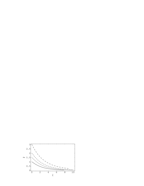
FIG. 7.: Time decay of the rotational perturbations $\hat{f}$ as a function of the string frame cosmological time in the case of non-vanishing potential dilaton field for different values of the parameter $\kappa$: $\kappa=1$ (solid curve), $\kappa=3/2$ (dotted curve), $\kappa=2$ (short dashed curve) and $\kappa=3$ (long dashed curve). We have used the normalization $\frac{\sqrt{C}}{2U_{0}^{3/2}}=1$.

FIG. 8.: String frame evolution of the deceleration parameter $\hat{q}$ for different values of the string coupling constant $\kappa$: $\kappa=1$ (solid curve), $\kappa=3/2$ (dotted curve), $\kappa=2$ (short dashed curve) and $\kappa=3$ (long dashed curve). We have used the normalization $\frac{\sqrt{C}}{2U_{0}^{3/2}}=1$.

V Discussions and Final Remarks

In this paper we have analyzed rotational perturbations of homogeneous flat isotropic FRW in NS-NS string cosmology. To first order in the metric rotation function the field equations reduce to the unperturbed field equations in addition to two equations determining the rotation function $\Omega(t,r)$. The decay of the rotation is basically determined by the dilaton field potential. The field equations impose strong constraint upon the functional form of $U(\phi)$, and except the trivial form $U(\phi)=0$ only one other form is allowed by the mathematical structure of the theory. In the Einstein frame the rotation function can be generally represented as a product of two independent functions, one depending on time and the other on $r$, plus a function depending on the cosmological time only.

If the dilaton field potential is zero, the large-time evolution of the rotational perturbations is determined by an arbitrary function of time $G(t)$ in both Einstein and string frames. Therefore in this case the initial rotation of the Universe may not decay to zero in the large time limit and thus the possibility of a global rotation in the present day Universe is not excluded in this model. On the other hand the arbitrary character of the function $G(t)$ and the absence of a physical mechanism excluding in a natural way rapid late-time rotation of the Universe raises the question if a dilaton potential free pre-big bang type cosmological model can lead to a correct description of the dynamics of our Universe. This situation is somehow similar to the behaviour of the anisotropy in the Bianchi type I space-times in pre-big bang cosmological models. In the absence of the dilaton field potential a Bianchi type I space-time does not isotropize, the geometry being of Kasner type for all times [17, 18]. Therefore in standard pre-big bang cosmological models with pure dilaton and axion fields nor the initial rotation neither the initial anisotropies can be washed out as a result of the expansionary evolution of the Universe.

For a non-zero dilaton potential the rotation Eq. (20) and the field equations completely determine the form of the potential. Therefore $U(\phi)$ is not an arbitrary parameter of the theory. In the Einstein frame the dilaton field potential, can be represented, as a function of time, in a parametric form, with $a$ taken as parameter, as

$$t-t_{0}=\int\frac{a^{2}da}{\sqrt{K+U_{0}^{2}a^{4}/4}},\qquad U(a)=U_{0}^{2}a^{-2}.$$ (59)

This mathematical form of the potential is the only one allowed by the mathematical structure of the field equations. In the limit of small $a$, $a\to 0$, the time dependence of the potential is given by $U(t)=U_{0}^{2}(3\sqrt{K}\,t)^{-2/3}$. In the limit of large $t$, corresponding to large $a$, we obtain $U(t)=4/t^{2}$. The behaviour of the dilaton field $\phi$ is described, as a function of the parameter $a$, by the equation

$$2\kappa a^{2}\left(K+\frac{U_{0}^{2}}{4}a^{4}\right)\left(\frac{d\phi}{da}\right)^{2}+C^{2}e^{-4\phi}-U_{0}^{2}a^{4}=2\kappa\phi_{0},$$ (60)

which follows from Eq. (16). The potential cannot be expressed as a function of the dilaton field in terms of elementary functions. In the small-time limit $a\to 0$ the dilaton field obeys the equation

$$2\kappa Ka^{2}\left(\frac{d\phi}{da}\right)^{2}=2\kappa\phi_{0}-C^{2}e^{-4\phi},$$ (61)

with the general solution

$$e^{2\phi}=\sqrt{\frac{C^{2}}{8\kappa\phi_{0}}}\left(a^{2\sqrt{\phi_{0}/K}}+a^{-2\sqrt{\phi_{0}/K}}\right)\approx\sqrt{\frac{C^{2}}{8\kappa\phi_{0}}}a^{-2\sqrt{\phi_{0}/K}}.$$ (62)

Therefore in the small-time limit the time dependence of the conformal transformation factor in the Einstein frame is

$$e^{2\phi}\approx\sqrt{\frac{C^{2}}{8\kappa\phi_{0}}}\left(3\sqrt{K}\,t\right)^{-\frac{2}{3}\sqrt{\phi_{0}/K}},$$ (63)

leading to a potential-dilaton field dependence of the exponential form

$$U(\phi)\approx U_{0}^{2}\left(\frac{8\kappa\phi_{0}}{C^{2}}\right)^{\frac{1}{2}\sqrt{K/\phi_{0}}}e^{2\sqrt{K/\phi_{0}}\,\phi}=\Lambda e^{2\chi\phi},$$ (64)

where $\Lambda=U_{0}^{2}\left(\frac{8\kappa\phi_{0}}{C^{2}}\right)^{\frac{1}{2}\sqrt{K/\phi_{0}}}=\hbox{const.}$ and $\chi=\sqrt{K/\phi_{0}}=\hbox{const.}$. The exponential type potentials play an important role in particle physics and cosmology. An exponential potential arises in the four-dimensional effective Kaluza-Klein theories from compactification of the higher-dimensional supergravity or superstring theories. In string or Kaluza-Klein theories the moduli fields associated with the geometry of the extra-dimensions may have effective exponential potentials due to the curvature of the internal spaces or to the interaction of the modului with form fields on the internal spaces. Exponential potentials can also arise due to the non-perturbative effects such as gaugino condensation (for a discussion on the role of exponential potentials in cosmology see [17] and references therein). In the large time limit the potential is a generalized exponential one, of the form $U(\phi)=g(\phi)e^{2\phi}$. The function $g(\phi)$ cannot be expressed in terms of elementary functions. In the string frame and in the same limit the dilaton field potential can be represented as $\hat{U}(\phi)=e^{2\phi}U(\phi)=4e^{2\phi}/t^{2}$. In the presence of the dilaton field potential there is a rapid decay of the rotational perturbations. The rotation equation (20) fixes not only the form of the potential but also determines the mathematical form of the function $G(t)$, which in the Einstein frame is inversely proportional to the third power of the scale factor. Hence in an expanding Universe the rotational perturbations decrease rapidly, the long-time decay of the rotation being given by a power law in the Einstein and by an exponential term in the string frame. The general physical requirement of the very small (or zero) rotation of the late-time Universe also imposes the presence of the axion field, together with the dilaton field potential, in the very early stages of cosmological evolution.

If the Kalb-Ramond field $h$ is zero, even in the presence of the dilaton field potential, the rotational perturbations in the string frame are governed by the numerical value of the string coupling constant $\kappa$. In this case the Universe is not rotating for large cosmological times only if $\kappa>2$. For string theory $\kappa=2$ and for a zero $h$-field the corresponding dilatonic Universe rotates for all times.

The observational evidence that our Universe is rotating very slowly or at all imposes a major constraint on realistic cosmological models. The first order rotational perturbation theory analyzed in the present paper could be relevant for the understanding of the transient period from a rotating initial state of our Universe to an expansionary one.

REFERENCES

- [1] G. Gamow, Rotating universe?, Nature 158 (1946) 549.
- [2] P. Birch, Is the universe rotating?, Nature 298 (1982) 451-454.
- [3] P. Birch, Is there evidence for universal rotation? Birch replies, Nature 301 (1982) 736.
- [4] B. Nodland and J. P. Ralston, Indication of anisotropy in electromagnetic propagation over cosmological distances, Phys. Rev. Lett. 78 (1997) 3043-3046; astro-ph/9704196.
- [5] R. W. Kühne, On the cosmic rotation axis, Mod. Phys. Lett. A12 (1997) 2473-2474; astro-ph/9708109.
- [6] C. B. Collins and S. W. Hawking, The rotation and distortion of the universe, Mon. Not. R. astr. Soc. 162 (1973) 307-320.
- [7] J. D. Barrow, R. Juszkiewicz and D. H. Sonoda, Universal rotation: how large can it be, Mon. Not. R. astr. Soc. 213 (1985) 917-943.
- [8] K. Gödel, An example of a new type of cosmological solutions of Einstein’s field equations for gravitation, Rev. Mod. Phys. 21 (1949) 447-450.
- [9] Yu. N. Obukhov, On physical foundations and observational effects of cosmic rotation, in: Colloquium on Cosmic Rotation, eds. M. Scherfner, T. Chrobok and M. Shefaat, Wissenschaft und Technik Verlag, Berlin (2000) 23-96; astro-ph/0008106.
- [10] J. Ellis and K. A. Olive, Inflation can solve the rotation problem, Nature 303 (1983) 679-681.
- [11] Ø. Grøn and H. H. Soleng, Decay of primordial cosmic rotation in inflationary cosmologies, Nature 328 (1987) 501-503.
- [12] M. Gasperini and G. Veneziano, Pre-big bang in string cosmology, Astropart. Phys. 1 (1993) 317-339; hep-th/9211021.
- [13] E. Di Pietro and J. Demaret, Scale factor duality in string Bianchi cosmologies, Int. J. Mod. Phys. D8 (1999) 349-361; gr-qc/9903063.
- [14] J. E. Lidsey, D. Wands and E. J. Copeland, Superstring cosmology, hep-th/9909061.
- [15] J. D. Barrow and M. P. Dabrowski, Gödel universe in string theory, Phys. Rev. D58 (1998) 103502; gr-qc/9803048.
- [16] V. F. Mukhanov, F. A. Feldman and R. H. Brandenberger, Theory of cosmological perturbations. Part 1. Classical perturbations. Part 2. Quantum theory of perturbations. Part 3. Extensions, Phys. Rep. 215 (1992) 203-333.
- [17] C.-M. Chen, T. Harko and M. K. Mak, Bianchi type I cosmologies in arbitrary dimensional dilaton gravities, Phys. Rev. D 62 (2000) 124016; hep-th/0004096.
- [18] C.-M. Chen, T. Harko and M. K. Mak, Anisotropic four-dimensional Neveu-Schwarz–Neveu-Schwarz string cosmology, to appear in Phys. Rev. D; hep-th/0005236.