UG/00-18

SU-ITP-00/31

KUL-TF-00/29

hep-th/0012110

Supersymmetry of RS bulk and brane ^†
Eric Bergshoeff ¹, Renata Kallosh,², and Antoine Van Proeyen ³

¹ Institute for Theoretical Physics, Nijenborgh 4, 9747 AG Groningen, The Netherlands
² Department of Physics, Stanford University, Stanford, CA 94305, USA
³ Instituut voor Theoretische Fysica, Katholieke Universiteit Leuven,
Celestijnenlaan 200D B-3001 Leuven, Belgium

Abstract

We review the construction of actions with supersymmetry on spaces with a domain wall. The latter objects act as sources inducing a jump in the gauge coupling constant. Despite these singularities, supersymmetry can be formulated, maintaining its role as a square root of translations in this singular space. The setup is designed for the application in five dimensions related to the Randall–Sundrum (RS) scenario. The space has two domain walls. We discuss the solutions of the theory with fixed scalars and full preserved supersymmetry, in which case one of the branes can be pushed to infinity, and solutions where half of the supersymmetries are preserved.   To be published in the proceedings of the NATO advanced research workshop Noncommutative structures in mathematics and physics in Kiev and in the proceedings of the EC-RTN workshop The quantum structure of spacetime and the geometric nature of fundamental interactions in Berlin. Talks given by A.V.P.

1 Introduction

It is not obvious how supersymmetry can be implemented in a space with domain walls. The wall is at a fixed place and its presence seems to lead to a breaking of translations orthogonal to the plane. Supersymmetry, being the square root of translations, seems rather difficult to realize in this context. It is interesting to see how this obstacle has been avoided in [1], which we summarize here.

The work is mostly motivated by the Randall–Sundrum (RS) scenarios [2]. The simplest form of the situation that is under investigation consists of a 3-brane in a 5-dimensional bulk. The solution can be generalized e.g. to 8-branes in $D=10$, but the full implementation of that situation is still under investigation.

When the RS scenarios appeared, supersymmetrisation was soon investigated. After initial attempts, it was found that no smooth supersymmetric RS single-brane scenario is possible [3]. This scenario with one brane was put forward as an alternative to compactification.

This lead us to the original RS setup with two branes. The 2-brane scenario has a compactified fifth dimension, $x_{5}\simeq x_{5}+2\tilde{x}_{5}$, with two branes fixed at $x_{5}=0$ and $x_{5}=\tilde{x}_{5}$.

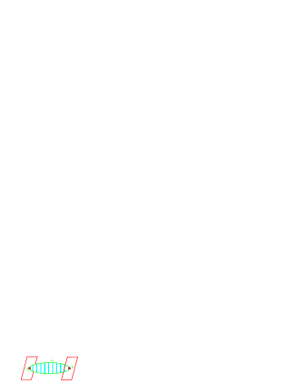
Figure 1: Two-brane scenario. The fifth dimension is a circle with branes at opposite ends and a $\mathbb{Z}_{2}$ identification of points symmetric w.r.t. $x_{5}=0$.

There is moreover an orbifold condition relating points $x_{5}$ and $-x_{5}$. Thus, the five-dimensional manifold has the form ${\bf M}={\bf M}_{4}\times{S^{1}\over\mathbb{Z}_{2}}$. This is similar to the Hořava–Witten [4] scenario. The latter one embeds 10-dimensional manifolds in an 11-dimensional space. They obtain the supersymmetry by a cancellation between anomalies of the bulk theory and a non-invariance of the classical brane action. Lukas, Ovrut, Stelle and Waldram [5] reduced this on a Calabi–Yau manifold to five dimensions, and further developed this setup in five dimensions. Further steps have been taken by [6, 7, 8, 9]. In [7, 9] the gauge coupling constant does not change when crossing the branes, while in [6, 8] this coupling constant changes sign. In that respect, our approach is most close to the latter. In these papers, the action in the bulk is modified, such that it is not supersymmetric any more by itself, but the non-invariance is compensated by the brane action to obtain invariance of the total action. We [1] obtain separate invariance of bulk and brane action.

The first part of this report will treat the construction of the action with local supersymmetry on the singular space. In that part, we will show how the bulk and brane action are separately invariant under supersymmetry. The supersymmetry that we are considering is the one with 8 real components, i.e. minimal (${\cal N}=2$) supersymmetry in 5 dimensions. The algebra is preserved despite the discontinuity. The second part treats background solutions. The Killing spinors are discussed. There are solutions with fixed scalars and 8 Killing spinors, and solutions of $1/2$ supersymmetry, i.e. with 4 Killing spinors. Finally a summary is given, discussing open issues.

2 The action for bulk and brane

The construction of the action involves three steps. First, we consider the bulk action. That is the action of supergravity in $D=5$ with matter couplings. A quite general action has been given in [10] based on the general methods developed in 4 dimensions in [11]. But it may not be excluded that further generalizations are possible [12]. We will restrict ourselves to the couplings of vector multiplets, for which the general couplings were found in [13]. One can separate the ungauged part, and the part dependent on a gauge coupling constant $g$. We will consider only the gauging of a $\mathop{\rm{}U}(1)$ $R$-symmetry group.

In the second step, the gauge coupling constant $g$ is replaced by a field $G(x)$. A Lagrange multiplier field, a $(D-1)$-form (4-form for our application), is introduced, whose field equation imposes the constancy of $G(x)$ such that effectively it is still a constant.

The third step introduces the brane action. That action has extra terms for the Lagrange multiplier $(D-1)$-form, which allows $G(x)$ to vary crossing the brane. We will show how every step preserves the supersymmetry!

Before embarking on that programme, we want to repeat the fundamental algebraic relation between the cosmological constant and the gauge coupling constant of $R$-symmetry. The super-anti-de Sitter algebra for ${\cal N}=2$ in $D=5$ is $\mathop{\rm SU}(2,2|1)$. It involves the anti-de Sitter algebra $\mathop{\rm SO}(4,2)\simeq\mathop{\rm SU}(2,2)$ with translations $P_{a}$ and Lorentz rotations $M_{ab}$, the supersymmetries $Q^{i}$, with $i=1,2$, a symplectic Majorana spinor, and a $\mathop{\rm{}U}(1)$ generator as $R$-symmetry. The most characteristic (anti)commutator relations are

$$\left\{Q^{i},Q^{j}\right\} = {\textstyle\frac{1}{2}}\varepsilon^{ij}\gamma_{a}P^{a}+{\rm i}gQ^{ij}\gamma^{ab}M_{ab}+{\rm i}\varepsilon^{ij}U\,,$$

$$\left[U,Q^{i}\right] = gQ^{i}{}_{j}\,Q^{j}\,,$$

$$\left[P_{a},P_{b}\right] = g^{2}Q^{i}{}_{j}Q^{j}{}_{i}\,M_{ab}\,,$$

$$\left[P_{a},Q^{i}\right] = {\rm i}\gamma_{a}gQ^{i}{}_{j}Q^{j}\,.$$ (2.1)

$Q_{ij}$ satisfies

$$Q_{ij}=Q_{ji}\,,\qquad Q^{i}{}_{j}\equiv\varepsilon^{ik}Q_{kj}={\rm i}\left(q_{1}\sigma_{1}+q_{2}\sigma_{2}+q_{3}\sigma_{3}\right)\,,$$

$$q_{1},\,q_{2}\,,q_{3}\in\mathbb{R}\,,\qquad(q_{1})^{2}+(q_{2})^{2}+(q_{3})^{2}=1\,.$$ (2.2)

This matrix determines the embedding of $\mathop{\rm{}U}(1)$ in the automorphism group of the supersymmetries $\mathop{\rm SU}(2)$. This choice is not physically relevant in itself. The second of the commutators in (2.1) implies that $g$ is the coupling constant of $R$-symmetry. But the third equation says that $g^{2}$ determines the curvature of spacetime, i.e. it determines the cosmological constant. This fact is the cornerstone of the situation that we describe. The gauge coupling and the cosmological constant are related. However, one can change the coupling constant from $+g$ to $-g$, not affecting the cosmological constant. That is what will happen going through the branes. This jump in the sign of $g$ will thus occur together with the action of the $\mathbb{Z}_{2}$. This $\mathbb{Z}_{2}$ acts on the fields, which therefore live on an orbifold. One can distinguish odd and even fields. The circle condition on the fields and the orbifold condition are then

$$\Phi(x^{5})=\Phi(x^{5}+2\tilde{x}^{5})\,,$$

$$\Phi_{\rm even}(-x^{5})=\Phi_{\rm even}(x^{5})\,,\qquad\Phi_{\rm odd}(-x^{5})=-\Phi_{\rm odd}(x^{5})\,.$$ (2.3)

These conditions imply that odd fields vanish on the branes: at $x^{5}=0$ and at $x^{5}=\tilde{x}^{5}$.

Also the supersymmetries split. Half of them are even, and half are odd. Therefore, on the brane one has 4 supersymmetries, i.e. ${\cal N}=1$ in 4 dimensions. This splitting of the fermions requires a projection matrix in $\mathop{\rm SU}(2)$ space. Now the relative choice of this projection matrix and $Q$ in (2.2) matters. If they anticommute, the choice that has been taken in [7, 9], then $g$ does not change when one crosses the brane. If they commute, as in [6, 8], then $g$ jumps over the brane. And the latter is what we will take further.

After these general remarks, we come to step 1. We thus consider the action of supergravity coupled to $n$ vector multiplets [13]. The fields are

$$e_{\mu}^{a}\,,\ \psi_{\mu}^{i}\,,\ A_{\mu}^{I}\,,\ \varphi^{x}\,,\ \lambda^{ix}\,,$$ (2.4)

i.e. the graviton, gravitini, $n+1$ gauge fields ($I=0,1,\ldots,n$), including the graviphoton, $n$ scalars ($x=1,\ldots,n$), and $n$ doublets of spinors. The scalars describe a manifold structure that has been called very special geometry [14]. That geometry, and the complete action, is determined by a symmetric tensor $C_{IJK}$. The scalars are best described as living in an $n$-dimensional scalar manifold embedded in an $(n+1)$-dimensional space. $h^{I}$ are the coordinates of this larger space. The submanifold is defined by an embedding condition such that the $h^{I}$ as functions of the independent coordinates $\varphi^{x}$ should satisfy

$$h^{I}(\varphi)h^{J}(\varphi)h^{K}(\varphi)C_{IJK}=1\,.$$ (2.5)

The metric and all relevant quantities of this bulk theory is thus so far only dependent on $C_{IJK}$.

Then we add the gauging of a $\mathop{\rm{}U}(1)$ group. That means that we take a linear combination of the vectors as gauge field for this $R$-symmetry. The linear combination is defined by real constants $V_{I}$:

$$A_{\mu}^{(R)}\equiv V_{I}A_{\mu}^{I}\,.$$ (2.6)

The action and the transformation laws are then modified by terms that all depend on $gQ^{i}{}_{j}$.

In step 2, the coupling constant $g$ is replaced by a coupling field $G(x)$. In the Günaydin–Sierra–Townsend (GST) action, the coupling constant appears up to terms in $g^{2}$. We thus replace

$$S_{GST}(g)=S_{0}+gS_{1}+g^{2}S_{2}\ \Rightarrow\ S_{GST}(G(x))=S_{0}+G(x)S_{1}+G(x)^{2}S_{2}\,.$$ (2.7)

Another term is added to the bulk action that forces $G(x)$ to be a constant, using a Lagrange-multiplier 4-form $A_{\mu\nu\rho\sigma}$:

$$S_{\rm bulk} = S_{GST}(G(x))+\int{\rm d}^{5}x\,e\,\frac{1}{4!}\varepsilon^{\mu\nu\rho\sigma\tau}A_{\mu\nu\rho\sigma}\partial_{\tau}G(x)$$ (2.8)

$$= S_{0}-\int{\rm d}^{5}x\,e\,V-\int{\rm d}^{5}x\,e\,\hat{F}(x)G(x)+\mbox{fermionic terms.}$$

In the second line, the terms have been reordered. The potential $V$ originates from $S_{2}$ in (2.7), and leads to the potential

$$V=-6G^{2}\left[W^{2}-\frac{3}{4}\left({\partial W\over\partial\varphi^{x}}\right)^{2}\right]\,,\qquad W\equiv\sqrt{{\textstyle\frac{2}{3}}}h^{I}V_{I}\,,$$ (2.9)

where the linear combination $W$ appears, analogous to (2.6). The third term in (2.8) appears from integrating by part the term with the Lagrange multiplier, leading to the flux

$$\hat{F}\equiv{\textstyle\frac{1}{4!}}e^{-1}\varepsilon^{\mu\nu\rho\sigma\tau}\partial_{\mu}A_{\nu\rho\sigma\tau}+\mbox{covariantization.}$$ (2.10)

The covariantization terms come from $S_{1}$ in (2.7). This method of describing a constant using a $(D-1)$-form is in fact an old method that was already used in [15].

It is easy to understand how supersymmetry is preserved. Indeed, the GST action is known to be invariant:

$$\delta(\epsilon)S_{GST}(g)=0\,.$$ (2.11)

Therefore, the only non-invariance for $S_{GST}(G(x))$ appears, if we define $\delta(\epsilon)G=0$, from the $x$-dependence of $G(x)$. It is thus proportional to its spacetime derivative

$$\delta(\epsilon)S_{GST}(G(x))=B^{\mu}\,\partial_{\mu}G(x)\,,$$ (2.12)

where $B^{\mu}$ is some expression of the other fields and parameters, whose exact form is not important for the argument here. One immediately sees then that invariance of (2.8) is obtained by defining the transformation law of the 4-form as

$$\delta(\epsilon)\frac{1}{4!}\varepsilon^{\mu\nu\rho\sigma\tau}A_{\mu\nu\rho\sigma}=B^{\tau}=e\left[-{\rm i}{\textstyle\frac{3}{2}}\overline{\psi}{}_{\mu}^{i}\gamma^{\mu\tau}\epsilon^{j}W-\overline{\psi}{}_{\mu}^{i}\gamma^{\mu\tau\rho}\epsilon^{j}A^{(R)}_{\rho}+{\textstyle\frac{3}{2}}\overline{\lambda}{}^{i}_{x}W^{,x}\gamma^{\tau}\epsilon^{j}\right]Q_{ij}\,,$$ (2.13)

where we gave also the explicit form for our case. However, it is clear that the method is also valid in other theories.

Step 3 introduces the brane action, such that the total action is

$$S_{\rm new}=S_{\rm bulk}+S_{\rm brane}\,.$$ (2.14)

The brane action has the form

$$S_{\rm brane} = -2g\int{\rm d}^{5}x\,\left(\delta(x^{5})-\delta(x^{5}-\tilde{x}^{5})\right)\left(e_{(4)}3W+{\textstyle\frac{1}{4!}}\varepsilon^{{\underline{\mu}}{\underline{\nu}}{\underline{\rho}}{\underline{\sigma}}}A_{{\underline{\mu}}{\underline{\nu}}{\underline{\rho}}{\underline{\sigma}}}\right)$$ (2.15)

$$= S_{brane,1}-S_{brane,2}\,.$$

Underlined indices refer to the values in the brane directions: $\underline{\mu}=0,1,2,3$. The action is presented as an integral over 5 dimensions, but the delta functions imply that it is a four-dimensional action for each brane separately. The action of each brane consists of a Dirac–Born–Infeld (DBI) term and a Wess–Zumino (WZ) term. However, both parts depend only on the pullback of the bulk fields to the branes. There are no fields living on the brane. The function $W$ appears in the DBI term, and plays the role of the central charge of the brane. But most importantly, the 4-form Lagrange multiplier appears in the WZ term, and this thus modifies its field equation. The new field equation is

$$\partial_{5}G(x^{5})=2g\left(\delta(x^{5})-\delta(x^{5}-\tilde{x}^{5})\right)\,,$$ (2.16)

and leads to the solution (taking into account the cyclicity condition)

$$G(x)=g\,\varepsilon(x^{5})\,.$$ (2.17)

The function $\varepsilon(x^{5})$ jumps as well at $x^{5}=0$ as at $x^{5}=\tilde{x}^{5}$, see figure 2.

Figure 2: The coupling constant $g$ jumps at $x_{5}=0$ and at $x_{5}=\tilde{x}_{5}$.

It is clear from this picture that we need the second brane. Indeed, one has to come back to the original value of $g$, in order that total derivatives in $x^{5}$ do not contribute to the action. The flux, which is determined by the field equation of $G(x)$, is

$$\hat{F}=12G\left[W^{2}-\frac{3}{4}\left({\partial W\over\partial\varphi^{x}}\right)^{2}\right]+\mbox{fermionic terms.}$$ (2.18)

The overall factor changes when crossing each brane due to (2.17). These jumps imply that the wall acts as a sink for the fluxes.

That supersymmetry is still preserved by the addition of the brane is less obvious and is the non-trivial part of the construction. It turns out that the supersymmetry is preserved thanks to the projections. One finds (indices $m$ are tangent space indices in brane directions)

$$\delta S_{\rm brane} =-3g\int d^{5}x\left(\delta(x^{5})-\delta(x^{5}-\tilde{x}^{5})\right)e_{(4)} \left[W\bar{\epsilon}^{i}\gamma^{m}e_{m}^{\underline{\mu}}\left(\psi_{{\underline{\mu}}i}-{\rm i}\gamma_{5}Q_{ij}\psi_{\underline{\mu}}^{j}\right)+\right.$$ (2.19)

$$\left.\ \ +\,W_{,x}\bar{\epsilon}^{i}\left({\rm i}\lambda_{i}^{x}-\gamma_{5}Q_{ij}\lambda^{xj}\right)\right].$$

The combinations of the gravitino and the gauginos that are in brackets are the components that are odd under the $\mathbb{Z}_{2}$ projection, and thus vanish on the brane. This leads to the invariance. Remark that in each case one of the two terms comes from the DBI (mass) term and the other from the WZ (charge) term. This therefore determines the relative weight of the two terms, and is the mass $=$ charge relation, that says that the brane is BPS. We thus see, indeed, that the brane action is separately invariant. Note, that if we would not use (or eliminate) the Lagrange multiplier, then this would relate bulk and brane, and only the sum would be invariant.

3 The background: BPS solutions

We consider solutions with a warped metric, i.e.

$${\rm d}s^{2}=a^{2}(x^{5})\,{\rm d}x^{\underline{\mu}}{\rm d}x^{\underline{\nu}}\eta_{{\underline{\mu}}{\underline{\nu}}}+({\rm d}x^{5})^{2}\,.$$ (3.1)

The energy density for solutions that depend only on $x^{5}$ is

$$E(x^{5}) = -6a^{2}a^{\prime 2}+{\textstyle\frac{1}{2}}a^{4}(\varphi^{x\prime})^{2}+a^{4}V-{\textstyle\frac{1}{4!}}\varepsilon^{\mu\nu\rho\sigma 5}A_{\mu\nu\rho\sigma}G^{\prime}+$$ (3.2)

$$+\,2g\left(\delta(x^{5})-\delta(x^{5}-\tilde{x}^{5})\right)\left(3a^{4}W+{\textstyle\frac{1}{4!}}\varepsilon^{{\underline{\mu}}{\underline{\nu}}{\underline{\rho}}{\underline{\sigma}}}A_{{\underline{\mu}}{\underline{\nu}}{\underline{\rho}}{\underline{\sigma}}}\right),$$

where the prime denotes a derivative w.r.t. $x^{5}$. The first three terms come from the GST action, the last one on the first line from the term that we added with the Lagrange multiplier. The second line comes from the brane action. For this type of brane actions, one can rewrite it using squares and total derivatives:

$$E = \frac{1}{2}a^{4}\left\{\left[\varphi^{x\prime}-3GW^{,x}\right]^{2}-12[{a^{\prime}\over a}+GW]^{2}\right\}+3[a^{4}GW]^{\prime}+$$ (3.3)

$$+\,\left[2g\left(\delta(x^{5})-\delta(x^{5}-\tilde{x}^{5})\right)-G^{\prime}\right]\left(3a^{4}W+{\textstyle\frac{1}{4!}}\varepsilon^{{\underline{\mu}}{\underline{\nu}}{\underline{\rho}}{\underline{\sigma}}}A_{{\underline{\mu}}{\underline{\nu}}{\underline{\rho}}{\underline{\sigma}}}\right).$$

The expression in square brackets in the second line is the field equation of the Lagrange multiplier, and this line can thus be omitted. The last term of the first line is a total derivative in $x^{5}$ and thus also does not contribute to the energy due to the continuity of the fields. The vanishing of the squared terms gives thus the minimum of the energy, and this minimum is even zero, as the zero energy of a closed universe. The BPS conditions are thus

$$\varphi^{x\prime}=3G\,W^{,x}\,,\qquad{a^{\prime}\over a}=-G\,W\,.$$ (3.4)

These equations are also called stabilization equations. These equations are important to investigate the preserved supersymmetries. The transformations of the fermions are

$$\delta(\epsilon)\lambda_{i}^{x} = -{\rm i}{\textstyle\frac{1}{2}}\gamma_{5}\varphi^{x\prime}\epsilon_{i}-{\textstyle\frac{3}{2}}GQ_{ij}W^{,x}\epsilon^{j}\,,$$

$$\delta(\epsilon)\psi_{{\underline{\mu}}i} = \partial_{\underline{\mu}}\epsilon_{i}+{\textstyle\frac{1}{2}}\delta_{\underline{\mu}}^{m}\gamma_{m}\left(a^{\prime}\gamma_{5}\epsilon_{i}+{\rm i}aGQ_{ij}W\epsilon^{j}\right)\,,$$

$$\delta(\epsilon)\psi_{5i} = \epsilon^{\prime}_{i}+{\textstyle\frac{1}{2}}{\rm i}GQ_{ij}W\gamma_{5}\epsilon^{j}\,.$$ (3.5)

To solve these, we split the supersymmetries in their even and odd parts:

$$\epsilon_{i}=\epsilon_{i}^{+}+\epsilon_{i}^{-}\,,\qquad\epsilon_{i}^{\pm}={\textstyle\frac{1}{2}}\left(\epsilon_{i}\pm{\rm i}\gamma_{5}Q_{ij}\epsilon^{j}\right)=\pm{\rm i}\gamma_{5}Q_{ij}\epsilon^{\pm j}\,.$$ (3.6)

The vanishing of the last transformation of (3.5) determines the $x^{5}$ dependence of both parts. We have $\epsilon_{i}^{\pm}=a^{\pm 1/2}\epsilon_{i}^{\pm}(x^{\underline{\mu}})$. The transformations of the other components of the gravitino then determines the dependence on the other four spacetime variables. This gives the general solution,

$$\epsilon_{i}=a^{1/2}\epsilon_{i}^{+(0)}+a^{-1/2}\left(1-\frac{a^{\prime}}{a}x^{\underline{\mu}}\gamma_{\underline{\mu}}\gamma_{5}\right)\epsilon_{i}^{-(0)}\,,$$ (3.7)

as function of $\epsilon_{i}^{\pm(0)}$, which are constant spinors with each only 4 real components. There remains the transformations of the gaugino, which lead to

$$\varphi^{x\prime}\epsilon_{i}^{-(0)}=0\,.$$ (3.8)

This leaves two possibilities. The first factor can be zero, which implies that we have constant scalars. In that case 8 Killing spinors survive. The other possibility allows non-constant scalars. Then the second factor should be zero, and this thus eliminates 4 supersymmetries. There remain 4 Killing spinors, $\epsilon_{i}^{+(0)}$, which are the 4 that are non-vanishing also on the brane.

We consider both possibilities. First, let us look at the situation with fixed scalars. The BPS equations are then

$$(\varphi^{y})^{\prime}=0\,,\qquad\left({\partial W\over\partial\varphi^{x}}\right)_{\rm crit}=0\,,\qquad\frac{a^{\prime}}{a}=-g\varepsilon(x^{5})W\,.$$ (3.9)

The constancy of $W$ is translated by formulae of very special geometry in a ‘supersymmetric attractor equation’

$$C_{IJK}\bar{h}^{J}\bar{h}^{K}=q_{I}\,,\qquad\bar{h}^{K}\equiv\sqrt{W_{crit}}h^{K}\,,\qquad q_{I}\equiv\sqrt{{\textstyle\frac{2}{3}}}V_{I}\,.$$ (3.10)

This equation is well-known from black-hole physics [16]. A solution gives rise to a metric of the form

$${\rm d}s^{2}=e^{-2gW_{\rm crit}|x^{5}|}{\rm d}x^{\underline{\mu}}{\rm d}x^{\underline{\nu}}\eta_{{\underline{\mu}}{\underline{\nu}}}+({\rm d}x^{5})^{2}\,,\qquad\mbox{or}\qquad a=e^{-2gW_{crit}|x^{5}|}\,.$$ (3.11)

In this case, the negative-tension brane can be pushed to infinity. Indeed, there is no obstruction as $a$ never vanishes.

To consider supersymmetric domain walls with non-constant scalars, we use another coordinate, $y$, such that ${\partial\over\partial x^{5}}=a^{2}{\partial\over\partial y}$. The metric is then

$${\rm d}s^{2}=a^{2}(y){\rm d}x^{\underline{\mu}}{\rm d}x^{\underline{\nu}}\eta_{{\underline{\mu}}{\underline{\nu}}}+a^{-4}(y){\rm d}y^{2}\,.$$ (3.12)

The stabilization equations take the form

$$a^{2}\frac{{\rm d}}{{\rm d}y}{\varphi^{x}}=3G(y)W^{,x}\,,\qquad a\frac{{\rm d}}{{\rm d}y}a=-G(y)\,W\,.$$ (3.13)

These $n+1$ equations are combined, using relations of very special geometry, to

$${{\rm d}\over{\rm d}y}(C_{IJK}\tilde{h}^{J}\tilde{h}^{K})=-2G(y)q_{I}\qquad\mbox{where}\qquad\tilde{h}^{I}\equiv a(y)h^{I}\,,$$ (3.14)

whose solutions are given in terms of harmonic functions $H_{I}(y)$:

$$C_{IJK}\tilde{h}^{J}\tilde{h}^{K}=H_{I}(y)=c_{I}-2gq_{I}|y|\,,$$ (3.15)

where $c_{I}$ are integration constants, while $q_{I}$ are the constants that were introduced in the gauging ($V_{I}$ up to a normalization). They are harmonic in the sense that

$${{\rm d}\over{\rm d}y}{{\rm d}\over{\rm d}y}H_{I}=-4gq_{I}[\delta(y)-\delta(y-\tilde{y})]\,.$$ (3.16)

The warp factor is

$$a^{2}(y)=h^{I}H_{I}\,.$$ (3.17)

In this case the distance between the branes is restricted. There can be two types of restrictions:

1. There can be fundamental restrictions due to the origin of the functions $h^{I}$. E.g. these are in various applications related to integrals over Calabi–Yau cycles. Their vanishing can put a restriction on the distance.

2. The vanishing of the harmonic functions also puts a restriction. Indeed, these harmonic functions enter in the warp factor, which should be non-vanishing.

In each case this restricts the distance to be smaller than a critical distance

$$|\tilde{y}|<|y|_{\rm sing}\,.$$ (3.18)

4 Summary and outlook

The RS scenario in 5 dimensions can be made supersymmetric despite the singularities of the space. The action and transformation laws can be obtained using a 4-form, such that bulk and brane are separately supersymmetric. Supersymmetric solutions exist with fixed scalars or 1/2 supersymmetry.

Half of the supersymmetries vanish on the branes. Also the translation generator in the fifth direction vanishes on the brane. That is how the algebra can be realized. These algebraic aspects could still be clarified further. Also the extension to hypermultiplets deserves further study. The same mechanism could be applied to study 8-branes in $D=10$ and other similar situations. It is furthermore an intriguing question how supersymmetric matter can live on the branes.

References

- [1] E. Bergshoeff, R. Kallosh and A. Van Proeyen, Supersymmetry in singular spaces, JHEP 10 (2000) 033 [hep-th/0007044].
- [2] L. Randall and R. Sundrum, A large mass hierarchy from a small extra dimension, Phys. Rev. Lett. 83, 3370 (1999) [hep-ph/9905221]; An alternative to compactification, Phys. Rev. Lett. 83, 4690 (1999) [hep-th/9906064].
-
[3]
R. Kallosh and A. Linde, Supersymmetry and the brane world, JHEP
0002, 005 (2000) [hep-th/0001071];
K. Behrndt and M. Cvetič, Anti-de Sitter vacua of gauged supergravities with 8 supercharges, Phys. Rev. D61, 101901 (2000) [hep-th/0001159]. - [4] P. Hořava and E. Witten, Eleven-dimensional supergravity on a manifold with boundary, Nucl. Phys. B475 (1996) 94 [hep-th/9603142].
- [5] A. Lukas, B.A. Ovrut, K.S. Stelle and D. Waldram, The universe as a domain wall, Phys. Rev. D59 (1999) 086001 [hep-th/9803235]; Heterotic M-theory in five dimensions, Nucl. Phys. B552 (1999) 246 [hep-th/9806051].
- [6] T. Gherghetta and A. Pomarol, Bulk fields and supersymmetry in a slice of AdS, Nucl. Phys. B586 (2000) 141 [hep-ph/0003129].
- [7] R. Altendorfer, J. Bagger and D. Nemeschansky, Supersymmetric Randall–Sundrum scenario, hep-th/0003117.
- [8] A. Falkowski, Z. Lalak and S. Pokorski, Supersymmetrizing branes with bulk in five-dimensional supergravity, Phys. Lett. B491 (2000) 172 [hep-th/0004093].
- [9] M. Zucker, Supersymmetric brane world scenarios from off-shell supergravity, hep-th/0009083.
- [10] A. Ceresole and G. Dall’Agata, General matter coupled , gauged supergravity, Nucl. Phys. B585 (2000) 143 [hep-th/0004111].
- [11] L. Andrianopoli, M. Bertolini, A. Ceresole, R. D’Auria, S. Ferrara, P. Frè and T. Magri, supergravity and super Yang–Mills theory on general scalar manifolds: Symplectic covariance, gaugings and the momentum map, J. Geom. Phys. 23 (1997) 111 [hep-th/9605032].
- [12] K. Behrndt, C. Herrmann, J. Louis and S. Thomas, Domain walls in five dimensional supergravity with non-trivial hypermultiplets, hep-th/0008112.
-
[13]
M. Günaydin, G. Sierra and P.K. Townsend, The geometry of
Maxwell–Einstein supergravity and Jordan algebras, Nucl. Phys. B242 (1984) 244;
Gauging the Maxwell–Einstein supergravity theories: more on Jordan algebras, Nucl. Phys. B253 (1985) 573. - [14] B. de Wit and A. Van Proeyen, Broken sigma model isometries in very special geometry, Phys. Lett. B293 (1992) 94 [hep-th/9207091].
- [15] A. Aurilia, H. Nicolai and P.K. Townsend, Hidden constants: the theta parameter of QCD and the cosmological constant of supergravity, Nucl. Phys. B176 (1980) 509.
-
[16]
S. Ferrara, R. Kallosh and A. Strominger, extremal black
holes,
Phys. Rev. D52, 5412 (1995) [hep-th/9508072];
S. Ferrara and R. Kallosh, Supersymmetry and attractors, Phys. Rev. D54, 1514 (1996) [hep-th/9602136]; Universality of supersymmetric attractors, Phys. Rev. D54, 1525 (1996) [hep-th/9603090].