THE EXACT RENORMALIZATION GROUP AND FIRST-ORDER PHASE TRANSITIONS

Studies of first-order phase transitions through the use of the exact renormalization group are reviewed. In the first part the emphasis is on universal aspects: We discuss the universal critical behaviour near weakly first-order phase transitions for a three-dimensional model of two coupled scalar fields – the cubic anisotropy model. In the second part we review the application of the exact renormalization group to the calculation of bubble-nucleation rates. More specifically, we concentrate on the pre-exponential factor. We discuss the reliability of homogeneous nucleation theory that employs a saddle-point expansion around the critical bubble for the calculation of the nucleation rate.

1 Weakly first-order phase transitions

Weakly first-order phase transitions appear in many statistical systems (such as superconductors or anisotropic systems) and in high-temperature field theories. Many cosmological phase transitions, such as the electroweak $\!{}^{{\bf?}}$, fall in this category. However, a reliable quantitative description of these phenomena is still lacking.

A simple example of a system with an arbitrarily weakly first-order phase transition is the cubic anisotropy model $\!{}^{{\bf?},{\bf?}}$. In field-theoretical language, it corresponds to a theory of two real scalar fields $\phi_{a}~{}(a=1,2)$ in three dimensions, invariant under the discrete symmetry $(1\leftrightarrow-1,2\leftrightarrow-2,1\leftrightarrow 2)$. It can also be considered as the effective description of the four-dimensional high-temperature theory with the same symmetry, at energy scales smaller than the temperature $\!{}^{{\bf?}}$.

The properties of the weakly first-order phase transitions in this model have been studied within the $\epsilon$-expansion $\!{}^{{\bf?}}$ or through Monte Carlo simulations $\!{}^{{\bf?}}$. In particular, universal amplitudes have been computed, which describe the relative discontinuity of various physical quantities along the phase transition, in the limit when the transition becomes arbitrarily weakly first order. A discrepancy has been observed in the predictions for the universal ratio of susceptibilities $\chi_{+}/\chi_{-}$ on either side of the phase transition, obtained through Monte Carlo simulations or the $\epsilon$-expansion $\!{}^{{\bf?}}$. The Monte Carlo simulations predict $\chi_{+}/\chi_{-}=4.1(5)$, while the first three orders of the $\epsilon$-expansion give $\chi_{+}/\chi_{-}=2.0,2.9,2.3$ respectively.

We summarize here the results of an alternative approach $\!{}^{{\bf?}}$ that employs the exact renormalization group. It is based on the effective average action $\Gamma_{k}$ $\!{}^{{\bf?}}$, which is a coarse-grained free energy with an infrared cutoff. More precisely, $\Gamma_{k}$ incorporates the effects of all fluctuations with momenta $q^{2}>k^{2}$, but not those with $q^{2}<k^{2}$. In the limit $k\rightarrow 0$, the effective average action becomes the standard effective action (the generating functional of the 1PI Green functions), while at a high momentum scale (of the order of the ultraviolet cutoff) $k=\Lambda\rightarrow\infty$, it equals the classical or bare action. An exact non-perturbative flow equation determines the scale dependence of $\Gamma_{k}$.

The flow equation is a functional differential equation, and an approximate solution requires a truncation. Our truncation is the lowest order in a systematic derivative expansion of $\Gamma_{k}$ $\!{}^{{\bf?},{\bf?}}$

$$\Gamma_{k}=\int d^{3}x\left\{U_{k}(\rho_{1},\rho_{2})+\frac{1}{2}Z_{k}\left(\partial^{\mu}\phi_{1}\partial_{\mu}\phi^{1}+\partial^{\mu}\phi_{2}\partial_{\mu}\phi^{2}\right)\right\}.$$ (1)

Here $\rho_{a}=\frac{1}{2}\phi_{a}\phi^{a}$ and the potential $U_{k}(\rho_{1},\rho_{2})$ is symmetric under the interchange $1\leftrightarrow 2$. The wave-function renormalization is approximated by one $k$-dependent parameter $Z_{k}$. The truncation of the higher derivative terms in the action is expected to generate an uncertainty of the order of the anomalous dimension $\eta$. For the model we are considering, $\eta\simeq 0.035$ and the induced error is small.

The fixed-point structure of the theory is more easily identified if we use the dimensionless renormalized parameters

$$\tilde{\rho}_{a}=~{}Z_{k}k^{-1}\rho_{a}~{}~{}~{}~{}~{}~{}~{}~{}~{}~{}~{}~{}~{}~{}u_{k}(\tilde{\rho}_{1},\tilde{\rho}_{2})=~{}k^{-3}U_{k}(\rho_{1},\rho_{2}).$$ (2)

The evolution equation for the potential can now be written in the scale-independent form $\!{}^{{\bf?}}$

$$\frac{\partial}{\partial t}u_{k}(\tilde{\rho}_{1},\tilde{\rho}_{2})=-3u_{k}+(1+\eta)(\tilde{\rho}_{1}u_{1}+\tilde{\rho}_{2}u_{2})-\frac{1}{8\pi^{2}}L^{3}_{0}(\tilde{m}^{2}_{1})-\frac{1}{8\pi^{2}}L^{3}_{0}(\tilde{m}^{2}_{2}),$$ (3)

where $t=\ln(k/\Lambda)$. The anomalous dimension $\eta$ is defined as $d\ln Z_{k}/dt=-\eta$. For the part of the phase diagram of interest, it is constant, $\eta\simeq 0.035$, to a good approximation $\!{}^{{\bf?}}$. The quantities $\tilde{m}^{2}_{1,2}$ are the eigenvalues of the rescaled mass matrix at the point $(\tilde{\rho}_{1},\tilde{\rho}_{2})$

$$2\tilde{m}^{2}_{1,2}=u_{1}+u_{2}+2u_{11}\tilde{\rho}_{1}+2u_{22}\tilde{\rho}_{2}\pm\sqrt{(u_{1}-u_{2}+2u_{11}\tilde{\rho}_{1}-2u_{22}\tilde{\rho}_{2})^{2}+16u^{2}_{12}\tilde{\rho}_{1}\tilde{\rho}_{2}}.$$ (4)

We use the notation $u_{1}={\partial u_{k}}/{\partial\tilde{\rho}_{1}}$, $u_{12}={\partial^{2}u_{k}}/{\partial\tilde{\rho}_{1}\partial\tilde{\rho}_{2}}$, etc. The function $L^{3}_{0}(w)$ is negative for all values of $w$. Also $|L^{3}_{n}(w)|$ is monotonically decreasing for increasing $w$ and introduces a threshold behaviour in the evolution. For large values of $\tilde{m}^{2}_{a}$ the last two terms in eq. (3) vanish and the evolution of $U_{k}$ stops $\!{}^{{\bf?},{\bf?}}$.

The initial condition for the integration is provided by the bare potential, which is identified with the effective average potential at a very high scale $k=\Lambda$. We use a bare potential of the form

$$u_{\Lambda}(\tilde{\rho}_{1},\tilde{\rho}_{2})=\frac{1}{2}{\lambda}_{\Lambda}\left\{\left(\tilde{\rho}_{1}-\kappa_{\Lambda}\right)^{2}+\left(\tilde{\rho}_{2}-\kappa_{\Lambda}\right)^{2}\right\}+(1+x_{\Lambda}){\lambda}_{\Lambda}\tilde{\rho}_{1}\tilde{\rho}_{2}$$ (5)

and $Z_{\Lambda}=1$.

The phase diagram of the theory $\!{}^{{\bf?},{\bf?},{\bf?}}$ has three fixed points that govern the dynamics of second-order phase transitions. They are located on the critical surface separating the phase with symmetry breaking from the symmetric one. The most stable of them corresponds to a system with an increased $O(2)$ symmetry. It can be approached directly from a bare action given by eq. (5) with $x_{\Lambda}=0$. The other two are Wilson–Fisher fixed points, corresponding to two disconnected $Z_{2}$-symmetric theories. One of them can be approached from a bare action with $x_{\Lambda}=-1$, while the second requires $x_{\Lambda}=2$ . Flows that start with $-1<x_{\Lambda}<2$ and near the critical surface eventually lead to the $O(2)$-symmetric fixed point. For $x_{\Lambda}>2$ or $x_{\Lambda}<-1$ the evolution leads to a region of first-order phase transitions. If $x_{\Lambda}$ is chosen slightly larger than 2 or slightly smaller than $-1$ the phase transitions are weakly first order. The evolution first approaches one of the fixed points before a second minimum appears in the potential.

Figure 1: The derivative of the rescaled potential along the $\rho_{1}$ axis, as the coarse-graining scale is lowered.

Figure 2: The potential along the $\rho_{1}$ axis, as the coarse-graining scale is lowered.

The partial differential equation (3) with $\eta=0.035$ can be integrated numerically $\!{}^{{\bf?}}$. We are interested in the region $x\geq 2$. The region $x\leq-1$ can be mapped on it through a redefinition of the fields $\!{}^{{\bf?}}$. We concentrate on the potential along the $\tilde{\rho}_{1}$ axis and we define $v_{k}(\tilde{\rho}_{1})=u_{k}(\tilde{\rho}_{1},\tilde{\rho}_{2}=0)$. In fig. 1 we present the evolution of $v_{1}=\partial v_{k}/\partial\tilde{\rho}_{1}$, starting at a very high scale $k=\Lambda$ with a bare potential given by eq. (5). All dimensionful quantities are normalized with respect to $\Lambda$. The initial coupling $\lambda_{\Lambda}$ is chosen arbitrarily, while the minimum $\kappa_{\Lambda}$ of the bare potential is taken very close to the critical value $\kappa_{cr}$ that separates the phase with symmetry breaking from the symmetric one. For $|\delta\kappa_{\Lambda}|=|\kappa_{\Lambda}-\kappa_{cr}|\ll 1$ the system spends a long “time” $t$ of its evolution on the critical surface separating the two phases. The initial value $x_{\Lambda}$ is taken slightly larger than the fixed-point value 2. After the initial evolution (dotted lines) the potential settles down near the Wilson–Fisher fixed point (solid lines). This fixed point, that has a mixing term between the two fields with $x=2$, is repulsive in the $x$ direction. Eventually $x$ evolves towards larger values. This forces the potential to move away from its scale-independent form (dashed lines). At some point in the subsequent evolution the curvature of the potential at the origin $v_{1}(\tilde{\rho}_{1}=0)$ becomes positive. This signals the appearance of a new minimum there, and the presence of a radiatively-induced (or fluctuation-driven) first-order phase transition. The evolution of the potential after it moves away from the fixed point is insensitive to the details of the bare potential. It is uniquely determined by $|\delta\kappa_{\Lambda}|=|\kappa_{\Lambda}-\kappa_{cr}|\ll 1$ and $\delta x_{\Lambda}=x_{\Lambda}-2\ll 1$, and displays universal behaviour $\!{}^{{\bf?}}$.

In the limit $k\rightarrow 0$ and in the convex regions, the rescaled potential $u_{k}$ grows and eventually diverges in such a way that $U_{k}$ becomes asymptotically constant, equal to the effective potential $U=U_{0}$. This is apparent in fig. 2, where the potential along the $\rho_{1}$ axis is plotted. The evolution of the non-convex part of the potential (between the two minima) is related to the issue of the convexity of the effective potential. This part should become flat for $k\rightarrow 0$ $\!{}^{{\bf?}}$. The approach to convexity is apparent in fig. 2, even though we have not followed the evolution all the way to $k=0$.

The relative magnitude of $|\delta\kappa_{\Lambda}|=|\kappa_{\Lambda}-\kappa_{cr}|\ll 1$ and $\delta x_{\Lambda}=x_{\Lambda}-2\ll 1$ results in different types of evolution. For the type of behaviour depicted in figs. 1 and 2 one must take $|\delta\kappa_{\Lambda}|\ll\delta x_{\Lambda}$. In the opposite limit, $|\delta\kappa_{\Lambda}|\gg\delta x_{\Lambda}$, the system leaves the critical surface before the mixing $x$ between the fields evolves away from the fixed-point value 2. As a result, a second minimum never appears at the origin. Instead, the only minimum of the effective potential $U_{0}$ is located either at zero (symmetric phase) or away from it (phase with symmetry breaking), depending on the sign of $\delta\kappa_{\Lambda}$. The resulting phase transition is second order and occurs for $\delta\kappa_{\Lambda}=0$.

We are interested in the universal ratio of susceptibilities $\chi_{+}/\chi_{-}$ on either side of the phase transition. This ratio depends on the value of $|\delta\kappa_{\Lambda}|/\delta x_{\Lambda}$. For $|\delta\kappa_{\Lambda}|/\delta x_{\Lambda}\gg 1$ we have $x\simeq 2$ during the whole evolution. The universal quantities characterizing the second-order phase transition are determined by the Wilson–Fisher fixed point. We calculate $\chi_{+}/\chi_{-}$ by integrating the evolution equation and evaluating $d^{2}U_{0}/d\phi_{1}^{2}=\chi^{-1}$ at the minimum, for $\delta\kappa_{\Lambda}=\mp\epsilon$ with $\epsilon\ll 1$. We obtain $\chi_{+}/\chi_{-}=4.1$. The evaluation of the same quantity through the $\epsilon$-expansion or an expansion at fixed dimension gives $\chi_{+}/\chi_{-}=4.8(3)$ $\!{}^{{\bf?}}$, whereas experimental information gives $\chi_{+}/\chi_{-}=4.3(3)$ $\!{}^{{\bf?}}$. The difference with the results of our method is due to the omission of higher derivative terms in the effective average action of eq. (1) and approximations that have been used for the numerical integration of eq. (3).

For $|\delta\kappa_{\Lambda}|/\delta x_{\Lambda}\ll 1$ the potential develops a second minimum at the origin during the later stages of the evolution. The phase transition is approached by fine tuning $\delta\kappa_{\Lambda}$, so that the two minima have equal depth for $k=0$. The ratio of susceptibilities can be computed through the evaluation of the second derivatives of the potential at the two minima. Our final estimate is $\!{}^{{\bf?}}$ $\chi_{+}/\chi_{-}=1.7(7).$ It is in good agreement with the predictions of the $\epsilon$-expansion $\!{}^{{\bf?},{\bf?}}$ ($\chi_{+}/\chi_{-}=2.0,2.9,2.3$ for the first three orders). However, it disagrees with the lattice result $\!{}^{{\bf?},{\bf?}}$ ($\chi_{+}/\chi_{-}=4.1(5)$).

In summary, the approach we presented can provide a quantitative description of the universal behaviour near weakly first-order phase transitions. It is based on the calculation of a coarse-grained free energy through an exact flow equation. Fixed points in the evolution, the appearance of new minima in the potential, and the universal properties of the resulting radiatively-induced first-order phase transitions can be studied in detail.

2 Spontaneous nucleation and coarse graining

2.1 The necessity of coarse graining

Near a first-order phase transition the potential (or free energy density) of the system has two separate local minima. As the temperature drops below a critical value, the minimum corresponding to the true vacuum (for late times) becomes deeper than the one corresponding to the false vacuum. However, the system may not adapt immediately to the new equilibrium situation, and we encounter the familiar phenomena of supercooling or hysteresis. For sufficiently low temperature the phase transition takes place, driven by spontaneous nucleation. For example, as vapor is cooled below the critical temperature, local droplets spontaneously form and grow until the transition is completed. The inverse evolution proceeds by the formation of vapor bubbles in a liquid. The transition in ferromagnets is characterized by the formation of local Weiss domains. The formation of bubbles of the new vacuum is similar to a tunnelling process, and typically exponentially suppressed at the early stages of the transition. The reason is the barrier between the local minima. The transition requires the formation of the configuration with lowest action on the barrier. The rate includes a Boltzmann factor involving the action of this critical configuration.

Our present understanding of the phenomenon of nucleation is based largely on the work of Langer $\!{}^{{\bf?}}$. His approach has been applied to relativistic field theory by Coleman $\!{}^{{\bf?}}$ and Callan $\!{}^{{\bf?}}$ and extended by Affleck $\!{}^{{\bf?}}$ and Linde $\!{}^{{\bf?}}$ to finite-temperature quantum field theory. The basic quantity in this approach is the nucleation rate $I$, which gives the probability per unit time and volume to nucleate a certain region of the stable phase (the true vacuum) within the metastable phase (the false vacuum). The calculation of $I$ relies on a semiclassical approximation around a dominant saddle-point that is identified with the critical bubble. This is a static configuration (usually assumed to be spherically symmetric) within the metastable phase whose interior consists of the stable phase. It has a certain radius that can be determined from the parameters of the underlying theory. Bubbles slightly larger than the critical one expand rapidly, thus converting the metastable phase into the stable one.

The nucleation rate is exponentially suppressed by the action of the critical bubble. Possible deformations of the critical bubble generate a static pre-exponential factor. The leading contribution to it has the form of a ratio of fluctuation determinants and corresponds to the first-order correction to the semiclassical result. For a four-dimensional theory of a real scalar field at temperature $T$, the nucleation rate is given by

$$I=\frac{E_{0}}{2\pi}\left(\frac{\Gamma_{b}}{2\pi}\right)^{3/2}\left|\frac{\det^{\prime}[\delta^{2}\Gamma/\delta\phi^{2}]_{\phi=\phi_{b}}}{\det[\delta^{2}\Gamma/\delta\phi^{2}]_{\phi=0}}\right|^{-1/2}\exp\left(-\Gamma_{b}\right).$$ (6)

Here $\Gamma$ is the effective action of the system for a given configuration of the field $\phi$ that acts as the order parameter of the problem. The action of the critical bubble is $\Gamma_{b}=\Gamma\left[\phi_{b}(r)\right]-\Gamma[0]$, where $\phi_{b}(r)$ is the spherically-symmetric bubble configuration and $\phi=0$ corresponds to the false vacuum. The fluctuation determinants are evaluated either at $\phi=0$ or around $\phi=\phi_{b}(r)$. The prime in the fluctuation determinant around the bubble denotes that the three zero eigenvalues of the operator $[\delta^{2}\Gamma/\delta\phi^{2}]_{\phi=\phi_{b}}$ have been removed. Their contribution generates the factor $\left(\Gamma_{b}/2\pi\right)^{3/2}$ and the volume factor that is absorbed in the definition of $I$ (nucleation rate per unit volume). The quantity $E_{0}$ is the square root of the absolute value of the unique negative eigenvalue.

In field theory, the rescaled free energy density of a system for homogeneous configurations is identified with the temperature-dependent effective potential. This is often evaluated through some perturbative scheme, such as the loop expansion $\!{}^{{\bf?}}$. In this way, the profile and the action of the bubble are determined through the potential. This approach, however, faces three fundamental difficulties:
a) The effective potential is a convex function of the field and seems inappropriate for the the study of tunnelling.
b) The fluctuation determinants in the expression for the nucleation rate have a form completely analogous to the one-loop correction to the potential. The question of double-counting the effect of fluctuations (in the potential and the prefactor) must be properly addressed.
c) The fluctuation determinants in the prefactor are ultraviolet divergent. An appropriate regularization scheme, consistent with the one used in the calculation of the potential, must be employed.

All the above issues can be resolved through the implemention of the notion of coarse graining in the formalism $\!{}^{{\bf?}}$, in agreement with Langer’s philosophy. The problem of computing the difference of the effective action between the critical bubble and the false vacuum may be divided into three steps: In the first step, one only includes fluctuations with momenta larger than a scale $k$ of the order of the typical gradients of $\phi_{b}(r)$. For this step one can consider approximately constant fields $\phi$ and use a derivative expansion for the resulting coarse-grained free energy $\Gamma_{k}[\phi]$. The second step searches for the configuration $\phi_{b}(r)$ which is a saddle point of $\Gamma_{k}$. The quantity $\Gamma_{b}$ in eq. (6) is identified with $\Gamma_{k}[\phi_{b}]-\Gamma_{k}[0]$. Finally, the remaining fluctuations with momenta smaller than $k$ are evaluated in a saddle-point approximation around $\phi_{b}(r)$. This yields the ratio of fluctuation determinants with an ultraviolet cutoff $k$. Langer’s approach corresponds to a one-loop approximation around the dominant saddle point for fluctuations with momenta smaller than a coarse-graining scale $k$.

2.2 Calculation of the nucleation rate

In the following we review studies of nucleation based on the formalism of the effective average action $\Gamma_{k}$, which can be identified with the free energy, rescaled by the temperature, at a given coarse-graining scale $k$. In the simplest case, we consider a statistical system with one space-dependent degree of freedom described by a real scalar field $\phi(x)$. For example, $\phi(x)$ may correspond to the density for the gas/liquid transition, or to a difference in concentrations for chemical phase transitions, or to magnetization for the ferromagnetic transition. Our discussion also applies to a quantum field theory in thermal quasi-equilibrium. An effective three-dimensional description applies for a thermal quantum field theory at scales $k$ below the temperature $T$. We assume that $\Gamma_{k_{0}}$ has been computed (for example perturbatively) for $k_{0}=T$ and concentrate here on the three-dimensional (effective) theory.

We compute $\Gamma_{k}$ by solving the flow equation between $k_{0}$ and $k$. For this purpose we approximate $\Gamma_{k}$ by a standard kinetic term and a general potential $U_{k}$. This corresponds to the first level of the derivative expansion $\!{}^{{\bf?},{\bf?}}$. The long-range collective fluctuations are not yet important at a short-distance scale $k_{0}^{-1}=T^{-1}$. For this reason, we assume here a polynomial potential

$$U_{k_{0}}(\phi)=\frac{1}{2}m^{2}_{k_{0}}\phi^{2}+\frac{1}{6}\gamma_{k_{0}}\phi^{3}+\frac{1}{8}\lambda_{k_{0}}\phi^{4}\;.$$ (7)

The parameters $m_{k_{0}}^{2},\gamma_{k_{0}}$ and $\lambda_{k_{0}}$ depend on $T$ .

We compute the form of the potential $U_{k}$ at scales $k\leq k_{0}$ by integrating an evolution equation obtained from the exact flow equation for the effective average action. Here we employ a mass-like infrared cutoff $k$ for the fluctuations that are incorporated in $\Gamma_{k}$. The evolution equation for the potential can be written as $\!{}^{{\bf?},{\bf?}}$

$$\frac{\partial}{\partial k^{2}}\left[U_{k}(\phi)-U_{k}(0)\right]=-\frac{1}{8\pi}\left[\sqrt{k^{2}+U_{k}^{\prime\prime}(\phi)}-\sqrt{k^{2}+U_{k}^{\prime\prime}(0)}\right].$$ (8)

In this entire section primes denote derivatives with respect to $\phi$.

The form of $U_{k}$ changes as the effect of fluctuations with momenta above the decreasing scale $k$ is incorporated in the effective couplings of the theory. In general, $U_{k}$ is not convex for non-zero $k$. It approaches the convex effective potential only in the limit $k\to 0$. In the region relevant for a first-order phase transition, $U_{k}$ has two distinct local minima. The nucleation rate should be computed for $k$ larger than or around the scale $k_{f}$ at which $U_{k}$ starts receiving important contributions from field configurations that interpolate between the two minima. This happens when the negative curvature at the top of the barrier becomes approximately equal to $-k^{2}$. Another consistency check for the above choice of $k$ is the typical length scale of a thick-wall critical bubble, which is $\mathrel{\vbox{\hbox{$>$}\nointerlineskip\hbox{$\sim$}}}1/k$ for $k>k_{f}$. The use of $U_{k}$ at a non-zero value of $k$ resolves the first fundamental difficulty related to the convexity of the potential.

The other two difficulties are overcome as well. In our approach the pre-exponential factor in eq. (6) is well-defined and finite, as an ultraviolet cutoff of order $k$ must implemented in the calculation of the fluctuation determinants. The cutoff must guarantee that fluctuations with characteristic momenta $q^{2}\mathrel{\vbox{\hbox{$>$}\nointerlineskip\hbox{$\sim$}}}k^{2}$ do not contribute to the determinants. This is natural, as all fluctuations with typical momenta above $k$ are already incorporated in the form of $U_{k}$.

In order to implement the appropriate ultraviolet cutoff $\sim k$ in the fluctuation determinant, let us look at the first step of an iterative solution of eq. (8)

$$U_{k}^{(1)}(\phi)-U_{k}^{(1)}(0)= U_{k_{0}}(\phi)-U_{k_{0}}(0)$$ (9)

$$+ \frac{1}{2}\ln\left[\frac{\det[-\partial^{2}+k^{2}+U_{k}^{\prime\prime}(\phi)]}{\det[-\partial^{2}+k^{2}_{0}+U_{k}^{\prime\prime}(\phi)]}\frac{\det[-\partial^{2}+k^{2}_{0}+U_{k}^{\prime\prime}(0)]}{\det[-\partial^{2}+k^{2}+U_{k}^{\prime\prime}(0)]}\right].$$

For $k\to 0$, this solution is a regularized one-loop approximation to the effective potential. Due to the ratio of determinants, only momentum modes with $k^{2}<q^{2}<k_{0}^{2}$ are effectively included in the momentum integrals. The form of the infrared cutoff in eq. (8) suggests that we should implement the ultraviolet cutoff for the fluctuation determinant in the nucleation rate (6) as

$$I \equiv A_{k}\exp({-S_{k}})$$

$$A_{k} = \frac{E_{0}}{2\pi}\left(\frac{S_{k}}{2\pi}\right)^{3/2}\left|\frac{\det^{\prime}\left[-\partial^{2}+U^{\prime\prime}_{k}(\phi_{b}(r))\right]}{\det\left[-\partial^{2}+k^{2}+U^{\prime\prime}_{k}(\phi_{b}(r))\right]}~{}\frac{\det\left[-\partial^{2}+k^{2}+U^{\prime\prime}_{k}(0)\right]}{\det\left[-\partial^{2}+U^{\prime\prime}_{k}(0)\right]}\right|^{-1/2}.$$ (10)

We switched the notation to $S_{k}=\Gamma_{k}[\phi_{b}]-\Gamma_{k}[0]$ instead of $\Gamma_{b}$ in order to make the $k$-dependence in the exponential suppression factor explicitly visible.

As a test of the validity of the approach, the result for the rate $I$ must be independent of the coarse-graining scale $k$, because the latter should be considered only as a technical device. In the following we show that this is indeed the case when the expansion around the saddle point is convergent and the calculation of the nucleation rate reliable. Moreover, the residual $k$ dependence of the rate can be used as a measure of the contribution of the next order in the saddle-point expansion.

The critical bubble configuration $\phi_{b}(r)$ is an SO(3)-invariant solution of the classical equations of motion that interpolates between the local maxima of the potential $-U_{k}(\phi)$. It can be computed easily with numerical methods. The evaluation of the fluctuation determinants $A_{k}$ is more complicated. However, the regularized expression in (10) can be computed through a combination of numerical and analytical techniques $\!{}^{{\bf?},{\bf?}}$.

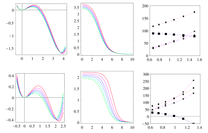
Figure 3: Dependence of effective potential, critical bubble and nucleation rate on the coarse graining scale $k$.

2.3 Two examples

Sample computations are presented in fig. 3. The first row corresponds to a model with an initial potential given by eq. (7) with $m^{2}_{k_{0}}=-0.0433~{}k_{0}^{2}$, $\gamma_{k_{0}}=-0.0634~{}k_{0}^{3/2}$, $\lambda_{k_{0}}=0.1~{}k_{0}$. We first show the evolution of the potential $U_{k}(\phi)$ as the scale $k$ is lowered. The solid line corresponds to $k/k_{0}=0.513$ while the line with longest dashes (that has the smallest barrier height) corresponds to $k_{f}/k_{0}=0.223$. At the scale $k_{f}$ the negative curvature at the top of the barrier is slightly larger than $-k_{f}^{2}$ and we stop the evolution. The potential and the field have been normalized with respect to $k_{f}$. As $k$ is lowered from $k_{0}$ to $k_{f}$, the absolute minimum of the potential settles at a non-zero value of $\phi$, while a significant barrier separates it from the metastable minimum at $\phi=0$. The profile of the critical bubble $\phi_{b}(r)$ is plotted in the second figure in units of $k_{f}$ for the same sequence of scales. For $k\simeq k_{f}$ the characteristic length scale of the bubble profile and $1/k$ are comparable. This is expected, because the form of the profile is determined by the barrier of the potential, whose curvature is $\simeq-k^{2}$ at this point. This is an indication that we should not proceed to coarse-graining scales below $k_{f}$. We observe a significant variation of the value of the field $\phi$ in the interior of the bubble for different $k$.

Our results for the nucleation rate are presented in the third figure. The horizontal axis corresponds to $k/\sqrt{U^{\prime\prime}_{k}(\phi_{t}})$, i.e. the ratio of the scale $k$ to the square root of the positive curvature (equal to the mass of the field) at the absolute minimum of the potential located at $\phi_{t}$. Typically, when $k$ crosses below this mass, the massive fluctuations of the field start decoupling. The evolution of the convex parts of the potential slows down and eventually stops. The dark diamonds give the values of the action $S_{k}$ of the critical bubble. We observe a strong $k$ dependence of this quantity. The stars indicate the values of $\ln(A_{k}/k^{4}_{f})$. Again a substantial decrease with decreasing $k$ is observed. The dark squares give our results for $-\ln(I/k^{4}_{f})=S_{k}-\ln(A_{k}/k^{4}_{f})$. It is remarkable that the $k$ dependence of this quantity almost disappears for $k/\sqrt{U^{\prime\prime}_{k}(\phi_{t}})\mathrel{\vbox{\hbox{$<$}\nointerlineskip\hbox{$\sim$}}}1$. The small residual dependence on $k$ can be used to estimate the contribution of the next order in the expansion around the saddle point. It is reassuring that this contribution is expected to be smaller than $\ln(A_{k}/k^{4}_{f})$.

This behaviour confirms our expectation that the nucleation rate should be independent of the scale $k$ that we introduced as a calculational tool. It also demonstrates that all the configurations plotted in the second figure give equivalent descriptions of the system, at least for the lower values of $k$. This indicates that the critical bubble should not be associated only with the saddle point of the semiclassical approximation, whose action is scale dependent. It is the combination of the saddle point and its possible deformations in the thermal bath that has physical meaning.

For smaller values of $|m^{2}_{k_{0}}|$ the dependence of the nucleation rate on $k$ becomes more pronounced. We demonstrate this in the second row in fig. 3 for which $\lambda_{k_{0}}/(-m^{2}_{k_{0}})^{1/2}$ $=0.88$ (instead of $0.48$ for the first row). The value of $\lambda_{k_{0}}$ is the same as before, whereas $\gamma_{k_{0}}=-1.61\cdot 10^{-3}k_{0}^{3/2}$ and $k_{f}/k_{0}=0.0421$. Higher-loop contributions to $A_{k}$ become important and the expansion around the saddle point does not converge any more. There are two clear indications of the breakdown of the expansion:
a) The values of the leading and subleading contributions to the nucleation rate, $S_{k}$ and $\ln(A_{k}/k^{4}_{f})$ respectively, become comparable.
b) The $k$ dependence of $\ln(I/k^{4}_{f})$ is strong and must be canceled by the higher-order contributions.
The discontinuity in the order parameter at the phase transition is approximately 5 times smaller in the second example than in the first one. As a result, the second phase transition can be characterized as weaker. Typically, the breakdown of the saddle-point approximation is associated with weak first-order phase transitions.

In the last figure of each row we also display the values of $\ln(A_{k}/k^{4}_{f})$ (dark triangles) predicted by the approximate expression

$$\ln\frac{A_{k}}{k^{4}_{f}}\approx\frac{\pi k}{2}\left[-\int_{0}^{\infty}\!\!\!r^{3}\left[U^{\prime\prime}_{k}\left(\phi_{b}(r)\right)-U^{\prime\prime}_{k}\left(0\right)\right]dr\right]^{1/2}.$$ (11)

It gives a good approximation to the exact numerical results, especially near $k_{f}$, and can be used for quick checks of the validity of the expansion around the saddle point.

2.4 Region of validity of homogeneous nucleation theory

It is useful to obtain some intuition on the behaviour of the nucleation rate by using the approximate expression (11). We assume that the potential has a form similar to eq. (7) even near $k_{f}$, i.e.

$$U_{k_{f}}(\phi)\approx\frac{1}{2}m^{2}_{k_{f}}\phi^{2}+\frac{1}{6}\gamma_{k_{f}}\phi^{3}+\frac{1}{8}\lambda_{k_{f}}\phi^{4}.$$ (12)

(Without loss of generality we take $m^{2}_{k_{f}}>0$.) For systems not very close to the endpoint of the first-order critical line, our assumption is supported by the numerical data. The scale $k_{f}$ is determined by the relation

$$k^{2}_{f}\approx\max\left|U^{\prime\prime}_{k_{f}}(\phi)\right|=\frac{\gamma_{k_{f}}^{2}}{6\lambda_{k_{f}}}-m_{k_{f}}^{2}.$$ (13)

Through the rescalings $r=\tilde{r}/m_{k_{f}}$, $\phi=2\tilde{\phi}\,m_{k_{f}}^{2}/\gamma_{k_{f}}$, the potential can be written as $\tilde{U}(\tilde{\phi})=\tilde{\phi}^{2}/2-\tilde{\phi}^{3}/3+h\,\tilde{\phi}^{4}/18$, with $h=9\lambda_{k_{f}}m_{k_{f}}^{2}/\gamma_{k_{f}}^{2}$. For $h\approx 1$ the two minima of the potential have approximately equal depth. The action of the saddle point can be expressed as

$$S_{k_{f}}=\frac{4}{9}\frac{m_{k_{f}}}{\lambda_{k_{f}}}\,h\tilde{S}(h),$$ (14)

where $\tilde{S}(h)$ must be determined numerically through $\tilde{U}(\tilde{\phi})$. Similarly, the pre-exponential factor can be estimated through eq. (11) as

$$\ln\frac{A_{k_{f}}}{k^{4}_{f}} \approx \frac{\pi}{2}\sqrt{\frac{3}{2h}-1}\,\,\tilde{A}(h),$$

$$\tilde{A}^{2}(h) = \int_{0}^{\infty}\left[\tilde{U}^{\prime\prime}\left(\tilde{\phi}_{b}(\tilde{r})\right)-1\right]\,\tilde{r}^{3}\,d\tilde{r},$$ (15)

with $\tilde{A}(h)$ computed numerically. Finally, the relative importance of the fluctuation determinant is given by

$$R=\frac{\ln\left(A_{k_{f}}/k_{f}^{4}\right)}{S_{k_{f}}}\approx\frac{9\pi}{8}\frac{1}{h}\sqrt{\frac{3}{2h}-1}\,\frac{\tilde{A}(h)}{\tilde{S}(h)}\,\frac{\lambda_{k_{f}}}{m_{k_{f}}}=T(h)\,\frac{\lambda_{k_{f}}}{m_{k_{f}}}.$$ (16)

The ratio $R$ can be used as an indicator of the validity of the saddle point expansion. The latter is valid only for $R\mathrel{\vbox{\hbox{$<$}\nointerlineskip\hbox{$\sim$}}}1$.

Numerical evaluation of $T(h)$ shows that it diverges for $h\to 0$, while it becomes small for $h\to 1$. This suggests two cases in which the expansion around the saddle point is expected to break down:
a) For fixed $\lambda_{k_{f}}/m_{k_{f}}$, the ratio $R$ becomes larger than 1 for $h\to 0$. In this limit the barrier becomes negligible and the system is close to the spinodal line.
b) For fixed $h$, $R$ can be large for sufficiently large $\lambda_{k_{f}}/m_{k_{f}}$. This is possible even for $h$ close to 1, so that the system is far from the spinodal line. This case corresponds to weak first-order phase transitions, as can be verified by observing that the saddle-point action  (14), the location of the true vacuum

$$\frac{\phi_{t}}{\sqrt{m_{k_{f}}}}=\frac{2}{3}\sqrt{h}\,\,\tilde{\phi}_{t}(h)\,\sqrt{\frac{m_{k_{f}}}{\lambda_{k_{f}}}},$$ (17)

and the difference in free-energy density between the minima

$$\frac{\Delta U}{m_{k_{f}}^{3}}=\frac{4}{9}\,{h}\,\,\Delta\tilde{U}(h)\,\frac{m_{k_{f}}}{\lambda_{k_{f}}}$$ (18)

go to zero in the limit $m_{k_{f}}/\lambda_{k_{f}}\to 0$ for fixed $h$. This is in agreement with the discussion of fig. 3 in the previous subsection.
The breakdown of homogeneous nucleation theory in both the above cases is confirmed through the numerical computation of the nucleation rates $\!{}^{{\bf?}}$.

2.5 Other results

The approach has been applied to more complicated systems, such as theories of two scalar fields. The most interesting feature of the two-scalar models is the presence of radiatively induced first-order phase transitions. Such transitions usually take place when the expectation value of a certain field generates the mass of another through the Higgs mechanism. The fluctuations of the second field can induce the appearance of new minima in the potential of the first, resulting in first-order phase transitions. We discussed such an example in the first section. The problem of double-counting the effect of fluctuations is particularly acute in such situations. The introduction of a coarse-graining scale $k$ resolves this problem, by separating the high-frequency fluctuations of the system which may be responsible for the presence of the second minimum through the Coleman-Weinberg mechanism $\!{}^{{\bf?}}$, from the low-frequency ones which are relevant for tunnelling.

Unfortunately, the expansion around the saddle point does not converge for radiatively induced first-order phase transitions. The prefactor resulting from the fluctuation determinant of the second field is always comparable to the leading exponential term $\!{}^{{\bf?}}$. As a result, the saddle-point approximation breaks down and the predicted nucleation rate $I/k^{4}_{f}$ is strongly $k$ dependent. The above results are not surprising. The radiative corrections to the potential and the pre-exponential factor have a very similar form of fluctuation determinants. When the radiative corrections are large enough to modify the bare potential and generate a new minimum, the pre-exponential factor should be expected to be important also. These findings have important implications for cosmological phase transitions, such as the electroweak $\!{}^{{\bf?},{\bf?}}$.

Finally, the reliability of our approach has been confirmed through comparisons with results obtained through lattice simulations $\!{}^{{\bf?}}$, or alternative analytical methods in their region of applicability $\!{}^{{\bf?}}$.

References

References

- [1] V.A. Rubakov and M.E. Shaposhnikov, preprint hep-ph/9603208; N. Tetradis, Nucl. Phys. B 488, 92 (1997).
- [2] J. Rudnick, Phys. Rev. B 18, 1406 (1978).
- [3] A. Aharony, in Phase Transitions and Critical Phenomena, vol. 6, eds. C. Domb and M.S. Green (Academic Press, 1976); D.J. Amit, Field Theory, the Renormalization Group and Critical Phenomena (World Scientific, 1984).
- [4] N. Tetradis and C. Wetterich, Nucl. Phys. B 398, 659 (1993); S. Bornholdt, N. Tetradis and C. Wetterich, Phys. Lett. B 348, 89 (1995); Phys. Rev. D 53, 4552 (1996).
- [5] P. Arnold and L.G. Yaffe, Phys. Rev. D 55, 7760 (1997); P. Arnold and Y. Zhang, Phys. Rev. D 55, 7776 (1997).
- [6] P. Arnold and Y. Zhang, Nucl. Phys. B 501, 803 (1997).
- [7] P. Arnold, S.R. Sharpe, L.G. Yaffe and Y. Zhang, Phys. Rev. Lett. 78, 2062 (1997).
- [8] N. Tetradis, Phys. Lett. B 431, 380 (1998).
- [9] C. Wetterich, Nucl. Phys. B 352, 529 (1991); Phys. Lett. B 301, 90 (1993); J. Berges, N. Tetradis and C. Wetterich, preprint hep-ph/0005122.
- [10] N. Tetradis and C. Wetterich, Nucl. Phys. B 422, 541 (1994).
- [11] T. Morris, Nucl. Phys. B 495, 477 (1997).
- [12] J. Berges and C. Wetterich, Nucl. Phys. B 487, 675 (1997); J. Berges, N. Tetradis and C. Wetterich, Phys. Lett. B 393, 387 (1997).
- [13] J. Zinn-Justin, Quantum Field Theory and Critical Phenomena (Oxford Science Publications, 1989).
- [14] J. Langer, Ann. Phys. 41, 108 (1967); Ann. Phys. 54, 258 (1969); Physica 73, 61 (1974).
- [15] S. Coleman, Phys. Rev. D 15, 2929 (1977).
- [16] C.G. Callan and S. Coleman, Phys. Rev. D 16, 1762 (1977).
- [17] I. Affleck, Phys. Rev. Lett. 46, 388 (1981).
- [18] A.D. Linde, Nucl. Phys. B 216, 421 (1983).
- [19] S. Coleman and E. Weinberg, Phys. Rev. D 7, 1888 (1973).
- [20] A. Strumia and N. Tetradis, Nucl. Phys. B 542, 719 (1999).
- [21] A. Strumia, N. Tetradis and C. Wetterich, Phys. Lett. B 467, 279 (1999).
- [22] A. Strumia and N. Tetradis, Nucl. Phys. B 554, 697 (1999).
- [23] A. Strumia and N. Tetradis, Nucl. Phys. B 560, 482 (1999).
- [24] A. Strumia and N. Tetradis, JHEP 9911, 023 (1999).
- [25] G. Münster, A. Strumia and N. Tetradis, Phys. Lett. A 271, 80 (2000).