Absence of higher order corrections to the non-Abelian topological mass term

Abstract

We study the Yang-Mills-Chern-Simons theory systematically in an effort to generalize the Coleman-Hill result to the non-Abelian case. We show that, while the Chern-Simons coefficient is in general gauge dependent in a non-Abelian theory, it takes on a physical meaning in the axial gauge. Using the non-Abelian Ward identities as well as the analyticity of the amplitudes in the momentum variables, we show that, in the axial gauge, the Chern-Simons coefficient does not receive any quantum correction beyond one loop. This allows us to deduce that the ratio ${4\pi m\over g^{2}}$ is unrenormalized, in a non-Abelian theory, beyond one loop in any infrared safe gauge. This is the appropriate generalization of the Coleman-Hill result to non-Abelian theories. Various other interesting properties of the theory are also discussed.

1 Introduction:

It is well known by now that in odd space-time dimensions, one can add a topological term to the Lagrangian density of a gauge field, in addition to the usual Yang-Mills (Maxwell) term. Such a term is known as the Chern-Simons term and a theory with a Chern-Simons term is conventionally called a Chern-Simons theory [1, 2]. In $2+1$ dimensions, for example, the Chern-Simons term, in a $SU(N)$ gauge theory, has the form

$${\cal L}_{CS}={m\over 2}\,\epsilon^{\mu\nu\lambda}\,A_{\mu}^{a}(\partial_{\nu}A_{\lambda}^{a}+{g\over 3}f^{abc}A_{\nu}^{b}A_{\lambda}^{c})$$

where $g$ represents the gauge coupling and $f^{abc}$ stand for the structure constants of the group. The parameter $m$ is known as the Chern-Simons coefficient (at the tree level) and has the dimensions of mass. In a theory, with a Yang-Mills term for the gauge fields, it can be shown that the Chern-Simons term provides a gauge invariant mass for the gauge fields. Such a mass term is absolutely crucial in the perturbative study of a pure Yang-Mills-Chern-Simons gauge theory, since without this term, the infrared divergences in $2+1$ dimensions are so severe that a perturbative expansion cannot be defined [2, 3].

The Chern-Simons term violates discrete symmetries like $P$ and $T$ (although it respects $CPT$). In a gauge theory with (matter) interactions which violate these symmetries, it is expected that a Chern-Simons term will be generated at the quantum level, even if one is not present at the tree level. Thus, for example, the mass term for a fermion, in $2+1$ dimensions, is known to violate these symmetries and, correspondingly, it is known that a massive fermion interacting with gauge fields generates a Chern-Simons term at the one loop level [2]. Surprisingly, however, it was noted, through explicit calculations, that even though a Chern-Simons term is generated at one loop, there is no radiative correction to the Chern-Simons coefficient at the two loop level, either in the Abelian or in the non-Abelian theory [4, 5]. This peculiarity was explained, for the Abelian theory, by Coleman and Hill, who showed that, in $2+1$ dimensional QED with or without a tree level Chern-Simons term, the Chern-Simons coefficient does not receive any contribution beyond one loop at zero temperature [6]. The proof of this result is quite elegant and essentially uses two key assumptions, namely, i) the Abelian Ward identity and, ii) the analyticity of the amplitudes in the momentum (energy-momentum) variables. This result holds, in an Abelian theory, whenever these assumptions are valid, but not otherwise.

While the Coleman-Hill result explains the peculiarity of the explicit two loop calculation in the Abelian theory, it says nothing about the outcome of the calculation in the non-Abelian theory. There are, in fact, several difficulties one faces in trying to extend the Coleman-Hill result to non-Abelian theories. First, unlike in an Abelian theory at zero temperature, without a tree level Chern-Simons term, infrared divergences may be too severe (as we have already mentioned). Second, even with a tree level Chern-Simons term in the non-Abelian theory, an arbitrary gauge choice may introduce spurious infrared divergences and, therefore, one must carefully choose an infrared safe gauge [2, 7] (again, this is not a problem in the Abelian theory). Finally, in the non-Abelian theory, the Chern-Simons coefficient is, in general, gauge dependent (in an Abelian theory, this coefficient is gauge independent). Therefore, an attempt to naively generalize the Coleman-Hill result is meaningless. On the other hand, it is known that, in a non-Abelian theory, the ratio ${4\pi m\over g^{2}}$ is gauge independent and has a physical significance. Consequently, it makes sense to try and show that it is this ratio which gets no contribution beyond one loop in a non-Abelian theory.

In this paper, we show that this expectation, indeed, holds. In particular, we show, much like the Coleman-Hill result in the Abelian theory, that if, i) the Ward identities of the non-Abelian theory hold and, ii) the amplitudes are analytic in the momentum (energy-momentum) variables, then the ratio ${4\pi m\over g^{2}}$ does not receive any quantum correction beyond one loop. The non-Abelian theory is clearly much more complicated than the Abelian counterpart and we prove our result by working in the axial gauge, which is an infrared safe gauge. It is, of course, known that the Ward identities in the axial gauge are much simpler, but we show that, in this gauge, the Chern-Simons coefficient takes on a physical significance, although it is gauge dependent in general. In fact, we show that the Chern-Simons coefficient, in the axial gauge, receives no quantum correction beyond one loop and this allows us to deduce that the ratio ${4\pi m\over g^{2}}$ is unaffected beyond one loop. A brief account of our main result has already been published [8] and here we describe the details of our work along with many other interesting features of the analysis.

The organization of our paper is as follows. In section 2, we analyze the Yang-Mills-Chern-Simons theory in a covariant gauge and show, using a Nielsen-like identity [9, 10], that the Chern-Simons coefficient is, in general, gauge dependent. In section 3, we define the theory in the axial gauge and discuss some of the special features of this gauge choice. From the Ward identities, in this gauge, we obtain a diagrammatic representation for the Chern-Simons coefficient, which is quite useful in an all order proof. We also show that, in this gauge, the Chern-Simons coefficient takes on a physical meaning and derive a Nielsen-like identity to show that it is independent of $n^{\mu}$, the choice of direction in the axial gauge. In section 4, we explicitly evaluate the Chern-Simons coefficient at one loop and show that it is independent of $n^{\mu}$ as is required from the Nielsen-like identity described in section 3. We compare our calculation with that in the Landau gauge [7] to bring out the gauge independent nature of the ratio ${4\pi m\over g^{2}}$. We also present an interpolating gauge that interpolates between the infrared safe Landau and axial gauges. In section 5 we prove the main result of our paper, namely that, with the assumptions of BRST invariance and analyticity of the amplitudes, the Chern-Simons coefficient has no quantum correction beyond one loop in the axial gauge. We deduce from this that, in any infrared safe gauge, the ratio ${4\pi m\over g^{2}}$ receives no radiative correction beyond one loop. In section 6, we study the pure Chern-Simons theory (without a Yang-Mills term) and show that it has an additional vector supersymmetry in the axial gauge (much like the one in the Landau gauge). The Ward identities following from this, together with the usual Ward identities show that this is a free theory. We present a brief conclusion in section 7.

2 Gauge Dependence:

Let us consider the Yang-Mills-Chern-Simons theory in $2+1$ dimensions described by the Lagrangian density [2, 7, 11, 12, 13]

$${\cal L}_{inv}={1\over 2}{\rm tr}\,F_{\mu\nu}F^{\mu\nu}-m\,{\rm tr}\,\epsilon^{\mu\nu\lambda}A_{\mu}(\partial_{\nu}A_{\lambda}+{2\,g\over 3}A_{\nu}A_{\lambda})$$ (1)

where we have chosen, for simplicity, the Chern-Simons mass $m$ to be positive. The gauge field belongs to a matrix representation of $SU(N)$,

$$A_{\mu}=A_{\mu}^{a}T^{a}$$

with the generators of the group assumed to have the normalization

$${\rm tr}\,T^{a}T^{b}=-{1\over 2}\delta^{ab}$$

and

$$F_{\mu\nu}=\partial_{\mu}A_{\nu}-\partial_{\nu}A_{\mu}+g[A_{\mu},A_{\nu}].$$

This is a self-interacting theory and one can, of course, add to it interacting matter fields. However, we would restrict ourselves, for simplicity, to the theory described by Eq. (1), which can be written with explicit internal symmetry indices as

$${\cal L}_{inv}=-{1\over 4}F^{\mu\nu,a}F_{\mu\nu}^{a}+{m\over 2}\epsilon^{\mu\nu\lambda}A_{\mu}^{a}(\partial_{\nu}A_{\lambda}^{a}+{g\over 3}f^{abc}A_{\nu}^{b}A_{\lambda}^{c})$$ (2)

The Lagrangian density, in Eq. (1), is invariant under the infinitesimal $SU(N)$ gauge transformations of the form

$$\delta A_{\mu}(x)=D_{\mu}\epsilon(x)=\partial_{\mu}\epsilon(x)+g[A_{\mu},\epsilon]$$

where $\epsilon(x)$ is an infinitesimal matrix valued transformation parameter. On the other hand, under a finite gauge transformation

$$A_{\mu}\rightarrow U^{-1}A_{\mu}U-{i\over g}U^{-1}\partial_{\mu}U$$

the Lagrangian density changes by a total divergence (it is the Chern-Simons term that is not invariant), so that the action changes by a constant

$$S_{inv}=\int d^{3}x\,{\cal L}_{inv}\rightarrow S_{inv}+{4\pi m\over g^{2}}\,2\pi W$$ (3)

where

$$W={1\over 24\pi^{2}}\int d^{3}x\,\epsilon^{\mu\nu\lambda}\,{\rm tr}U^{-1}\partial_{\mu}UU^{-1}\partial_{\nu}UU^{-1}\partial_{\lambda}U$$ (4)

is an integer, known as the winding number of the gauge transformation, and classifies the gauge transformations into topologically distinct classes. When the winding number vanishes, the gauge transformations are conventionally known as small gauge transformations, while non zero winding numbers lead to large gauge transformations. It is clear from Eq. (3) that under a small gauge transformation, the action is invariant, while, under a large gauge transformation, the action changes by a constant. In the path integral approach, it is quite clear that even though there is a shift in the action under a large gauge transformation, the generating functional is invariant provided

$${4\pi m\over g^{2}}=n$$ (5)

where $n$ is a positive integer (because of our choice $m>0$).

It is well known that the coefficient of the Chern-Simons term (which is $m$ in the tree level), in an Abelian theory, is a gauge independent quantity. It is related to the physically meaningful statistics parameter and, in fact, it is this coefficient which does not receive quantum corrections beyond one-loop (provided certain assumptions are valid) according to the Coleman-Hill result. In trying to extend this result to non-Abelian theories, one of the challenges we face, as mentioned in the introduction, is that the Chern-Simons coefficient is, in general, a gauge dependent quantity in a non-Abelian theory. This is best seen from the following analysis involving a Nielsen-like identity [9, 10].

Let us analyze the Chern-Simons theory in a general covariant gauge. Thus, adding a gauge fixing and ghost Lagrangian density of the form

$${\cal L}_{gf}+{\cal L}_{ghost} = -{1\over 2\xi}(\partial_{\mu}A^{\mu,a})^{2}+\partial^{\mu}\overline{c}^{a}D_{\mu}c^{a}$$ (6)

$$= {\xi\over 2}F^{a}F^{a}-F^{a}(\partial_{\mu}A^{\mu,a})+\partial^{\mu}\overline{c}^{a}D_{\mu}c^{a}$$

we can write the total Lagrangian density, in this gauge, to be

$${\cal L}={\cal L}_{inv}+{\cal L}_{gf}+{\cal L}_{ghost}$$ (7)

We note that we have introduced an auxiliary field, $F^{a}$, to write the gauge fixing term, which helps close the algebra of the BRST charges off-shell. From the BRST identities for the theory, in this gauge, one knows that the gauge fixing parameter, $\xi$, is not renormalized so that we can parameterize the two point function of the full theory as

$$\begin{array}[]{ll}\Pi^{\mu\nu,ab}(p)=\delta^{ab}&\left[\right.(p^{\mu}p^{\nu}-\eta^{\mu\nu}p^{2})(1+\Pi_{1}(p))\\ &\\ &+i\,m\epsilon^{\mu\nu\lambda}p_{\lambda}(1+\Pi_{2}(p))-\displaystyle{1\over\xi}p^{\mu}p^{\nu}\left.\right]\end{array}$$ (8)

Here, $\Pi_{1}(p)$ and $\Pi_{2}(p)$ represent, respectively, the radiative corrections to the parity conserving transverse part and the parity violating part of the two point function. It is worth noting from this that the Chern-Simons coefficient, at any order, can be obtained from the two point function as

$$\delta^{ab}\overline{\Pi}_{2}(0)=\delta^{ab}(1+\Pi_{2}(0))={1\over 6im}\,\epsilon_{\mu\nu\lambda}\,\left.{\partial\over\partial p_{\lambda}}\Pi^{\mu\nu,ab}(p)\right|_{p=0}$$ (9)

We note that it is $m\overline{\Pi}_{2}(0)$ which represents the complete Chern-Simons coefficient, with $m\Pi_{2}(0)$ representing the part coming from quantum corrections. Let us also note here that, in this gauge, the tree level propagator for the gauge field has the form

$$D_{\mu\nu}^{(0)ab}(p)=\delta^{ab}\left[{1\over p^{2}-m^{2}}\left\{\left(\eta_{\mu\nu}-{p_{\mu}p_{\nu}\over p^{2}}\right)+im\,\epsilon_{\mu\nu\lambda}\,{p^{\lambda}\over p^{2}}\right\}+{\xi p_{\mu}p_{\nu}\over(p^{2})^{2}}\right]$$ (10)

To study the gauge dependence of the Chern-Simons coefficient, let us add to the Lagrangian the following source terms

$${\cal L}_{total}={\cal L}+{\cal L}_{source}$$ (11)

where

$${\cal L}_{source} = J^{\mu,a}A_{\mu}^{a}+J^{a}F^{a}+i(\overline{\eta}^{a}c^{a}-\overline{c}^{a}\eta^{a})+K^{\mu,a}D_{\mu}c^{a}$$ (12)

$$\quad+L^{a}(-{1\over 2}f^{abc}c^{b}c^{c})+{1\over 2}HF^{a}\overline{c}^{a}$$

Here, all the sources are the standard ones, introduced to derive and study BRST identities, except for the last term whose role would become clear shortly.

We note that, under a BRST transformation ($\omega$ is a space-time independent anti-commuting parameter),

$$\delta A_{\mu}^{a} = \omega D_{\mu}c^{a}$$

$$\delta c^{a} = -{\omega\over 2}\,f^{abc}c^{b}c^{c}$$

$$\delta\overline{c}^{a} = -\omega F^{a}$$

$$\delta F^{a} = 0$$ (13)

the source terms are not invariant although ${\cal L}$ is. In fact, we obtain

$$\delta{\cal L}_{source}=\omega\left[J^{\mu,a}(D_{\mu}c^{a})-i\overline{\eta}^{a}(-{1\over 2}f^{abc}c^{b}c^{c})+iF^{a}\eta^{a}+{1\over 2}HF^{a}F^{a}\right]$$ (14)

Making a field redefinition inside the path integral which coincides with a BRST transformation, then, we obtain from the invariance of the generating functional

$$Z=e^{iW}=\int{\cal D}A_{\mu}^{a}{\cal D}F^{a}{\cal D}\overline{c}^{a}{\cal D}c^{a}\,e^{i\int d^{3}x\,{\cal L}_{total}}$$

the master identity

$${\partial W\over\partial\xi} = \int d^{3}x\,d^{3}y\left(J^{\mu,a}(x){\delta^{2}W\over\delta K^{\mu,a}(x)\delta H(y)}-i\overline{\eta}^{a}(x){\delta^{2}W\over\delta L^{a}(x)\delta H(y)}\right.$$ (15)

$$\qquad\qquad\qquad\left.-i{\delta^{2}W\over\delta J^{a}(x)\delta H(y)}\eta^{a}(x)\right)$$

In other words, this identity allows us to study the gauge dependence of the effective action.

We can now make a Legendre transformation (with respect to the usual sources $J^{\mu,a},J^{a},\eta^{a},\overline{\eta}^{a}$) and go to the effective action and the identity above takes the form

$${\partial\Gamma\over\partial\xi} = -\int d^{3}x\,d^{3}y\left({\delta\Gamma\over\delta A_{\mu}^{a}(x)}{\delta^{2}\Gamma\over\delta K^{\mu,a}(x)\delta H(y)}+{\delta\Gamma\over\delta c^{a}(x)}{\delta^{2}\Gamma\over\delta L^{a}(x)\delta H(y)}\right.$$ (16)

$$\qquad\qquad\qquad\left.-{\delta F^{a}(x)\over\delta H(y)}{\delta\Gamma\over\delta\overline{c}^{a}(x)}\right)$$

This identity describes the gauge dependence of the effective action and we can derive the gauge dependence of any 1PI amplitude from this. In particular, we note that (see Eq. (9))

$${\partial\overline{\Pi}_{2}(0)\over\partial\xi}=\left.{1\over 6\,im\,(N^{2}-1)}\,\epsilon_{\mu\nu\rho}{\partial\over\partial\xi}{\partial\over\partial p_{\rho}}{\delta^{2}\Gamma\over\delta A_{\mu}^{a}(p)\delta A_{\nu}^{a}(-p)}\right|_{p=0}$$

$$=-{1\over 6\,im\,(N^{2}-1)}\,\epsilon_{\mu\nu\rho}{\partial\over\partial p_{\rho}}\left[{\delta^{3}\Gamma\over\delta A_{\mu}^{a}(p)\delta A_{\nu}^{a}(-p)\delta A_{\lambda}^{b}(0)}{\delta^{2}\Gamma\over\delta K^{\lambda,b}(0)\delta H(0)}\right.$$

$$\qquad+{\delta^{2}\Gamma\over\delta A_{\mu}^{a}(p)\delta A_{\lambda}^{b}(-p)}{\delta^{3}\Gamma\over\delta A_{\nu}^{a}(-p)\delta K^{\lambda,b}(p)\delta H(0)}$$

$$\qquad\left.\left.+{\delta^{2}\Gamma\over\delta A_{\nu}^{a}(-p)\delta A_{\lambda}^{b}(p)}{\delta^{3}\Gamma\over\delta A_{\mu}^{a}(p)\delta K^{\lambda,b}(-p)\delta H(0)}\right]\right|_{p=0}$$ (17)

Here, we are supposed to also understand that all fields are set to zero after evaluating the functional derivatives.

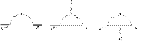
Figure 1: One loop diagrams that can lead to a mixing of the sources. The wavy lines represent gauge fields, the solid line, the auxiliary field $F^{a}$, and the dashed lines stand for ghosts.

There are several things to note from this. First, there are no tree level mixing terms of the forms $K^{\mu,a}H,K^{\mu,a}A_{\nu}^{b}H$ so that the gauge dependence of the Chern-Simons coefficient can only arise from radiative corrections. One can explicitly check at one loop level and argue from symmetry arguments that radiative corrections cannot generate a vertex of the form $K^{\mu,a}H$ (for such a vertex, the colour index cannot be saturated). Consequently, the first term on the right hand side of Eq. (17) does not contribute. At one loop, a vertex of the form $K^{\mu,a}(p)A_{\nu}^{b}(-p)H(0)$ is already generated (see Fig. 1). Therefore, let us parameterize such a vertex as,

$$\left.{\delta^{3}\Gamma\over\delta K^{\mu,a}(p)\delta A_{\nu}^{b}(-p)\delta H(0)}\right|=\delta^{ab}\left[\delta_{\mu}^{\nu}A(p)+p_{\mu}p^{\nu}B(p)+i\epsilon_{\mu}^{\;\nu\lambda}p_{\lambda}C(p)\right]$$ (18)

Substituting this into the identity (17), we obtain,

$${\partial\overline{\Pi}_{2}(0)\over\partial\xi}=2(1+\Pi_{2}(0))A(0)$$ (19)

The right hand side can be evaluated order by order and, in general, is not zero showing that the Chern-Simons coefficient, in a non-Abelian theory is, in general, gauge dependent. We also note that $A(0)$ is obtained from the vertex $K^{\mu,a}A_{\nu}^{b}H$ with all external momenta equal to zero. Consequently, this has severe infrared divergences and unless an infrared safe gauge, like the Landau gauge, is chosen, the identities cannot even be satisfied.

3 Axial gauge:

In the previous section, we saw that the Chern-Simons coefficient is, in general, gauge dependent. Therefore, this naturally raises the question as to whether the Coleman-Hill result can even be meaningfully generalized to non-Abelian theories and if so, in what manner. In this section, we will show that, in the axial gauge, the Chern-Simons coefficient has a physical significance and, therefore, this is possibly the appropriate gauge in which to consider a generalization of the Coleman-Hill analysis.

Let us consider a general axial gauge [14] described by a gauge fixing and ghost Lagrangian density of the form

$${\cal L}_{gf}+{\cal L}_{ghost} = -{1\over 2\xi}(n^{\mu}A_{\mu}^{a})^{2}-\overline{c}^{a}n^{\mu}(D_{\mu}c^{a})$$ (20)

$$= {\xi\over 2}F^{a}F^{a}-F^{a}(n^{\mu}A_{\mu}^{a})-\overline{c}^{a}n^{\mu}(D_{\mu}c^{a})$$

Here, $n^{\mu}$ represents an arbitrary direction. The theory described by

$${\cal L}={\cal L}_{inv}+{\cal L}_{gf}+{\cal L}_{ghost}$$ (21)

is infrared divergent in $2+1$ dimensions, unless $\xi=0$ and we will study the theory in such a limiting gauge. For $\xi=0$, $n^{2}=n^{\mu}n_{\mu}=0$ defines the light-cone gauge, while $n^{2}\geq 0$ leads to the time-like axial gauge and so on.

The tree level propagator of the gauge field for an arbitrary gauge fixing parameter $\xi$ is given by

$$D^{(0)ab}_{\mu\nu}(p) = {\delta^{ab}\over p^{2}-m^{2}}\left[\eta_{\mu\nu}-{n_{\mu}p_{\nu}+n_{\nu}p_{\mu}\over(n\cdot p)}+{n^{2}p_{\mu}p_{\nu}\over(n\cdot p)^{2}}+im\epsilon_{\mu\nu\lambda}{n^{\lambda}\over(n\cdot p)}\right]$$ (22)

$$\qquad\qquad\qquad+{\delta^{ab}\xi p_{\mu}p_{\nu}\over(n\cdot p)^{2}}$$

From this, we obtain the tree level propagator, in the axial gauge ($\xi=0$), to be

$$D^{(0)ab}_{\mu\nu}(p)={\delta^{ab}\over p^{2}-m^{2}}\left[\eta_{\mu\nu}-{n_{\mu}p_{\nu}+n_{\nu}p_{\mu}\over(n\cdot p)}+{n^{2}p_{\mu}p_{\nu}\over(n\cdot p)^{2}}+im\epsilon_{\mu\nu\lambda}{n^{\lambda}\over(n\cdot p)}\right]$$ (23)

which can be trivially checked to be transverse to $n^{\mu}$, namely,

$$n^{\mu}D^{(0)ab}_{\mu\nu}(p)=0=D^{(0)ab}_{\mu\nu}(p)n^{\nu}$$ (24)

This observation is quite significant as we will see shortly.

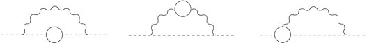
Figure 2: Diagrams, which can contribute to the ghost self-energy, vanish because of Eq. (24).

Let us note that the theory described by Eq. (21) is also invariant under the BRST transformations of Eq. (13). Thus, one can derive, as usual (by adding sources as in Eq. (12) except for the last source), the BRST identities for the theory, which are derived from the master identity

$$\int d^{3}x\,\left({\delta\Gamma\over\delta A_{\mu}^{a}(x)}{\delta\Gamma\over\delta K^{\mu,a}(x)}-{\delta\Gamma\over\delta c^{a}(x)}{\delta\Gamma\over\delta L^{a}(x)}+F^{a}(x){\delta\Gamma\over\delta\overline{c}^{a}(x)}\right)=0$$ (25)

The master identity is the same as in any other gauge. However, the constraints following from them, in the axial gauge, are much simpler than, say in a covariant gauge. For example, looking at the structure of the ghost Lagrangian in Eq. (20), we note that, in the axial gauge, the vertex describing the coupling of the ghosts to the gluons is proportional to $n^{\mu}$. Combined with Eq. (24), this, then, implies that, in the axial gauge, the ghost two point function does not receive any quantum correction. As a result, in this gauge, the ghost wave function renormalization is trivial,

$$\widetilde{Z}_{3}=1$$ (26)

Similarly, it also follows that, in this gauge, the ghost-gluon interaction vertex is not renormalized, leading to

$$\widetilde{Z}_{1}=1$$ (27)

As a result, the standard relation following from the master identity in Eq. (25), in a non-Abelian gauge theory, takes the simple form

$${Z_{1}\over Z_{3}} = {\widetilde{Z}_{1}\over\widetilde{Z}_{3}}$$

$${\rm or,}\quad Z_{1} = Z_{3}$$ (28)

Here, we have denoted the wave function and the vertex renormalizations for the gauge field by $Z_{3}$ and $Z_{1}$ respectively. This relation is reminiscent of the Ward identity in an Abelian theory. Thus, in the axial gauge, the Ward identities are simpler, much like in the Abelian theory. However, the non-Abelian interactions still make the structure of any amplitude much more complex and rich.

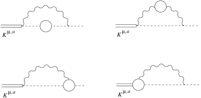
Figure 3: Diagrams, which can lead to the renormalization of the $K^{\mu,\,a}\,c^{a}$ vertex, vanish because of Eq. (24).

Just as we see that the ghost wave function as well as the ghost vertex renormalizations are trivial in the axial gauge, it is equally straightforward to show that the source terms with composite variations are not renormalized in the axial gauge either (namely, vertices involving the sources $K^{\mu,a}$ and $L^{a}$ receive no quantum correction). As a result, the Ward identities following from the master identity in Eq. (25) take a much simpler form in the axial gauge. For example, it follows from Eq. (25) that, for $n\geq 2$,

$${\delta^{n}\Gamma\over\delta A_{\mu_{1}}^{a_{1}}(p_{1})\cdots\delta A_{\mu_{n-1}}^{a_{n-1}}(p_{n-1})\delta A_{\mu_{n}}^{a}(p_{n})}{\delta^{2}\Gamma\over\delta K^{\mu_{n},a}(-p_{n})\delta c^{a_{n}}(p_{n})}$$

$$= -\sum_{i=1}^{n-1}\int d^{3}p{\delta^{n-1}\Gamma\over\delta A_{\mu_{1}}^{a_{1}}(p_{1})\cdots\delta A_{\mu_{i-1}}^{a_{i-1}}(p_{i-1})\delta A_{\mu_{i+1}}^{a_{i+1}}(p_{i+1})\cdots\delta A_{\mu_{n}}^{a}(p)}$$

$$\qquad\qquad\quad\times{\delta^{3}\Gamma\over\delta K^{\mu_{n},a}(-p)\delta A_{\mu_{i}}^{a_{i}}(p_{i})\delta c^{a_{n}}(p_{n})}$$

Recalling that the vertices with the sources $K^{\mu,a}$ do not get any quantum correction, this identity can also be rewritten in the simple form

$$p_{n,\mu_{n}}\Gamma_{a_{1}\cdots a_{n}}^{\mu_{1}\cdots\mu_{n}}(p_{1},\cdots,p_{n})=$$

$$\!\!ig\!\sum_{i=1}^{n-1}f^{aa_{i}a_{n}}\Gamma^{\mu_{1}\cdots\mu_{n-1}}_{a_{1}\cdots a_{i-1}aa_{i+1}\cdots a_{n-1}}(p_{1},\cdots,p_{i-1},p_{i}+p_{n},p_{i+1},\cdots,p_{n-1})$$ (29)

This is clearly a much simpler identity, relating successive vertex functions, than the identities one obtains, for example, in a covariant gauge. Furthermore, let us note that taking the derivative with respect to $p_{n}$ and setting $p_{n}=0$ in Eq. (29), we obtain

$$\Gamma^{\mu_{1}\cdots\mu_{n}}_{a_{1}\cdots a_{n}}(p_{1},\cdots,p_{n-1},0)=$$ (30)

$$ig\sum_{i=1}^{n-1}f^{aa_{i}a_{n}}{\partial\over\partial p_{i,\mu_{n}}}\Gamma^{\mu_{1}\cdots\mu_{n-1}}_{a_{1}\cdots a_{i-1}aa_{i+1}\cdots a_{n-1}}(p_{1},\cdots,p_{n-1})$$

The two point function in the full theory, in a generalized axial gauge ($\xi\neq 0$), can be parameterized, consistent with the BRST identities, as

$$\Pi^{\mu\nu,ab}(p) = \delta^{ab}\left[-\left(\eta^{\mu\nu}-p^{\mu}p^{\nu}\right)(1+\Pi_{1}(p))+im\epsilon^{\mu\nu\lambda}p_{\lambda}(1+\Pi_{2}(p))\right.$$ (31)

$$\qquad\left.+(p^{\mu}-{p^{2}n^{\mu}\over(n\cdot p)})(p^{\nu}-{p^{2}n^{\nu}\over(n\cdot p)})\Pi_{3}(p)-{1\over\xi}n^{\mu}n^{\nu}\right]$$

The self-energy (which, by definition, is the two point function without the tree level terms) is clearly transverse with respect to momentum. Let us note that relation (3) must hold for both parity conserving as well as parity violating parts of the amplitudes separately. Thus, looking at the parity violating part of the three point amplitude, we obtain, (Note that we have identified $\Gamma^{\mu\nu,ab}=\Pi^{\mu\nu,ab}$.)

$$\epsilon_{\mu\nu\lambda}\Gamma^{\mu\nu\lambda}_{abc} = igf^{dbc}\epsilon_{\mu\nu\lambda}\left.{\partial\over\partial p_{\lambda}}\Pi^{\mu\nu,ad}(p)\right|_{p=0}$$

$${\rm or,}\quad f^{abc}(1+\Pi_{2}(0)) = {1\over 6im}f^{dbc}\epsilon_{\mu\nu\lambda}\left.{\partial\over\partial p_{\lambda}}\Pi^{\mu\nu,da}(p)\right|_{p=0}$$ (32)

$$= {1\over 6mg}\epsilon_{\mu\nu\lambda}\Gamma^{\mu\nu\lambda}_{abc}(0,0,0)$$

This relation is quite crucial in that it relates the Chern-Simons coefficient in the axial gauge, at any order, to the parity violating part of the three gluon vertex (with vanishing momenta) at the same order. Thus, one can give a diagrammatic representation for the Chern-Simons coefficient in the axial gauge, which is very convenient for studying an all order proof of the generalization of the Coleman-Hill result to non-Abelian theories. It is also clear from this identification that the choice of an infrared safe gauge is crucial because the Chern-Simons coefficient is related to the three gluon amplitude with all external momenta vanishing.

In a non-Abelian Chern-Simons theory, as we have argued earlier, the ratio ${4\pi m\over g^{2}}$ represents a physical quantity. This is known to be true from the following facts, namely, in the leading order in ${1\over m}$ expansion, i) it is this ratio which determines the dimensionality of the Chern-Simons Hilbert space [15] and ii) this ratio is related to the coefficient of the WZWN action which represents the central charge of the corresponding current algebra [16]. It is also this ratio (see Eq. (5)) which needs to be quantized for large gauge invariance of the theory. In the full quantum theory, however, this ratio changes as

$${4\pi m\over g^{2}}\rightarrow\left({4\pi m\over g^{2}}\right)_{\rm ren}=Z_{m}\left({Z_{3}\over Z_{1}}\right)^{2}\left({4\pi m\over g^{2}}\right)$$ (33)

where $Z_{3}$ and $Z_{1}$ are the wave function and the vertex renormalization constants for the gauge field (as we have defined earlier), while $Z_{m}$ represents the renormalization of the Chern-Simons coefficient. By definition, of course, $Z_{m}=(1+\Pi_{2}(0))$ and since in the axial gauge we have $Z_{1}=Z_{3}$ (see Eq. (28)), it follows that

$$\left({4\pi m\over g^{2}}\right)_{\rm ren}=Z_{m}\left({4\pi m\over g^{2}}\right)=(1+\Pi_{2}(0))\left({4\pi m\over g^{2}}\right)$$ (34)

Since this is a physical quantity, it follows that, in the axial gauge, the induced Chern-Simons coefficient takes on a physical meaning.

In fact, let us next show that this expectation is indeed true and that the Chern-Simons coefficient is independent of $n^{\mu}$ in the axial gauge. To prove this, let us add to our Lagrangian density the following source terms.

$${\cal L}_{source} = J^{\mu,a}A_{\mu}^{a}+J^{a}F^{a}+i(\overline{\eta}^{a}c^{a}-\overline{c}^{a}\eta^{a})+K^{\mu,a}D_{\mu}c^{a}$$ (35)

$$\qquad+L^{a}(-{1\over 2}f^{abc}c^{b}c^{c})+H^{\mu}\overline{c}^{a}A_{\mu}^{a}$$

Thus, defining

$${\cal L}_{total}={\cal L}+{\cal L}_{source}$$

we note that, under a BRST transformation (see Eq. (13)),

$$\delta{\cal L}_{total}=\omega\left[J^{\mu,a}(D_{\mu}c^{a})-i\overline{\eta}^{a}(-{1\over 2}f^{abc}c^{b}c^{c})+iF^{a}\eta^{a}+H^{\mu}{\partial{\cal L}_{total}\over\partial n^{\mu}}\right]$$ (36)

Thus, as before, making a field redefinition inside the path integral, which coincides with a BRST transformation, we can derive the equation which describes how the effective action changes with $n^{\mu}$. Let us simply note the result here,

$${\partial\Gamma\over\partial n^{\mu}} = -\int d^{3}p\left[{\delta\Gamma\over\delta A_{\nu}^{a}(-p)}{\delta^{2}\Gamma\over\delta K^{\nu,a}(p)\delta H^{\mu}(-p)}+{\delta F^{a}(p)\over\delta H^{\mu}(p)}{\delta\Gamma\over\delta\overline{c}^{a}(-p)}\right.$$ (37)

$$\qquad\qquad\left.-{\delta\Gamma\over\delta c^{a}(-p)}{\delta^{2}\Gamma\over\delta L^{a}(p)\delta H^{\mu}(-p)}\right]$$

This is the master identity from which we obtain,

$${\partial\over\partial n^{\rho}}\left(\epsilon_{\mu\nu\lambda}{\delta^{3}\Gamma\over\delta A_{\mu}^{a}\delta A_{\nu}^{b}\delta A_{\lambda}^{c}}\right)_{p_{1},p_{2},p_{3}=0}=-\epsilon_{\mu\nu\lambda}\left[{\delta^{4}\Gamma\over\delta A_{\mu}^{a}\delta A_{\nu}^{b}\delta A_{\lambda}^{c}\delta A_{\sigma}^{d}}{\delta^{2}\Gamma\over\delta K^{\sigma,d}\delta H^{\rho}}\right.$$

$$+\left.{\delta^{3}\Gamma\over\delta A_{\mu}^{a}\delta A_{\nu}^{b}\delta A_{\sigma}^{d}}{\delta^{3}\Gamma\over\delta K^{\sigma,d}\delta H^{\rho}\delta A_{\lambda}^{c}}\right]_{p_{1},p_{2},p_{3}=0}+{\rm permutations}$$ (38)

where the restriction on the right hand side stands for setting all the field variables as well as momenta equal to zero.

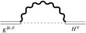
Figure 4: Diagram representing the possible mixing of the sources $K^{\mu,\,a}$ and $H^{\nu}$. The bold wavy line represents the complete gauge field propagator. The diagram vanishes because of color identities.

It is easy to see that, to all orders in the quantum theory, we cannot have a vertex of the form $K^{\mu,a}H^{\nu}$. In fact, let us recall that in the axial gauge the ghost propagator as well as the ghost vertex do not renormalize. Similarly, just as we noted that the vertices involving the source $K^{\mu,a}$ do not renormalize, we can also show that the vertex involving $H^{\mu}$ does not renormalize in the quantum theory either. It follows from this that the only diagram that can give rise to a mixing of the sources $K^{\mu,a}$ and $H^{\nu}$ is as shown in Fig. 4. From the fact that the vertex $K^{\mu,a}A_{\nu}^{b}c^{c}$ is anti-symmetric in the internal indices while the vertex $H^{\mu}A_{\nu}^{a}c^{b}$ and the gauge propagator are symmetric in the internal symmetry indices, it follows that this diagram vanishes. (Alternately, such a vertex, if it existed, would involve a single internal index, which is impossible to construct from the structures present in the theory.)

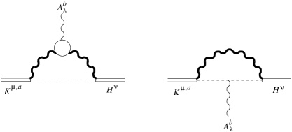
Figure 5: Diagrams contributing to a vertex of the type $K_{\mu}^{a}\,H^{\nu}\,A_{\lambda}^{b}$. The sum of the two diagrams vanishes.

Let us next analyze if a vertex of the form $K^{\mu,a}H^{\nu}A_{\lambda}^{b}$ can be generated in the quantum theory. To that extent, let us note the following simple identity in the axial gauge.

$${\partial\over\partial p_{\mu}}\widetilde{D}(-p)={i\over g}\widetilde{D}(-p)\widetilde{\Gamma}^{\mu}(-p,0,p)\widetilde{D}(-p)$$ (39)

where we have represented the ghost propagator by $\widetilde{D}$ and the ghost vertex by $\widetilde{\Gamma}$ without the internal symmetry indices (remember that these do not receive any quantum correction and, therefore, coincide with their tree level forms.), namely,

$$i\widetilde{D}^{ab}(p) = i\delta^{ab}\widetilde{D}(p)={\delta^{ab}\over(n\cdot p)}$$

$$\widetilde{\Gamma}^{\mu,abc}(-p,0,p) = f^{abc}\widetilde{\Gamma}^{\mu}(-p,0,p)=gf^{abc}n^{\mu}$$

The identity, in Eq. (39), is reminiscent of the Abelian identity involving fermion lines, namely, it says that differentiating the ghost propagator is equivalent to introducing a photon line with zero momentum. Using these, as well as the fact that the vertices involving a $K^{\mu,a}$ or a $H^{\mu}$ do not renormalize, we note that the only diagrams which can generate a vertex of the type $K^{\mu,a}H^{\nu}A_{\lambda}^{b}$ are as shown in Fig. 5. Evaluating these at zero external momenta, we obtain

$$\sim \int d^{3}p\left[f^{aa^{\prime}a^{\prime\prime}}\widetilde{D}(-p)D_{\mu\mu^{\prime}}^{a^{\prime}b^{\prime}}(p)\Gamma^{\mu^{\prime}\nu^{\prime}\lambda}_{b^{\prime}b^{\prime\prime}b}(p,-p,0)D_{\nu^{\prime}\nu}^{b^{\prime\prime}a^{\prime\prime}}(p)\right.$$ (40)

$$\qquad\left.+f^{aa^{\prime}a^{\prime\prime}}f^{a^{\prime\prime}bb^{\prime}}\widetilde{D}(-p)\widetilde{\Gamma}^{\lambda}(-p,0,p)\widetilde{D}(-p)D_{\mu\nu}^{a^{\prime}b^{\prime}}(p)\right]$$

From Eq. (3), we note that we can write

$$D_{\mu\mu^{\prime}}^{aa^{\prime}}(p)\Gamma^{\mu^{\prime}\nu^{\prime}\lambda}_{a^{\prime}c^{\prime}b}(p,-p,0)D_{\nu^{\prime}\nu}^{c^{\prime}c}(p)=igf^{dbc}{\partial\over\partial p_{\lambda}}D_{\mu\nu}^{da}(p)$$ (41)

Using this, as well as Eq. (39), the contribution of Fig. 5 in Eq. (40) can be simplified as

$$\sim \int d^{3}p\left[f^{aa^{\prime}a^{\prime\prime}}\widetilde{D}(-p)(igf^{dba^{\prime\prime}}){\partial\over\partial p_{\lambda}}D_{\mu\nu}^{da^{\prime}}(p)\right.$$ (42)

$$\qquad\left.+f^{aa^{\prime}a^{\prime\prime}}f^{a^{\prime\prime}bb^{\prime}}(-ig)({\partial\over\partial p_{\lambda}}\widetilde{D}(-p))D_{\mu\nu}^{a^{\prime}b^{\prime}}(p)\right]$$

$$= igf^{aa^{\prime}a^{\prime\prime}}f^{dba^{\prime\prime}}\int d^{3}p{\partial\over\partial p_{\lambda}}(\widetilde{D}(-p)D_{\mu\nu}^{da^{\prime}}(p))$$

$$= 0$$

In other words, a vertex of the kind $K^{\mu,a}H^{\nu}A_{\lambda}^{b}$ is not generated in the full quantum theory. It follows now that, in such a case, Eq. (38) leads to

$${\partial\over\partial n^{\rho}}\left(\epsilon_{\mu\nu\lambda}{\delta^{3}\Gamma\over\delta A_{\mu}^{a}\delta A_{\nu}^{b}\delta A_{\lambda}^{c}}\right)_{p_{1},p_{2},p_{3}=0}=0$$ (43)

Namely, the Chern-Simons coefficient is independent of the choice of $n^{\mu}$ as was stated. This is consistent with our observation that the Chern-Simons coefficient takes on a physical meaning in the axial gauge.

4 One-loop calculation:

In this section, let us check explicitly, at the one loop level, that the Chern-Simons coefficient is independent of $n^{\mu}$ as was shown from general arguments, in the previous section. Let us recall that the Chern-Simons coefficient, in the axial gauge, can be related to the parity violating part of the three gluon amplitude with all external momenta vanishing. At one loop level, there are two such diagrams that would contribute to the Chern-Simons coefficient – one is the triangle graph and the other involving the quartic interaction vertex as shown in Figs. 6a and 6b. Let us first look at the simpler of the two graphs, namely, the one involving the quartic interaction vertex. The contribution coming from this diagram (contracted with $\epsilon_{\mu\nu\lambda}$) can be written as

$$I_{(6b)}^{abc}=\epsilon_{\mu\nu\lambda}\int{d^{3}p\over(2\pi)^{3}}\,D_{\nu^{\prime}\mu^{\prime}}^{(0)b^{\prime}a^{\prime}}(p)\Gamma^{(0)\mu^{\prime}\mu^{\prime\prime}\mu}_{a^{\prime}a^{\prime\prime}a}(p,-p,0)$$

$$\times D_{\mu^{\prime\prime}\lambda^{\prime}}^{(0)a^{\prime\prime}c^{\prime}}(p)\Gamma^{(0)\lambda^{\prime}\nu^{\prime}\nu\lambda}_{c^{\prime}b^{\prime}bc}(p,-p,0,0)$$

$$=ig\epsilon_{\mu\nu\lambda}\int{d^{3}p\over(2\pi)^{3}}\,f^{dac^{\prime}}({\partial\over\partial p_{\mu}}D_{\nu^{\prime}\lambda^{\prime}}^{db^{\prime}}(p))\Gamma^{(0)\lambda^{\prime}\nu^{\prime}\nu\lambda}_{c^{\prime}b^{\prime}bc}(p,-p,0,0)$$

$$=ig\int{d^{3}p\over(2\pi)^{3}}{\partial\over\partial p_{\mu}}\left(f^{dac^{\prime}}D_{\nu^{\prime}\lambda^{\prime}}^{db^{\prime}}(p)\Gamma^{(0)\lambda^{\prime}\nu^{\prime}\nu\lambda}_{c^{\prime}b^{\prime}bc}(p,-p,0,0)\right)=0$$ (44)

Here, we have used Eq. (41) as well as the fact the the tree level four point vertex is independent of momenta and hence can be taken inside the differentiation. This shows that, of the two diagrams that can possibly contribute to the Chern-Simons term at one loop, the one with the quartic interaction vertex vanishes. As we will see later, this property generalizes in a simple manner to higher loops.

Figure 6: Diagrams which can contribute to the Chern-Simons coefficient at one loop.

This analysis shows that the entire contribution, at one-loop level, to the Chern-Simons coefficient would come from the triangle diagram in Fig. 6a. The triangle diagram can be simplified slightly by the use of the identity (41), but the evaluation is tedious and leads to the contribution (when contracted with $\epsilon_{\mu\nu\lambda}$)

$$I_{(6a)}^{abc} = \!\!\!-Ng^{3}f^{abc}\int{d^{3}p\over(2\pi)^{3}}\,\left[{12im\over(p^{2}-m^{2})^{2}}\right.$$ (45)

$$+ {\partial\over\partial p_{\mu}}\left({8im^{3}p_{\mu}\over(p^{2}-m^{2})^{3}}+{5imn_{\mu}\over(p^{2}-m^{2})(n\cdot p)}\right.$$

$$\left.\left.-{4im^{3}n_{\mu}\over(p^{2}-m^{2})^{2}(n\cdot p)}-{8im^{5}n_{\mu}\over(p^{2}-m^{2})^{3}(n\cdot p)}\right)\right]$$

$$= -Ng^{3}f^{abc}\int{d^{3}p\over(2\pi)^{3}}\,{12im\over(p^{2}-m^{2})^{2}}$$

$$= -Ng^{3}f^{abc}\left(-{6\over 4\pi}\right)=6g\,{g^{2}N\over 4\pi}\,f^{abc}$$

It follows now from Eq. (32) that, at one-loop,

$$\Pi_{2}^{(1)}(0)={g^{2}N\over 4\pi m}$$ (46)

Alternately, the shift in the tree level Chern-Simons coefficient, due to one-loop effects, is

$$m\Pi_{2}^{(1)}(0)={g^{2}\over 4\pi}N$$ (47)

There are several things to note from this calculation. First, we see explicitly that the one-loop Chern-Simons coefficient is independent of $n^{\mu}$, consistent with the proof of the earlier section. Second, since the wave function and the vertex renormalizations for the gauge field are identical in the axial gauge (see Eqs. (28) and (34)), in this gauge, at one loop,

$$\left({4\pi m\over g^{2}}\right)^{(1)}_{\rm ren}={4\pi m\over g^{2}}+N$$ (48)

In other words, this ratio shifts by $N$ (of $SU(N)$) at one loop. This is exactly what was also found from a calculation in the covariant Landau gauge [7], which re-confirms that this is indeed a gauge independent quantity. From an algebraic point of view, one can give a meaning to the one-loop shift of the Chern-Simons coefficient as the product of the spin with the dual Coxeter number of the group [16, 17].

Let us note here that, in general, if we choose a general gauge fixing of the kind

$${\cal L}_{gf}=-{1\over 2}(\Lambda^{\mu}A_{\mu}^{a})^{2}$$ (49)

then, the tree level propagator for the gauge field, in this gauge, can be determined to be ($\Lambda^{\mu}$ is assumed to be independent of the gauge field.)

$$D_{\mu\nu}^{(0)ab}(p)\!\! = \!\!{\delta^{ab}\over p^{2}-m^{2}}\!\left[\eta_{\mu\nu}-{p_{\mu}\Lambda_{\nu}(p)\over(p\cdot\Lambda(p))}-{p_{\nu}\Lambda_{\mu}(-p)\over(p\cdot\Lambda(-p))}+\right.$$ (50)

$$\qquad\left.+{p_{\mu}p_{\nu}\Lambda(p)\cdot\Lambda(-p)\over(p\cdot\Lambda(p))(p\cdot\Lambda(-p))}+im\epsilon_{\mu\nu\lambda}\,{\Lambda^{\lambda}(-p)\over(p\cdot\Lambda(-p))}\right]$$

$$\qquad+{\delta^{ab}p_{\mu}p_{\nu}\over(p\cdot\Lambda(p))(p\cdot\Lambda(-p))}$$

The covariant gauge propagator would follow from this with the choice

$$\Lambda^{\mu}(p)=-{ip^{\mu}\over\sqrt{\xi}}$$

while the propagator in the general axial gauge would follow from the choice

$$\Lambda^{\mu}(p)={n^{\mu}\over\sqrt{\xi}}$$

But, in fact, we can have more interesting gauge choices with

$$\Lambda^{\mu}(p)=-{1\over\sqrt{\xi}}(i\beta p^{\mu}+(1-\beta)n^{\mu})$$ (51)

Here $\beta$ is an arbitrary parameter and we note that such a choice of gauge allows us to interpolate between the covariant and the axial gauges. Namely, when $\beta=1$, we have the covariant gauge, whereas for $\beta=0$, we have the general axial gauge. The tree level propagator, in this interpolating gauge takes the form

$$D_{\mu\nu}^{(0)ab}(p) = {\delta^{ab}\over p^{2}-m^{2}}\left[\eta_{\mu\nu}-{p_{\mu}(i\beta p_{\nu}+(1-\beta)n_{\nu})\over(i\beta p^{2}+(1-\beta)(n\cdot p))}\right.$$ (52)

$$\qquad-{p_{\nu}(i\beta p_{\mu}-(1-\beta)n_{\nu})\over(i\beta p^{2}-(1-\beta)(n\cdot p))}$$

$$\qquad+{p_{\mu}p_{\nu}(i\beta p+(1-\beta)n)\cdot(i\beta p-(1-\beta)n)\over(i\beta p^{2}+(1-\beta)(n\cdot p))(i\beta p^{2}-(1-\beta)(n\cdot p))}$$

$$\qquad\left.+im\epsilon_{\mu\nu\lambda}\,{(i\beta p^{\lambda}-(1-\beta)n^{\lambda})\over(i\beta p^{2}-(1-\beta))(n\cdot p))}\right]$$

$$-{\delta^{ab}\xi p_{\mu}p_{\nu}\over(i\beta p^{2}+(1-\beta)(n\cdot p))(i\beta p^{2}-(1-\beta)(n\cdot p))}$$

For $\xi=0$, this provides an infrared safe gauge, which interpolates between the Landau gauge and the axial gauge. We note that, following earlier discussions, we can write an identity which will describe the $\beta$ dependence of various amplitudes. Thus, adding a source Lagrangian density of the form,

$${\cal L}_{source} = J^{\mu,a}A_{\mu}^{a}+J^{a}F^{a}+i(\overline{\eta}^{a}c^{a}-\overline{c}^{a}\eta^{a})+K^{\mu,a}(D_{\mu}c^{a})$$

$$\qquad+L^{a}(-{1\over 2}f^{abc}c^{b}c^{c})+H(\partial^{\mu}\overline{c}^{a}-n^{\mu}\overline{c}^{a})A_{\mu}^{a}$$

we can derive the master identity describing the $\beta$ dependence of the effective action to be of the form,

$${\partial\Gamma\over\partial\beta} = -\int d^{3}xd^{3}y\left({\delta\Gamma\over\delta A_{\mu}^{a}(x)}{\delta^{2}\Gamma\over\delta K^{\mu,a}(x)\delta H(y)}+{\delta\Gamma\over\delta c^{a}(x)}{\delta^{2}\Gamma\over\delta L^{a}(x)\delta H(y)}\right.$$ (53)

$$\qquad\qquad\qquad\left.-{\delta F^{a}(x)\over\delta H(y)}{\delta\Gamma\over\delta\overline{c}^{a}(x)}\right)$$

While we have not done this, we believe that it is possible to show from this that the ratio ${4\pi m\over g^{2}}$ is independent of $\beta$, as has been explicitly seen from the one loop calculation.

5 Proof of the main result:

In this section, we will argue that, in the axial gauge, the Chern-Simons coefficient receives no contribution beyond one loop, when the small gauge Ward identities hold and the amplitudes are analytic in the momentum variables. This, therefore, would be the generalization of the Coleman-Hill result to non-Abelian gauge theories. It will follow from this result that the ratio ${4\pi m\over g^{2}}$ has no quantum correction beyond one loop in any gauge.

To simplify our proof, let us employ a compact notation where we treat the amplitudes as matrices in the Lorentz and internal symmetry space. Thus, we define $\Pi$, $D$, $\Gamma^{\lambda}$ and $\Gamma^{\nu\lambda}$ to represent respectively the complete two point function, the propagator, the three point and the four point vertex functions for the gauge fields. In this notation, then, we have

$$\Pi D=-1$$ (54)

and, furthermore, when the momentum associated with the free index vanishes, we can obtain, using this, from Eq. (3)

$$\Gamma^{\lambda} = ig\partial^{\lambda}\Pi$$

$${\rm or,}\quad D\Gamma^{\lambda}D = igD(\partial^{\lambda}\Pi)D=ig\partial^{\lambda}D$$ (55)

Here and in what follows, $\partial^{\lambda}$ represents the derivative with respect to the appropriate momentum and we have ignored writing out the explicit internal indices for simplicity. (Namely, the internal symmetry factors simply come out of the integrals and are not relevant to our proof as will become evident shortly.) We recognize Eq. (55) as the relation in Eq. (41) in our compact notation.

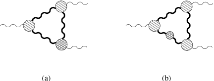
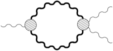
Figure 7: A class of diagrams that can contribute to higher order corrections of the Chern-Simons coefficient in the axial gauge. The hatched vertices and the bold internal lines represent respectively the three point vertices and the propagators which include all the corrections up to $n$-loop order. The cross-hatched vertex and the cross-hatched blob (self-energy) in the internal propagator, include all the corrections up to $(n+1)$-loop order.

Figure 8: Second class of diagrams that can contribute to higher order corrections of the Chern-Simons coefficient in the axial gauge. Here, the diagram involves vertices and propagators of the full theory.

In analyzing the higher loop contributions to the Chern-Simons coefficient, let us note that there are two possible classes of diagrams which are of interest and are shown in Figs. 7 and 8. Let us look at the class of diagrams in Figs. 7a and 7b with all external momenta vanishing. Here the hatched vertices and the bold internal lines represent respectively the three point vertices and the propagators, which include all the corrections up to $n$-loop order, with $n=0,1,2,\cdots$. The cross-hatched vertex, on the other hand, includes all the corrections up to $(n+1)$-loop order, starting from one-loop (namely, it does not contain the tree level term). Similarly, the cross-hatched loop in the internal propagator stands for the self-energy, which includes all the corrections up to $(n+1)$-loops (by definition, the self-energy does not contain the tree level two point function). We will put an overline, on these two factors, just to emphasize that they do not contain the tree level contribution. It is clear now that, by construction, the diagrams in Figs. 7a and 7b lead to contributions only at two loops and higher. Furthermore, from the definition given above, we can write, in the notation described earlier

$$\overline{\Gamma}^{\lambda}=ig\partial^{\lambda}\overline{\Pi}$$ (56)

The contributions from the diagrams in Figs. 7a and 7b, when contracted with $\epsilon_{\mu\nu\lambda}$, would yield a part of the $(n+2)$-loop corrections to the Chern-Simons term and takes the form

$$I^{(n+2)}_{(7a)+(7b)}={\rm Tr}\int d^{3}q\,\epsilon_{\mu\nu\lambda}\left[\left(D\Gamma^{\mu}D\Gamma^{\nu}D\left(\overline{\Gamma}^{\lambda}+\Gamma^{\lambda}D\overline{\Pi}\right)\right)^{(n+1)}+{\rm cyclic}\right]$$

$$=-i\,g^{3}\,{\rm Tr}\int d^{3}q\,\epsilon_{\mu\nu\lambda}\left[\left(\partial^{\mu}D\partial^{\nu}\Pi\left(D\partial^{\lambda}\overline{\Pi}+\partial^{\lambda}D\overline{\Pi}\right)\right)^{(n+1)}+{\rm cyclic}\right]$$

$$=-i\,g^{3}\,{\rm Tr}\int d^{3}q\,\epsilon_{\mu\nu\lambda}\left[\partial^{\lambda}\left(\partial^{\mu}D\partial^{\nu}\Pi D\overline{\Pi}\right)^{(n+1)}+{\rm cyclic}\right]=0$$ (57)

for all $n=0,1,2,\cdots$, where the superscript $(n+1)$ stands for the order of the terms in the expression. Here, “Tr” denotes trace over the matrix indices in the Lorentz space and we have used the identities in Eqs. (54)-(56) in deriving Eq. (57). (There are also matrix indices associated with internal symmetry and these are not traced, but it is clear that they are not relevant for our argument.) We note that, because of the $\epsilon$ tensor, the factor inside the divergence in the integrand picks out only parity violating terms in the amplitude, which converge sufficiently rapidly to zero as $q\rightarrow\infty$. This shows that all the higher loop contributions to the Chern-Simons coefficient, coming from the class of diagrams in Figs. 7a and 7b, vanish.

We can, similarly, show that all the contributions, to the Chern-Simons coefficient, coming from the class of diagrams in Fig. 8 identically vanish. We have already seen it explicitly in our one-loop calculation in the previous section. Here, we show that it is true for this class of diagrams at any loop. Let us note that, from the identities in Eq. (3), we can also express the four point function with two external momenta vanishing, in terms of the three point vertex with one external momentum vanishing in the compact form as (all momenta are incoming)

$$\Gamma^{\nu\lambda}(q,-q;0,0)=ig\left[{\partial\over\partial q_{\lambda}}\Gamma^{\nu}(q,-q^{\prime};q-q^{\prime})\right]_{q^{\prime}=q}\equiv ig\partial^{\lambda}\Gamma^{\nu}$$ (58)

where, again, we have suppressed the internal indices and we follow the convention that the momenta associated with the indices $\nu,\lambda$ of the four point vertex as well as that associated with the index $\nu$ of the three point vertex vanish. Written out explicitly, the right hand side of Eq. (58) would involve two terms with different distributions of the internal symmetry indices, as is clear from Eq. (3). However, as we have emphasized earlier, the internal symmetry factors are not very relevant to the proof of our result.

With these, let us look at the class of graphs in Fig. 8, with all external momenta vanishing. As opposed to the diagrams in Fig. 7a and 7b, here all the vertices and the propagators include corrections to all orders (namely, they are the full vertices and propagators of the theory). With the use of Eqs. (55) and (58), the contraction of $\epsilon_{\mu\nu\lambda}$ with the amplitude in Fig. yields

$$I_{(8)} = {\rm Tr}\int d^{3}q\,\epsilon_{\mu\nu\lambda}D\Gamma^{\mu}D\Gamma^{\nu\lambda}=-g^{2}\,{\rm Tr}\int d^{3}q\,\epsilon_{\mu\nu\lambda}\,\partial^{\mu}D\partial^{\lambda}\Gamma^{\nu}$$ (59)

$$= -g^{2}\,{\rm Tr}\int d^{3}q\,\partial^{\mu}\left(\epsilon_{\mu\nu\lambda}D\partial^{\lambda}\Gamma^{\nu}\right)=0$$

Once again, the integrand in Eq. (59) is sufficiently convergent (because it involves only the parity violating parts of the amplitude) so that the integral vanishes.

Since these are all the diagrams that can contribute to the higher loop corrections of the Chern-Simons coefficient, we have shown that, in a Yang-Mills-Chern-Simons theory, the Chern-Simons coefficient, in the axial gauge, does not receive any correction beyond the one loop order. In other words, much like the proof in the Abelian theory, we have used the non-Abelian Ward identities in the axial gauge, together with the analyticity of the amplitudes in momentum space, to show that the Chern-Simons coefficient has no quantum correction beyond one-loop in this gauge. (We have explicitly checked that, in the axial gauge, the two loop corrections of the Chern-Simons coefficient do add up to zero.) In theories where these assumptions are valid, we will expect our proof to hold true. On the other hand, if either of these assumptions is violated, the proof is expected to break down, which is quite similar to the case in the Abelian theory. Thus, for example, in an Abelian theory with charged massless particles, infrared divergences invalidate the second assumption [18]. Similarly, at finite temperature, it is known that the amplitudes are non-analytic in the energy-momentum variables [10] and, consequently, the Coleman-Hill result is known to be violated in this case [19].

It is worth discussing the implications of this result in some detail. After all, we have already argued, in section 2, that the Chern-Simons coefficient is, in general, gauge dependent. Therefore, even if it has no higher loop corrections in the axial gauge, this may not hold in other gauges. For example, in references [20, 21], the non-abelian Chern-Simons theory was investigated by the use of gauge invariant regularizations in covariant gauges, and was argued that the higher order radiative corrections are finite. Let us note here that (see Eq. (34) and the discussion there), since the Chern-Simons coefficient does not receive any higher loop correction in the axial gauge, it implies that, in this gauge, the ratio ${4\pi m\over g^{2}}$ also does not receive any higher loop correction. On the other hand, as we have argued, this ratio is a gauge independent quantity. Consequently, our result can also be understood as saying that, in any infrared safe gauge, the ratio ${4\pi m\over g^{2}}$ does not receive any contribution beyond one loop. This, in fact, is the appropriate generalization of the Coleman-Hill result to non-Abelian theories. In particular, we note from Eq. (33) that, since in a non-axial type gauge such as the Landau gauge, $Z_{1}\neq Z_{3}$, in such gauges, the Chern-Simons coefficient ($Z_{m}$) will be corrected at higher loops, but in such a way that the ratio ${4\pi m\over g^{2}}$ is unrenormalized beyond one loop.

Such a result has, of course, been expected and predicted [5, 7]. In fact, there is a plausibility argument for this, based on large gauge invariance of the theory in the following way. The only dimensionless ratio, in this theory, is ${g^{2}\over 4\pi m}$ where $4\pi$ is a simple normalization. Therefore, one can use this as a perturbation parameter and write

$$\left({4\pi m\over g^{2}}\right)_{\rm ren}={4\pi m\over g^{2}}\,\sum_{n=0}^{\infty}a_{n}(N)\left({g^{2}\over 4\pi m}\right)^{n}$$ (60)

with $a_{0}(N)=1$ and, as we have seen, $a_{1}(N)=N$. On the other hand, the invariance of the Chern-Simons theory under large gauge transformations requires that this ratio be quantized (see Eq. (5)), both in the bare as well as in the renormalized theory (they don’t have to be the same positive integer). Clearly, this is possible for arbitrary integers and colour factors, only if the series, on the right hand side of Eq. (60) terminates after the second term, namely, only if there is no contribution in Eq. (60) beyond one loop. Our proof explicitly verifies that this expectation is, indeed, true. However, it is important to recognize that our proof uses constraints coming only from the behaviour under small gauge invariance (and, of course, analyticity) much like the proof in the Abelian case. It is worth remarking here that, in a recent paper [22], it has been argued, using a generalization of the method of holomorphy due to Seiberg [23], that in a Yang-Mills theory interacting with matter fields, without a tree level Chern-Simons term, there is no higher loop renormalization of the induced Chern-Simons coefficient. Our result, for the case with a tree level Chern-Simons term, is not covered by this analysis (as the authors of ref. [22] specifically point out) and, in fact, this case is physically more meaningful since, without a tree level Chern-Simons term, a loop expansion of the theory may not exist because of severe infrared divergences. In such a case, general formal arguments may be invalidated by the infrared divergences of the perturbation theory.

6 Pure Chern-Simons theory:

In this section, we will study in detail the pure Chern-Simons theory [24] (otherwise also known as the $\epsilon$-theory [7]) in the infrared safe axial gauge and show that it is a free theory. The pure Chern-Simons theory can be obtained from the Lagrangian density in Eq. (1) (or (2)) by dropping the Yang-Mills term (namely, it is the theory in the $m\rightarrow\infty$ limit). It is well known that, in the Landau gauge, this theory is invariant under a vector supersymmetry [25], in addition to the usual BRST symmetry of Eq. (13). Namely, the Lagrangian density

$${\cal L}={m\over 2}\,\epsilon^{\mu\nu\lambda}A_{\mu}^{a}(\partial_{\nu}A_{\lambda}^{a}+{g\over 3}f^{abc}A_{\nu}^{b}A_{\lambda}^{c})-F^{a}(\partial_{\mu}A^{\mu a})+\partial^{\mu}\overline{c}^{a}(D_{\mu}c^{a})$$ (61)

is, of course, invariant under the BRST transformations of Eq. (13), but it is also invariant under the transformations,

$$\delta A_{\mu}^{a} = \epsilon_{\mu\nu\lambda}\epsilon^{\nu}\partial^{\lambda}c^{a}$$

$$\delta c^{a} = 0$$

$$\delta\overline{c}^{a} = \epsilon^{\mu}A_{\mu}^{a}$$

$$\delta F^{a} = \epsilon^{\mu}(D_{\mu}c^{a})$$ (62)

Here $\epsilon^{\mu}$ is a constant vector parameter of the transformations and is anti-commuting in nature. Furthermore, the generators of these transformations satisfy a supersymmetry algebra, unlike the BRST charges which are nilpotent.

Let us next show that this supersymmetry is not particular to the Landau gauge only. It is easy to see that there is a vector supersymmetry in the axial gauge as well. Thus, the Lagrangian density

$${\cal L}={m\over 2}\,\epsilon^{\mu\nu\lambda}A_{\mu}^{a}(\partial_{\nu}A_{\lambda}^{a}+{g\over 3}f^{abc}A_{\nu}^{b}A_{\lambda}^{c})-F^{a}(n^{\mu}A_{\mu}^{a})-\overline{c}^{a}n^{\mu}(D_{\mu}c^{a})$$ (63)

is invariant under the BRST transformations of Eq. (13) as well as the transformations

$$\delta A_{\mu}^{a} = \epsilon_{\mu\nu\lambda}\epsilon^{\nu}n^{\lambda}c^{a}$$

$$\delta c^{a} = 0$$

$$\delta\overline{c}^{a} = -\epsilon^{\mu}A_{\mu}^{a}$$

$$\delta F^{a} = \epsilon^{\mu}\partial_{\mu}c^{a}$$ (64)

In fact, it is quite easy to check that, in any linear, homogeneous infrared safe gauge, the theory develops an invariance under a vector supersymmetry.

Let us analyze the pure Chern-Simons theory in the axial gauge. In such a case, there is the usual Ward identities following from the BRST invariance of Eq. (13). And, as we have noted earlier, the structure of the theory leads to the fact that, in the axial gauge, there is no wave function or vertex renormalization for the ghosts. Let us note now that the new vector supersymmetry will also lead to a Ward identity, further restricting the amplitudes. The master identity, following from the invariance of the theory under Eq. (64) takes the form (We note here that the derivation of this identity is much simpler than the usual Ward identities because the transformations in Eq. (64) are, in fact, linear and, consequently, we do not need additional sources in the Lagrangian density.)

$$\int d^{3}x\left(\epsilon_{\mu\nu\lambda}\,{\delta\Gamma\over\delta A_{\nu}^{a}(x)}c^{a}(x)n^{\lambda}-{\delta\Gamma\over\delta F^{a}(x)}\partial_{\mu}c^{a}(x)+A_{\mu}^{a}(x){\delta\Gamma\over\delta\overline{c}^{a}(x)}\right)=0$$ (65)

This, indeed, constrains the theory enormously. Combining with the facts that the $F^{a}A_{\mu}^{a}$ vertex, the ghost two point vertex and the ghost interaction vertices are not renormalized, it immediately leads us to the result that the two point and the three point functions for the gauge fields are not renormalized either. For example, taking derivative of Eq. (65) with respect to ${\delta^{2}\over\delta A_{\mu}^{a}\delta c^{b}}$ (index $\mu$ being summed) and setting all fields to zero, we obtain in momentum space

$$\epsilon_{\mu\nu\lambda}n^{\lambda}{\delta^{2}\Gamma\over\delta A_{\mu}^{a}(-p)\delta A_{\nu}^{b}(p)}+ip_{\mu}{\delta^{2}\Gamma\over\delta A_{\mu}^{a}(-p)\delta F^{b}(p)}-3{\delta^{2}\Gamma\over\delta\overline{c}^{a}(-p)\delta c^{b}(p)}=0$$ (66)

This immediately leads to $Z_{m}=1$. Similarly, taking one higher derivative, it is easy to show that the parity violating three point vertex function is not renormalized either. In other words, the pure Chern-Simons theory is a free theory. These conclusions are valid provided one regularizes the theory such that all symmetries, including the vector supersymmetry, are maintained. We would like to note here that such a conclusion was reached earlier from different points of view [7, 26, 27, 28]. In particular, in reference [26], it was shown through a perturbative calculation in the pure Chern-Simons theory, that the complete effective action in axial gauges is the three level action, for certain classes of gauge invariant regulators. Here we have derived this result from purely algebraic considerations.

7 Conclusion:

In this paper, we have studied in detail the question of higher order corrections to the Chern-Simons coefficient in a Yang-Mills-Chern-Simons theory. We have shown that the Chern-Simons coefficient is, in general, a gauge dependent quantity. However, it takes on a physical significance in the axial gauge. Using, i) the Ward identities of the theory and, ii) the analyticity of the amplitudes in the momentum variables, we have shown that, in the axial gauge, the Chern-Simons coefficient does not receive any quantum correction beyond one loop. This allows us to deduce that the ratio ${4\pi m\over g^{2}}$, in a non-Abelian theory, is not renormalized beyond one loop, in any infrared safe gauge. This, therefore, represents the generalization of the Coleman-Hill result to a non-Abelian theory. Various other interesting properties of the theory are also discussed.

This work was supported in part by U.S. Dept. Energy Grant DE-FG 02-91ER40685 as well as by CNPq, Brazil.

References

- [1] S. S. Chern and J. Simons, Ann. Math. 99 (1974) 48.
- [2] S. Deser, R. Jackiw and S. Templeton, Phys. Rev. Lett. 48(1982) 975; Ann. Phys. 140 (1982) 372.
- [3] R. Jackiw and S. Templeton, Phys. Rev. D23 (1981) 2291.
- [4] M. D. Bernstein and T. Lee, Phys. Rev. D32, (1985) 1020.
- [5] Y.-C. Kao and M. Suzuki, Phys. Rev. D31, (1985) 2137.
- [6] S. Coleman and B. Hill, Phys. Lett. B159 (1985) 184.
- [7] R. D. Pisarski and S. Rao, Phys. Rev. D32 (1985) 2081.
- [8] F. T. Brandt, A. Das, and J. Frenkel, Phys. Lett. B494, (2000) 339.
- [9] N. K. Nielsen, Nucl. Phys. B101 (1975) 173.
- [10] A. Das, Finite Temperature Field Theory, World Scientific (1997).
- [11] A. N. Redlich, Phys. Rev. D29 (1984) 2366.
- [12] K. S. Babu, A. Das, and P. Panigrahi, Phys. Rev. D36 (1987) 3725.
- [13] G. V. Dunne, Lectures given at Les Houches Summer School in Theoretical Physics, Session 69: Topological Aspects of Low-dimensional Systems, Les Houches, France, 7-31 Jul 1998. hep-th/9902115.
-
[14]
W. Kummer, Acta Phys. Austriaca 14 (1961)
149; ibid 41 (1975) 315;
R. L. Arnowitt and S. Fickler, Phys. Rev. 127 (1962) 1821;
J. Frenkel, Phys. Rev. D13 (1976) 2325;
G. Leibbrandt, Rev. Mod. Phys. 59 (1987) 1067. -
[15]
E. Witten Comm. Math. Phys. 121 (1989) 351;
S. Elitzur, G. Moore, A. Schwimmer and N. Seiberg, Nucl. Phys. 326 (1989) 108;
M. Bos and V. P. Nair, Int. J. Mod. Phys. A5 (1990) 959;
M. Bos and V. P. Nair, Phys. Lett. B223 (1989) 61;
J. M. F. Labastida and A. V. Ramallo, Phys. Lett. B227 (1989) 92. - [16] A. Polyakov, Fields, Strings and Critical Phenomena, Les Houches, eds. E. Brézin and J. Zinn-Justin (1988).
- [17] K. Gawedzki and A. Kupiainen, Nucl. Phys. B320 (1989) 625.
- [18] G. Semenoff, P. Sodano and Y.-S. Wu, Phys. Rev. Lett. 62 (1989) 715.
- [19] F. T. Brandt, Ashok Das, J. Frenkel and K. Rao, Phys.Lett. B492 (2000) 393.
- [20] E. Guadagnini, M. Martellini and M. Mintchev, Phys. Lett. B227 (1989) 111.
- [21] J. M. F. Labastida and A. V. Ramallo, Nucl. Phys. B334 (1990) 103.
- [22] M. Sakamoto and H. Yamashita, Phys. Lett. B476 (2000) 427.
- [23] N. Seiberg, Phys. Lett. B318 (1993) 469.
- [24] C. R. Hagen, Phys. Rev. D31 (1985) 331.
- [25] D. Birmingham, M. Blau, M. Rakowski and G. Thompson, Phys. Rep. 209 (1991) 129. This is a good source for other references as well as information on other aspects of topological theories.
- [26] C. P. Martin, Phys. Lett. B263 (1991) 69.
- [27] G. Leibbrandt and C.P. Martin, Nucl. Phys. B416 (1994) 351.
-
[28]
A. Brandhuber, S. Emery, M. Langer, O. Piguet, M. Schweda and
S.P. Sorella, Helv. Phys. Acta 66 (1993) 551;
S. Emery and O. Piguet, Helv. Phys. Acta 67 (1994) 22;
For observations on BF theories as well as other references, see, O. Piguet, “Ultraviolet properties of topological gauge theories”, talk at the “Second International School on Field Theory and Gravitation”, Vitória, to be published.