SU-ITP 00-32

RU-NHETC-2000-46

hep-th/0012065

Gauge Invariant Correlators in

Non-Commutative Gauge Theory

Moshe Rozali^a and Mark Van Raamsdonk^b

^a Department of Physics and Astronomy

Rutgers University

Piscataway, NJ 08855

rozali@physics.rutgers.edu

^b Department of Physics

Stanford University

Stanford, CA 94305 U.S.A.

mav@itp.stanford.edu

Abstract

Using perturbation theory, we explore the universal high momentum behavior of correlation functions of gauge invariant operators in planar noncommutative gauge theories. We find that the correlation functions are strongly enhanced when pairs of momenta become antiparallel. In particular, there is a transition from the previously noted exponential suppression of correlation functions at high momenta to a more field theoretic behavior when the momenta of pairs of operators antialign within a critical angle. Some of our calculations can be extrapolated to strong coupling, and in particular we are able to reproduce precisely the supergravity prediction for the behavior of two point functions, including the coupling dependence.

1 Introduction

Many of the recent interesting developments in string theory have centered around various non-gravitational theories that arise from string theory in “decoupling” limits. These include local quantum field theories, such as the ${\cal N}=4$ SYM theory, plus non-local theories without a known explicit description, such as little string theories. Somewhere in between are the non-commutative field theories which arise in certain decoupling limits involving D-branes with NS-NS two-form fields turned on in their worldvolume directions [1, 2, 3, 4]. These theories are non-local, yet possess explicit Lagrangian descriptions in the language of ordinary quantum field theory that allow perturbative calculations.

Perturbative analysis of noncommutative field theories has revealed many interesting properties (see e.g. [5, 6]). In particular, the theories display a mixing of the infrared and the ultraviolet: short distance physics can lead to significant long range effects. From a technical point of view, these effects arise from internal momentum dependent phase factors which appear in non-planar graphs of the theory. On the other hand, planar graphs behave identically to their counterparts in the commutative theory apart from overall external momentum dependent phase factors. One might then expect that large N noncommutative field theories should have basically the same behavior as their commutative counterparts, since non-planar diagrams are suppressed by powers of ${1\over N}$. However, it turns out that at least for noncommutative gauge theories, the commutative and noncommutative versions have very different behavior at large momenta, even in the planar, large $N$ limit.

This differing behavior can be seen easily for the particular case of ${\cal N}=4$ SYM theory by comparing the conjectured supergravity duals for the two cases. In the commutative case, the corresponding gravitational theory is of course type IIB string theory on $AdS^{5}\times S^{5}$ which arises as the near horizon geometry of a stack of D3-branes [7]. In the noncommutative case, the dual theory is type IIB string theory in a background which has been worked out in [8, 9]. The two solutions have identical behavior in the “infrared” part of the space (near $r=0$), suggesting that the two field theories are equivalent at low energies. On the other hand, the supergravity dual of the noncommutative theory has an Einstein frame metric [10] which is asymptotically flat in the $r\to\infty$ region (though the coupling goes to zero here) in sharp contrast with the asymptotically AdS dual of the commutative theory. Thus, we expect that the UV behavior of noncommutative ${\cal N}=4$ SYM theory differs significantly from the behavior of its commutative counterpart, even for large $N$. The different behavior in the ultraviolet reflects the fact that unlike conventional field theories, non-commuatative gauge theories are not defined by a UV fixed point [11]. It seems particularly interesting to understand this UV behavior, since it provides the field theory dual of gravity on a space which is not asymptotically AdS.

In this paper, we study the high momentum behavior of correlation functions of gauge invariant operators in noncommutative gauge theory. As discussed in [12]-[18] and reviewed in section 2 of this paper, these operators involve open Wilson lines which extend in the directions perpendicular to the operator momentum with a length proportional to the momentum. This transverse spreading at high momenta is in accord with the uncertainty relation associated with the commutation relations for the coordinates, $[x^{\mu},x^{\nu}]=i\theta^{\mu\nu}$. The extended nature of the gauge invariant operators leads to qualitatively different behavior of high momentum correlation functions as compared with the commutative theory.

In [16], the two point functions of these operators were calculated at weak coupling and shown to have a universal exponential behavior with high momentum,

$$\langle O(k)O(-k)\rangle\sim{\rm exp}\left(\sqrt{{g^{2}N|k||k\theta|\over 4\pi}}+\dots\right)$$ (1)

where the dots indicate a regularization dependent term that cancels out in properly normalized correlation functions. The authors showed that the momentum dependence of this expression is identical to that of the two point function calculated using the supergravity dual of noncommutative ${\cal N}=4$ SYM theory, though the supergravity result has a different coupling dependence, obtained by the replacement $g^{2}N\to\sqrt{g^{2}N}$ in (1). In this paper, we show that even this coupling dependence can be reproduced by a perturbative field theory calculation extrapolated to strong coupling. We describe this result in section 4 and offer two possible explanations for the agreement.

In the rest of the paper we consider the high momentum behavior of more general correlation functions. We find a rather universal effect: the correlation functions are very sharply enhanced when the momenta of pairs of operators becomes antiparallel. In particular, for a pair of operators with large nearly antiparallel large momenta of order $k$, ($|k||\theta k|\gg 1$) we find that the correlation functions vanish rapidly when the angle between the momenta rises above some critical value, $\phi>{1\over|k||\theta k|}$. As a result of this enhancement amplitudes fall off exponentially with the momenta for generic angles, but cross-over to a more field theoretic behavior below this critical small angle.

The structure of the paper is as follows. In section 2, we review the construction of gauge invariant operators in noncommutative gauge theories and discuss in particular the operators corresponding to supergravity modes in the gauge theory - gravity correspondence for ${\cal N}=4$ SYM theory. In section 3, we provide a general formula for computing planar correlation functions of operators involving open Wilson lines. In section 4, we discuss the calculation of two-point functions and in section 5 we extend this discussion to higher point functions. We offer some comments and a summary of the results in section 6.

2 Gauge Invariant Operators

In this section, we review the construction of gauge invariant operators in noncommutative gauge theories as well as the specific form of operators corresponding to bulk supergravity modes in the gauge theory - gravity correspondence for noncommutative ${\cal N}=4$ SYM theory.

To begin, we recall the transformation properties of the gauge field in noncommutative gauge theory,

$$A_{\mu}\rightarrow U(x)\star A_{\mu}\star U(x)^{\dagger}-{i\over g}U(x)\star\partial_{\mu}U^{\dagger}(x)$$ (2)

We will take a $U(N)$ gauge group, so that $A_{\mu}$ is an $N\times N$ hermitian matrix. The gauge covariant field strength is then given by

$$F_{\mu\nu}=\partial_{\mu}A_{\nu}-\partial_{\nu}A_{\mu}+ig(A_{\mu}\star A_{\nu}-A_{\nu}\star A_{\mu})$$ (3)

and the (Euclidean) gauge invariant action for the gauge fields is

$$S={1\over 4}\int d^{4}x{\rm Tr}\ (F_{\mu\nu}\star F_{\mu\nu})$$ (4)

(equivalently, the star product may be replaced by an ordinary product). In more general theories such as the ${\cal N}=4$ SYM theory, we may have additional matter fields, but the generalization of the action to a noncommutative theory is always obtained by replacing products by star products.

We now turn to the construction of gauge invariant operators. A remarkable property of noncommutative gauge theories (with all fields transforming in the adjoint) is that translations in the noncommutative directions are gauge transformations,

$$f(x^{\mu}+\theta^{\mu\nu}k_{\nu})=e^{ik\cdot x}\star f(x^{\mu})\star e^{-ik\cdot x}$$ (5)

As a result, it is impossible to construct local gauge invariant operators. On the other hand, it is possible to construct gauge invariant operators that are local in momentum space, as shown in [12, 16, 17, 18].

The construction employs open Wilson lines, defined by

$$W(x,C) = {\rm Tr}\ \left({\rm P}_{\star}e^{ig\int_{C}A_{\mu}dx^{\mu}}\right)$$

$$= \sum_{n=0}^{\infty}(ig)^{n}\int_{0}^{1}d\sigma_{1}\cdots\int_{\sigma_{n-1}}^{1}d\sigma_{n}\dot{\zeta^{\mu_{1}}}\cdots\dot{\zeta^{\mu_{n}}}$$

$$\hskip 93.95122pt{\rm Tr}\ \left(A_{\mu_{1}}(x+\zeta(\sigma_{1}))\star\cdots\star A_{\mu_{n}}(x+\zeta(\sigma_{n}))\right)$$

where $P_{\star}$ denotes path ordering and $C$ is a path parameterized by $\zeta(\sigma)$ with $\zeta(0)=x$. These transform covariantly under gauge transformations,

$$W(x,C)\rightarrow U(x)\star W(x,C)\star U^{\dagger}(x+\zeta(1))$$ (7)

Now, given a set of gauge covariant local operators $\{{\cal O}_{i}\}$ transforming in the adjoint, we may construct a gauge invariant operator local in momentum space by taking

$$\hat{\cal O}(k)=\int e^{ik\cdot x}{\rm Tr}\ ({\cal O}_{1}(x)\star W(x,C_{1})\star{\cal O}_{2}(x+l_{1})\star\cdots\star W(x+l_{1}+\dots+l_{n-1},C_{n}))$$ (8)

where $l_{i}=\zeta_{i}(1)$. Using the relation (5), it is simple to show that this operator is gauge invariant provided that

$$l^{\mu}_{1}+\dots+l^{\mu}_{n}=\theta^{\mu\nu}k_{\nu}$$ (9)

This operator is precisely the result of taking insertions of any set of local covariant operators at arbitrary point on an open Wilson line whose endpoints are separated by $\tilde{k}\equiv\theta^{\mu\nu}k_{\nu}$, as diagrammed in figure 1.

Figure 1: A general Wilson line operator with momentum $k$.

In fact, it is somewhat misleading to refer to these objects as open Wilson lines, as the endpoints of the interval are not distinguished. Noting that

$$\int e^{ik\cdot x}\,{\rm Tr}\ ({\cal O}_{1}(x)\star W(x,C)\star{\cal O}_{2}(x+\tilde{k}))=\int e^{ik\cdot x}\,{\rm Tr}\ ({\cal O}_{2}(x)\star{\cal O}_{1}(x)\star W(x,C))\;,$$ (10)

we see that the operators at each end of the open Wilson line may equivalently be taken at a single point by a cyclic rearrangement.

For the case of noncommutative ${\cal N}=4$ SYM theory, there is now compelling evidence [16, 22, 23] that the operators corresponding to particle states in the dual gravitational theory are gauge invariant operators whose form is a special case of the construction described so far. Recall that for the usual commutative ${\cal N}=4$ theory, operators corresponding to particles in $AdS^{5}\times S^{5}$ are chiral operators which take the form of a symmetrized trace of a product of gauge covariant objects (scalars, fermions, field strengths, or covariant derivatives of these),

$${\cal O}(k)=\int e^{ik\cdot x}\,{\rm STr}\ (B_{1}\cdots B_{n})(x)$$ (11)

It turns out that the appropriate generalization of this operator to the noncommutative theory is given by

$${\cal O}(k)=\int e^{ik\cdot x}\,{\rm\hat{STr}}(B_{1}\star\cdots\star B_{n}\star W(x,\tilde{k}))$$ (12)

where $W(x,\tilde{k})$ is a Wilson line with a straight line path from $x$ to $x+\tilde{k}$ and ${\rm\hat{STr}}$ denotes that the expression is to be averaged over all ways of inserting the $B$s into separate points on the the Wilson line. Thus, the individual factors in the product become spread out linearly over a transverse distance $\tilde{k}$.

In the following sections we study general correlation functions of these straight Wilson line operators, in particular looking for universal behavior at high momenta that arises from the extended nature of the operators. It is interesting to note that due to the asymptotically flat nature of the supergravity dual (in the maximally supersymmetric case), there are scattering states in the dual geometry, and it is likely that the correlations functions we compute correspond to S-matrix elements of these scattering states. This is similar to the situation in linear dilaton backgrounds [24], and is in contrast to the asymptotically AdS geometries.

3 Correlation Functions of Gauge Invariant Operators

We have seen that the gauge invariant operators in noncommutative gauge theories have an extended structure that differs significantly from the corresponding operators in the commutative theory at high momenta. In this section, we investigate the effects of this extended structure on general correlation functions.

Since we are mainly interested in the effects of the Wilson line part of the operators, we focus on the simple case of Wilson lines with a single insertion of a gauge covariant operator ${\cal O}$. We define

$$W(k) = \int d^{4}x\;e^{ik\cdot x}\star{\rm Tr}\left({\cal O}(x)\star{\rm P}_{\star}e^{ig\int A_{\mu}dx^{\mu}}\right)$$ (13)

$$= \sum_{n=0}^{\infty}(ig)^{n}\int d^{4}x\;e^{ik\cdot x}\int_{0\leq\sigma_{1}\leq\cdots\leq\sigma_{n}\leq 1}\dot{\zeta}^{\mu_{1}}(\sigma_{1})\cdots\dot{\zeta}^{\mu_{n}}(\sigma_{n})$$

$$\hskip 36.135pt{\rm Tr}\left({\cal O}(x)\star A_{\mu_{1}}(x+\zeta(\sigma_{1}))\star\cdots\star A_{\mu_{n}}(x+\zeta(\sigma_{n}))\right)$$

As before, ${\rm P}_{\star}$ denotes noncommutative path ordering, and the Wilson line runs over a path $x^{\mu}=\zeta^{\mu}(\sigma)$ , with $\zeta^{\mu}(1)-\zeta^{\mu}(0)=\tilde{k}^{\mu}\equiv\Theta^{\mu\nu}k_{\nu}$. We will mainly consider the case of a straight Wilson line for which $\zeta^{\mu}(\sigma)=\tilde{k}^{\mu}\sigma$.

We focus on the large $N$ theory, for which planar diagrams are dominant. For such diagrams, the star products appearing in the expansion (13) only have the effect of providing an overall phase factor for the correlation function, which depends on the ordering of the external momenta.

To focus on the UV behavior of the theory, we assume that the external momenta are asymptotically large. More precisely, we assume that the dimensionless quantity $|k||\tilde{k}|$ is large. The amplitudes are then dominated at each order in the ’t Hooft coupling by ladder diagrams, as discussed in [16]. These are diagrams, such as the one shown in figure 2, in which the gauge fields are contracted between various Wilson lines, with no internal vertices. Since we also work at leading order in the ’t Hooft $\frac{1}{N}$ expansion, we are further restricted to planar ladder diagrams.

Figure 2: A typical planar ladder diagram in the correlation function of four Wilson line operators

For planar diagrams in which the Wilson line gauge fields contract only with each other, it is straightforward write down a general expression for the correlation function. We find

$$\langle W(k_{1})\cdots W(k_{n})\rangle_{\rm ladder} = \sum e^{i\sum_{i<j}k_{i}\times k_{j}}\int d^{4}x_{i}\;e^{ik_{i}\cdot x_{i}}\langle{\cal O}_{1}(x_{1})\cdots{\cal O}_{n}(x_{n})\rangle$$ (14)

$$\hskip 43.36243pt\times\int d\vec{\sigma}\prod{g^{2}N\over 4\pi^{2}}{-\dot{\zeta}\cdot\dot{\hat{\zeta}}\over(x-\hat{x})^{2}}$$

Here, the first sum is over all ways of contracting the $A$s between the various Wilson lines to give a planar diagram. The phase factor comes from the star products, but depends only on the ordering of external momenta since the diagrams are planar. In the second line, the integral runs over positions of the $A$s on the various lines (i.e. the endpoints of the propagators), and the product is over all propagators in the diagram. In the integrand, $x$ and $\hat{x}$ represent the two endpoints of a given propagator, while $\zeta$ and $\hat{\zeta}$ are tangent vectors evaluated at $x$ and $\hat{x}$ respectively. A typical diagram in the sum is shown in figure 2.

4 Two Point Functions

We start by calculating two point functions of the gauge invariant operators (13). The calculation was performed previously for weak coupling in [16]. Here, we note that within the approximation of summing only over ladder diagrams, the result may also be evaluated at strong coupling. We find that this strong coupling result exactly reproduces the behavior of the supergravity result including the coupling dependence. At the end of this section we offer two possible explanations for the agreement. A similar result was obtained in [20] in the context of Wilson line correlators for the commutative ${\cal N}=4$ theory, see also [21].

For the two point functions, factoring out the $\delta$-function of momentum conservation, the general formula (14) becomes

$$\left<W(k)W^{\dagger}(k)\right>=\int d^{4}\Delta\,e^{ik\cdot\Delta}f(\Delta)\sum_{n}(\lambda\tilde{k}^{2})^{n}\prod_{i=1}^{n}\int d\tau_{i}\int d\sigma_{i}\,\frac{1}{|\Delta+\tilde{k}(\tau_{i}-\sigma_{i})|^{2}}$$ (15)

Here $\lambda={g^{2}N\over 4\pi^{2}}$, $\Delta=x_{1}-x_{2}$ is the relative position of the operators, and we define

$$\left<O_{1}(x_{1})O_{2}(x_{2})\right>=f(x_{1}-x_{2})\;.$$ (16)

Because of the restriction to planar ladder diagrams, the integrals over $\sigma$ and $\tau$ (which describe the endpoints of the various rungs) are ordered, $0\leq\sigma_{1}\leq\cdots\leq\sigma_{n}\leq 1$, $0\leq\tau_{1}\leq\cdots\leq\tau_{n}\leq 1$. In order to extract the universal large momentum behavior arising from the Wilson lines, we follow [16] and set $f(\Delta)=1$.

The integrand $\frac{1}{|\Delta+\tilde{k}(\tau_{i}-\sigma_{i})|^{2}}$ is a steep function (for large $|\tilde{k}|$) which is maximized at:

$$\tau_{i}-\sigma_{i}=-\frac{\Delta_{\parallel}}{|\tilde{k}|}$$ (17)

where $\Delta_{\parallel}$ is the component of $\Delta$ parallel to $\tilde{k}$. In order to attain this maximum within the integration region one requires:

$$0\leq\Delta_{\parallel}\leq|\tilde{k}|$$ (18)

Since the integrand is steep, we would like to evaluate it using a saddle point approximation starting with the $\tau_{i}$ integrals. However, due to the ordering of the points, $\tau_{i}\leq\tau_{i+1}$, the peak of the integrand may be close to the edges of the integration regime, so the saddle point approximation is not automatically justified. The required condition is that the width of the integrand as a function of a given $\tau_{i}$,

$$\frac{|\Delta_{\perp}|}{|\tilde{k}|}$$

is less than the average spacing between the $\tau_{i}$’s, ${1\over n}$. Thus, to use the saddle point approximation, we need

$$\eta\equiv\frac{n|\Delta_{\perp}|}{|\tilde{k}|}\leq 1$$ (19)

When this condition is satisfied, defining

$$I_{n}=\prod_{i=1}^{n}\int d\tau_{i}\int d\sigma_{i}\frac{\lambda\tilde{k}^{2}}{|\Delta+\tilde{k}(\tau_{i}-\sigma_{i})|^{2}}\;,$$ (20)

we find (first evaluating the $\tau$ integrals using saddle point and then performing the $\sigma$ integrals directly),

$$I_{n}\sim\frac{\lambda^{n}}{n!}\,\frac{\tilde{k}^{n}}{|\Delta_{\perp}|^{n}}$$ (21)

To see that this estimate cannot hold when $\eta\geq 1$, note that the integral $I_{n}$ is bounded from above by the maximum value of the integrand times the volume of the integration region

$$I_{n}\leq\frac{\lambda^{n}}{(n!)^{2}}\,\frac{\tilde{k}^{2n}}{\Delta_{\perp}^{2n}}$$ (22)

It is easy to see that the saddle point result (21) exceeds this bound when $\eta>1$. In fact, the upper bound (22) provides a good approximation to $I_{n}$ for $\eta\geq 1$ (we will show this explicitly in section 5 using a lower bound on $I_{n}$).

In either regime, the integral over $\Delta_{\parallel}$ (which we restrict to the range (18)) can be readily performed, remembering that $k_{\parallel}=0$. Suppressing the subscript of $\Delta_{\perp}$, we get:

$$\left<W(k)W^{\dagger}(k)\right>\simeq|\tilde{k}|\int d^{3}\Delta\,e^{ik\cdot\Delta}\sum_{n}(\frac{\lambda\tilde{k}^{2}}{4\pi})^{n}I_{n}$$ (23)

where

$$I_{n}\sim\left\{\begin{array}[]{ll}{\lambda^{n}\over n!}\left({\tilde{k}\over\Delta}\right)^{n}&\qquad\qquad{n\Delta\over\tilde{k}}<1\\ {\lambda^{n}\over(n!)^{2}}\left({\tilde{k}\over\Delta}\right)^{2n}&\qquad\qquad{n\Delta\over\tilde{k}}>1\end{array}\right.$$ (24)

The correct estimate for $I_{n}$ depends now on the values of $\Delta,n$ dominating the expression for the two-point function. For both estimates of $I_{n}$, the integration over $\Delta$ is dominated by the regime $|\Delta|\simeq\frac{n}{|k|}$, therefore one has $\eta\simeq\frac{n^{2}}{|k||\tilde{k}|}$ in the relevant region of integration. Thus, for $n<\sqrt{k\tilde{k}}$ we may use the $\eta<1$ estimate when integrating over $\Delta$, while for $n>\sqrt{k\tilde{k}}$, we should use the $\eta>1$ estimate.

As explained in [16], we should extract the contribution which is non-analytic in $k$ for each $n$, since the analytic parts correspond to contact terms in position space. The results for the relevant Fourier transforms can be found in [16]. We are left with a sum of terms $\sum_{n}J_{n}$ where the $n$ dependence of $J_{n}$ is given by

$$J_{n}\sim\left\{\begin{array}[]{ll}{\lambda^{n}(k\tilde{k})^{n}\over(n!)^{2}}&\qquad\qquad n<\sqrt{k\tilde{k}}\\ {\lambda^{n}(k\tilde{k})^{2n}\over(n!)^{2}(2n)!}&\qquad\qquad n>\sqrt{k\tilde{k}}\end{array}\right.$$ (25)

For each value of the parameters, the terms in this series will increase to a maximum value at some $n=M$ and then decrease, with the terms for $n\gg M$ giving negligible contribution. At weak coupling, we find that $M\ll\sqrt{k\tilde{k}}$ so only the small $n$ form of $J_{n}$ is relevant. Performing the sum using the small $n$ estimate, we recover precisely the result (1) of [16].

On the other hand, at strong coupling, $M\gg\sqrt{k\tilde{k}}$ so the series is dominated by terms of the large $n$ form. Summing the series in this case, we find (ignoring prefactors)

$$\left<W(k)W^{\dagger}(k)\right>\sim\exp(\sqrt{\sqrt{\lambda}|\tilde{k}||k|})$$ (26)

We note that up to numerical factors (which we have not been careful about), this result is precisely equal to the supergravity result [16] including the coupling dependence.

We offer two possible explanations for this agreement. Firstly, in the case of chiral operators for the ${\cal N}=4$ theory, it is reasonable to guess that two point functions should obey a non-renormalization theorem such that the leading perturbative result is valid at all values of the coupling. But in our case, the leading perturbative result is precisely this sum over ladder diagrams. The higher order ladder diagrams are not perturbative corrections but actually the leading contribution to the correlation function from the higher order terms in the expansion of the operators (13). Thus, assuming a nonrenormalization theorem, we would expect that the sum over ladder diagrams at strong coupling should reproduce the supergravity answer. This is exactly what we find, so our result may be interpreted as providing evidence for this nonrenormalization theorem.

A second possibility for the agreement is that as noted earlier, at high momenta the ladder diagrams give the leading contribution order by order in the ’t Hooft coupling, while diagrams with internal vertices are suppressed by inverse powers of momenta. It is therefore possible that in the large momentum limit, the restriction to a sum over ladder diagrams is sensible even at strong coupling, providing another possible explanation of the agreement we find. If this is the case, it would indicate that both chiral and nonchiral operators in the theory share this universal behavior at large momenta. From the supergravity point of view, this would indicate a similar behavior in the UV region for both supergravity modes and stringy modes.

5 Higher Point Functions

We turn now to higher point functions of the noncommutative operators. We will show that for large momenta, the correlation functions are sharply peaked, preferring the kinematics in which pairs of momenta are antiparallel. The properly normalized correlation functions generically exhibit exponential decay at large momenta, as described in [16]. However, at small enough angles we find that the amplitudes are enhanced, and the dependence on momenta has a cross-over to a more typical field theoretic behavior, as described below.

We consider then the correlation functions $\langle W_{1}(k_{1})W_{2}(k_{2})\cdots W_{n}(k_{n})\rangle$. In the limit of large $k_{i}$ in the sense described above, we will show that ladder diagrams must generally be included even at weak coupling, as was the case for the two point functions. As we have discussed, the ladder diagrams dominate any diagrams with internal vertices at each order in the ’t Hooft coupling. Diagrams with internal vertices are suppressed by powers of ${1\over|k||\tilde{k}|}$, so working in the order of limits in which the momenta are taken large first, we may consider only the ladder diagrams. These may be summed explicitly both for weak and strong coupling, and we provide the results for both cases. We emphasise that summing over ladder diagrams at strong coupling can be justified only with our carefully chosen order of limits. The agreement with the gravity results for the two-point function is an indication that the sum over ladder diagrams may be sensible even in the limit of strong coupling.

In subsection 5.1 we derive the conditions under which it is necessary to include ladder diagrams connecting a given pair of operators $W_{1},W_{2}$. We will see that in a weak coupling calculation and for generic angles between the momenta $\tilde{k_{i}}$, there is no need to include ladder diagrams, and we may use the leading perturbative result. However, when two momenta $\tilde{k_{1}},\tilde{k_{2}}$ are nearly anti-parallel, the sum over ladders connecting $W_{1},W_{2}$ is necessary, and provides an enhancement of the amplitude. At strong coupling, ladder diagrams will be important for all angles.

In section 5.2 we present the approximation schemes which are appropriate for evaluation of this universal behavior in both the weak and strong coupling regimes. These approximation schemes generalize the two estimates ($\eta<1$ and $\eta>1$) for the two point functions, presented in the previous section. In the sections 5.3 and 5.4, we perform the calculation of the ladder diagram contributions in each of these regimes.

The reader interested only in the results of the calculation is invited to skip to section 6, where our results are summarized and discussed.

5.1 Conditions for Including Ladder Diagrams

Given a general correlation function, we would first like to determine the conditions under which it is necessary to include ladder diagrams connecting a pair of operators $W_{1}(k)$ and $W_{2}(-l)$ in a perturbative calculation. We will find that ladder diagrams dominate the leading order perturbative result when the angle between $\tilde{k}$ and $\tilde{l}$ is less than a particular upper bound.

To begin, consider a diagram involving an additional contraction between gauge fields in the Wilson lines associated with $W_{1}$ and $W_{2}$. Relative to the leading order perturbative result (with no contractions between the Wilson lines) this diagram will have an additional factor of

$$\lambda(\tilde{k}\cdot\tilde{l})\,\int_{0}^{1}d\sigma\int_{0}^{1}d\tau{1\over(\Delta+\tilde{k}\sigma-\tilde{l}\tau)^{2}}$$ (27)

We wish to determine when this factor is of order 1 or larger, in which case the diagram (and higher order ladder diagrams) must be included.

For simplicity, we assume that $\Delta$ is perpendicular to $\tilde{k}$ and $\tilde{l}$, which are taken to have the same magnitude. In this case, the integral may be evaluated explicitly, and the relative factor becomes

$$\lambda\cot(\phi)\sinh^{-1}\left({\tilde{k}\sin{\phi\over 2}\over\Delta}\right)\;,$$ (28)

where $\phi$ denotes the angle between $\tilde{k}$ and $\tilde{l}$, assumed to be small. The distance $\Delta$ lies purely in the commutative directions.

The typical value of $\Delta$ for operators of momentum $k$ will be roughly $\Delta={1\over|k|}$, so we estimate that the ladder diagram contributions will be important for

$${\lambda\over\phi}\sinh^{-1}(|k||\tilde{k}|\phi)>1$$ (29)

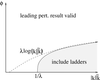
Figure 3: Angles and momenta for which ladder diagrams dominate the leading perturbative result.

This region is diagrammed in figure 3. We see that ladder diagrams must be included for small angles whenever $|k||\tilde{k}|\geq 1/\lambda$. In particular, for momenta such that $|k||\tilde{k}|\gg 1/\lambda$, ladder diagrams must be included when

$$\phi<\lambda\log(|k||\tilde{k}|)\;.$$ (30)

At larger angles, the ladder diagrams do not make a significant contribution, and we can trust the leading order perturbative result. At weak coupling, this cutoff angle remains small ($\ll 1$) as long as $|k||\tilde{k}|<e^{1\over\lambda}$, so the leading order perturbative result is fine for generic angles $(\phi\sim 1)$. On the other hand, it is obvious that ladder diagrams will dominate the leading perturbative result at strong coupling for any angles.

5.2 Approximation Schemes

We would like to calculate the contribution to the correlation function

$$\langle W_{1}(k)W_{2}(-l)\cdots W_{n}\rangle$$ (31)

from the sum over ladders connecting the Wilson lines in $W_{1},W_{2}$ in the case where $k$ and $-l$ are very large and nearly antiparallel. We are interested in universal behavior arising from the extended nature of the Wilson lines, independent of the details of the operators $W_{i}$.

From the general formula (14), we see that the correlation function has the following dependence on $k,l$

$$\langle W_{1}(k)W_{2}(-l)\cdots W_{n}\rangle\sim\int d^{4}\Delta\exp(i\Delta\cdot(k-l)/2)f(\Delta,\cdots)\sum_{n}{\cal I}_{n}$$ (32)

where $f$ represents the commutative position space correlator, and ${\cal I}_{n}$ is the contribution coming from the ladder diagram with $n$ rungs connecting $W_{1}$ and $W_{2}$ (see figure 4),

$${\cal I}_{n}=\int_{0}^{1}d\sigma_{n}\cdots\int_{0}^{\sigma_{2}}d\sigma_{1}\;\int_{0}^{1}d\tau_{n}\cdots\int_{0}^{\tau_{2}}d\tau_{1}\;(\tilde{k}\cdot\tilde{l})^{n}\;\prod_{i=1}^{n}{\lambda\over|\Delta+\tilde{k}\sigma_{i}-\tilde{l}\tau_{i}|^{2}}$$ (33)

Figure 4: Simple configuration of Wilson lines.

We would like to determine the behavior of the integral ${\cal I}_{n}$ for large $\tilde{k}$ and $-\tilde{l}$ equal in magnitude (for simplicity) and nearly antiparallel. In the full expression for the momentum space correlator, the separation $\Delta$ is integrated over, so we are mainly interested in the behavior of the integral in the region of $\Delta$ where the integral is largest.

Let $\Delta_{\perp}$ and $\Delta_{\parallel}$ be the components of $\Delta$ perpendicular to and parallel to the plane of noncommutativity. The largest values of ${\cal I}_{n}$ occur if $\Delta_{\parallel}$ is such that the two lines cross in a projection onto the plane of noncommutativity. From figure 5 it is easy to see that this region of $\Delta_{\parallel}$ has area $|\tilde{k}||\tilde{l}|\sin(\phi)$, where $\phi$ is the angle between $\tilde{k}$ and $\tilde{l}$.

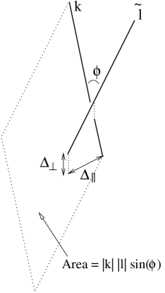
Figure 5: Maximally contributing configurations of two Wilson lines.

For $\Delta_{\parallel}$ in the region described, the minimum distance between the two lines will be $|\Delta_{\perp}|$. We expect that the main contribution to the integral will be from the region in which most of the propagators have length of the same order of magnitude as this minimum length. In this case, most of the propagator endpoints remain within a distance of roughly ${|\Delta_{\perp}|\over\phi}$ from the crossing point. The average separation between endpoints on each line will therefore be roughly $\min\left({|\Delta_{\perp}|\over n\phi},{|\tilde{k}|\over n}\right)$.

If the average separation between the endpoints is much greater than the average propagator length, it is a good approximation to extend the region of integration for each $\tau$ between $-\infty$ and $\infty$. This approximation will therefore be valid if

$$n<\min({1\over\phi},{|\tilde{k}|\over|\Delta_{\perp}|})$$ (34)

We will call this the small $n$ approximation, since there is an upper bound on $n$ (though it may be large). This generalizes the $\eta<1$ regime in our evaluation of two point function for which the saddle point approximation was justified (21). For $n$ larger than this bound, we will require other methods to evaluate the integral.

We now turn to a detailed evaluation of the integral ${\cal I}_{n}$ in both the small and large $n$ approximations. It will turn out that for weak coupling calculations, only the small $n$ regime is relevant, while for strong coupling, we require the large $n$ behavior.

5.3 Small $n$ Approximation

We begin by evaluating the integral ${\cal I}_{n}$ in the small $n$ regime. As discussed, for $n$ satisfying the bound (34) it is a good approximation to extend the integration region for the $\tau$’s to the whole real line for a typical set of $\sigma$’s (equivalent to a saddle point approximation). This also provides an upper bound on the integral for all values of $n$ and the other parameters.

After performing this saddle point evaluation, the remaining integral takes the form

$${\cal I}_{n}=\int_{0}^{1}d\sigma_{n}\cdots\int_{0}^{\sigma_{2}}d\sigma_{1}f(\sigma_{1})\cdots f(\sigma_{n}) = {1\over n!}(\int_{0}^{1}d\sigma f(\sigma))^{n}$$ (35)

$$\equiv {1\over n!}H^{n}$$

where

$$f(\sigma) = \int_{-\infty}^{\infty}d\tau{\lambda\tilde{k}\cdot\tilde{l}\over|\Delta+\tilde{k}\sigma-\tilde{l}\tau|^{2}}$$ (36)

$$= {\lambda\tilde{k}\cdot\tilde{l}\over\sqrt{\tilde{l}^{2}(\Delta+\tilde{k}\sigma)^{2}-(\tilde{l}\cdot(\Delta+\tilde{k}\sigma))^{2}}}$$

We can perform the the integral over $\sigma$ exactly, though the result is somewhat messy. In order to get an idea of the dependence on $\phi$ and $\tilde{k}$, it is illuminating to consider the case in which the lines have equal length.

The maximum contribution comes from the value of $\Delta_{\parallel}$ for which the lines cross symmetrically in the projection to the noncommutative directions. This occurs for $\Delta\cdot\tilde{k}=-{\tilde{k}^{2}\sin^{2}\phi/2}$, and in this case, the result is

$$H=\lambda\cot\phi\,\log\left({\sqrt{({\tilde{k}\sin\phi\over 2\Delta})^{2}+1}+{\tilde{k}\sin\phi\over 2\Delta}\over\sqrt{({\tilde{k}\sin\phi\over 2\Delta})^{2}+1}-{\tilde{k}\sin\phi\over 2\Delta}}\right)$$ (37)

Here, once again for the sake of brevity we denote by $\Delta$ the distance in the commutative directions, previously denoted as $\Delta_{\perp}$. Though we have chosen a particular value for $\Delta_{\parallel}$, we note that ${\cal I}_{n}$ should be roughly constant over the region of $\Delta_{\parallel}$ shown in figure 5 since the dominant configurations in the integral will have all propagators clustered around the crossing point.

Recalling that ${\cal I}_{n}=H^{n}/n!$, we see that for angles $\phi\ll{\Delta\over\tilde{k}}$,

$${\cal I}_{n}={1\over n!}\left(\lambda\,{\tilde{k}\over\Delta}(1-{\tilde{k}^{2}\phi^{2}\over 24\Delta^{2}}+\cdots)\right)^{n}$$ (38)

while for $\phi\gg{\Delta\over\tilde{k}}$, we get

$${\cal I}_{n}={1\over n!}\left(\lambda\,{1\over\phi}\ln\left(\tilde{k}\phi\over\Delta\right)\right)^{n}$$ (39)

These formulae accurately describe the behavior of ${\cal I}_{n}$ in the small $n$ regime, (34).

5.4 Large $n$ Approximation

We now consider the case in which the small $n$ approximation is no longer valid. This occurs when the average separation between points on each line becomes less than the typical distance between the lines. In this limit, the propagator endpoints become dense on the two lines, and we expect that most of the contribution to the integral comes from a small region about some preferred configuration.

To get an idea of the $\tilde{k}$ and $\phi$ dependence of ${\cal I}_{n}$ in the large $n$ regime, we again take the simple configuration with $|\tilde{k}|=|\tilde{l}|$ and $\Delta_{\parallel}=0$ (this is the configuration shown in figure 4 if the separation $\Delta$ in the diagram is understood to be perpendicular to the lines). Since the integrals are difficult to evaluate directly in the large $n$ regime, we will determine the behavior of ${\cal I}_{n}$ by establishing upper and lower bounds.

5.4.1 Large $n$, Upper Bound

First, we will determine an upper bound on ${\cal I}_{n}$ for this configuration using the relation

$$\int|f_{1}\cdot f_{2}\cdots f_{n}|\leq(\int|f_{1}|^{n})^{1\over n}\cdots(\int|f_{n}|^{n})^{1\over n}$$ (40)

where $f_{i}$ are arbitrary functions on some integration region (this is a generalization of the Cauchy-Schwarz inequality). This implies that

$${\cal I}_{n}\leq(\prod_{m=1}^{n}\hat{{\cal I}}_{m})^{1\over n}$$ (41)

where $\hat{{\cal I}}_{m}$ is obtained from ${\cal I}_{n}$ by replacing the product of propagators in the integrand by $n$ copies of the $m$th propagator. The integrals $\hat{{\cal I}}_{m}$ are much easier to evaluate, as we will see.

The integrand of $\hat{{\cal I}}_{m}$ depends only on $\sigma_{m}$ and $\tau_{m}$, and it is straightforward to perform the integrals over all other $\sigma$s and $\tau$s. We find

$$\hat{\cal I}_{m}=(\lambda\tilde{k}\cdot\tilde{l})^{n}\int_{0}^{1}d\sigma_{m}\int_{0}^{1}d\tau_{m}\;{f(\sigma_{m})\;f(\tau_{m})\over|\Delta+\tilde{k}\sigma_{m}-\tilde{l}\tau_{m}|^{2n}}$$ (42)

where

$$f(t)={t^{m-1}(1-t)^{n-m}\over(m-1)!(n-m)!}$$ (43)

We note that $f(t)$ is sharply peaked at $t={m-1\over n-1}$ while the denominator of $\hat{\cal I}_{m}$ is sharply peaked near $\sigma=\tau=0$. The integral will receive most of its contribution from these two regions. For small enough $\Delta$, it is the latter region near the origin that dominates, since, as we will see, ${\cal I}_{n}$ diverges as $\Delta\to 0$. It is convenient to rewrite the integral in terms of $\sigma_{+}=\sigma+\tau$ and $\sigma_{-}=\sigma-\tau$. This gives

$$\hat{\cal I}_{m} = {\lambda^{n}\tilde{k}^{2n}\cos^{n}\phi\over[(m-1)!(n-m)!]^{2}}$$

$$\hskip 21.68121pt{1\over 2}\int_{0}^{2}d\sigma_{+}\int d\sigma_{-}{({1\over 4}(\sigma_{+}^{2}-\sigma_{-}^{2}))^{m-1}((1-{1\over 2}\sigma_{+})^{2}-{1\over 4}\sigma_{-}^{2})^{n-m}\over(\Delta^{2}+\tilde{k}^{2}\cos^{2}({\phi\over 2})\sigma_{-}^{2}+\tilde{k}^{2}\sin^{2}({\phi\over 2})\sigma_{+}^{2})^{n}}$$

The $\sigma_{-}$ integral is sharply peaked at $\sigma_{-}=0$ and may be evaluated using the saddle point approximation. Near $\sigma_{+}=0$, the result (for $m>1$) is

$$\hat{\cal I}_{m}={\lambda^{n}\tilde{k}^{2n}\cos^{n}\phi\over 2^{2m-1}[(m-1)!(n-m)!]^{2}}\sqrt{\pi\over m-1}\int_{0}d\sigma_{+}{\sigma_{+}^{2m-1}(1-{1\over 2}\sigma_{+})^{2n-2m}\over(\Delta^{2}+\tilde{k}^{2}\sin^{2}({\phi\over 2})\sigma_{+}^{2})^{n}}$$ (46)

The dominant term for small $\Delta$ ($\Delta<\tilde{k}\phi$) may now be computed exactly, and we find (for $1<m<n$)

$$\hat{\cal I}_{m}={\lambda^{n}\over[(n-1)!]^{2}}{n-1\choose m-1}{1\over 4^{m}(n-m)\sqrt{m-1}}{\cos^{n}\phi\over\sin^{2m}{\phi\over 2}}\left({\tilde{k}^{2}\over\Delta^{2}}\right)^{n-m}$$ (47)

Finally, using the relation (41) we find an upper bound for $\phi>\tilde{k}/\Delta$ (ignoring constants)

$${\cal I}_{n}\leq{\lambda^{n}\over(n!)^{2}}\left({\tilde{k}\cos\phi\over\Delta\sin{\phi\over 2}}\right)^{n}$$ (48)

Proceeding from equation (46) for $\phi<\tilde{k}/\Delta$ we find

$${\cal I}_{n}\leq{\lambda^{n}\over(n!)^{2}}\left({\tilde{k}\over\Delta}\right)^{2n}\left(1-{\tilde{k}^{2}\phi^{2}\over 3\Delta^{2}}+\dots\right)^{n}$$ (49)

5.4.2 Large $n$, Lower Bound

We now determine a lower bound on ${\cal I}_{n}$ in the large $n$ regime. To do this, we restrict the integration region by choosing an ordered set $0=a_{0}\leq a_{1}\leq\cdots\leq a_{n}-1\leq a_{n}=1$ such that

$$a_{i}<\sigma_{i},\tau_{i}<a_{i+1}$$ (50)

Then certainly,

$${\cal I}_{n}\geq\prod\int_{a_{i}}^{a_{i+1}}d\sigma_{i}\int_{a_{i}}^{a_{i+1}}d\tau_{i}{\lambda\tilde{k}\cdot\tilde{l}\over|\Delta+\tilde{k}\sigma-\tilde{l}\tau|^{2}}\\$$ (51)

This bound is valid for all choices of $a_{i}$, so in order to establish the best lower bound, we would like to maximize the last expression over all such choices. Despite a great reduction in the size of the integration region, this approach actually gives a reasonable estimate of ${\cal I}_{n}$ for large $n$ since the full integral is dominated by contributions from a very small region about some preferred configuration, and the maximization over choices of $a_{i}$ essentially selects this dominant region.

Since we take $n$ to be very large, the values $a_{i}$ are very closely spaced. We therefore can define a continuous functions $f(x)$, such that:

$$a_{i}=f(\frac{i}{n})$$ (52)

This satisfies the boundary conditions:

$$f(0)=0\qquad\qquad f(1)=1$$ (53)

Taking logarithms of both sides of (51) and replacing the sum by an integral we then obtain

$$\log\left({{\cal I}_{n}\over\lambda^{n}(\tilde{k}\cdot\tilde{l})^{n}}\right)\geq G_{n}(f)\;,$$ (54)

where

$$G_{n}(f) = n\,\int_{0}^{1}dx\{2\log(f^{\prime}(x){1\over n})-\log(|\Delta+\tilde{k}f(x)-\tilde{l}f(x)|^{2})\}$$ (55)

$$= -2n\log(n)+n\,\int_{0}^{1}dx\{2\log(f^{\prime}(x)-\log({\Delta_{\perp}}^{2}+f^{2}S^{2})\}\;$$ (56)

Here, we have defined $S=2|\tilde{k}|\sin(\frac{\phi}{2})$, and to avoid clutter, we omit the subscript in $\Delta_{\perp}$.

We now maximize $G$ by solving the Euler-Lagrange equation for $f$. This gives

$$2\log(f^{\prime})-\log(\Delta^{2}+f^{2}S^{2})=C\\$$ (57)

where $C$ is a constant.

Solving this and choosing integration constants to satisfy the boundary conditions (53), we find

$$f_{min}(x)={\Delta\over S}\sinh(x\cdot\sinh^{-1}({S\over\Delta}))$$ (58)

It is now simple to plug this value of $f_{min}$ into $G$ to obtain a lower bound

$${\cal I}_{n} \geq (\lambda\tilde{k}\cdot\tilde{l})^{n}e^{G(f_{min})}$$ (59)

$$= {\lambda^{n}\cos^{n}\phi\over n^{2n}}\left({1\over 2\sin{\phi\over 2}}\sinh^{-1}\left({2\tilde{k}\sin{\phi\over 2}\over\Delta}\right)\right)^{2n}$$

For $\tilde{k}\phi\ll\Delta$ , which includes the exactly antiparallel case, this gives

$${\cal I}_{n}\geq{\lambda^{n}\cos^{n}\phi\over n^{2n}}\left({\tilde{k}\over\Delta}\right)^{2n}\left(1-{1\over 6}\left({2\tilde{k}\sin{\phi\over 2}\over\Delta}\right)^{2}+\dots\right)^{2n}$$ (60)

while for $\tilde{k}\phi\gg\Delta$ (the non-parallel case for small enough $\Delta$) we get

$${\cal I}_{n}\geq{\lambda^{n}\cos^{n}\phi\over n^{2n}}\left({1\over 2\tilde{k}\sin{\phi\over 2}}\log\left({4\tilde{k}\sin{\phi\over 2}\over\Delta}\right)\right)^{2n}$$ (61)

Note also that

$$n^{2n}=e^{2(n\ln(n)-n)}e^{2n}\approx(n!)^{2}e^{2n}$$ (62)

so for example in the antiparallel case, we have upper and lower bounds

$${1\over(n!)^{2}}{1\over(e\Delta)^{2n}}\leq{\cal I}_{n}\leq{1\over(n!)^{2}}{1\over\Delta^{2n}}$$ (63)

This justifies the claim in section 2 that the upper bound provides a good estimate of $I_{n}$ in the large $n$ regime for the antiparallel case.

We have now determined the behavior of ${\cal I}_{n}$ for general values of $n$ and the other parameters. In the next section we summarize these results and discuss the physical consequences for the behavior of the correlation functions at various values of the parameters.

6 Summary of Results

We have considered correlation functions of the form

$$\langle W_{1}(k)W_{2}(-l)\cdots W_{n}(k_{n})\rangle$$ (64)

and noted that even at weak coupling, ladder diagrams connecting $W_{1}$ and $W_{2}$ must be included when the momenta $k$ and $-l$ are nearly antiparallel, as summarized in figure 3. For the ladder diagram contributions, the dependence on $k$ and $l$ is given by

$$\langle W_{1}(k)W_{2}(-l)\cdots W_{n}\rangle\sim\int d^{4}\Delta\exp(i\Delta\cdot(k-l)/2)f(\Delta,\cdots)\sum_{n}{\cal I}_{n}$$ (65)

where $f$ represents the commutative position space correlator and ${\cal I}_{n}$ is defined in (33).

Figure 6: Regimes of behavior for ${\cal I}_{n}$ in the $\Delta-n$ plane.

Our results for the behavior of ${\cal I}_{n}$ are summarized in figure 6. For momenta of magnitude $k$ with a given fixed angle $\phi$ between the, we find four regions of behavior as $n$ and $\Delta$ are varied:

small n:

In this regime, defined by

$$n<\min({1\over\phi},{\tilde{k}\over\Delta})\;,$$ (66)

the typical spacing between points on the Wilson lines is greater than the average separation between the lines (propagator length). We find that

$${\cal I}_{n}=\left\{\begin{array}[]{ll}{1\over n!}\left(\lambda\,{\tilde{k}\over\Delta}(1-{\tilde{k}^{2}\phi^{2}\over 24\Delta^{2}}+\cdots)\right)^{n}&\qquad\qquad{\tilde{k}\over\Delta}\ll{1\over\phi}\\ {1\over n!}\left(\lambda\,{1\over\phi}\log({\tilde{k}\phi\over\Delta})\right)^{n}&\qquad\qquad{\tilde{k}\over\Delta}\gg{1\over\phi}\end{array}\right.$$ (67)

These correspond to regions $A$ and $B$ respectively in figure 6.

large n:

In this regime, for which

$$n>\min({1\over\phi},{\tilde{k}\over\Delta})\;,$$ (68)

the points are densely packed on the two Wilson lines. For ${\tilde{k}\over\Delta}>{1\over\phi}$ (region $D$) we have determined upper and lower bounds given by

$${\lambda^{n}\cos^{n}\phi\over(n!)^{2}}\left({1\over 2\sin{\phi\over 2}}\log\left({4\tilde{k}\sin{\phi\over 2}\over\Delta}\right)\right)^{2n}\leq{\cal I}_{n}\leq{\lambda^{n}\over(n!)^{2}}\left({\tilde{k}\cos\phi\over\Delta\sin{\phi\over 2}}\right)^{n}$$ (69)

Finally, in region $C$ with ${\tilde{k}\over\Delta}<{1\over\phi}$ we find

$${\lambda^{n}\over n^{2n}}\left({\tilde{k}\over\Delta}\right)^{2n}\left(1-{1\over 6}\left({\tilde{k}\phi\over\Delta}\right)^{2}+\dots\right)^{2n}\leq{\cal I}_{n}\leq{\lambda^{n}\over(n!)^{2}}\left({\tilde{k}\over\Delta}\right)^{2n}\left(1-{\tilde{k}^{2}\phi^{2}\over 3\Delta^{2}}+\dots\right)^{n}$$

In evaluating the momentum space correlators, we must sum over $n$ and integrate over $\Delta$ as in equation (32). In this case, because of the additional $\Delta$ dependence of the function $f(\Delta)$ in (32), it is simplest to consider first the sum over $n$ with everything else fixed.

Note that as a function of $n$, the series of terms ${\cal I}_{n}$ is exponential (${\cal I}_{n}\sim{H^{n}\over n!}$) in the small $n$ regime and then falls of faster (${\cal I}_{n}\sim{G^{n}\over(n!)^{2}}$)in the large $n$ regime. Thus, it is obvious that the series converges for any values of the parameters. Furthermore, just as for the two point function, there will be some $M$ such that the terms start decreasing for $n>M$, and terms with $n\gg M$ will give negligible contribution.

At weak coupling ($\lambda\ll 1$), we find that $M$ lies well within the small $n$ regime as long as

$$\phi<{\Delta\over\tilde{k}}e^{1\over\lambda}\;.$$ (70)

In this case, the large $n$ terms have negligible contribution and we find

$$\begin{array}[]{ll}\sum{\cal I}_{n}=e^{\lambda\,{\tilde{k}\over\Delta}}\cdot e^{-{\tilde{k}^{2}\phi^{2}\over 24\Delta^{2}}}&\qquad\qquad\phi\ll{\Delta\over\tilde{k}}\\ \sum{\cal I}_{n}=\left({\tilde{k}\phi\over\Delta}\right)^{\lambda\over\phi}&\qquad\qquad{\Delta\over\tilde{k}}\ll\phi<\lambda\log{\tilde{k}\over\Delta}\end{array}$$ (72)

For larger angles, ladder diagrams are no longer important and the result will be given by the leading order in perturbation theory.

For strong coupling $\lambda\gg 1$, $M$ lies in the large $n$ regime. In this case, the series is dominated by terms in the large $n$ region, and we find (for small angles)

$$\begin{array}[]{ll}e^{\sqrt{\lambda}\tilde{k}\over e\Delta}e^{-{1\over 6}\left({\tilde{k}\phi\over\Delta}\right)^{2}}\leq\sum{\cal I}_{n}\leq e^{\sqrt{\lambda}\tilde{k}\over\Delta}e^{-{1\over 3}\left({\tilde{k}\phi\over\Delta}\right)^{2}}&\qquad\qquad\phi\ll{\Delta\over\tilde{k}}\\ \left({2\tilde{k}\phi\over\Delta}\right)^{\sqrt{\lambda}\over\phi}\leq\sum{\cal I}_{n}\leq\exp\left(\sqrt{2\lambda\tilde{k}\over\phi\Delta}\right)&\qquad\qquad\phi\gg{\Delta\over\tilde{k}}\end{array}$$ (74)

The detailed form of the correlation functions would now be obtained by inserting these expressions for ${\cal I}_{n}$ into the expression (32) and integrating over $\Delta$. However, the universal behavior at large momenta, including the angular dependence, is already quite clear from the various expressions for ${\cal I}_{n}$.

We see that both for the weak coupling and the strong coupling expressions, $\sum{\cal I}_{n}$ is very sharply peaked near $\phi=0$, and decays very rapidly for $\phi>{\Delta\over\tilde{k}}$. Roughly, the typical value of $\Delta$ in the Fourier transform will be ${1\over k}$ so we see that there is a critical angle $\phi={1\over k\tilde{k}}$ below which the correlation functions are strongly enhanced. For $\phi=0$ we get precisely the exponential dependence on momenta that was observed in the two point functions.

In [16], it was pointed out that in the absence of a natural normalization of individual operators the most meaningful objects to consider are normalization independent ratios of correlation functions,

$${\langle W_{1}(k_{1})W_{2}(k_{2})\cdots W_{n}(k_{n})\rangle\over\langle W_{1}(k_{1})W_{1}(-k_{1})\rangle^{1\over 2}\cdots\langle W_{n}(k_{n})W_{n}(-k_{n})\rangle^{1\over 2}}$$ (75)

They argued that the exponential behavior of the two-point functions would generally lead to exponential suppression of the correlation functions at high momenta. Given our results, we see that this will be true for generic angles, however, if the momenta of two operators become pairwise antiparallel ($\phi\ll{1\over k\tilde{k}}$), the numerator will also exhibit exponential behavior that should precisely cancel the exponential behavior in the denominator. In this case, the momentum dependence is no longer universally determined by the Wilson line contribution. Rather it is determined by the correlation functions of the local operators attached to the Wilson line. Therefore we expect that it reverts to more typical field theoretic behavior. In particular, in the planar limit the behavior is determined by the UV fixed point of the commutative version of the theory. It would be very interesting to understand the meaning of the angular dependence we have observed from the point of view of the gravity dual, but we leave this as a question for future work.

References

- [1] A. Connes, M. R. Douglas and A. Schwarz, “Noncommutative geometry and matrix theory: Compactification on tori,” JHEP 9802, 003 (1998) [hep-th/9711162].
- [2] M. R. Douglas and C. Hull, “D-branes and the noncommutative torus,” JHEP 9802, 008 (1998) [hep-th/9711165].
- [3] V. Schomerus, “D-branes and deformation quantization,” JHEP 9906, 030 (1999) [hep-th/9903205].
- [4] N. Seiberg and E. Witten, “String theory and noncommutative geometry,” JHEP 9909, 032 (1999) [hep-th/9908142].
- [5] S. Minwalla, M. Van Raamsdonk and N. Seiberg, “Noncommutative perturbative dynamics,” hep-th/9912072; M. Van Raamsdonk and N. Seiberg, “Comments on noncommutative perturbative dynamics,” JHEP 0003, 035 (2000) [hep-th/0002186].
- [6] A. Matusis, L. Susskind and N. Toumbas, “The IR/UV connection in the non-commutative gauge theories,” hep-th/0002075.
- [7] J. Maldacena, “The large N limit of superconformal field theories and supergravity,” Adv. Theor. Math. Phys. 2, 231 (1998) [hep-th/9711200].
- [8] A. Hashimoto and N. Itzhaki, “Non-commutative Yang-Mills and the AdS/CFT correspondence,” Phys. Lett. B465, 142 (1999) [hep-th/9907166].
- [9] J. M. Maldacena and J. G. Russo, “Large N limit of non-commutative gauge theories,” JHEP 9909, 025 (1999) [hep-th/9908134].
- [10] S. Das,S. Rama and S. Trivedi, “Supergravity with Self-dual fields and Instantons in Noncommutative Gauge Theory,” JHEP 0003, 004 (2000) [hep-th/9911137].
- [11] M. Berkooz, “Non-local field theories and the non-commutative torus,” Phys. Lett. B430, 237 (1998) [hep-th/9802069].
- [12] N. Ishibashi, S. Iso, H. Kawai and Y. Kitazawa, “Wilson loops in noncommutative Yang-Mills,” Nucl. Phys. B573, 573 (2000) [hep-th/9910004].
- [13] J. Ambjorn, Y. M. Makeenko, J. Nishimura and R. J. Szabo, JHEP 9911, 029 (1999) [hep-th/9911041].
- [14] J. Ambjorn, Y. M. Makeenko, J. Nishimura and R. J. Szabo, Phys. Lett. B480, 399 (2000) [hep-th/0002158].
- [15] J. Ambjorn, Y. M. Makeenko, J. Nishimura and R. J. Szabo, JHEP 0005, 023 (2000) [hep-th/0004147].
- [16] D. J. Gross, A. Hashimoto and N. Itzhaki, “Observables of non-commutative gauge theories,” hep-th/0008075.
- [17] S. R. Das and S. Rey, “Open Wilson lines in noncommutative gauge theory and tomography of holographic dual supergravity,” Nucl. Phys. B590, 453 (2000) [hep-th/0008042].
- [18] A. Dhar and S. R. Wadia, “A note on gauge invariant operators in noncommutative gauge theories and the matrix model,” hep-th/0008144.
- [19] D. Bigatti and L. Susskind, “Magnetic fields, branes and noncommutative geometry,” Phys. Rev. D62, 066004 (2000) [hep-th/9908056].
- [20] J. K. Erickson, G. W. Semenoff and K. Zarembo, “Wilson loops in N = 4 supersymmetric Yang-Mills theory,” Nucl. Phys. B582, 155 (2000) [hep-th/0003055].
- [21] N. Drukker and D. J. Gross, “An exact prediction of N = 4 SUSYM theory for string theory,” hep-th/0010274.
- [22] H. Liu, “*-Trek II: *n operations, open Wilson lines and the Seiberg-Witten map,” hep-th/0011125.
- [23] S. R. Das and S. P. Trivedi, “Supergravity couplings to noncommutative branes, open Wilson lines and generalized star products,” hep-th/0011131.
- [24] O. Aharony, M. Berkooz, D. Kutasov and N. Seiberg, “Linear dilatons, NS5-branes and holography,” JHEP 9810, 004 (1998) [hep-th/9808149].