Chapter 1 Introduction

There is no doubt that, at the fundamental level, theoretical physics is in the need of reconciling General Relativity and quantum theory. This becomes obvious already from Einstein’s equations

$$G_{\mu\nu}=\frac{8\pi G}{c^{2}}T_{\mu\nu}\,.$$ (1.1)

Here $G_{\mu\nu}$ is the Einstein tensor, determined solely in terms of the metric $g$, which governs the ‘gravitational force’, and $T_{\mu\nu}$ is the energy momentum tensor of matter fields. We know that matter fields are governed by a quantum field theory, the standard model of strong and electroweak interactions. Equations (1.1), however, contain purely classical, commuting quantities. On the other hand, Einstein’s equations show that, in the presence of matter, $T_{\mu\nu}\neq 0$, the metric $g$ can not be strictly Minkowskian (since then $G_{\mu\nu}\neq 0$); it can be so at best to some approximation. A Minkowski background metric is used, however, in standard quantum field theory of elementary particle physics.

Certainly, no current experiments in our laboratories come only close to explicitly display the above contradiction experimentally. Still, from the point of view of a unified and mathematically consistent theory of all interactions, a new theory is needed.

There is a variety of (at least apparently) different contemporary approaches to improve on this situation: It ranges from noncommutative geometry [1], over twistors [2], over the attempt to quantize Einstein gravity nonperturbatively in a canonical fashion [3], to the advent of string theory [4], to name just the most prominent directions. The at the moment probably most promising of these attempts is the string approach. But also string theory is surely not formulated in a fully satisfactory and self-consistent way yet.

Black holes appear to provide an important link between gravity and quantum theory. First, near a black hole (and in particular near the singularity) the gravitational field cannot be ignored or approximated sufficiently well by a flat, Minkowskian metric. Second, the discovery of Hawking radiation [5] demonstrated that quantum effects cannot be ignored for black holes; rather they lead to a (slow, but still nonvanishing) evaporation of the classically indissoluble objects. Moreover, theoretical considerations allow to establish a striking analogy between the laws of thermodynamics and the laws governing black holes in classical general relativity [6]. Further Gedankenexperiments [7] show that the second law of thermodynamics should be altered to include an additive contribution to the entropy, assigned to the black hole. Already on dimensional grounds, the Planck length $l_{P}=\sqrt{\hbar G/c^{3}}$ enters the generalized second law of thermodynamics postulated in this way. It is felt by many contemporary theoreticians that black holes will be the gate to some fundamentally new picture of our world, bringing together seemingly separate subjects such as gravity, quantum theory, and thermodynamics.

As a side-remark let me mention that by now certainly black holes are no more purely theoretical objects. There is already overwhelming experimental evidence for the existence of black holes in the center of many galaxies, including ours (cf., e.g., [8]). Also black holes have been found as partners in binary systems [9].

It is one of the famous results of General Relativity, called the no–hair theorem [10], that within Einstein–Maxwell theory all asymptotically flat, stationary black holes are determined uniquely by specification of their mass $m$, their charge $q$, and their angular momentum $J$. This scenario extends to some other matter couplings such as to the case of additional scalar fields (with convex potential). Still, the ‘no–hair conjecture’ does not hold in full generality: counter examples have been found recently (cf references in [10]) such as, e.g., in the Einstein–Yang–Mills theory with gauge group $SU(2)$ (note that these solutions are unstable, however). Thus, (in those cases where the no–hair theorem or conjecture holds) the space of (stationary) black hole solutions (modulo gauge transformations) is finite dimensional only.

The formulation of gravity in two spacetime dimensions allows to isolate precisely these most interesting objects of General Relativity: Upon definition of appropriate two–dimensional gravitational actions, cf. chapters 2 and 3 below, the space of their classical solutions does not only contain (two–dimensional) black holes, it consists only of such spacetimes, except possibly for naked singularity solutions and a vacuum ground state. Many of the considerations performed for their four–dimensional analogs, moreover, like the prediction of Hawking radiation as well as the analogy to thermodynamics, may be transferred also into the two–dimensional setting. Finally, also here the original theory is invariant with respect to diffeomorphisms (the group of coordinate transformations), such that a transition to the quantum theory is plagued by similar conceptual difficulties as in four spacetime dimensions (like the ‘problem of time’ [11] to name just one of them).

During about the last decade, two–dimensional gravity models thus turned out as an interesting and promising theoretical laboratory to test ideas on how to approach quantization of gravity. Hundreds of works appeared within this field. Still, on many of the main, fundamental questions, even in this simplified context, no final conclusion or consensus has been reached by now.

The present work focuses on the foundation of such investigations of the two–dimensional world of gravity. It is felt that a good and sound understanding of the classical aspects, which, as we will show, are also far from trivial, provides a necessary basis for tackling issues of quantum gravity and quantum black holes. Emphasis has been put on exactly solvable models in this context.

Only at the very end of this report we dare a glance into the 2d quantum world. In particular, we will apply one particular quantization scheme to pure gravity Yang–Mills systems, comparing the final result with the preceding classical considerations. We did not attempt to also include a decent account of all developments on the quantization of 2d gravity models. The thermodynamics and Hawking evaporation of such models, which fill large portions of the 2d gravity activity, are not discussed in this report (except for some remarks).

The organization of the present survey is as follows: In chapter 2 we provide some of the basic geometrical ingredients and then construct and motivate a wide class of two–dimensional models of (pure) gravity. In the subsequent chapter this class of models is even enlarged further, while additional motivation is found, e.g., in regarding invariant sectors of four–dimensional gravity as effectively two–dimensional theories. The addition of various types of matter fields is discussed in this chapter, too. In chapter 4, a $\sigma$–model is presented, which allows for a unifying and elegant treatment of the whole class of gravity models discussed before (including Yang–Mills fields, but preferably in the absence of further matter). This formulation proves a powerful tool for the analysis on the classical as well as on the quantum level in subsequent chapters.

Chapters 5 and 6 contain a careful discussion of various aspects of the classical solutions. In particular, for the gravity Yang–Mills models a complete classification of all possible global solutions is presented. The resulting spacetimes are in part highly nontrivial, including multi black holes, twists of the causal structure, and spacetimes of almost arbitrarily complicated (two–dimensional) topology.

The final chapter turns to the quantization of these models. Here the main part focuses on a canonical, Hamiltonian approach of quantization. The physical quantum states are found and compared to the space of classical solutions. Open issues, like the construction of an inner product between physical states, are addressed. Topics as approaches to Hawking radiation of 2d black holes are touched on only briefly.

The present work would not have been possible without, in particular, two people, who collaborated with me over several years within the subject: Peter Schaller and Thomas Klösch. The joint discovery of Poisson $\sigma$–models with P. Schaller [12], on the one hand, and the exhaustive investigation of global classical features of spacetimes performed in [13], on the other hand, need a word of mention here. I am grateful to these two people for permitting me to adapt some of this material for the present survey.

Chapter 2 2d geometry and gravitational actions

In this chapter we introduce and motivate 2d actions of $f(R)$–type gravity theories and extensions with nontrivial torsion. The actions discussed here will be purely geometrical, i.e. they are functionals of geometrical quantities only. Eventual dilaton–like fields enter as auxiliary fields only and, in contrast to the models discussed in the subsequent chapter, they are not necessary for the formulation of the action. The relation of the actions in terms of purely geometrical quantities and their reformulation in terms of auxiliary fields is made clear.

The present chapter provides the notation and conventions used within this work. It also contains some relations peculiar to two dimensions (some further 2d peculiarities may be found in section 6.1.2 below).

In the Introduction we already provided some motivation for studying two–dimensional gravity theories. Some additional, in part complementary reasons may be found in sections 2.5 and 2.6, where we also address the question of why the consideration of a whole class of gravity models is of interest, too.

2.1 From four to lower dimensions

One of the appealing features of Einstein’s theory of gravitation is that the ‘mediator of the gravitational force’ (thinking in terms of the old, Newtonian language) is an intrinsically geometrical object characterizing spacetime itself, namely its own metric $g$. Ultimately, this is a consequence of the principle of equivalence, the conceptual basis of Einstein’s theory of general relativity. The Einstein–Hilbert action, governing the dynamics of the metric $g$, is the simplest conceivable geometrical object yielding a coordinate independent local action:

$$\frac{1}{16\pi G}\int d^{4}x\sqrt{-\mbox{det}\,g}\,R\,,$$ (2.1)

where $R$ is the (intrinsic) curvature scalar of the (metrical and torsion–free) connection, determined uniquely by $g$.

Generically, when studying toy models of a physical theory by reducing the dimension $D$ of spacetime, there are two possible routes: The first one is a Kaluza–Klein procedure, where, in its simplest form, one assumes the basic fields of the theory, which here is the metric, to be ‘independent’ of $n$ coordinate directions; then the action in $D$ dimensions induces an action in $D-n$ dimensions. The other standard (and simpler) route is to replace the $D$–dimensional action by its lower–dimensional analog.

While the latter approach truly yields a toy model, which will have similarities but also pronounced differences due to the generic simplification encountered when reducing the dimension of spacetime, the former approach captures a sector of the physical $D$– respectively four–dimensional theory. Models and actions resulting from a Kaluza–Klein approach are thus of particular interest. Such models will be discussed, among others, in the following chapter (cf in particular the beginning of the next section as well as section 3.4). Here we first turn to the second approach.

While almost any 4d action has a meaningful 2d analog, the action (2.1) does not (at least when one requires the functional to yield some nontrivial field equations). Variation of the $D$–dimensional analog of (2.1), $\int d^{D}x\sqrt{-\mbox{det}\,g}\,R$, with respect to the metric, yields the Einstein tensor

$$G_{\mu\nu}\equiv R_{\mu\nu}-{1\over 2}g_{\mu\nu}R\,.$$ (2.2)

In the absence of additional matter fields the Einstein equations are thus tantamount to requiring this tensor to vanish.

In two spacetime dimensions ($D=2$), however, the Einstein tensor (2.2) vanishes identically. This may be seen, e.g., as follows: The general symmetries $R_{\alpha\beta\gamma\delta}=R_{[\alpha\beta][\gamma\delta]}$ of the curvature tensor, the brackets indicating antisymmetrization, allow one to conclude

$$R_{\alpha\beta\gamma\delta}=-\frac{R}{2}\varepsilon_{\alpha\beta}\varepsilon_{\gamma\delta}\,,$$ (2.3)

in two dimensions. Here $\varepsilon_{\alpha\beta}$ are the components of the $\varepsilon$–tensor, related to the (numerical) $\varepsilon$–symbol $\varepsilon(\alpha\beta)$ by means of $\varepsilon_{\alpha\beta}=\sqrt{-\mbox{det}\,g}\,\varepsilon(\alpha\beta)$, where we will stick to the convention $\varepsilon(01)=+1$ throughout this work. Using $\varepsilon_{\alpha\beta}\varepsilon_{\gamma\delta}=g_{\alpha\delta}g_{\beta\gamma}-g_{\alpha\gamma}g_{\beta\delta}$, we then indeed obtain $R_{\alpha\beta}\equiv R^{\gamma}{}_{\alpha\gamma\beta}={1\over 2}Rg_{\alpha\beta}\Leftrightarrow G_{\alpha\beta}=0$ as a 2d identity, as we wanted to establish.

There is a simple alternative to see that the Einstein–Hilbert term does not yield any field equations in two spacetime dimensions: $\sqrt{-g}\,R$ is a total divergence in $D=2$. (Here, as well as in what follows, we use the abbreviation $\sqrt{-\mbox{det}\,g}=:\sqrt{-g}$.) This fact will become obvious in Einstein–Cartan variables, to be introduced further below.

Let us remark, however, that

$$\int_{M}d^{2}x\sqrt{-g}R$$ (2.4)

is sometimes used as a 2d action within, e.g., the Euclidean path integral, yielding a topological invariant of the manifold $M$, namely its Euler characteristic.

The lowest dimension where an action of the form (2.1) remains to make sense (also classically) is $D=3$. But even in three spacetime dimensions the Einstein–Hilbert term does not yield propagating gravitational modes. While in four spacetime dimensions the vacuum Einstein equations $R_{\mu\nu}=0$ allow for nontrivial gravitational excitations (like gravitational waves), in $D=3$ they imply that the spacetime is flat: $R_{\mu\nu\rho\sigma}=0$.

Before returning to the question of a geometrical action in two dimensions, we briefly dwell on the consequences of equation (2.3) for the geometry of any 2d spacetime. As is obvious from this relation, in $D=2$ the spacetime has to be flat already when the Ricci scalar $R$ vanishes. Moreover, all (algebraic) curvature invariants are determined completely by means of $R$.

This does not mean, however, that the geometry (i.e. the geometrical content of the spacetime modulo coordinate transformations) is completely fixed by means of the function $R$ already. We provide an explicit example for this: With an appropriate choice of coordinates $x^{0},x^{1}$ any 2d metric may be brought into the local form (cf section 5.1.1.1)

$$ds^{2}=2dx^{0}dx^{1}+k(x^{0},x^{1})(dx^{1})^{2}\,.$$ (2.5)

In terms of this metric the curvature scalar is $R={\partial_{0}}^{2}k$. Thus, for the particular choice $k=h_{0}(x^{0})+h_{1}(x^{1})$, the function $h_{1}$ drops out of the curvature (this applies also to the full tensor (2.3), since det$g=-1$ for a metric of the form (2.5)). However, while a metric with $h_{1}\equiv 0$ evidently has the Killing vector field (generator of an isometry) $\partial_{1}$, it may be shown by explicit calculation (but cf also below) that a metric with $h_{1}^{\prime}\neq 0$ has no Killing field, provided only that $h_{0}^{\prime\prime\prime}\neq 0$. (Here and in what follows a prime denotes differentiation with respect to the argument of the respective function.) As the existence of a Killing field is a geometrical feature of a spacetime, independent of the choice of coordinates representing a metric, the above family of spacetimes contain at least two geometrically distinct ones, despite the fact that all of these spacetimes have the same curvature scalar $R$.

2.2 Purely geometrical 2d actions

The simplest, purely geometrical candidate 2d gravitational action is of the form

$$\int d^{2}x\sqrt{-g}(\alpha R^{2}-2\Lambda)\,,$$ (2.6)

where $\alpha$ is a coupling constant and $-2\Lambda$ a cosmological constant. Note that while in four spacetime dimensions there are several independent quadratic curvature invariants, here all of them are proportional to just $R^{2}$. As in any dimension, an action of the form (2.6) yields field equations which are fourth order differential equations for the metric $g$ ($R$ containing two derivatives). Introducing an auxiliary field $\phi$, the number of derivatives may be reduced to two: One easily establishes the equivalence

$${1\over 2}\int d^{2}x\sqrt{-g}\,R^{2}\sim\int d^{2}x\sqrt{-g}\,[\phi R-{1\over 2}\phi^{2}]\,,$$ (2.7)

which holds on the classical as well as on the quantum level (Gaussian integral), since the field equations obtained from variation with respect to $\phi$ are purely algebraic in $\phi$.

More generally we may consider the purely geometrical action

$$L=\int_{M}d^{2}x\sqrt{-g}f(R)\,,$$ (2.8)

where $f$ is some arbitrary (sufficiently well-behaved) function of the curvature scalar. Such actions were proposed, and in part studied, by Schmidt [14] (cf also references therein; for a later work cf [15]).

Note that even in two dimensions this is by no means the most general conceivable diffeomorphism invariant local action. Only when supplementing $R$ with $R_{(;a;b\cdots;d)}$, where the round brackets indicate symmetrization, and allowing all possible contractions between any of these terms, the most general diffeomorphism invariant local action functional of a 2d metric $g$ can be constructed (cf [17]). Such gravitational actions will not be considered in the present work (and the author is also not familiar with literature where such possibilities were considered in any detail).

To illustrate the potential relevance of such terms from the geometrical point of view, however, we briefly return to the example of two nonisometrical spacetimes (2.5) defined by $k=h_{0}(x^{0})$ with $h_{0}^{\prime\prime\prime}\neq 0$ on the one hand and $k=h_{0}(x^{0})+h_{1}(x^{1})$, $h_{1}^{\prime}\neq 0$, on the other hand. As discussed above, here the invariant $R$ (and thus any purely algebraic invariant constructed from the Riemann tensor!) is not ‘fine’ enough to distinguish between the two spacetimes. However, using e.g. $(\nabla R)^{2}\equiv R_{;a}R^{;a}=-k[(\partial_{0})^{3}k]^{2}$ in addition to $R$ it is possible to separate the two spacetimes (coordinate–independently): A Killing vector field has to annihilate all (algebraic and nonalgebraic) curvature invariants simultaneously; $\partial_{1}$, however, annihilates $(\nabla R)^{2}$ only for the first of the two metrics considered.

It is also possible to reformulate the action (2.8) by means of an auxiliary field $\phi$ (at least locally, cf the remarks below). Consider an action of the form

$$L=\int_{M}d^{2}x\sqrt{-g}[\phi R-V(\phi)]\,,$$ (2.9)

where $V$ is again some sufficiently well-behaved function. The variation of (2.9) with respect to $\phi$ is algebraic in $\phi$ and thus also here $\phi$ may be eliminated by implementing the solution back into (2.9) (provided only $V^{\prime\prime}\neq 0$). This will yield an action of the form (2.8).

We remark on this occasion that in subsequent chapters we will refer to the auxiliary field $\phi$ as the dilaton field; note that in the present context it has been introduced as a purely auxiliary field within the framework of an entirely geometrical action (that is, a diffeomorphism invariant, local action functional of the metric only).

Assuming that $f$ and $V$ are (at least) $C^{2}$–functions and that their second derivatives are nonzero, any $f$ gives rise to a $V$ and vice versa. If $V$ is linear (as is the case in the so–called Jackiw–Teitelboim model [18] discussed in the subsequent chapter, cf equation (3.21)), clearly $\phi$ cannot be eliminated by means of its field equations and thus this choice of $V$ cannot give rise to an action of the type (2.8). This is reflected also in the relation $f^{\prime\prime}(V(\phi))=1/V^{\prime\prime}(\phi)$, which may be derived provided $V^{\prime\prime}\neq 0$ and which is seen to become singular precisely when $V^{\prime\prime}$ becomes zero (again primes denote differentiation with respect to the argument of the respective function). It is interesting to observe vice versa that the choice $f=R$, which was found above to yield no field equations, — or, more generally, the choice $f:=a+bR$, $a,b\in\mbox{{\sl I R}}$, which is singular for $a\neq 0$ —, also corresponds to a singular limit of $V$.

Note that in general the above bijection between $f$ and $V$ works only within some neighborhood of a given value of $\phi$. The bijection is global, iff one restricts to the class of convex functions ($R^{2}$–gravity providing the prototype of these). However, we might be interested, in a first step, in local solutions to the field equations of a model (2.8) with some nonconvex function $f$. If the zeros of $f^{\prime\prime}$ are isolated, the above method may still be applicable patchwise: For all classical solutions of the model (2.8) where $R$ does not constantly take the value of a critical point of $f^{\prime}$, smoothness of the solution guarantees that any point on spacetime where the value of $R$ is noncritical, has a neighborhood such that within this neighborhood the above mentioned bijection works. Thus there then exists a model (2.9) with identical local solutions. In this way much more general models (2.8) allow a discussion by means of the alternative description (2.9). The global information possibly lost within such a transition has then to be restored in a second step. E.g. there could be additional solutions to the field equations (2.8) with a constant critical value of $R$; the possibility for such additional de Sitter solutions has to be checked. Otherwise only the local solutions with values of $\phi$ below and above critical points (or lines) have to be patched together. With these cautionary remarks taken into account (which, in principle, may be adapted also to the quantum regime), it is then possible to trade in a Lagrangian (2.8) against a Lagrangian (2.9) — and vice versa!

2.3 Einstein–Cartan variables

For later purposes we also need a Einstein–Cartan or Palatini formulation of the above gravity theories. We first set the notation and conventions: Let us denote spacetime indices by Greek letters from the middle of the alphabet, taking values zero and one, $\mu,\nu,\ldots\,\in\{0,1\}$, and Lorentz indices (indices referring to an orthonormal frame) from the beginning of the Latin alphabet, with either $a,b,\ldots\in\{\underline{0},\underline{1}\}$ or, when using a null basis, $a,b,\ldots\in\{+,-\}$. (Indices from the beginning of the Greek alphabet, such as those used in equation (2.3), denote indices in a general basis — except in the context of 2d supergravity theories, where they will label spinor indices.)

Our metric $g$ has signature $(+,-)$. In terms of the vielbein or zweibein, we then have

$$g=e^{\underline{0}}e^{\underline{0}}-e^{\underline{1}}e^{\underline{1}}=2e^{+}e^{-}\,,$$ (2.10)

where here the product between the oneforms is understood as symmetrized tensor product. In (2.10) we made use of the convention $e^{\pm}:=(e^{\underline{0}}\pm e^{\underline{1}})/\sqrt{2}$ for introducing a light cone basis; in terms of this basis, raising and lowering indices is accomplished simply by replacing a lower $+$ ($-$) by an upper $-$ ($+$) and vice versa ($e^{+}=e_{-}$ etc.).

The sign ambiguity in the metric induced volume form, i.e. in the $\varepsilon$–tensor, will be fixed by choosing

$$\varepsilon=e^{\underline{0}}e^{\underline{1}}=e^{-}e^{+}\,.$$ (2.11)

Here, and in any other product of forms except for those yielding a metric, the product is understood as the antisymmetrized tensor product, i.e. as the wedge product: $e^{\underline{0}}e^{\underline{1}}\equiv e^{\underline{0}}\wedge e^{\underline{1}}$. By means of the standard decomposition of forms, $\varepsilon={1\over 2}\varepsilon_{ab}e^{a}e^{b}$, we conclude from (2.11) that $\varepsilon_{{\underline{0}}{\underline{1}}}=\varepsilon^{+-}=+1$.

Beside the zweibein $e^{a}\equiv e^{a}_{\mu}dx^{\mu}$, the Einstein–Cartan or spin connection $\omega^{a}{}_{b}\equiv\omega^{a}{}_{b\mu}dx^{\mu}$ is of importance (here $x^{\mu}$ are coordinates in some arbitrary chart of the two–dimensional spacetime $M$.) Metricity of the connection translates into antisymmetry with respect to its two Lorentz indices: $\omega_{ab}+\omega_{ba}=0$. This, in turn, implies that the spin connection is a $SO(D-1,1)$ Lie algebra valued oneform. In $D=2$ the Lorentz group is just one–dimensional and there is just one independent connection one–form $\omega$: $\omega_{ab}=\varepsilon_{ab}\,\omega$. Under a local Lorentz transformation, i.e. a change of the orthonormal basis, $e^{\pm}\to\exp(\pm\alpha)\,e^{\pm}$, where $\alpha$ is an arbitrary (smooth) function on $M$, $\omega\to\omega+d\alpha$, which is the standard gauge transformation of an abelian gauge field. The curvature of spacetime is characterized by the Lie algebra valued twoform $\Omega^{a}{}_{b}\equiv{1\over 2}R^{a}{}_{b\mu\nu}dx^{\mu}dx^{\nu}$, which is nothing but the curvature of the gauge field $\omega^{a}{}_{b}$. Since in $D=2$ this gauge field is abelian, the nonlinear terms in the connection do not contribute and one simply finds ${1\over 2}R^{a}{}_{b\mu\nu}dx^{\mu}dx^{\nu}=\varepsilon^{a}{}_{b}\,d\omega$. Combining this equation with equation (2.3), we infer

$$R\varepsilon=-2d\omega\,.$$ (2.12)

Using the Hodge duality operation $\ast$, defined (in the present context of Lorentzian signature) by means of the relations $\ast 1=\varepsilon$, $\ast\varepsilon=-1$, and $\ast e^{a}=\varepsilon^{a}{}_{b}e^{b}\Leftrightarrow\ast e^{\pm}=\pm e^{\pm}$, equation (2.12) is seen to be equivalent to $R=2\ast d\omega$.

The variables $e^{a}$ and $\omega$ form a description of gravity equivalent to the metrical one only when, in addition to the local Lorentz symmetry, they are also subject to a constraint. Beside curvature there is the geometrical notion of torsion, describing the (internal) ‘twist’ of the 2d surface. In Einstein–Cartan formulation, it is associated to the Lorentz vector valued torsion two–form

$$De^{a}\equiv de^{a}+\varepsilon^{a}{}_{b}\omega e^{b}\,.$$ (2.13)

The standard connection used in Einstein’s theory of gravity (as well as in all the actions discussed so far) is torsion–free: $De^{a}\equiv 0$. It is a well–known fact that the latter equation (together with metricity) determines the spin connection $\omega^{a}{}_{b}$ (and thus also the curvature) uniquely in terms of the vielbein. In two dimensions this relation may be brought into a particularly simple form:

$$\omega=(\ast de^{a})\,e_{a}\,.$$ (2.14)

(Since both the curvature as well as the metric $g$ are invariant with respect to local Lorentz transformations, the curvature is determined implicitly by means of $g$ alone also when using the Einstein–Cartan formalism.)

We are now also in the position to show that in two dimensions $\sqrt{-g}R$ is a total divergence. Indeed this is evident now in view of $\varepsilon=\sqrt{-g}\,d^{2}x$ (where $d^{2}x\equiv dx^{0}dx^{1}$) and equation (2.12). (Note, however, that here $\omega$ is understood as an implicit functional of the metric on behalf of equation (2.14); it does not seem to be possible to express $\sqrt{-g}R$ explicitly as a covariant total differential of $g$ itself.)

It is a noteworthy feature of the 4d Einstein-Hilbert action that, when expressed in terms of the vielbein and spin connection as independent variables, the torsion zero condition follows automatically upon variation of the action with respect to $e^{a}$ (provided the theory is not coupled to spinors, however!). This does not hold in the case of the 2d actions discussed in the present chapter. We thus may use the Einstein–Cartan formulation either viewing $\omega$ as an abbreviation for the right–hand side of equation (2.14) or implementing the torsion zero condition by means of extra Lagrange multiplier fields, making sure that introduction of the latter does not alter the theory, certainly. We will follow the second route mainly.

In this approach the $R^{2}$ action (2.6) becomes (for $\alpha:=-(1/4)$):

$$\int(\ast d\omega)d\omega-2\Lambda\varepsilon+X_{a}De^{a}\,,$$ (2.15)

with $\varepsilon$ given in equation (2.11), $De^{a}$ in equation (2.13), and $X^{a}$ being the Lagrange multipliers mentioned above. Variation with respect to $\omega$ yields an equation that may be solved uniquely for $X^{a}$ (this equation is algebraic in $X^{a}$, but, however, no more in $\omega$). So $X^{a}$ and $\omega$ may be eliminated simultaneously within the action (2.15), with $\omega$ in the first term being given by equation (2.14) — and thus indeed no additional degrees of freedom are introduced in this formulation as compared to (2.6). Note, however, that since the equations for $X^{a}$ are not purely algebraic in $\omega$, the equivalence is guaranteed only on the classical level; on the quantum level it needs to be checked separately (e.g. by means of a careful path integral argument) — or, one uses one of the two formulations (2.6) and (2.15) to define the quantum theory for both of them.

Similarly the general action (2.8) may be rewritten in terms of Einstein–Cartan variables. In its (at least locally) equivalent form (2.9), one finds for $L$ (now interpreted as functional of $e^{a},\omega,\phi$, and $X^{a}$):

$$L=-2\int\phi d\omega+{1\over 2}V(\phi)\varepsilon+X_{a}De^{a}\,.$$ (2.16)

Note that irrespective of the choice of $V$ (resp. $f$ in (2.8)), this action is of first order form, i.e. (in the variables now used) its field equations are all at most first order differential equations.

2.4 Extension to theories with nontrivial torsion

When working with Einstein–Cartan variables it may appear unnatural to impose the zero torsion condition by hand. In particular, using vielbein and spin connection as independent variables in the Einstein–Cartan formulation of pure $D=4$ Einstein gravity, torsion zero follows as one of the (vacuum) Einstein field equations. Thus, also in the 2d setting, we may be interested in a purely geometrical, diffeomorphism and Lorentz invariant local action constructed (merely) in terms of the independent one–forms $e^{a}$ and $\omega$. The most general action of this type which yields second order differential equations of motion is of the form

$$L^{KV}=\int[-{1\over 4}d\omega\wedge\ast d\omega-{1\over 2\alpha}De^{a}\wedge\ast De_{a}+{\Lambda\over\alpha^{2}}\varepsilon]\,,$$ (2.17)

and was proposed by Katanaev and Volovich [19].

More generally, we may consider the higher order theories

$$L^{grav}=\int_{M}d^{2}x\sqrt{-g}F(\tau^{2},R)\,,$$ (2.18)

where $\tau^{a}\equiv\ast De^{a}$, $\tau^{2}\equiv\tau^{a}\tau_{a}$, and $F$ is some (reasonable) function. This is the most general geometrical action constructed in terms of algebraic curvature and torsion invariants. We remind the reader that in (2.18) $\omega$ is considered as variable independent of the zweibein. In contrast, in equation (2.8), when formulated in Einstein–Cartan variables, $\omega$ is either to be understood as an abbreviation for the right–hand side of (2.14) or torsion zero has to be implemented by additional Lagrange multiplier fields $X^{a}$. Thus, a model defined by (2.18) with a function $F$ independent of $\tau^{2}$ does in general not coincide with a model of the form (2.8), but constitutes another, different model (where the torsion is not forced to vanish).

Suppose first that $F$ depends nontrivially on $\tau^{2}$. Then also here it is possible to reexpress the action in first order form by introducing auxiliary fields. Indeed, at least on a local and classical level, an action (2.18) (provided it is sufficiently generic, cf the discussion below) can be cast into the form:

$$L^{grav}=\int_{M}\,\,X_{a}De^{a}+\phi d\omega+W(X^{2},\phi)\,\varepsilon\,\,,$$ (2.19)

where $X^{2}\equiv X_{a}X^{a}\equiv 2X^{+}X^{-}$ and $W$ is some two–argument function of the indicated variables. Nontrivial dependence of $F$ on $\tau^{2}$ will be seen to require also $W$ to depend nontrivially on $X^{2}$. On the other hand, we now realize that a function $W$ depending merely on $\phi$ allows to cover the torsion–free case (2.16) resp. (2.8), too. Thus when working with (2.19) we simultaneously may cover the torsion–free case (with $f^{\prime\prime}\not\equiv 0$, but anything else is of no interest anyway, cf our previous discussion) as well as (2.18) with nontrivial explicit torsion dependence — and further conditions, which we will specify now.

To decide under what precise conditions models of the type (2.18) may be described equivalently by means of (2.19) and vice versa, the following relation between the functions $F$ and $W$ is helpful: They are nothing but Legendre transforms of one another! Indeed, using equation (2.12) and $De^{a}=-\tau^{a}\varepsilon$, and just naively equating the two actions (multiplying one of them by the irrelevant factor $-1$), we find $F(\tau^{2},R)=X_{a}\tau^{a}+{1\over 2}\phi R-W(X^{2},\phi)$. The process of eliminating $X^{a}$ and ${1\over 2}\phi$ from the right–hand side by means of the equations of motion, moreover, coincides precisely with the standard Legendre procedure. Thus (global/local) equivalence holds provided the Hessian of $F$ and $W$ (interpreted as function of three arguments $X^{a}$ and $\phi/2$!) is (globally/locally) nondegenerate.

The KV model (2.17) provides an example where the equivalence to (2.19) clearly holds on a classical and quantum level globally. It results upon the quadratic choice

$$W^{KV}=-\frac{\alpha}{2}X^{2}-\phi^{2}+\frac{\Lambda}{\alpha^{2}}\,.$$ (2.20)

However, also more general cases, where the Hessians vanish only on lower dimensional submanifolds, may be treated interchangably, if the treatment takes care of the global relation, too. Note that this holds also on the quantum level as the equations for $X^{a}$ and $\phi$ are purely algebraic. As the treatment in the subsequent chapters of this work will be careful to not miss any global effects, such ‘weakly degenerate’ cases are covered, too.

The above restriction on the Hessians of $W$ and $F$ as a condition for the bijection between respective models confirms also the difference noted between a model of the type (2.8) on the one hand and (2.18) with an $F$ that is torsion independent on the other hand. The latter yields a strictly degenerate Hessian of $F$. A model (2.8), in contrast, is described by a strictly degenerate $W$ (namely one that is independent of $X^{2}$).

Adapting the argumentation, the present perspective also illuminates the relation of (2.8) to (2.16) (i.e. to $W$ with trivial $X^{2}$ dependence): In this case $X^{a}$ ceases to be connected to $\tau^{a}$ via a Legendre transformation ($\tau^{a}\equiv 0$!), but it acts as Lagrange multiplier to enforce (2.14). After the (nonalgebraic) elimination of $\omega$ and $X^{a}$, we are back to the problem of relating (2.8) to (2.9). The one–argument functions $f$ and $V$ are now recognized as Legendre transforms of one another.

On the other extreme side not covered in the bijection of $F$ and $W$ is a function $F$ that is independent of $\tau^{2}$. Such models result from (2.19) with an $X^{2}$–independent $W$ when dropping the term $X_{a}De^{a}$ altogether:

$$L=\int_{M}\,\,\phi\,d\omega+W(\phi)\,\varepsilon\,\,,$$ (2.21)

In view of the simplicity of (2.21), it is plausible that such theories are quite different from the theories (2.19). As we will show in section 5.1.2.5 below, the field equations of (2.21) lead to constant curvature spaces with unrestricted metric $g$. Such theories appear somewhat ‘ill’ therefore.

Models of the general type (2.18) (restricted to the case of nontrivial torsion dependence of $F$) were considered recently in [20] and, in its equivalent form (2.19), in [21] (but cf also [22, 23, 24]). Particular cases thereof (in particular the KV–model, equation (2.17)) have been considered also before [25, 26, 27, 28, 29, 30].

2.5 Why so many different Lagrangians

We thus arrived at a wealth of acceptable two–dimensional purely geometrical actions, which, within the 2d setting, may be taken to play the role of the Einstein–Hilbert term (2.1) of 4d gravity. The question may arise why we do not restrict our attention to just one of the possible choices for a 2d gravity action. The reason for considering this large amount of different actions is at least three–fold:

First, as discussed above, in two spacetime dimensions the naive analog (2.4) of (2.1) is meaningless (but cf also the remarks following equation (2.4)). We thus used the ‘equivalence principle’ (in the sense that we restricted attention to a diffeomorphism invariant, geometrical, and local functional) as the main guiding principle for the construction of the action governing the dynamics of the gravitational variables. This opened a wide territory for possible Lagrangians. Restricting to the use of merely algebraic invariants, leads to the class of theories (2.8) or, if allowing for nonzero torsion, to (2.18). (In $D=2$ the class of ‘geometric–algebraic’ (local) actions is thus parameterized by just one function of one respectively two arguments.)

In four spacetime dimensions certainly there are even much more possibilities for the construction of covariant actions. However, there we also have the experiment and this singles out the simplest among the possible actions (cf, however, possible quantum corrections mentioned below).

Second, in $D=4$ gravity relatively little is known about higher order actions. The discussion of the theory resulting from the Einstein–Hilbert term alone is difficult enough already: compared to the size of the total space of all possible classical solutions (even if restricted to physically reasonable ones), only very few exact solutions are known and under control. Moreover, the quantization of the Einstein–Hilbert term alone, although subject of intensive endeavours (cf, e.g., the loop approach [3]), is still beyond our abilities. In $D=2$, on the other hand, it is technically possible to obtain several exact results (and we will present a lot of them in the sequel) about all of the actions discussed in this (and the beginning of the following) chapter.

Third, there are several concepts in gravity which are not very sensitive to the particular choice of an action. One such an example is the existence of black hole (or otherwise singular) solutions; only very particular Lagrangians will exclude such solutions. On the other hand, there are some results proven specifically for the 4d Einstein theory (2.1). Quantum contributions are expected to lead to corrections to this Lagrangian and it is not clear if those results still apply. Thus there is some interest in the generality of some statements, applying to a whole class of Lagrangians.

Here we have in mind e.g. the area theorem [31] proven for 4d Einstein gravity. It states that, under some (reasonable) conditions, the total area of the horizon of a black hole cannot decrease. This statement covers complicated dynamical processes such as collisions of black holes, which are otherwise hardly tractable even by approximations on the computer. The area theorem is just one of the cornerstones of the notable analogy [6] between general relativity and thermodynamics mentioned in the Introduction, the horizon area in the former theory playing the role of entropy in the latter one. It is not at all clear, if, and in what way, such an analogy may be maintained when the Einstein–Hilbert term (2.1) receives small, higher order corrections as predicted e.g. by string theory (cf also section 3.1.2 below). It turns out that, phrased appropriately general, most of the analogy between gravity and thermodynamics may be found even in the context of the two–dimensional theories considered above and in the subsequent chapter (cf, e.g., [32]). Certainly, it is no more the area of a black hole horizon which can play the role of entropy; after all, in two spacetime dimensions the horizon consists of just a point. However, there is a precisely formulated proposal of Wald [33, 17] for what the entropy of a black hole should be proportional to, which is devised for an arbitrary diffeomorphism invariant action in any spacetime dimension. In the specific case of the Einstein–Hilbert term this quantity reduces to the area of the horizon, but already higher order corrections destroy this geometrical interpretation. The formalism of Wald also yields a nonvanishing entropy for 2d black holes (coinciding with the quantities found (or postulated) in [32]). It is then e.g. an interesting question to see, in which subclass of 2d models this quantity also obeys a second law (generalizing the above area theorem).

Last but not least, although different members of the class of models (2.8) and (2.18) have many features in common, there are also some qualitatively new properties arising in some of them which are absent in one or the other particular case. Such properties turn up in particular when dealing with global aspects of the theories under discussion. To sharpen ones techniques in dealing with gravity theories in general, we do not want to limit the class of 2d models too much. After all, the problems arising e.g. in the quantization of 4d gravity may be expected to be still much more complicated than the most involved 2d cases.

In the subsequent chapter, we will thus even enlarge the number of models to consider. The models of the present chapter will then be referred to as ‘geometrical’ ones, as all of them may be formulated entirely in terms of geometrical variables only.

2.6 Why consider low–dimensional, topological models

Although not obvious at first sight, none of the gravitational actions discussed so far, as well as also none of the (matterless) generalized dilaton theories discussed in the subsequent chapter below, turn out to allow for propagating modes of the gravitational variables. The space of solutions to the respective field equations of a fixed model modulo its local symmetries, called the moduli space, is finite–dimensional only. Such actions are ususally called topological.

This is, of course, not to be confused with an action that is a topological invariant itself, like equation (2.4). A topological invariant used as an action, yields no field equations at all, and, due to the resulting unlimited local symmetry in the absence of further fields, the respective moduli space is zero–dimensional.

One of the reasons for calling a given field theory topological is the fact that several features of its moduli space are sensitive to the topology of the underlying spacetime only or, better, the underlying base manifold. An example for this is the dimension of the moduli space. Still, this does not mean, that, when viewed as gravity theory as done within this work, its observables yield topological invariants of the base manifold only. The base manifold is not equipped with a rigid, fixed metric, certainly; rather, a given solution induces a metric on it. A typical observable would then be something like the total size of the (say compact) universe (for some specifically fixed moment in time and measured by means of the induced metric on that hypersurface). Different values of this observable yield gauge inequivalent solutions, i.e. different points in the moduli space.

We mentioned already in section 2.1 that Einstein gravity in 2+1 dimensions (with or without cosmological term) is topological, too. In fact, most of the 1+1 theories show a more interesting spacetime structure than 2+1 Einstein gravity. In the latter theory spacetime is either flat locally (vanishing cosmological constant $\Lambda$) or it has constant curvature ($\Lambda\neq 0$). Due to the freedom in constructing nontrivial global solutions it is still possible to find solutions in this 2+1 theory which show aspects of black holes [35] (defined by the existence of regions causally disconnected to ‘null infinity’). However, the (global) constancy of curvature in these solutions is quite counterintuitive to what one naively would regard a black hole (with curvature singularities etc.).

A simple choice of $f$ in the 2d theory (2.8) such as $f:=|R|^{2/3}$, on the other hand, may be seen to yield 2d metrics which are identical to the ‘$(r,t)$’–part of the well–known Schwarzschild spacetime. Other choices of $f$ reproduce the Reissner–Nordström spacetime or even more involved spacetimes (cf section 6.1 below for a detailed exposition). From this perspective, taken together with the advantages resulting from the existence of a whole class of tractable 2d actions (cf discussion in the previous subsection), we find a reduction to two spacetime dimensions more promising than one to three dimensions.

Despite the fact that the moduli space, i.e. the space of physically inequivalent solutions, is finite dimensional, the pure low–dimensional gravity models are not just mechanical: First, to start with one is given a field theory with the (infinite dimensional) diffeomorphism group as (part of) the local symmetries. The action of this group is markedly different from that of a gauge group in a principle fiber bundle like in a Yang–Mills theory (this is true for any dimension of the base manifold), and it is this complication which is one of the main reasons for the difficulty in quantizing gravity. Second, at least for a generic choice of the ‘potentials’ $W$ or $V$ (in (2.19) and (2.9), resp.), the moduli space has quite a nontrivial topology, including cusps and other relics of the nontrivial structure of the gauge orbits. Although the gauge orbit structure is certainly incomparably simpler than its counterpart in four dimensions, it is still capable of posing technical problems not present in purely mechanical models. Such topological field theories may thus serve as toy models to further develop our technical skills in what we call quantization of a diffeomorphism invariant theory.

Furthermore, besides the clearly nonnegligible difficulties in quantizing selfinteracting field theories, much of the complication occurring upon the quantization of a gauge theory (and in particular one like gravity) stems from the nontrivial structure of the gauge orbits. Topological field theories do not contain selfinteracting, propagating physical modes. They do, however, show an in part quite nontrivial structure of the gauge orbits, still leaving (global) physical degrees of freedom, to be handled with care. They thus allow us to sharpen our understanding and techniques in dealing with an essential part of the problem of quantizing physical gauge theories.

If matter fields are added, moreover, in general one obtains propagating modes. (An exception to this are Yang–Mills fields, which also have no propagating modes in two dimensions, still rendering the model ‘almost topological [34].) In the 2d gravity–matter theory with propagating modes, it is suggestive although not compelling to ascribe the propagating modes to the matter fields. In the presence of an addditional scalar field $f$, e.g., the function $f$ may also be used to fix part of the diffeomorphism invariance (by using it as one of the local coordinates); in this case, part of the metric $g$ carries propagating modes of the total theory.

It is appropriate to remark on this occasion that the sector of 4d Einstein gravity characterized by spacetime solutions with two commuting Killing vector fields is (effectively) a two–dimensional gravity–matter theory and it has propagating modes (it contains e.g. plane parallel gravitational waves). The action resulting from the appropriate (Kaluza Klein) reduction is found to consist of a 2d gravitational part of generalized dilaton form (cf section 3.1.3 below; qualitatively this part of the action is similar to the action (2.9) discussed above) and a ‘matter’ part, consisting of a nonminimally coupled scalar field (cf, e.g., [37] as well as section 3.4 below). In this case, both the metric and the matter fields in the lower dimension correspond to components of one and the same four–dimensional metric.

A possibility of generating propagating modes in purely geometrical 2d actions may be to consider Lagrangians constructed from curvature invariants that are not restricted to be purely algebraic (cf remarks in section 2.2). Such theories were considered, e.g., in [38], but not much seems to be known about them. Furthermore, in addition to allowing the connection to carry nontrivial torsion (as in section 2.4), one might also give up its metricity.

On the other hand, there does not seem to be urgent need for considering such extensions. Indeed, besides the arguments given already above in favor of discussing 2d gravity theories even if their gravitational part does not contain propagating modes, there is also one more, maybe most important argument: The phenomenon of Hawking radiation (or, to be more careful, many aspects of it and, in particular, its very existence) does not seem to be sensitive to the reduction in the dimension. Coupling a scalar field to a (topological) 2d gravity action permits much the same discussion (cf, e.g., [39]) as the one performed by Hawking in his famous paper [5]. Questions such as whether the black hole loses all its mass in the process of Hawking radiation or whether it rather reaches some final endstate of nonzero mass can be posed in two spacetime dimensions as well — and the chance of finding answers are much higher than in the analogous four–dimensional problem. The 2d investigation may show also that this question is not really well–posed or that it has to be rephrased appropriately to really make sense. 2d models may thus help to sharpen our conceptual ideas of how to approach complicated problems in the interface between black holes and quantum mechanics.

2.7 Role of the dilaton within the present chapter

Within this chapter the fields $\phi$ and $X^{a}$ have been introduced merely as auxiliary fields. All the actions considered thus far allowed a formulation in terms of purely geometrical quantities. Moreover, except for (2.16), the fields $\phi$ and $X^{a}$ always have a nice geometrical significance: They are specific functions of curvature and torsion — the form of the function is determined by the choice of the Lagrangian and its Legendre transformation. E.g., in the simplest case of a quadratic Lagrangian, equation (2.17) above, they are just proportional to $R$ and $\ast De^{a}$, respectively.

In the torsion–free case (2.16), the fields $X^{a}$ do not have a similar geometrical significance (at least as far as I am aware of) — while the dilaton $\phi$ still is a specific function of the curvature $R$. In these models the introduction of the auxiliary fields $X^{a}$ became necessary only when switching from the metrical variable $g$ to the Einstein–Cartan variables, treating $\omega$ as a variable independent of $e^{a}$. (Using $\omega$ as an abbreviation for (2.14), on the other hand, the Lagrange multipliers $X^{a}$ are absent as well.)

In the context of the present chapter, matter Lagrangians will necessarily be independent of $\phi$ and $X^{a}$. This changes in the subsequent section, where the field $\phi$ will get another, more prominent interpretation (it is also then when it receives its name ‘dilaton ). From the perspective of that chapter it will appear natural to regard $g$ and $\phi$ as the basic gravitational variables of the theory. Correspondingly, matter actions can then have $\phi$–dependent coupling ‘constants . As this just generalizes (and thus includes) all matter couplings conceivable from the perspective of the present chapter, the discussion of matter actions will be taken up in that context.

We finally remark that the geometrical interpretation of $\phi$ found within this chapter may also help to acquaint the reader with the existence of this field in most works on 2d gravity. Spherically symmetric reduction of 4d Einstein gravity, considered below, provides a prominent alternative perspective on the role of $\phi$. Both point of views need extrapolation when discussing the most general 2d dilaton theory below.

Chapter 3 Generalized dilaton theories and matter actions

The first section of the present chapter deals with further alternatives to the models found in the previous chapter. The most general dilaton theory will be found as a generalization of spherically reduced 4d gravity and the effective theory for strings in a two–dimensional target space. Appropriate field redefinitions (cf section 3.1.4) relate them to models found in the previous chapter. In the subsequent two sections standard matter fields are introduced and the field equations of the resulting coupled matter–gravity theories are provided. In section 3.4 effectively two–dimensional theories resulting from other than spherical reduction of Einstein gravity are mentioned. Generically these reductions of pure gravity contain additional matter fields in the lower dimension, thus fitting into the framework of theories discussed by then. Section 3.5, finally, deals with supersymmetric extensions of general dilaton theories.

3.1 Generalized dilaton action replacing the Einstein–Hilbert term

3.1.1 Spherically reduced gravity

A natural approach to find a gravity action in two dimensions is to dimensionally reduce the four-dimensional Einstein–Hilbert action (2.1). In the present context the simplest possibility is a spherical reduction. Up to choice of coordinates any spherically symmetric four–dimensional line element $(ds^{2})_{(4)}$ takes the form

$$(ds^{2})_{(4)}=\mbox{{\abg{\bf g}}}_{\mu\nu}(x^{\mu})dx^{\mu}dx^{\nu}-\Phi^{2}(x^{\mu})\,(d\vartheta^{2}+sin^{2}\vartheta d\varphi^{2}),\quad\mu,\nu\in\{0,1\}\,\,.$$ (3.1)

Two out of four coordinates in the four–dimensional spacetime have been adapted to the symmetry, namely $\varphi$ and $\vartheta$, the other two coordinates $x^{\mu}$ have been left unrestricted. The symmetry of the four–dimensional line element requires that g and $\Phi$ depend only on the two coordinates $x^{\mu}$. Although components of one and the same four–dimensional metric, they thus may be interpreted as a metric g and a scalar field $\Phi$ on a two–dimensional spacetime with coordinates $x^{\mu}$. The appearance of additional fields beside the metric is a generic feature of a dimensional reduction. Similarly Kaluza and Klein arrived at the coupled Einstein–Maxwell theory in four dimensions by starting from the pure Einstein–Hilbert term in a five dimensional spacetime [40].

Implementing the ansatz (3.1) into the Einstein–Hilbert action (2.1) and integrating over the angular variables $\varphi$ and $\vartheta$, one obtains ($G:=1$) [41]:

$$L^{spher}=\int_{M}d^{2}x\sqrt{-\mbox{{\abg{\bf g}}}}\,\,\left[\frac{1}{4}\Phi^{2}R(\mbox{{\abg{\bf g}}})-{1\over 2}\mbox{{\abg{\bf g}}}^{\mu\nu}\partial_{\mu}\Phi\partial_{\nu}\Phi-\frac{1}{2}\right].$$ (3.2)

Here $R(\mbox{{\abg{\bf g}}})$ denotes the Ricci scalar of the (torsion–free, metrical) connection of the two-dimensional metric g. Note the similarity of this two–dimensional action with the action (2.9) found in the previous section. (The reason for using slightly different symbols, namely g and $\Phi$ instead of $g$ and $\phi$, will become apparent in section 3.1.4 below.) The presence of the kinetic term for the ‘dilaton’ $\Phi$ may suggest that now the 2d theory might contain also propagating modes. However, the residual diffeomorphism invariance in the two coordinates $x^{\mu}$ is still large enough to eliminate these modes. In fact, we know from the four–dimensional theory that, up to diffeomorphisms, all (simply connected) solutions of (3.2) are parameterized by just one parameter, the Schwarzschild mass $m$.

To be precise, implementing an ansatz such as (3.1) into an action may not commute with determining the respective field equations. The consistency check works here, however, and the field equations of the effective 2d action (3.2) coincide with the four–dimensional Einstein equations restricted to spherical symmetry by means of (3.1). We remark on this occasion that according to its definition, $\Phi$ is restricted to be positive in (3.2). Such a restriction on the dilaton may be avoided easily by using a variable $\tilde{\Phi}$ instead with, e.g., $\Phi=\exp(\tilde{\Phi})$ (the corresponding 2d action results from insertion of this equation into (3.2)).

Dynamically propagating modes are obtained in the spherical sector of Einstein gravity by adding the action of a scalar field $f$ to (2.1):

$${1\over 2}\int d^{4}x\sqrt{-g^{(4)}}(\nabla^{(4)}f)^{2}\,.$$ (3.3)

Implementation of (3.1) and requiring $f$ to be spherically invariant (i.e. independent of $\vartheta$ and $\varphi$), one obtains the effective 2d matter action

$$\int_{M}d^{2}x\sqrt{-\mbox{{\abg{\bf g}}}}(2\pi\Phi^{2})(\nabla f)^{2}\,,$$ (3.4)

with $(\nabla f)^{2}\equiv\mbox{{\abg{\bf g}}}^{\mu\nu}\partial_{m}f\partial_{\nu}f$. Note that, viewed as a two–dimensional field theory, the coupling of the scalar field $f$ to the gravity action (3.2) is nonminimal. The prefactor proportional to $\Phi^{2}$ is a consequence of the reduction of the volume element in the 4d action. An additional cosmological constant term in the Einstein–Hilbert part (2.1) similarly leads to the addition of $\int d^{2}x\sqrt{-\mbox{{\abg{\bf g}}}}\Lambda\Phi^{2}$ to (3.2), which is no more just a cosmological constant term from the point of view of two–dimensional geometry.

We remark that the coupled model (3.2) and (3.4) is highly nontrivial and of substantial interest. Recent computer simulations [42] indicated e.g. that it shows some kind of critical behavior: Only when the energy concentration of the scalar field $f$ within some initially almost flat spacetime surpasses some critical value, a black hole is formed during the subsequent collapse. Below the threshold the spacetime remains regular. Slightly above the threshold, the mass of the emerging black hole follows a power law with a critical exponent of about $0.37$. (Further literature on this phenomenon, called ‘Choptuik effect’, may be found in [43].)

On the semiclassical level, on the other hand, the model should show Hawking radiation. Indeed, when requiring the scalar field in Hawking’s paper [5] to be spherically symmetric, one obtains just this two–dimensional model and Hawking radiation is still predicted by his work.

These are just two of several motivations for the interest in the effective two–dimensional theory (3.2) and (3.4) on the classical as well as on the quantum level. For the concrete analysis of the model, however, it is no more important to remember that the phenomena described by this model are phenomena of four–dimensional physics (only for the final physical interpretation it is of relevance certainly); the theory may be regarded as an inherently two–dimensional one on this level.

3.1.2 String inspired dilaton gravity

We briefly change the scenery and turn to string theory. String theory is probably the most promising current direction in our attempt to unify all fundamental interactions, including gravity, into a consistent quantum theory. We do not and can not recapitulate even the basics of string theory here, referring for this to [44] or the more up–to–date book [45]. However, since the name dilaton gravity as well as much of the activity in two–dimensional gravity theories over the recent decade have their origin in a discovery [46, 47] of a certain black hole solution within the context of string theory, we will at least briefly outline the relation. Moreover, some of the terminology used below will be encountered again in the subsequent chapter on Poisson $\sigma$–models and it may be useful to acquaint the reader already in the present context with some of the notions used there. Finally, regarding string theory as an at least potentially physical theory, its relation to low–dimensional gravity theories provides further motivation for studying the latter.

In the simplest scenario, a string is a one–dimensional, open or closed object moving in spacetime. Its (lowest) excitations are supposed to describe the (known) elementary particles. The geodesic movement of a point particle follows from extremizing an action functional defined by the metric induced length of the world line of the particle. Similarly, the movement of a string is governed by an action minimizing its (two–dimensional) world surface (usually called the worldsheet). Denote by $z^{m}$, $m=1,2$, local coordinates on the worldsheet and by $X^{\mu}$, $\mu=1,\ldots,D$, coordinates on the $D$–dimensional spacetime. The latter may well be curved, carrying a metric $G_{\mu\nu}(X)$. The dynamical fields are the $X^{\mu}(z)$. The world surface $X^{\mu}(z^{m})$ of a string provides a map from the worldsheet into spacetime. The spacetime is thus the (possibly curved) target space of the theory. Introducing an auxiliary metric $\gamma$ on the two–dimensional worldsheet, the action for minimal worldsheet surfaces may be put into the form [48]:

$$L^{string}=\frac{1}{4\pi\alpha^{\prime}}\int d^{2}z\sqrt{|\gamma|}\gamma^{mn}\partial_{m}X^{\mu}\partial_{n}X^{\nu}\,G_{\mu\nu}(X)\,,$$ (3.5)

where $\alpha^{\prime}$, needed to make the action dimensionless, is proportional to the square of the Planck length $\sqrt{\hbar G/c^{3}}$. This is the action of a two–dimensional (in general) nonlinear $\sigma$–model, where, however, the metric $\gamma$ is not fixed.

The inclusion of the world sheet metric $\gamma$ does not add any new content to the theory (at least locally and classically). Indeed the action (3.5) is invariant with respect to 2d diffeomorphisms as well as Weyl rescalings $\gamma\to\Omega^{2}\gamma$, $\Omega$ being an arbitrary (nonvanishing and smooth) function on the worldsheet; the three local symmetries allow to locally gauge away all components of $\gamma$ (putting it e.g. into 2d Minkowski form).

The quantization of (3.5) is not possible in full generality. It may be achieved only for exceptional choices of the target space, such as, e.g., for flat Minkowski space. But also in the latter case, attempts to quantize the theory are plagued by anomalies of the classical Weyl–invariance of (3.5); only in the critical dimension $D$ they are absent, which, in the bosonic case, is $D=26$.

In the spectrum of the excitations of the closed string a massless spin two particle is found, which is interpreted as the graviton (in spacetime). It constitutes the perturbation around the Minkowski target space one started with and the string may thus be understood to generate its own background gravitational field $G_{\mu\nu}(X)$.

Finally, also the quantization in noncritical spacetime dimensions $D$ has been achieved. It was more or less required only that the string is represented by a 2d conformal field theory with vanishing central charge. For a 2d $\sigma$–model of the general type (3.5) this leads to the requirement that its $\beta$–function(s) (interpreting $G$ as an infinity of coupling constants) has/have to vanish. Actually, consistency of the previously given physical picture motivates to incorporate also the other massless excitations of the string as its background in the action. In the case of the closed string these fields are given by a spin zero particle, the dilaton $\Phi(X)$, and a two–form gauge field $B_{\mu\nu}(X)$. The latter may be contracted with $dX^{\mu}\wedge dX^{\nu}$ to provide a possible 2d action to be added to the $\sigma$–model action (3.5). For dimensional reasons the action is proportional $(1/\alpha^{\prime})$ again.

The dilaton, on the other hand, is argued to give rise to a contribution

$$(1/2\pi)\int d^{2}x\sqrt{|\gamma|}R(\gamma)\Phi(X(x))\,.$$ (3.6)

Here $R(\gamma)$ is the Ricci scalar of the worldsheet metric $\gamma$. Note that this contribution is no more Weyl invariant on the classical level. However, the action (3.6) is already dimensionless without the use of $\alpha^{\prime}$, and its contribution to Weyl transformations of $\gamma$ has to cancel only the one–loop contribution of (3.5) (and the gauge field part to the $\sigma$–model). Quantum Weyl invariance, on the other hand, is guaranteed by vanishing $\beta$–functions. For a $\sigma$–model of the above kind, and with $B$ set to zero for simplicity, vanishing $\beta$–functions give the following restrictions on the background fields in leading order of $\alpha^{\prime}$ [44]:

$$R_{\mu\nu}-\nabla_{\mu}\nabla_{\nu}\Phi+O(\alpha^{\prime}) = 0\,,$$ (3.7)

$$\frac{D-26}{3\alpha^{\prime}}+R+4(\nabla\Phi)^{2}-4\Box\Phi+O(\alpha^{\prime}) = 0\,,$$ (3.8)

where $\Box\equiv G^{\mu\nu}\nabla_{\mu}\nabla_{\nu}$. These equations are obtained in a $D$–dimensional target spacetime. In the critical dimension ($D=26$) and with $\Phi:=0$, the above equations are identified with nothing but the vacuum Einstein equations for $G$! (For $D\neq 26$ the equations require a nontrivial dilaton vacuum for consistency, cf, e.g., [45].) Taking into account also higher order contributions, string theory thus predicts specific corrections of order $\hbar$ to the Einstein equations, as was already mentioned briefly in section 2.5 above.

An action giving rise to the field equations (3.7), (3.8), may, furthermore, be identified with the low energy effective action of string theory. Note, however, that this action is an action for fields on the target space (which, after all, is our spacetime), its basic fields appear in the quantization of the string action only as massless excitations.

In string theory, too, it was found worthwhile to explore the spacetime dimension $D=2$ [46, 47]. There then is no gauge field $B_{\mu\nu}$ (its curvature vanishes identically in $D=2$ and its contribution to (3.7) and (3.8) thus drops out automatically), and, dropping again the tachyon present in bosonic string theory, the $D=2$ field equations take the above form with $(D-26)/3=-8$. The effective action yielding the equations (3.7) and (3.8) to leading order in $\alpha^{\prime}$ then takes the form

$$L^{dil}(G,\Phi)=\int_{M}d^{2}X\sqrt{-G}\,\exp(-2\Phi(X))\,\,\left[R(G)-4(\nabla\Phi)^{2}+\Lambda\right]\,,$$ (3.9)

with $\Lambda=(D-26)/6\alpha^{\prime}$. It was argued by Witten [47] that a $D=2$ theory with a target space geometry governed by precisely these equations has a realization as an $SO(2,1)/U(1)$–WZW exact conformal field theory. Enthusiam arose when the existence of black hole solutions very similar to the ($(r,t)$–part of the) Schwarzschild metric was discovered [46, 47].

The model (3.9) was analysed from the string perspective thereafter, e.g., in [49]. However, it soon received attention also as a two–dimensional gravity model itself, irrespective of its origin, for reasons which will be made clear now.

We first rewrite the action (3.9) identically in a notation more adapted to the previous subsection: Replacing the symbol $G$ of the $D=2$ spacetime metric by g, as before, and, similarly, the coordinates $X^{\mu}$, $\mu=0,1$, of (the target spacetime $M$) by $x^{\mu}$, equation (3.9) reads

$$L^{dil}(\mbox{{\abg{\bf g}}},\Phi)=\int_{M}d^{2}x\sqrt{-\det\mbox{{\abg{\bf g}}}}\,\exp(-2\Phi)\,\,\left[R-4(\nabla\Phi)^{2}+\Lambda\right]\,.$$ (3.10)

By means of the field redefinition $\bar{\Phi}:=2\sqrt{2}\exp(-\Phi),\,{\bar{\Phi}}>0$, this may be put into a form more reminiscent of the spherically symmetric action (3.2):

$$L^{dil}(g,\bar{\Phi})=\int_{M}d^{2}x\sqrt{-\mbox{{\abg{\bf g}}}}\,\,\left[\frac{1}{8}{\bar{\Phi}}^{2}R(\mbox{{\abg{\bf g}}})-{1\over 2}\mbox{{\abg{\bf g}}}^{\mu\nu}\partial_{\mu}\bar{\Phi}\partial_{\nu}\bar{\Phi}+\frac{1}{8}\bar{\Phi}^{2}\Lambda\right]\,.$$ (3.11)

Regarding (3.10) resp. (3.11) as a two–dimensional model in its own right (similar to (3.2) above, although with a very different motivation), one may now try to couple scalar fields $f_{i}$ to this action. As the theory in question is inherently two–dimensional, minimal coupling is most natural [50]:

$$L^{CGHS}(\mbox{{\abg{\bf g}}},\Phi,f_{i}) = L^{dil}(\mbox{{\abg{\bf g}}},\Phi)+L^{mat}(f_{i},\mbox{{\abg{\bf g}}})\,\,,$$ (3.12)

$$L^{mat}(f_{i},\mbox{{\abg{\bf g}}}) = \frac{1}{2}\int_{M}d^{2}x\sqrt{-\mbox{{\abg{\bf g}}}}\,\,\sum_{i=1}^{N}\mbox{{\abg{\bf g}}}^{\mu\nu}\partial_{\mu}f_{i}\partial_{\nu}f_{i}\,\,.$$ (3.14)

The above model, known as the CGHS model, certainly contains propagating modes. Despite its similarities with the analytically hardly accessible coupled model of the preceding subsection, Callan, Giddings, Harvey, and Strominger managed to show in their by now seminal work [50] that, at least on the classical level, the present model may be solved exactly. The complete classical solution may be written in explicit form (this result is recapitulated in section 5.2). Furthermore, the CGHS–model (and modifications of it resulting from adding counter terms) proved to be an interesting laboratory for semiclassical considerations, devised to possibly give answers to questions such as what the fate of a black hole in the process of Hawking radiation could be [50, 39].

In view of the exact classical solvability, solvability on the quantum level was addressed soon as well [51, 52, 53]. The considerations in this direction do not seem to have come to a final conclusion yet, however (cf corresponding remarks at the end of chapter 7).

The above mentioned modifications of the CGHS model discussed in the literature in the context of Hawking radiation (cf, e.g., [54, 39]) consisted mainly in the replacement of some of the dilaton dependent prefactors in (3.10) or (3.11). This was motivated in part by the freedom in adding counter terms to the action in a semiclassical treatment, and the modifications were interpreted as of order $\hbar$. In the following subsection a general model will be provided, which, among others, comprises also all these possibilities.

3.1.3 Most general dilaton theory

All the torsion–free gravitational 2d actions discussed so far, in this as well as in the previous chapter, are particular cases of the general action

$$L^{gdil}(\mbox{{\abg{\bf g}}},\Phi)=\frac{1}{2}\int_{M}d^{2}x\sqrt{-\mbox{{\abg{\bf g}}}}\,\,\left[{\bf{U}}(\Phi)R(\mbox{{\abg{\bf g}}})-{\bf{V}}(\Phi)+{\bf{Z}}(\Phi)\mbox{{\abg{\bf g}}}^{\mu\nu}\partial_{\mu}\Phi\partial_{\nu}\Phi\right]\,.$$ (3.15)

The $f(R)$–models of the previous chapter are seen to result from an identically vanishing ${\bf{Z}}(\Phi)$ and a linear function ${\bf{U}}$. Spherically reduced gravity as well as the string inspired model are obtained by choices of the three ‘potentials’ ${\bf{U}}$, ${\bf{V}}$, and ${\bf{Z}}$ with nonvanishing ${\bf{Z}}$, cf equations (3.2) and (3.10) or (3.11); adding counter terms to the latter model, moreover, the potentials receive corrections in form of a power series in $\hbar$.

The action (3.15), called generalized dilaton action, was suggested in [55] first. It is the most general diffeomorphism invariant action yielding second order differential equations for a 2d metric g and a scalar (dilaton) field $\Phi$. ${\bf{U}}$, ${\bf{V}}$, and ${\bf{Z}}$ are three functions parameterizing different actions. For a particular model they are thus regarded to be fixed (except possibly for changes under renormalization). Similar to the discussion of actions (2.8), the potentials are assumed to be sufficiently regular. More specific restrictions are required when necessary (cf, e.g., section 3.1.4 below), but, in a ‘first approximation’, they may be regarded as arbitrary smooth functions (within some domain of definition).

The model (3.15) appears to be much more general than, e.g., (2.9) or (2.8). However, as we will now show, by appropriate transformation of field variables, the action can be simplified always, e.g., to the form (2.9), so that the true ‘master action’, allowing to describe all relevant gravitational actions, with or without torsion, is (2.19).

Relevant matter couplings are provided after this step in section 3.2 below.

3.1.4 Two possible routes to a simplified, equivalent model

3.1.4.1 Conformal rescalings of the metric

In the following we will restrict ourselves to the case that ${\bf{U}}$ has an inverse function ${\bf{U}}^{-1}$ everywhere on its domain of definition. This excludes extrema of the function ${\bf{U}}$. If ${\bf{U}}$ has extrema, the transformations below may be used locally only. Then similar remarks as those at the end of section 2.2 apply here as well, i.e. one either has to restrict the ensuing analysis to a local level, or, the transformations are used on an intermediary level only (and the global information is restored when transforming back to the original variables).

For simplicity, we will, furthermore, assume that ${\bf{U}}$, ${\bf{U}}^{-1}$, ${\bf{V}}$, and ${\bf{Z}}$ are all $C^{\infty}$. (These conditions can be relaxed easily.)

A conformal transformation of the Ricci scalar produces an additive term with two derivatives on the conformal exponent (cf, e.g., [56]). Therefore it is near at hand to get rid of the kinetic term for $\Phi$ in $I_{gdil}$, equation (3.15), by a $\Phi$-dependent conformal transformation. This was first proposed by H. Verlinde [58] for string inspired dilaton gravity and then generalized to $I_{gdil}$ in [59]. We thus change variables from g to an (in this context) ‘auxiliary’ metric $g$ defined by:

$$g:=\Omega^{2}(\Phi)\,\,\mbox{{\abg{\bf g}}}\,,\quad\Omega(u)\equiv\exp[-\int^{u}\frac{{\bf{Z}}(z)}{2{\bf{U}}^{\prime}(z)}dz+const.]\,,$$ (3.16)

where the integration constant has been displayed explicitly to keep track of the corresponding ambiguity. Note that the integral exists on behalf of our assumptions above.

Now, after a partial integration, the action $I_{gdil}$ as a functional of $g$ and $\Phi$ again has the form of equation (3.15), but with a potential ${\bf{Z}}$ that is identically zero, while ${\bf{U}}$ remains unchanged and ${\bf{V}}$ is replaced by ${\bf{V}}(\Phi)/\Omega^{2}(\Phi)$. Due to the resulting absence of the ${\bf{Z}}$–term, we now may use

$$\phi:={\bf{U}}(\Phi)$$ (3.17)

instead of $\Phi$ so as to also trivialize the potential ${\bf{U}}$ which becomes the identity map then. (Again this is possible due to our assumptions on the potential ${\bf{U}}$.)

Thus, in the new field variables $g$ and $\phi$, the action (3.15) takes the form

$$L^{gdil}(g,\phi)=\frac{1}{2}\int_{M}d^{2}x\sqrt{-g}\,\,\left[\phi R(g)-V(\phi)\right]\,,$$ (3.18)

where the function $V$ is defined by $V({\bf{U}}(z))={\bf{V}}(z)/\Omega^{2}(z)$ (different constants chosen in the definition of $\Omega$ in (3.16) are thus seen to rescale the potential $V$). The action (3.18) is — up to an overall factor of 1/2 — identical to (2.9). This explains the change in notation for the 2d metric on $M$ between the previous and the present chapter. Note that in this context, the variables $g$ and $\phi$ should not be regarded as the metric and dilaton on the 2d spacetime. So to say, ‘by chance’ they may also have this interpretation, when starting with another 2d model. Rather, they are coordinates in the space of fields simplifying the Lagrangian, similar to the use of, e.g., normal coordinates for a Lagrangian of coupled oscillators. The information on the two out of originally three functions in (3.15) is stored in the transformation formulas between the old and the new variables.

There is no possibility to get rid also of the remaining potential $V$ in (3.18) by any further field dependent conformal transformation of the metric. However, in the context of the next chapter, another (local) transformation of variables will allow to also eliminate $V$. In that context the action and the resulting field equations will have been trivialized. (Basically, completed by the final step provided below in the context of $\sigma$–models, these changes of variables yield a Bäcklund–like transformation for the original model (3.15) with its originally nontrivial field equations equations (3.40) and (3.45) below.)

For the special case of string inspired dilaton theory (3.10) (or (3.11)), on the other hand, the final step mentioned above is not necessary. The transition to $g$ and $\phi$ is already sufficient to ensure that $g$ becomes flat in this specific case! Indeed, with an appropriate choice of $const$ in the definition of $\Omega$, (3.10) yields $\Omega^{2}(\Phi)={\bf{U}}(\Phi)$, so that due to ${\bf{V}}(\Phi)=-\Lambda{\bf{U}}(\Phi)$, we find $V(\phi)=-\Lambda=const.$ Variation of (3.18) with respect to $\phi$ now shows that the auxiliary metric $g$ has to be flat.

By means of this transformation, the solvability of the CGHS model becomes transparent as well. In fact, the action (3.14) is conformally (or Weyl) invariant, it therefore takes the same form with respect to $g$ as with respect to g. Thus, up to a choice of spacetime coordinates, also here $g$ takes standard Minkowski form. The field equations resulting from the variation with respect to the $f_{i}$ reduce to the ones of $N$ massless scalar fields in Minkowski spacetime! One is left only to realize that due to the diffeomorphism invariance only one of the three field equations $\delta L^{CGHS}/\delta g_{\mu\nu}(x)=0$ is independent [60] and that this one may be solved always for $\phi$, which entered the action as Lagrange multiplier field.

Still, the representation of $L^{CGHS}$ in terms of $g$ and $f_{i}$ does not imply that the scalar fields $f_{i}$ and the original metric g decouple completely. The situation may again be compared with the introduction of normal coordinates for coupled harmonic oscillators. To trace the coupling explicitly, one notices that the transition from $g$ to g involves $\phi$, which in turn is coupled directly (via $g$) to the scalar fields $f_{i}$.

Before we close this section, let us return to the case of spherically symmetric 4d gravity (3.2). An appropriate choice of the integration constant in (3.16) yields $\Omega^{2}=\Phi/2=\sqrt{\phi}$ and $V(\phi)=1/2\sqrt{\phi}$. Thus, the space of solutions to (3.2) will be reproduced from the simpler action (3.18) with this potential $V$, if, at the end, according to (3.16), $\mbox{{\abg{\bf g}}}:=g/\sqrt{\phi}$.

Some cautionary remark is in place at this point: In both examples, i.e. in the string inspired as well as in the spherically symmetric model, the conditions placed on the potentials at the beginning of this section are fulfilled globally (recall $\Phi>0$ in the latter example). In both cases $\phi>0$ and $\phi\to 0$ will correspond to the place of the curvature singularity. However, in terms of the ‘auxiliary’ variables $\phi$ and $g$, only in the spherically symmetric case, where $V\to\infty$ for $\phi\to 0$, this singularity is still visible. In the string inspired model, on the other hand, $g$ was seen to be (globally) flat, since the potential $V$ is constant in this case, and $\phi$ will be perfectly well–behaved also for negative values. A maximal extension of a local solution in terms of the variables $g$ and $\phi$ thus will differ from the maximal extension in terms of g and $\Phi$. However, equivalence is obtained, when the restriction $\phi>0$ is recalled in the former extension; it is this restriction which transforms the global structure of 2d Minkowski space into the one of a black hole.

Finally, for later purposes it will be worthwhile to also display the transformation (3.16) in terms of Einstein–Cartan variables. We denote those of the auxiliary metric by $e^{a}$ and $\omega$ as before and those of g by ${\bf e}^{a}$ and $\varpi$ (so that $\mbox{{\abg{\bf g}}}=2{\bf e}^{+}{\bf e}^{-}$). Distributing the conformal factor in equation (3.16) equally on ${\bf{e}}^{+}$ and ${\bf{e}}^{-}$ and using equation (2.14), one easily obtains:

$$e^{\pm} := \Omega\,{\bf e}^{\pm}$$ (3.19)

$$\omega(e) = \varpi({\bf e})-\ast d(\ln\Omega)\,.$$ (3.20)

Here we displayed the torsion–free connections; the connection on the left–hand side is torsion–free with respect to $e^{a}$, while $\varpi$ on the right–hand side is torsion–free with respect to ${\bf e}^{a}$. Note that in the second term of equation (3.20) it is irrelevant if g or $g$ is used for the Hodge dual operation (this applies to one–forms only).

Equation (3.20) may be used to establish also $R(\mbox{{\abg{\bf g}}})=\Omega^{2}[R(g)-\Box\ln\Omega^{2}]$ with $\Box\equiv g^{\mu\nu}\nabla_{\mu}\nabla_{\nu}$, which was used on an intermediary level to find the conformal factor (3.16) canceling the kinetic term in (3.15).

We finally remark for later use and for historical reasons that the so–called Jackiw-Teitelboim model of 2d (anti)deSitter gravity [18]

$$L^{JT}=-\frac{1}{2}\int_{M}d^{2}x\sqrt{-\det g}\;\phi\;(R-\Lambda)$$ (3.21)

is also contained as a particular member of the family (3.18) (or (2.9), but not (2.8)).

3.1.4.2 Equivalence to theories with torsion

In the first part of this subsection it was shown that by means of a field dependent conformal transformation, accompanied by a (target space like) reparameterization of the dilaton, the general model (3.15) may be mapped to its simplified version (3.18). As emphasized above, however, the difference between the original metric g and its auxiliary counterpart $g$ has to be kept in mind strictly. Here we present another approach, where actually no field variables need to be changed (except, again, for a reparameterization of the dilaton) and the action is still of the form (2.19). This point of view was advocated first by [26] (but cf also a footnote in [61]) and, later, but apparently independently, by [20].

Consider a theory (2.19) with a potential $W$ linear in $X^{2}\equiv X^{a}X_{a}$ and integrate out the fields $X^{a}$. The resulting action has the form

$$L^{tor}=\int\omega d\phi+[G_{1}(\phi)+G_{2}(\phi)\tau^{2}]\varepsilon\,\,,$$ (3.22)

where, as before, $\tau^{a}=\ast De^{a}$ is the Hodge dual of the torsion two–form, $\tau^{2}\equiv\tau^{a}\tau_{a}$, and $G_{1}$ and $G_{2}$ are (basically) arbitrary functions of the dilaton. (In such steps we freely drop exact two–forms, i.e. ‘total divergences’, as they do not contribute to the field equations.)

In equation (3.22) the action $L^{tor}$ is regarded as a functional of $e^{a}$ and $\omega$. However, it is well-known, that instead of the spin connection one may also use torsion as independent variables beside the zweibein. Generalizing equation (2.14) to the case of nonvanishing torsion, one obtains

$$\omega=(\ast de^{a}-\tau^{a})e_{a}:\equiv\omega(e)-\tau^{a}e_{a}\,,$$ (3.23)

where $\omega(e)$ is used to denote the (unique) torsion free part of the connection $\omega$ (i.e. its Riemannian part, while the second term (3.23) may be referred to as its post–Riemannian part).

Next we observe that (3.22) is quadratic and purely algebraic in $\tau^{a}$. Integrating out torsion, we easily arrive at

$$L^{tor}[e^{a}]=\int\phi\,d\omega(e)+G_{1}(\phi)\,\varepsilon+\frac{1}{4G_{2}(\phi)}\,d\phi\ast d\phi\,,$$ (3.24)

which, as indicated, is now a functional of the zweibein or metric only. Introducing a new dilaton field $\Phi$ satisfying ${\bf{U}}(\Phi)=-\phi$ for a chosen function ${\bf{U}}$, the first term takes the form $\frac{1}{2}\int{\bf{U}}(\Phi)R(g)\,\sqrt{-g}\,d^{2}x$, where $R(g)$ is the curvature determined by $g=2e^{+}e^{-}$. With the identification

$$\mbox{{\abg{\bf g}}}=g\quad\mbox{or}\quad{\bf e}^{a}=e^{a}\,,\;\varpi({\bf e})=\omega(e)$$

$$\Phi={\bf{U}}^{-1}(-\phi)$$ (3.25)

the resulting action is now seen to be precisely of the form (3.15), with ${\bf{V}}$, ${\bf{Z}}$ being determined uniquely in terms of $G_{1}$, $G_{2}$, and ${\bf{U}}$.

We leave it to the reader to determine more precisely the conditions for an equivalence and (local/global) bijection of the two models in question, since the argumentation is analogous to that in previous sections. We remark here only that obviously $G_{2}$ has to be nonzero to accommodate for a model with a kinetic term ${\bf{Z}}\neq 0$ in the generalized dilaton theory (3.15), that is to say, the model, equivalent in the sense (3.25), necessarily has a nontrivial torsion–dependence ($F_{2}\neq 0$ in equation (3.26) below).

We thus have obtained an equivalence of (3.15) to the purely geometric model

$$L^{tor}=\int\sqrt{-g}[F_{1}(R)+F_{2}(R)\tau^{2}]\,,$$ (3.26)

quadratic in torsion. Modulo possibly global differences (and with some exceptional cases not covered by the bijection), the two models have identical solutions for the metric $g=\mbox{{\abg{\bf g}}}$. This is quite in contrast to the preceding method (3.16), where the difference between the metric $g$ in (3.18) and the metric g in (3.15) has been repeatedly emphasized. On the other hand, although the metric, and thus (the metrical part of) the spacetime, of the two theories (3.26) and (3.15) are identical, the spacetime of the former theory is equipped also with generically nonvanishing torsion, while the spacetime (3.15) carries the scalar dilaton field $\Phi$, not present in the action (3.26). (This is a consequence of the step of integrating out the respective fields, rendering an equivalent action for the remaining fields.)

In any case, using the transformation (3.16) or the one above, the study of the generalized dilaton theory may always be transferred to a study of (2.19). The latter was found to also describe all the geometrical models, with our without torsion, presented in the previous chapter. Our further analysis of the gravitational part of the theory in subsequent sections will thus focus on the general action (2.19). At least in the generic case, and with care concerning global issues, any result obtained for that action, can then be transferred to the original gravitational theory one might have started with instead.

3.2 Matter actions

We now intend to present several matter actions which may be added to the Lagrangian (3.15) of generalized dilaton gravity. The resulting field equations will then be provided in the subsequent subsection. As far as possible, they will be formulated in terms of the energy momentum tensor of the matter fields so as to allow simple further generalizations.

The matter Lagrangians will be written in terms of the ‘original variables’ present in (3.15). For a geometric, torsion–free action (2.8) resp. (2.9), on the other hand, the transformations (3.16) and (3.17) are trivial, and the bold face variables g, $\Phi$ may be identified with $g$, $\phi$ of chapter 2. In that case, the matter actions will be required to be independent of the dilaton, so that the Legendre transformation from $\phi$ to $R$ is still possible. Similar statements hold for theories with nontrivial torsion (2.18) resp. (2.19).

Generalizing the standard actions for real massless scalar fields $f$ and fermionic fields ${\bf{\Psi}}$ in curved spacetime [62] by allowing dilaton dependent couplings $\beta(\Phi)$ and $\gamma(\Phi)$, one has:

$$L^{scal} = {1\over 2}\int d^{2}x\,\beta(\Phi)\,\sqrt{-\mbox{{\abg{\bf g}}}}\;\mbox{{\abg{\bf g}}}^{\mu\nu}\partial_{\mu}f\partial_{\nu}f\,,$$ (3.27)

$$L^{ferm}[{\bf e},{\bf{\Psi}}] = {1\over 2}\int_{M}d^{2}x\,\gamma(\Phi)\,\det({\bf e}_{\rho}^{b})\,\left(i{\overline{{\bf{\Psi}}}}\sigma^{a}{\bf e}_{a}^{\mu}D_{\mu}{\bf{\Psi}}+\mbox{herm.conj.}\right)\,.$$ (3.28)

As usual, formulation of a fermion action requires the use of Einstein–Cartan variables in a curved spacetime, which for the metric g are denoted by ${\bf e}^{a}$ and $\varpi$ again.

In the above, ${\bf e}_{a}^{\mu}$, is the inverse of ${\bf e}_{\mu}^{a}$, the component-matrix of the zweibein ${\bf e}^{\pm}={\bf e}^{\pm}_{\mu}dx^{\mu}$. $D_{\mu}$ denotes the covariant derivative: $D_{\mu}=\partial_{\mu}+{1\over 2}\varpi_{\mu}\sigma^{3}$. In the absence of torsion, $\varpi_{\mu}$ is determined through ${\bf e}^{a}$ by means of equation (2.14). (Otherwise, i.e. in the context of theories with torsion, the latter equation is replaced by equation (3.23), written in boldface indices, or, as generically is preferable in this context, the connection is regarded as an independent variable then.) We remark on this occasion, however, that in two spacetime dimensions the spin connection drops out of the action (3.28); we will return to this feature below. In the presence of an additional $U(1)$ gauge field $\cal A$, $D_{\mu}$ is understood to contain also the standard ${\cal A}_{\mu}$ part (cf below). The basic elements of the Clifford algebra have been represented by $\sigma^{\pm}\equiv{1\over 2}(\sigma^{1}\pm i\sigma^{2})$, $\sigma^{1},\sigma^{2}$ being Pauli-matrices, and $\overline{{\bf{\Psi}}}\equiv{\bf{\Psi}}^{\dagger}\sigma^{1}$, where ${\bf{\Psi}}$ is a two-component complex column vector. (On the classical level the entries of this vector may in general be taken anti–commuting or commuting, as one prefers; we will treat them as commuting variables, although several final formulas will be insensitive to that choice.)

The global $U(1)$-symmetry of $L^{ferm}$ may be turned into a local one by the standard procedure: $D_{\mu}\rightarrow D_{\mu}+i\,{\cal A}_{\mu}$, where $\cal A$ is an (abelian) connection one-form. The dynamics of $\cal A$ is generated by

$$L^{U(1)}=\frac{1}{4}\int_{M}d^{2}x\sqrt{-\det\mbox{{\abg{\bf g}}}}\;\alpha(\Phi){\cal F}_{\mu\nu}{\cal F}^{\mu\nu}\;,$$ (3.29)

where ${\cal F}=d{\cal A}$ and $\alpha(\Phi)$ provides an again dilaton dependent coupling.

In section (3.3) below we will derive the field equations of the action

$$L^{tot}=L^{gdil}+L^{scal}+L^{ferm}+L^{U(1)}\,.$$ (3.30)

This will be done in the original variables corresponding to general potentials in $L^{gdil}$. When trying to find solutions to these field equations (which will be possible for a subclass only, cf e.g. the remarks at the end of section 3.1.1, we will apply the simplifying trick of the preceding subsection, mapping $L^{gdil}$ to its simplified brother (3.18) by a change of variables (3.17) and (3.16) (or (3.19), (3.20)). We thus need to extend this transformation to the matter part as well.

As noted already before, the action for scalar fields is invariant with respect to conformal or Weyl transformations (3.16) of the metric. As a consequence we cannot get rid of a nonminimal coupling ($\beta^{\prime}\neq 0$), if present in the original model.

In contrast to scalar fields $f$, which remain unchanged under a conformal transformation (3.16), $f\to f$, spinors are usually transformed according to ${\bf{\Psi}}\to\Omega^{1/2}{\bf{\Psi}}$. Here it is also possible (and advisable) to get rid of $\gamma(\Phi)$ by means of the further redefinition:

$$\psi:=\sqrt{\frac{|\gamma(\Phi)|}{\Omega(\Phi)}}\,\,\,{\bf{\Psi}}\,.$$ (3.31)

(Inspection of (3.28) shows that any unwanted derivative term in the first part of the action, resulting from the action of $D_{\mu}$ on a real multiplicative factor in front of the fermion, cancels against its respective hermitian conjugated term; this is also the reason why $\varpi$ drops out from the action (3.28) but a gauge field ${\cal A}$ does not.)

In the new variables $g=2e^{+}e^{-}$, $\phi$, and $\psi$, the action $L^{tot}$ takes the form

$$L^{tot}[g,\phi,f,\psi,A] = {1\over 2}\int d^{2}x\,\sqrt{-g}\;\big{[}\phi R(g)-V(\phi)+\widetilde{\beta}(\phi)\,\partial^{\mu}f\partial_{\mu}f+$$ (3.32)

$$\mbox{}+2e_{a}^{\mu}B_{\mu}^{a}+{1\over 2}\widetilde{\alpha}(\phi){\cal F}^{\mu\nu}{\cal F}_{\mu\nu}\big{]}\,,$$

where we used the following abbreviations/redefinitions:

$$B_{\mu}^{a}\equiv\overline{\psi}\sigma^{a}(i\!\stackrel{{\scriptstyle\leftrightarrow}}{{\partial}}_{\mu}-{\cal A}_{\mu})\psi\,,\quad\!V({\bf{U}}(\Phi))=\frac{{\bf{V}}(\Phi)}{\Omega^{2}(\Phi)}\,,$$ (3.33)

$$\widetilde{\alpha}({\bf{U}}(\Phi))=\Omega^{2}(\Phi)\,\alpha(\Phi)\,,\quad\widetilde{\beta}({\bf{U}}(\Phi))=\beta(\Phi)\,\;.$$ (3.34)

Here $\stackrel{{\scriptstyle\leftrightarrow}}{{\partial}}_{\mu}\equiv(\overrightarrow{\partial}_{\!\mu}-\overleftarrow{\partial}_{\!\mu})/2$, with $\overleftarrow{\partial}_{\!\mu}$ acting to its left and $\overrightarrow{\partial}_{\!\mu}=\partial_{\mu}$, as usual, to its right. Indices are raised by means of the ‘auxiliary metric’ $g$ and we made use of $\sqrt{-g}=\det(e_{\mu}^{a})$. Note that (3.32) is in the same form as (3.30), just with the appropriate replacement of variables and a specification of ‘potentials’. Therefore the field equations in the new variables follow from the field equations of the general model (3.30), provided in the following subsection, by specialization.

In the above we used the field dependent conformal transformations (3.16), extended to fermions by means of (3.31), to simplify the form of the action. To avoid confusion, let us add a remark on the behavior of $L^{tot}$ with respect to general conformal transformations: The actions for scalar and fermion fields $f$ and ${\bf{\Psi}}$, respectively, are conformally invariant. Hereby $f$ remains unmodified ($f$ has conformal weight zero) and ${\bf{\Psi}}$ transforms with the inverse fourth root of the conformal factor (${\bf{\Psi}}$ has conformal weight minus one half). Still, the total action is not invariant under conformal (or Weyl) transformations due to the presence of the gravitational and the $U(1)$ part of the action.

The action $L^{tot}$ has several gauge symmetries, on the other hand: it is invariant with respect to diffeomorphisms, local Lorentz transformations in the spin and frame bundle, and $U(1)$ gauge transformations.

We finally provide also the generalization of the action (3.29) to general nonabelian gauge fields.

Allowing for a dilaton-dependent coupling constant $\alpha(\Phi)$ again, the action for such a system has the form

$$L^{YM}=\int{\alpha(\Phi)\over 4}tr({\cal F}\wedge\ast{\cal F})\,,$$ (3.35)

where ${\cal F}=d{\cal A}+{\cal A}\wedge{\cal A}$ is the curvature two-form of the Lie algebra valued connection one-form ${\cal A}$, the trace is taken in some faithful representation of the chosen Lie algebra, and $\ast$ is the Hodge dual operation with respect to the dynamical metric.

When talking about gravity Yang-Mills (YM) systems in this report, we always will have in mind some Lagrangian consisting of the sum of (3.35) and a gravitational action, i.e. (3.15) in the context of dilaton gravity and (2.19) in the context of a geometrical theory (in the latter context $\alpha$ should be independent of the dilaton, although, mathematically, we can also deal with cases where $\alpha$ depends on $\phi$ and $X^{2}$). Note that in the context of (3.15) the Hodge dual operation is understood with respect to ${\bf g}$, while in the geometrical context it is understood with respect to $g$. For two-forms this makes a difference, which, however, may be absorbed by redefining the function $\alpha$. So, at least after a redefinition of the fields, the gravity YM action always has the form

$$L^{gravYM}=L^{grav}+L^{YM}\,,$$ (3.36)

where $L^{grav}$ is given by (2.19) above and, in general, (the appropriately redefined) $\alpha$ is some function of $\phi$.

The Lagrangian (3.30) may be generalized easily to the nonabelian case. In (3.28) ${\bf{\Psi}}$ would denote a multiplet of fermion fields then, with $D_{\mu}$ the corresponding covariant derivative.

Similarly, certainly also the scalar fields could be coupled to the gauge fields. This may be done already in the abelian case upon transition to complex valued scalar fields $f$.

3.3 General field equations

In this section we provide the classical field equations of the gravity–matter system (3.30). In particular, the gravitational theory is taken to be torsion free; otherwise additional contributions arise in the Dirac equation below. The geometrical theories (2.8) are covered in their equivalent formulation (2.9) (replacing the variables by boldfaced ones); the matter action then should be independent of $\Phi$, though. The field equations of the general model $L^{tot}$ expressed in terms of the auxiliary variables $g$ and $\phi$, cf equation (3.32), are easily obtained by specialization. The generalization to more general matter fields will be obvious, too.

The variation of $L^{scal}$ and $L^{ferm}$ with respect to its matter content yields the following generalizations of the massless Klein–Gordon and Dirac equation:

$$\Box f+\left(\ln|\beta|\right)^{\prime}\partial^{\mu}\Phi\partial_{\mu}f = 0$$ (3.37)

$$\not{\!\!\widetilde{D}}{\bf{\Psi}} = 0$$ (3.38)

where $\Box=\nabla^{\mu}\nabla_{\mu}$, with $\nabla_{\mu}$ the Riemannian covariant derivative, and where again prime denotes differentiation with respect to the argument of the respective function. Furthermore,

$$\not{\!\!\widetilde{D}}={\bf{e}}_{a}^{\mu}\sigma^{a}\widetilde{D}_{\mu}\,,\quad\widetilde{D}_{\mu}=\partial_{\mu}-{1\over 2}\sigma^{3}{\varpi}_{\mu}+i\widetilde{{\cal A}}_{\mu}\,,\quad\widetilde{{\cal A}}_{\mu}\equiv{{\cal A}}_{\mu}-i\partial_{\mu}\ln\sqrt{|\gamma(\Phi)|}\,.$$

So both equations (3.37) and (3.38) are modified by a term resulting from the dilaton dependent coupling. For the fermions, however, the modification has a particularly simple form: One merely has to add an imaginary part to the $U(1)$ connection ${\cal A}$. Moreover, since this imaginary part is an exact form, the modification may equally well be absorbed into the fermion field with a redefined absolute value: $\widetilde{{\bf{\Psi}}}:=\sqrt{|\gamma(\Phi)|}{\bf{\Psi}}$ satisfies the standard Dirac equation in curved spacetime, $\not{\!\!D}\widetilde{{\bf{\Psi}}}=0$.

This is related to the considerations in the preceding subsection, where it was found that a nonminimal coupling for fermions can be transformed away, while a similar procedure is not possible for nonminimally coupled scalars. Let us remark, however, that although $\varpi$ was found to drop out of the action (3.28), the field equations certainly do contain the spin connection within the covariant derivative (they would not be covariant otherwise). Upon variation of ${\bf{\Psi}}$, it enters when using the torsion zero condition to replace a derivative of the zweibein resulting from partial integration.

Variation of the action $L^{tot}$, equation (3.30), with respect to the gauge field ${\cal A}$ yields:

$$\nabla_{\nu}[\alpha(\Phi){\cal F}^{\mu\nu}]=\gamma(\Phi){\overline{{\bf{\Psi}}}}{\bf{e}}_{a}^{\mu}\sigma^{a}{\bf{\Psi}}\,.$$ (3.39)

Note that if an action contains a gauge field ${\cal A}$, the solutions of the coupled system do not contain those of the system without gauge field as a subsector: if ${\cal A}\equiv 0$, the above equation implies ${\bf{\Psi}}\equiv 0$! It is an additional equation without counterpart in the system without a gauge field. This is to be kept in mind when comparing solutions with and without gauge fields.

We now come to the variation of $L^{tot}$ with respect to the metric $\mbox{{\abg{\bf g}}}_{\mu\nu}$ (or the zweibein ${\bf{e}}_{\mu}^{a}$). One finds

$$\left({\mbox{{\abg{\bf g}}}}_{\mu\nu}\Box-\nabla_{\mu}\nabla_{\nu}\right)\,{\bf{U}}(\Phi)+{1\over 2}\mbox{{\abg{\bf g}}}_{\mu\nu}\,\left({\bf{V}}(\Phi)-{\bf{Z}}(\Phi)(\nabla\Phi)^{2}\right)+{\bf{Z}}(\Phi)\partial_{\mu}\Phi\partial_{\nu}\Phi={\bf T}_{\mu\nu}\,.$$ (3.40)

Here ${\bf T}_{\mu\nu}$ is the energy momentum tensor of the matter fields, ${\bf T}_{\mu\nu}={\bf T}^{scal}_{\mu\nu}+{\bf T}^{ferm}_{\mu\nu}+{\bf T}^{U(1)}_{\mu\nu}$, where

$${\bf T}^{scal}_{\mu\nu} = \beta(\Phi)\,[\partial_{\mu}f\partial_{\nu}f-{1\over 2}\mbox{{\abg{\bf g}}}_{\mu\nu}\partial_{\mu}f\partial^{\mu}f]\,,$$ (3.41)

$${\bf T}^{U(1)}_{\mu\nu} = \alpha(\Phi)\,[{\cal F}_{\mu\rho}{\cal F}_{\nu}{}^{\rho}-\frac{1}{4}\mbox{{\abg{\bf g}}}_{\mu\nu}{\cal F}_{\lambda\rho}{\cal F}^{\lambda\rho}]\,.$$ (3.42)

The energy momentum tensor for the fermion fields is defined by ${\bf T}^{ferm}_{\mu\nu}={\bf{e}}_{a(\mu}\,\left(\delta L^{ferm}/\delta{\bf{e}}_{a}^{\nu)}\right)/\det({\bf{e}}_{\rho}^{b})$, where the brackets around the indices $\mu$ and $\nu$ indicate symmetrization. For an action that depends on the vielbein only via the combination $\mbox{{\abg{\bf g}}}_{\mu\nu}={\bf{e}}_{\mu}^{a}{\bf{e}}_{a\nu}$, which is not the case for fermions but, e.g., for scalar fields, this reduces to the standard expression; for instance ${\bf T}^{scal}_{\mu\nu}$, defined in the above manner, just reduces to ${\bf T}^{scal}_{\mu\nu}=2\left(\delta L^{scal}/\delta\mbox{{\abg{\bf g}}}^{\mu\nu}\right)/\sqrt{-\mbox{{\abg{\bf g}}}}$. (In such a case the symmetrization in the indizes $\mu$ and $\nu$ would not be necessary.)

The fermionic part of the action, equation (3.28), is of the form $\int d^{2}x\,\det({\bf{e}}_{\rho}^{b})$ ${\bf{e}}_{a}^{\mu}\,\mbox{{\abg{\bf B}}}_{\mu}^{a}$, resulting in ${\bf T}_{\mu\nu}={\bf{e}}_{a(\mu}\mbox{{\abg{\bf B}}}_{\nu)}^{a}-\mbox{{\abg{\bf g}}}_{\mu\nu}\,{\bf{e}}_{a}^{\rho}\mbox{{\abg{\bf B}}}_{\rho}^{a}$ since $\mbox{{\abg{\bf B}}}_{\mu}^{a}$ does not depend on the geometrical variables; this is a particular feature of two spacetime dimensions, since only there the spin connection $\varpi$ drops out from the fermionic action altogether. As such ${\bf T}_{\mu\nu}$ is not tracefree. However, it is straightforward to show that, as a consequence of the field equations (3.38) with arbitrary $\gamma(\Phi)$, ${\bf{e}}_{a}^{\rho}\mbox{{\abg{\bf B}}}_{\rho}^{a}=0$, so that ${\bf T}^{ferm}$ becomes tracefree ‘on–shell’. (We remark that the symmetrization in the indices $\mu$ and $\nu$ is essential; the unsymmetrized version remains nonsymmetrical also on–shell.) The fermionic part of the energy momentum tensor may now be written as

$${\bf T}^{ferm}_{\mu\nu}={\bf{e}}_{a(\mu}\mbox{{\abg{\bf B}}}_{\nu)}^{a}\,,\quad\mbox{{\abg{\bf B}}}_{\nu}^{a}\equiv\gamma(\Phi)\,[{\overline{{\bf{\Psi}}}}\sigma^{a}(i\stackrel{{\scriptstyle\leftrightarrow}}{{\partial}}_{\nu}-{\cal A}_{\nu}){\bf{\Psi}}]\,,$$ (3.43)

where $\stackrel{{\scriptstyle\leftrightarrow}}{{\partial}}_{\mu}\equiv(\overrightarrow{\partial}_{\!\mu}-\overleftarrow{\partial}_{\!\mu})/2$, as before, with $\overleftarrow{\partial}_{\!\mu}$ acting to its left (but not on $\gamma(\Phi)$ or ${\bf{e}}_{a\mu}$, certainly).

The field equations (3.40) may be simplified by taking the trace and eliminating $\Box{\bf{U}}(\Phi)$:

$$-\nabla_{\mu}\nabla_{\nu}{\bf{U}}(\Phi)-{1\over 2}\mbox{{\abg{\bf g}}}_{\mu\nu}\,{\bf{V}}(\Phi)+{\bf{Z}}(\Phi)\left(\partial_{\mu}\Phi\partial_{\nu}\Phi-{1\over 2}\mbox{{\abg{\bf g}}}_{\mu\nu}\,\partial_{\mu}\Phi\partial^{\mu}\Phi\right)={\bf T}_{\mu\nu}-\mbox{{\abg{\bf g}}}_{\mu\nu}\,{\bf T}\,.$$ (3.44)

Here ${\bf T}={\bf T}^{U(1)}$ denotes the trace of the $U(1)$ part of the energy momentum tensor, the other two contributions to the trace being zero as a consequence of the conformal invariance of the respective parts of the action.

Equations (3.40) or (3.44) are the analog of the Einstein equations in four spacetime dimensions (cf (1.1) in the Introduction). By comparison, the left–hand side is found to replace the four-dimensional Einstein or Ricci tensor, respectively. For a minimal coupling, the matter field equations take the same form as in higher dimensions, furthermore.

Finally, variation with respect to the dilaton $\Phi$ leads to the equation

$$-{\bf{U}}^{\prime}\,R({\bf g})+{\bf{Z}}^{\prime}\,\partial_{\mu}\Phi\partial^{\mu}\Phi+2{\bf{Z}}\,\Box\Phi+{\bf{V}}^{\prime}-{1\over 2}\alpha^{\prime}\,{\cal F}_{\mu\nu}{\cal F}^{\mu\nu}-\beta^{\prime}\,\partial^{\mu}f\partial_{\mu}f-2\gamma^{\prime}\,{\bf e}_{a}^{\mu}\frac{\mbox{{\abg{\bf B}}}_{\mu}^{a}}{\gamma}=0\,,$$ (3.45)

where $\mbox{{\abg{\bf B}}}_{\mu}^{a}$ has been defined in equation (3.43).

The field equations (3.40) (or (3.44)) hold also for more general matter couplings. Only the second half of equation (3.45) has to be changed by the corresponding $\Phi$–derivative of the respective matter part under consideration.

3.4 More on dimensionally reduced theories

There are several possibilities to generalize the dimensional reduction of Einstein gravity from four to two dimensions as presented in section 3.1.1.

First, we may consider, e.g., the more general case of warped products. In the spherically symmetric case the four–dimensional spacetime splits into a two-dimensional ‘$(r,t)$’-part (our $M$ in section 3.1.1) and at each point of this two-surface a sphere is attached, the volume of which, however, depends on the position within $M$. Thus in this case the four-manifold splits into a product manifold $M\times S^{2}$ (where, in the maximal extension, $M\sim\mbox{{\sl I R}}^{2}$) only topologically, the metric being ‘warped’. More generally, one may regard the following ansatz for the four-metric:

$$\left(\mbox{{\abg{\bf g}}}^{(4)}_{ij}\right)(x,y)=\left(\begin{array}[]{cc}{\bar{\Phi}}^{2}(y)\,g_{\mu\nu}(x)&0\\ 0&-\Phi^{2}(x)\,h_{\rho\sigma}(y)\end{array}\right)\,,$$ (3.46)

where $x$ and $y$ are coordinates on two two-manifolds. Now, by means of the vacuum Einstein equations it may be established [63] that either ${\bar{\Phi}}$ or $\Phi$ has to be constant. Without loss of generality we thus may restrict attention to ${\bar{\Phi}}=1$. Other components of the Einstein equations then allow to show that the metric $h$ necessarily has constant (2d) curvature. In this way several solutions in addition to the Schwarzschild spacetime may be described. Although the direct implementation of the ansatz (3.46) into the Einstein–Hilbert action does not lead to an action yielding the correct field equations on the two-manifolds (the contradictory statement in the preprint-version of [63] was removed in a revised version), restriction to a specific 2d constant curvature space will yield a 2d dilaton action of the form (3.15). In this way it should be possible to obtain the list of global warped solutions in [63] also by means of specializing the results in chapter 6 below to the respective case. For further recent work on warped solutions cf [64].

Alternatively, the spherically reduced theory may be regarded as a particular case of requiring the four-metric in Einstein gravity to be invariant with respect to a symmetry group. Requiring, e.g., that $\mbox{{\abg{\bf g}}}^{(4)}$ has two commuting hypersurface-orthogonal Killing vector fields, the four-metric may be put into the form (cf [37] and references therein)

$$\left(\mbox{{\abg{\bf g}}}^{(4)}_{ij}\right)=\left(\begin{array}[]{cc}g_{\mu\nu}(x)&0\\ 0&-\exp{\Phi(x)}\,h_{\rho\sigma}(x)\end{array}\right)\,,$$

$$h_{\rho\sigma}(x)=\left(\begin{array}[]{cc}{\exp{(f(x))}}&0\\ 0&\exp{(-f(x))}\end{array}\right)\,,$$ (3.47)

where $x$ are the remaining two coordinates on the four-manifold. Implementation of this ansatz into the Einstein–Hilbert action, yields a generalized dilaton theory (3.15) coupled nonminimally to the above scalar field $f$ as in (3.27)! Up to an overall-factor, the coefficient functions in the coupled dilaton theory come out as [37]:

$${\bf{U}}=\exp\Phi\,,\;{\bf{V}}=0\,,\;{\bf{Z}}=-{1\over 2}\exp\Phi\,,\;\beta=2\exp\Phi\,.$$ (3.48)

This sector of the theory thus has one propagating mode described by $f$. Although now formulated as an inherently two-dimensional theory, it is equivalent to a sector of Einstein vacuum gravity containing, e.g., gravitational plane waves.

There are several other possibilities for two commuting Killing vector fields (cf, e.g., [56]). In each of these cases one obtains a two-dimensional field theory with propagating modes. One of the simplest of these sectors is described by cylindrical gravitational waves, discussed already many years ago by Kuchař [65]; but cf also [66] for more recent work on this subject. In a series of works by Nicolai, Korotkin and, in part, Samtleben [67], in a similar manner, a dilaton theory (3.15) with simply ${\bf{U}}=\Phi$, ${\bf{V}}={\bf{Z}}=0$ coupled to a nonlinear, dilaton-dependent $\sigma$-model is obtained. It turns out that the resulting system, despite containing propagating modes, is an integrable model and the machinery of integrable systems on flat backgrounds can be adapted to the curved case, too. Unfortunately we will not have the possibility to go further into this material within the present work. It is, however, an interesting arena of 2d gravity models, describing a sector of physical Einstein gravity in terms of integrable systems. The relation to generalized dilaton gravity with matter fields may also further strengthen our interest in such theories, moreover. (Cf also [68] for further related work.)

Up to now in this subsection we discussed only a dimensional reduction of four-dimensional vacuum Einstein gravity. It is also possible, e.g., to play similar games in reducing $D$–dimensional Einstein theory (with $D\geq 4$) to two dimensions. Again one obtains dilaton theories coupled to matter, at least in some cases (cf, e.g., [69, 37]). Otherwise, we may be interested also in, e.g., a spherical reduction of 4d Einstein gravity coupled to matter fields. We provided already an example of this at the end of section 3.1.1.

Of particular interest is also the spherical reduction of Yang-Mills (YM) fields. Here some care is needed. For a general gauge group it is, e.g., too restrictive to require that the four-dimensional gauge field has to be strictly invariant with respect to rotations. By an appropriate choice of gauge, the latter requirement would lead to an effectively two-dimensional YM theory (3.35), with, again, a dilaton dependent coupling $\alpha$. This covers a subsector of the spherically symmetric 4d YM theory only.

To cover the whole space of spherically symmetric Einstein–YM solutions, we are allowed to require only that the gauge field is invariant with respect to rotations up to a gauge transformation. In the nonabelian case this leaves additional, two-dimensional scalar (Higgs) fields (cf, e.g., [70]). In the abelian case, however, invariance of the connection one-form may be required strictly without loss of generality and a 2d gravity-U(1) gauge theory is induced.

There are finally several other possible routes of attaching a physical significance to one or the other two-dimensional model by means of dimensional reductions of physical or tentatively physical higher-dimensional theories. For some possibilities arising in the context of reducing effective string theories cf, e.g., [71, 72], and references therein.

Finally, let us mention also [73], where it is shown that a dilaton black hole metric is induced on the worldsheet of a string if it moves in the spacetime of a four-dimensional black hole. The 2d Hawking radiation receives here an interesting interpretation in terms of the higher dimensional theory.

3.5 Extension to 2d supergravity

The supersymmetric extension of a general dilaton theory (3.15) was first considered in [74, 75] (cf also [76, 77, 78] for supersymmetrization of particular models and [79] for recent, in part related work). It is obtained in a straightforward manner by using the superfield formalism of [80]. In this framework the action takes the same form (3.15), where, however, each term is replaced by an appropriately constrained supersymmetric extension and, simultaneously, the volume form $d^{2}x$ is replaced by its (worldsheet) superspace analog $d^{2}x\,d^{2}\theta$. A term such as ${\bf{U}}(\Phi)$, e.g., is replaced by ${\bf{U}}(\bar{\Phi})$, where $\bar{\Phi}$ is the superfield $\bar{\Phi}=\Phi+i\bar{\theta}\xi+i\bar{\theta}\theta f$, with $\Phi$ being the bosonic dilaton field, $\xi$ a Majorana spinorial superpartner, and $f$ an auxiliary bosonic scalar.

While by means of the superfield formalism of [80] the supersymmetric extension of any 2d torsion–free gravity theory is defined uniquely, for many practical calculations it is necessary to reexpress the supersymmetric extension of the action in terms of its component fields ($\Phi$, $\xi$, $f$ etc.). The resulting action and all the more its field equations become lengthy and their analysis involved.

We will not provide any further details on this approach in the present treatise. However, for later use we will provide the supersymmetric extension of the generalized dilaton theory in its simpler formulation (3.18) or (2.16). It was provided in component form in a recent paper by Izquierdo [81]:

$$L^{susygdil} = X_{a}\left(De^{a}+2i({\bar{\psi}}\gamma^{a}\psi)\right)+\phi d\omega-4uu^{\prime}\varepsilon+4iu({\bar{\psi}}\gamma_{3}\psi)+$$ (3.49)

$$+\,iu^{\prime}({\bar{\chi}}e^{a}\gamma_{a}\psi)+i{\bar{\chi}}\left(d\psi+\frac{1}{2}\omega\gamma^{3}\psi\right)+\frac{iu^{\prime\prime}}{8}\varepsilon\,({\bar{\chi}}\chi)$$

Beside the bosonic variables encountered already before, here $\psi$ and $\chi$ are a oneform–valued and zeroform–valued Majorana spinors, respectively, both fields being of odd Grassmann parity. $u$, on the other hand, is a function of the dilaton $\phi$. As the comparison of the bosonic part of (3.49) shows, it relates to $V$ in (2.16) through $V=-4(u^{2})^{\prime}$, the prime denoting differentiation with respect to the argument $\phi$. This parameterization of the potential $V$ is found more convenient for the supersymmetric extension (cf terms linear in $u$).

We do not demonstrate equivalence of (3.49) with the one obtained in the superfield formalism of (3.18), but rely on the analysis of [81] for this. On the other hand, it may be established by direct calculation that (3.49) provides a supersymmetrization of (2.16). Indeed, the following local (infinitesimal) supersymmetry transformations may be verified to alter (3.49) by a total divergence only:

$$\delta e^{a} = 4i{\bar{\psi}}\gamma^{a}\epsilon$$

$$\delta\psi = d\epsilon+\mbox{${1\over 2}$}\omega\gamma^{3}\epsilon+u^{\prime}e^{a}\gamma_{a}\epsilon$$

$$\delta\omega = -8iu^{\prime}{\bar{\epsilon}}\gamma^{3}\psi-iu^{\prime\prime}{\bar{\epsilon}}\gamma^{a}\chi e_{a}$$ (3.50)

$$\delta\phi = -\mbox{${1\over 2}$}i{\bar{\chi}}\gamma^{3}\epsilon$$

$$\delta X^{a} = -iu^{\prime}{\bar{\chi}}\gamma^{a}\epsilon$$

$$\delta\chi = -8u\gamma^{3}\epsilon-4X_{a}\gamma^{a}\epsilon\,,$$

where $\epsilon$ is a spinor field on M.

At latest at this point we have to admit that in the context of supergravity (but only in this context) we changed conventions so as to conform to [81]: the Lorentz metric has signature $(-,+)$ and $\varepsilon^{{\underline{0}}{\underline{1}}}=+1$ now (in contrast to what follows from (2.10) and (2.11), respectively). The gamma matrices used here, furthermore, are related to the usual Pauli matrices $\sigma_{i}$ according to: $\gamma^{\underline{0}}=-i\sigma_{2}$, $\gamma^{\underline{1}}=\sigma_{1}$, and $\gamma^{3}\equiv\gamma^{\underline{0}}\gamma^{\underline{1}}=\sigma_{3}$. Changes in the conventions used to establish that (3.50) are supersymmetry transformations are quite delicate, and we did not want to take the risk of introducing wrong signs by adopting to the conventions used otherwise in this report.

The supersymmetric extension of (3.15) appears quite nontrivial. One may even suspect that it will introduce propagating modes. However, as we will establish in chapter 5 by using the approach of the next chapter, this is not the case. In fact, as the results of chapter 5 will show that on-shell (i.e. by using the field equations) and up to local symmetries all the fermionic variables may be put to zero! Thus, we will establish that the supersymmetric extension of generalized dilaton gravity is trivial on-shell. This was by no means expected, e.g., in [74].

On the other hand, the supersymmetric extension may still be of some practical value. In [74] it was used, e.g., to establish that some notion of total mass (of, say, eventual black holes of the spacetime) is bounded from below under certain conditions. This result applies to the presence of quite a general matter content of the theory, which, in particular, is not required to be supersymmetric.

It is also possible to supersymmetrize the matter part of the general dilaton theory. For example, for (3.27) with $\beta:\equiv 1$, i.e. for

$$L^{scal}={1\over 2}\int d^{2}x\,\sqrt{-g}\;g^{\mu\nu}\partial_{\mu}f\partial_{\nu}f\,$$ (3.51)

in the present context, such an extension takes the form [81]:

$$L^{susyscal}=L^{scal}-\mbox{$\frac{i}{4}$}\int d^{2}x\,\sqrt{-g}\,\left[\bar{\lambda}\gamma^{\mu}D_{\mu}\lambda+4\partial_{\mu}f{\bar{\psi}}_{\nu}\gamma^{\mu}\gamma^{\nu}\lambda+i{\bar{\psi}}_{\nu}\gamma^{\mu}\gamma^{\nu}\psi_{\mu}{\bar{\lambda}}\lambda\right]\,,$$ (3.52)

where $\gamma^{\mu}\equiv e_{a}{}^{\mu}\gamma^{a}$, $e_{a}{}^{\mu}$ being the inverse matrix to $e_{\mu}{}^{a}$. Here $\lambda$ is the superpartner to $f$. The supersymmetry transformations (3.50) are then accompanied by

$$\delta f=i\bar{\epsilon}\lambda\quad,\quad\;\delta\lambda=-2\partial_{\mu}f\gamma^{\mu}\epsilon+2i\bar{\lambda}\psi_{\mu}\gamma^{\mu}\epsilon\,.$$ (3.53)

For the purely dilatonic part of the action, the supersymmetric extension does not introduce new degrees of freedom, since the newly introduced superpartners either are determined by means of the field equations or are gauge equivalent to zero (as we will show in the subsequent chapters). In (3.52) a spinor field $\lambda$ is added to the coupled dilaton–scalar field action. If there are no further hidden symmetries (such as, e.g., the superconformal symmetries arising in superstring theory), new propagating modes are introduced by a supersymmetric extension of (3.15) coupled to (3.51). This issue should be analyzed further.

We finally remark that the superfield approach of [80] is restricted to torsion–free gravity theories. Previous attempts to adapt the formalism to supersymmetrize, e.g., the KV model (2.17) failed thus far (but cf also [78] for some first steps). Below we will provide a different approach, inspired by combining the formulation of Izquierdo with the one of the following chapter, which will allow for a systematic extension to also include the supersymmetrization of arbitrary theories of the form (2.18). However, also here, in the absence of additional matter fields, on-shell equivalence to the bosonic theory will be proven, at least on the classical level.

Chapter 4 2d gravity–Yang–Mills systems in terms of Poisson $\sigma$–models

Poisson $\sigma$–models (PSMs) turn out to greatly simplify the analysis of the topological (nonpropagating) part of the gravity theories discussed so far (this includes all the purely gravitational theories as well as additional Yang–Mills fields). This applies both to the classical level and all the more to the quantum level.

From the point of view of the classical local solutions in generalized dilaton gravity, the formulation of the two–dimensional gravity action (3.15) in terms of a PSM allows to get rid of the last remaining potential $V$ left in (3.18) after the field redefinitions introduced in section 3.1.4.1. The solution of the field equations of the purely gravitational part of the action is then trivial in this formulation. Still, as will be shown in chapter 6 the original model can yield a large variety of nontrivial two–dimensional spacetimes, including various types of black holes.

The definition of PSMs uses the notion of Poisson manifolds, a generalization of symplectic manifolds. Definition and essential features of Poisson manifolds will be recapitulated in the subsequent section (cf [84, 85] for further details). The ensuing section contains the general definition of the $\sigma$–model, which may be associated to any Poisson manifold. Thereafter the relation to the previously introduced gravity Yang–Mills actions is displayed. Supersymmetric extensions of these actions may be covered, when using graded Poisson manifolds as target space.

The final subsection briefly addresses extensions occurring for propagating bosonic and fermionic modes. Here the framework allows to trivialize the field equations only in the chiral case.

Let us finally remark that notion of PSMs is dispensable (although also here in part illuminative) when restricting attention to the string inspired dilaton theory (3.10). As remarked already in the previous chapter, the transformations (3.16) are sufficient in this case to essentially trivialize the resulting field equations.

Getting acquainted with PSMs pays for itself when one is interested in a model characterized by a more generic potential in (3.18) or (2.19), or when one wants to analyze the whole class of pure (super)gravity YM models presented thus far. On the other hand, Poisson $\sigma$–models may find interest also in their own right within mathematical physics. Only recently, e.g., they were found useful [86] in the context of deformation quantization [87] of finite dimensional Poisson manifolds.

4.1 Poisson manifolds

Denote by $N$ a manifold equipped with a Poisson bracket relation $\{.,.\}$ between functions on $N$. By definition the Poisson bracket is bilinear and antisymmetric. It is, moreover, subject to the Leibnitz rule $\{f,gh\}=\{f,g\}h+g\{f,h\}$ and the Jacobi identity $\{f,\{g,h\}\}+cycl.=0$.

In local coordinates $X^{i}$ on $N$ a Poisson bracket may be expressed in terms of a two-tensor ${\cal P}^{ij}(X):=\{X^{i},X^{j}\}$. With the Leibnitz rule this relation determines the Poisson structure uniquely:

$$\{f,g\}={\cal P}^{ij}f_{,i}g_{,j}\,\,,$$ (4.1)

where $f_{,i}\equiv\partial f/\partial X^{i}$ and summation convention is understood. From (4.1) it is obvious that ${\cal P}^{ij}$ transforms covariantly under coordinate transformations. In terms of ${\cal P}^{ij}$ the Jacobi identity reads

$${\cal P}^{ij}{,_{k}}{\cal P}^{kl}+cycl.(i,j,l)=0\,.$$ (4.2)

There is another consequence of the Leibnitz rule: The Poisson bracket of the constant function with anything else vanishes. In the case of a general Poisson manifold there may be also other functions which share this property. They are called Casimir functions.

An example for a $2n$-dimensional Poisson manifold is provided by the phase space of an $n$-particle system: Denote by $Q^{\alpha}$ the positions of the particle and by $P_{\alpha}$ their momenta. The Poisson structure is then given by $\{Q^{\alpha},P_{\beta}\}=\delta^{\alpha}_{\beta}$ and $\{Q^{\alpha},Q^{\beta}\}=0=\{P_{\alpha},P_{\beta}\}$.

With (4.1) it is easy to see that the constant function is the only Casimir function in this example, which obviously holds whenever ${\cal P}^{ij}$ is nondegenerate. Actually, Poisson manifolds with nondegenerate ${\cal P}$ are symplectic manifolds, the symplectic two-form being equal to the inverse of the Poisson tensor ${\cal P}$. For them the above example is in some sense generic: Locally any symplectic manifold allows so-called Darboux coordinates such that the Poisson tensor takes the form of the $2n\times 2n$ matrix:

$$\left(\begin{array}[]{rr}0&\mbox{{\sl{\bf{\sl 1}} I}}\\ -\mbox{{\sl{\bf{\sl 1}} I}}&0\end{array}\right)\quad,$$ (4.3)

where 1 I denotes the $n\times n$ unit matrix.

Another example for a Poisson structure is given by the Poisson bracket

$$\{X^{i},X^{j}\}=\sum_{k=1}^{3}\varepsilon^{ijk}X^{k}$$ (4.4)

on $\mbox{{\sl I R}}^{3}$, where $\varepsilon^{ijk}$ is the completely antisymmetric three-tensor. Obviously the Poisson structure (4.4) is degenerate: Darboux coordinates cannot exist on a manifold of odd dimension. Indeed $R^{2}:=\sum_{i=1}^{3}X^{i}X^{i}$ is a Casimir function.

In the example (4.4) the Poisson structure can be restricted consistently to any two-sphere given by the choice of a constant value for the radius function $R$. The restricted Poisson structure is nondegenerate. It is easy to convince oneself that Darboux coordinates on a two-sphere of radius $R_{0}$ are provided by one of the coordinates $X^{i}$ and the azimuthal angle around the respective axis; e.g. with $Z:=X^{3}$ and $\Phi:=\arctan(X^{2}/X^{1})$ it follows from (4.4) that $\{\Phi,Z\}=1$. The physical phase spaces corresponding to these two-spheres are the classical analogs of spin systems.

The picture outlined here generalizes in a straightforward way: A Poisson manifold with degenerate Poisson structure foliates (more accurately: stratifies, cf below) into a family of lower dimensional manifolds (symplectic leaves), each of which is characterized by assigning constant values to the Casimir functions and is equipped with a nondegenerate Poisson structure. To be more precise: Some of the symplectic leaves may have lower dimension than the generic ones, such as the origin $X^{i}=0$ in the example (4.4), and in some of these cases (not so for (4.4)) level surfaces of Casimir functions correspond to different symplectic leaves. Moreover, a symplectic leaf does not need to be a (regular) submanifold of $N$, i.e. it might wind around densely in some higher dimensional subregion of $N$ (as a higher-dimensional generalization of what one knows from paths on a torus in classical mechanics, cf, e.g., [88]). In that case constant values of Casimir functions characterize parts of such leaves only. So what we are dealing with is a stratification of $N$ rather than a foliation. Nevertheless we will stick to the more common nomenclature introduced above.

In the neighborhood of a generic point in $N$ we then may always find coordinates $\widetilde{X}^{i}:=(C^{I},Q^{\alpha},P_{\beta})$ such that $C^{I}$ are Casimirs and the $Q$s and $P$s are pairs of canonically conjugate variables [89]. The Poisson tensor then takes the standard form (4.3) extended by $k=n-r$ rows and columns with zeros; here $k$ denotes the number of independent Casimir functions, $r$ is the rank of the Poisson matrix ${\cal P}^{ij}$, and $n=\mbox{dim}N$. Such coordinates $\widetilde{X}^{i}$ will be called Casimir-Darboux (CD) coordinates further on. In the example above, $(R,\Phi,Z)$ provides a CD coordinate system.

As an example for a nonlinear Poisson structure let us take the quadratic modification

$$\{X,Y\}=-Z^{2}+\frac{1}{4}\;,\quad\{Y,Z\}=X\;,\quad\{Z,X\}=Y$$ (4.5)

of (4.4) on $\mbox{{\sl I R}}^{3}$ with coordinates $(X,Y,Z)$, which will become relevant in the analysis of (Euclidean) $R^{2}$-gravity (with cosmological constant). It is straightforward to check that

$$C_{R^{2}}:=X^{2}+Y^{2}-\mbox{$\frac{2}{3}$}Z^{3}+\mbox{${1\over 2}$}Z$$ (4.6)

is a Casimir function of the bracket (4.5). $\Phi:=\arctan(Y/X)$ and $Z$, on the other hand, are still canonically conjugates (i.e. $\{\Phi,Z\}=1$). Thus in this case $(C_{R^{2}},\Phi,Z)$ provides a local CD coordinate system.

It is a nice excercise to visualize the ’foliation’ of $N=\mbox{{\sl I R}}^{3}$ into symplectic leaves. This is done most easily by rotating the square root of the positive parts of the function

$$h(Z):=\mbox{$\frac{2}{3}$}Z^{3}-\mbox{${1\over 2}$}Z+C_{R^{2}}$$ (4.7)

around the $Z$-axis (since $h(Z)=X^{2}+Y^{2}$). The resulting picture is the following: For values of $C_{R^{2}}$ smaller than $-1/6$ the symplectic leaves are diffeomorphic to the $(X,Y)$-plane. At $C_{R^{2}}=-1/6$ there is an additional pointlike leaf at $(X,Y,Z)=(0,0,-\mbox{${1\over 2}$})$. Indeed, this is one of the two points where the right–hand side of (4.5) (and thus also the Poisson tensor ${\cal P}$) vanishes. Within the range $(-1/6,1/6)$ of the Casimir, the pointlike leaf turns into a ellipsoid–like surface ($S^{2}$ topologically), again accompanied by a (tolopological) ‘plane’ (situated at larger values of $Z$). For $C_{R^{2}}=1/6$ the $S^{2}$ and the plane touch at $(X,Y,Z)=(0,0,\mbox{${1\over 2}$})$. This value of $C_{R^{2}}$ corresponds to three symplectic leaves: An $S^{2}$ with one pole removed ($\sim$ plane), this pole $(X,Y,Z)=(0,0,\mbox{${1\over 2}$})$, and a ‘plane without origin’ (topologically a cylinder). For larger values of the Casimir, finally, one has only planar leaves again.

For later purposes we need some generalizations of the above Poisson brackets. First, the $su(2)$ bracket (4.4) generalizes to arbitrary Lie algebras. Whenever ${\cal P}(X)$ is linear in $X\in\mbox{{\sl I R}}^{n}$, ${\cal P}^{ij}=f^{ij}{}_{k}X^{k}$, the Jacobi identity (4.2) is easily found to reduce to the standard Jacobi identity for structure constants $f^{ij}{}_{k}$. $N$ may then be identified with a Lie algebra (or, better, the dual of a Lie algebra; but within our applications below these two will be identified by means of the Killing metric).

Next, the nonlinear bracket (4.5) on $N=\mbox{{\sl I R}}^{3}$ may be generalized by replacing the right–hand side of its first equation by some arbitrary function $W(X^{2}+Y^{2},Z)$. (This is also the most general modification which is compatible with the remaining two brackets.)

The previous Poisson bracket was invariant with respect to rotations around the $Z$-axis. Switching to Lorentz boosts instead, and denoting the three coordinates in $N$ by $X^{-}$, $X^{+}$, and $\phi$ (or $X^{3}$), the analogous Poisson tensor takes the form

$$\left({\cal P}^{ij}\right)(X)=\left(\begin{array}[]{ccc}0&-W&-X^{-}\\ W&0&X^{+}\\ X^{-}&-X^{+}&0\end{array}\right)\,,$$ (4.8)

where $W$ is some arbitrary ($C^{2}$–)function of $X^{2}\equiv 2X^{-}X^{+}$ and $\phi$. This bracket will play a role in the context of the gravity model (2.19).

For a general function $W$, a Casimir function of the above brackets cannot be written in explicit form. This changes, e.g., in the case when $W$ depends on $\phi\equiv X^{3}$ only, $W=V(\phi)/2$. Then

$$C=2X^{+}X^{-}-\int^{\phi}V(z)dz$$ (4.9)

is easily seen to provide a Casimir function to the above (‘Lorentzian’) bracket (4.8). For its Euclidean analog we only need to replace $2X^{+}X^{-}$ by $X^{2}+Y^{2}$ and rename $\phi$ by $Z$.

Independently of the explicit form of $C$, a CD coordinate system for the general bracket (4.8) and its Euclidean analog is provided, e.g., by

$$(C,\pm\ln|X^{\pm}|,\phi)\,,$$ (4.10)

(for either choice of the signs) and by $(C,\arctan(Y/X),Z)$ in the Lorentzian and Euclidean case, respectively. In the Lorentzian case this is proven at once upon inspection of $\{X^{\pm},\phi\}=\pm X^{\pm}$, following from (4.8) by definition. The angle $\arctan(Y/X)$ in the Euclidean case, on the other hand, may be viewed as a Wick rotation of $(\ln|X^{+}|-\ln|X^{-}|)/2$. A further analysis of the Poisson bracket (4.8) will be provided in section 5.1.2.2.

Note that at points characterized by

$$X^{+}=X^{-}=W=0$$ (4.11)

(and analogously in the Euclidean case) the tensor ${\cal P}$ has rank zero. We will call these points critical and denote the corresponding values of the Casimir and the dilaton by $C_{crit}$ and $\phi_{crit}$, respectively (there may be several critical values, certainly, according to the number of zeros of the function $W(0,\phi)$). All noncritical points are ‘generic’ in the sense that in some neighborhood of them it is always possible to construct a CD coordinate system (cf also the explicit formulas above). In general there will be both zero– and two–dimensional leaves associated to a critical value $C_{crit}$ of a Casimir function $C$. The latter of these certainly also allow local CD coordinates.

The above examples provided Poisson brackets on linear spaces only. A (nonlinear) group manifold, on the other hand, provides an example for a degenerate Poisson bracket on a nonlinear space (cf, e.g., [84] for further details or [90] for an explicit exposition of such a bracket for the group $SU(2)$).

4.2 Defining the $\sigma$–model

We now come to the definition of the $\sigma$–model. Let $M$ be the two-dimensional worldsheet of a field theory (with local coordinates $x^{\mu}$). As dynamical fields we take (among others, cf below) coordinates $X^{i}$ on some (arbitrary) Poisson manifold $N$. $N$ is thus the target space of the theory. Instead of being equipped with a metric, as the target space in string theory (cf section 3.1.2), it now is equipped only with a Poisson bracket resp. a Poisson bivector ${\cal P}^{ij}(X)$. The fields $X^{i}(x)$ are not yet sufficient to define a $\sigma$–model. The reason for this is that the tensor ${\cal P}$, in contrast to a metric $G_{ij}$ or an antisymmetric tensor field $B_{ij}(X)$ (cf section 3.1.2), has only contravariant (‘upper’) indices, which cannot be contracted with $dX^{i}$ (in the absence of an additional metric $G$ on the tartget space, which $N$ was not required to be equipped with).

We thus need additional fields to define a $\sigma$–model. As such we choose the following objects: Let $(A_{i})$ (or $A=A_{i}dX^{i}$) denote a one–form on the world sheet taking values in $T^{*}N$ (more precisely, a one–form on the world sheet which is simultaneously the pullback of a section of $T^{*}N$ by the map $X(x)$). So, $A_{i}=A_{i\mu}dx^{\mu}$ is a one–form on $M$ and $i$ is a covariant index in $N$. This object may be used for saturating free indices of ${\cal P}$.

With this input, there naturally exists the following $\sigma$–model [12]:

$$L^{PSM}=\int_{M}A_{i}dX^{i}+{1\over 2}{\cal P}^{ij}(X)A_{i}A_{j}\,,$$ (4.12)

where certainly the wedge product between forms on the world sheet is to be understood again. Note that the definition of this action did not require any metric on the (two–dimensional) base manifold. This is one of the characteristic features of a topological field theory [34]. Moreover, it is covariant with respect to diffeomorphisms on the target space. This is one of the essential features of a $\sigma$–model.

To prevent potential confusion, we also write out the action (4.12) in full:

$$L^{PSM}=\int_{M}dx^{\mu}\wedge dx^{\nu}\,[A_{\mu i}(x)\partial_{\nu}X^{i}(x)+{1\over 2}{\cal P}^{ij}(X(x))A_{\mu i}(x)A_{\nu j}(x)]\,.$$ (4.13)

Here one need not care about any geometrical significance of the quantities involved; (at least locally) the fields are simply $A_{\mu i}(x)$ and $X^{i}(x)$. $({\cal P}^{ij})$, on the other hand, is some fixed, prescribed matrix depending explicitly on $X$ (in general at least).

In a more abstract language, on the other hand, the action may be understood also as follows: It is a functional of a map ${\cal X}$ from $M$ to $N$ and of a one–one–form $A$ on the product $B=M\times N$ (equipped with its natural grading). In local coordinates $A=A_{\mu i}dx^{\mu}\wedge dX^{i}$. The map ${\cal X}$ may be interpreted also as a map from $M$ to the tensor product $B$ (extended trivially on the first factor). The pullback of $A$ with respect to this map yields a two–form on $M$; integrating over this two–form gives rise to the first term in the action (4.12). On the other hand, ${\cal P}$ may be interpreted also as a bivector on $B$; contracting it twice with $A$, yields a two–zero form on $B$. Its pullback with respect to ${\cal X}$ provides the second contribution to the action.

Note that this formulation of the $\sigma$–model requires $B$ to be a trivial product (only then there exists the natural grading). In the case of nontrivial fibrations of $B$, the framework of standard fiber bundles seems inapplicable in the present context. (Using the language of [92], this is the case because in general (4.12) is the action of a nonlinear gauge theory; cf equations (4.14) and (4.15) below.) An attempt to still formulate the $\sigma$–model for nontrivial bundles $B$ has been provided in [12]. Due to the remaining ambiguity left in the definition of $A$ in that framework, however, the formulation presented there calls for further refinement (or a completely different approach adapted to (appropriately) generalized) nontrivial bundles).

It is a nice exercise to check that, as a consequence of (4.2), the infinitesimal transformations

$$\delta_{\epsilon}X^{i}(x) = \epsilon_{j}(x)\,{\cal P}^{ji}(X(x))$$ (4.14)

$$\delta_{\epsilon}A_{i} = d\epsilon_{i}(x)+{\cal P}^{lm}{}_{,i}\,A_{l}\,\epsilon_{m}\,$$ (4.15)

change the action (4.12) by a total divergence, $\int_{M}d(\epsilon_{i}dX^{i})$, only. These are thus local symmetries of the action. They are obviously nonlinear generalizations of standard gauge transformations: For a linear Poisson tensor the second line reduces to an infinitesimal gauge transformation of a Lie algebra valued $A=(A_{i})$, $\delta_{\epsilon}A=D_{A}\epsilon$, while the first line corresponds to infinitesimal (co)adjoint transformations of a Lie–algebra valued field $X=(X^{i})$.

Variation of (4.12) leads to the field equations

$$dX^{i}+{\cal P}^{ij}A_{j} = 0$$ (4.16)

$$dA_{i}+{1\over 2}{\cal P}^{lm}{}_{,i}A_{l}\wedge A_{m} = 0\,.$$ (4.17)

The second of these equations is recognized as a generalized zero curvature condition, reducing to exactly $F=0$ in the case of a linear ${\cal P}$; similarly, in the linear case, the first equation reduces to $D_{A}X=0$. For a linear ${\cal P}$ such equations result from a two–dimensional, so–called $BF$–theory [34]; indeed, after a partial integration in the first term, the action (4.12) is seen to reduce to $\int_{M}X^{i}F_{i}$ in this case, $(F_{i})$ denoting the curvature of the gauge field.

The symmetries (4.14), (4.15) are all the independent symmetries of the model (4.12). As a consequence, the obvious diffeomorphism invariance of the action is already incorporated in these equations: For any given vector field $\xi=\xi^{\mu}(x)\partial/\partial x^{\mu}$ generating diffeomorphisms on the worldsheet manifold $M$, the (field dependent) choice $\epsilon_{i}:=\xi^{\mu}A_{i\mu}$ in (4.14, 4.15) results in

$$\delta_{i_{\xi}A}X^{i} \equiv {\cal L}_{\xi}X^{i}-i_{\xi}(dX^{i}+{\cal P}^{ij}A_{j})$$

$$\delta_{i_{\xi}A}A_{i} \equiv {\cal L}_{\xi}A_{i}-i_{\xi}(dA_{i}+{1\over 2}{\cal P}^{lm}{}_{,i}A_{l}\wedge A_{m})\,,$$ (4.18)

where ${\cal L}_{\xi}$ denotes the Lie derivative along $\xi$. Obviously the additional terms on the right–hand side of (4.18) vanish for any solution of the field equations (4.16, 4.17).

Let us remark that in the general case the field equations (4.16, 4.17) are highly nonlinear and, without making use of features induced by the Jacobi identity, finding the general solution to the field equations would be illusive! In the previous subsection the Jacobi identity (4.2) for a bivector ${\cal P}^{ij}$ was seen to be the characteristic feature for it to define a Poisson bracket. According to a theorem by Weinstein [89] (cf the previous subsection) we then know that locally on the Poisson manifold there exist adapted CD coordinates. Denoting those by $\widetilde{X}^{i}\equiv(\widetilde{X}^{I},\widetilde{X}^{\alpha},\widetilde{X}^{\underline{\alpha}})$, the action functional (4.12) is locally seen to take the trivial form

$$L^{PSM}=\int_{M}\widetilde{A}_{i}d\widetilde{X}^{i}+\widetilde{A}_{\alpha}\widetilde{A}_{\underline{\alpha}}\qquad\mbox{(locally!)}\,,$$ (4.19)

where a sum over pairs of indices $(\alpha,{\underline{\alpha}})$ is understood and $\widetilde{A}_{i}$ denotes the components of $A=A_{i}dX^{i}=\widetilde{A}_{i}d\widetilde{X}^{i}$ in this (target space) coordinate system.

The field equations from this action are determined easily. Due to the target space covariance of the theory, they alternatively may be derived from specialization of the general field equations (4.16, 4.17) for the case of a Poisson tensor in Casimir–Darboux form. In any case these field equations are also solved very easily. Moreover, further application of the also greatly simplified local symmetries (4.14, 4.15) show that locally all the free functions in the action may be gauged away. On the local level only constant values of the Casimir functions $\widetilde{X}^{I}$ remain to parameterize the general solutions up to gauge transformations.

One should stress, however, that in general this route of solving the field equations works locally only. Only for thoses cases where CD coordinates exist globally on the target space, we may restrict our attention to (4.19) instead of (4.12). Otherwise further work is necessary, as will be seen more explicitly in chapter 6 below (for the subclass of PSMs describing gravity models).

The action (4.12) may be extended further without spoiling its symmetries, if, e.g., a Casimir function on $N$ and a volume form on $M$ are chosen. Such an extension is necessary when a 2d Yang–Mills theory on a fixed spacetime background is described. A similar extension allows to cover also the $G/G$ WZW model, where $N$ is seen to be a group manifold endowed with its Sklyanin Poisson bracket. We refer to [90, 93] for the details. Here we now turn to the case of the previously discussed gravity models.

4.3 Generalized dilaton gravity as Poisson $\sigma$–model

As demonstrated in the previous two chapters, the action (2.19) may be viewed as the most general 2d gravity action (under current consideration). The generalized dilaton theory (3.15), e.g., takes this form after appropriate field redefinitions, cf section 3.1.4. It thus suffices to demonstrate the equivalence of (2.19) with some class of PSMs.

We first collect the one– and zero–forms of (2.19) into the following multiplets:

$$(X^{i}):=(X^{-},X^{+},\phi)\equiv(X^{a},\phi)\;,\quad(A_{i}):=(e^{+},e^{-},\omega)\equiv(e_{a},\omega)\;.$$ (4.20)

We then perform a partial integration in the terms containing derivatives on the one–forms. Now, comparison with (4.12) shows that the resulting action indeed takes the form of a PSM, and the respective Poisson tensor is found to coincide with (4.8)!

Note that when this action is taken in CD coordinates, equation (4.19), none of the three original potentials in (3.15) is present anymore. All the nonlinearities of the (corresponding) field equations have been put into a clever choice of field variables. In this way we now succeeded to complete the transformation of the original system (3.15) or, likewise, of (2.19) to a trivial one.

It is certainly also possible to express (3.15) directly in terms of a PSM. For this purpose we only need to combine equations (4.20) with equations (3.19,3.20) to obtain:

$$(X^{i}):=(X^{a},{\bf{U}}(\Phi))\;,\quad(A_{i})=(\exp[-\int^{\Phi}\frac{{\bf{Z}}(z)}{2{\bf{U}}^{\prime}(z)}dz]{\bf e}_{a},\varpi+\frac{{\bf{Z}}(\Phi)}{2{\bf{U}}^{\prime}(\Phi)}\ast d\Phi)\,.$$ (4.21)

Now there is no talk of conformal transformations anymore. equation (4.21) provides a definition of new field variables such that (upon elimination of $X^{a}$ and $A_{3}$) the action (4.12) yields (3.15) identically. The Poisson structure to be used in this case is (4.8) with $W=V(X^{3})/2$, where the function $V$ is defined in the text following Equation (3.18). (As remarked on similar occasions above, for smooth potentials ${\bf{U}},{\bf{V}},{\bf{Z}}$ the new variables (4.21) and the potential $V$ exist in regions where ${\bf{U}}^{\prime}\neq 0$.)

One might even go one step further and apply the transformation to CD coordinates directly to the right–hand sides of (4.21). Then the resulting equation provides the trivializing transformation in one step. (The applicability is then, however, restricted to smaller local patches in general.)

Some remark on coordinate transformations in the target space is in place. The theory (4.12) is formulated independently of the choice of particular coordinates on the target space. I.e., two Poisson tensors being related by a diffeomorphism define the same PSM. On the other hand, an identification such as (4.20) or (4.21) singles out one particular coordinate system on the target space. It is, e.g., the third component of $A$ and not its first one in the chosen coordinate system $X^{i}$, which corresponds to the spin connection $\omega$ of (2.16).

This implies, on the other hand, that a diffeomorphism on the target space can mediate between two different gravity models. For instance, the ‘Lorentz–covariant’ coordinate change $X^{a}\to F(X^{2},\phi)\,X^{a}$, $\phi\to\phi$ for a two–argument function $F$, is found to change (only) the ‘potential’ $W$ in (4.8). A simple calculation yields: $W\to WF^{2}+2WX^{2}\,{(\ln F)}^{.}+X^{2}F^{\prime}$, where the dot/prime denotes differentiation of the function under consideration with respect to its first/second argument (and, in the resulting functions, the first argument is taken as the old $X^{2}$ to be expressed in terms of the new $X^{2}$ and $\phi$). Let us specify this example to the case where $F$ depends on $\phi$ only for simplicity. Suppose furthermore that the original function $W$ is independent of its first argument as well, characterizing a torsion–free geometrical model (2.8). Then the above diffeomorphism on the target space is seen to produce a potential $W$ linear in its first argument (provided only $F^{\prime}\neq 0$). Identifying the components $A_{i}$ in the new target space coordinates with Einstein–Cartan variables according to (4.20), one obtains by the above diffeomorphism a theory of the type (2.18) quadratic in torsion from the torsion–free theory (2.8).

We finally remark that replacing the Poisson bracket (4.8) by its Euclidean analog provided in the paragraph before that formula, leads to the corresponding Euclidean gravity theory. This will be of interest in particular on the quantum level.

4.4 Extension to include 2d supergravity

To incorporate also the supersymmetric extension of a generalized dilaton (or any other gravity theory (2.18)), the notion of PSMs has to be extended to the case of graded Poisson manifolds. We now will first provide the appropriate generalization, and then demonstrate that the action (3.49) indeed fits into the framework of (graded) PSMs. Finally we will briefly dwell on the structure found on the target space of the theory and comment on straightforward procedures to construct supersymmetric extensions of the more general gravity theory (2.18).

So in this section we allow $N$ to carry a $Z_{2}$–grading, i.e. some of the fields $X^{i}$ and $A_{\mu i}$ may be Grassmann valued, $\sigma_{i}$ denoting their respective parity (so $X^{i}X^{j}=(-1)^{\sigma_{i}\sigma_{j}}X^{j}X^{i}$ etc.). $N$ is equipped with a graded Poisson bracket

$$\{X^{i},X^{j}\}\equiv{\cal P}^{ij}\,.$$ (4.22)

Note that now the Poisson bracket is anti–symmetric only for the case that at least one of its entries is an even (commuting) quantity; in general one has ${\cal P}^{ij}=(-1)^{\sigma_{i}\sigma_{j}+1}{\cal P}^{ji}$ (while ${\cal P}^{ij}$ itself has grading $\sigma_{i}+\sigma_{j}$). In terms of the two–tensor ${\cal P}^{ij}$ the standard, graded Jacobi identity (cf, e.g., [94]) may be brought into the form

$$(-1)^{\sigma_{i}\sigma_{k}}\left({\cal P}^{ij}\frac{\overleftarrow{\partial}}{\partial X^{s}}\right){\cal P}^{sk}+cycl(ijk)=0\,,$$ (4.23)

where a sum over the index $s$ is understood (but not over $i$ or $k$ in the first of the three cyclic terms). In terms of left derivatives $\overrightarrow{\partial}=\partial$ (in contrast to the above right derivatives $\overleftarrow{\partial}$) this equation may be written equivalently as $(-1)^{\sigma_{i}\sigma_{k}}{\cal P}^{is}\partial_{s}{\cal P}^{jk}+cycl(ijk)=0$.

An appropriate graded generalization of the action (4.12) is

$$L=\int A_{i}\wedge dX^{i}-{1\over 2}A_{i}\wedge A_{j}\,{\cal P}^{ji}\,,$$ (4.24)

where the order of the terms and indices has been chosen so as to avoid unnecessary signs in the considerations to follow, while simultaneously $L$ coincides with (4.12) in the purely bosonic case.

Note that when using, e.g., the action (4.12) as definition of the graded PSM, one would need to require the tensor ${\cal P}^{ij}$ to satisfy some other relation than the standard graded Jacobi identity (so as to allow for the existence of the local symmetries etc.), resulting from the latter by some unusual changes in signs. Also, explicit signs in the field equations and symmetries cannot be avoided with such a choice of the action, as opposed to (4.24).

The field equations and the local symmetries of the PSM, generalizing the previous bosonic formulas, are found to be:

$$dX^{i}-A_{j}{\cal P}^{ji}=0\,\,,\;\,\,dA_{i}-{1\over 2}A_{k}A_{l}({\cal P}^{lk}\overleftarrow{\partial}_{i})=0\,\,,$$ (4.25)

$$\delta X^{i}=\epsilon_{j}{\cal P}^{ji}\;,\quad\delta A_{i}=d\epsilon_{i}-A_{j}\epsilon_{k}({\cal P}^{kj}\overleftarrow{\partial}_{i})\,$$ (4.26)

where $\epsilon_{i}$ is of the same Grassmann parity as $X^{i}$. It is again a simple exercise to show that due to (4.23) the action changes only by a total divergence: $\delta L=\int d(\epsilon_{i}dX^{i})$.

Thus there is a local symmetry for any pair of fields $(X^{i},A_{i})$. Since the action is of first order in these fields, this implies that there are at most a finite number of physical (gauge invariant) degrees of freedom again. (More precisely, being a one–form, $A_{i}$ has two components for each value of $i$; however, the ‘time component’ $A_{0i}$ of the one–form $A_{i}$ enters a Hamiltonian formulation as Lagrange multiplier for the constraints only and therefore it must not be included in the above naive counting (cf section 7.1 for further details).)

The following observations will be found helpful later on: Starting from an action (4.24) with some arbitrary matrix ${\cal P}^{ij}$, there exist well-defined requirements on the action which uniquely lead to the Jacobi identity (4.23). E.g., the constraints found in a Hamiltonian treatment of a PSM–type action (cf section 7.1) are first class, iff ${\cal P}^{ij}$ satisfies the Jacobi identity. In this way the Jacobi identity is found to be the necessary and sufficient requirement for a Poisson $\sigma$-model to have a maximal number of local gauge symmetries. If it is not satisfied, on the other hand, an action of the PSM form will have propagating modes.

It may be seen also that (4.23) is the necessary and sufficient condition for the field equations of a Lagrangian (4.24) to form a so-called free differential algebra (FDA) [95]: Applying an exterior derivative to the first set of the field equations (4.25), we obtain $dA_{j}\,{\cal P}^{ji}-A_{j}\,({\cal P}^{ji}\overleftarrow{\partial}_{k})\,dX^{k}=0$. Eliminating $dA_{j}$ and $dX^{k}$ by means of (4.25), we end up with an expression bilinear in the $A^{\prime}s$. By definition of an FDA, the resulting equations have to be fulfilled identically, without any restriction to the one–forms $A_{i}$. It is a simple exercise, recommended to the reader, to show that this requirement is fulfilled if and only if ${\cal P}^{ij}$ satisfies equations (4.23). Application of an exterior derivative to the second set of equations (4.25), on the other hand, does not lead to any further restrictions; they are fulfilled identically on behalf of (4.23) already.

Now we are in the position to show that the action (3.49) fits into our framework. We first collect the one– and zero–forms of (3.49) into two multiplets:

$$(X^{i}):=(X^{a},\chi^{\alpha},\phi)\;,\quad(A_{i}):=(e_{a},i\bar{\psi}_{\alpha},\omega)\;.$$ (4.27)

After a simple partial integration the action (3.49) is seen to take the form (4.24) and the coefficient matrix ${\cal P}^{ij}$ may be read off by straightforward comparison:

$${\cal P}^{ab}=-\varepsilon^{ab}(4uu^{\prime}+\frac{1}{8i}u^{\prime\prime}\chi_{\alpha}\chi^{\alpha})\;,\quad{\cal P}^{a\alpha}=u^{\prime}(\gamma^{a}\chi)^{\alpha}\;,$$

$${\cal P}^{\alpha\beta}=-8iu(\gamma^{3})^{\alpha\beta}-4iX_{a}(\gamma^{a})^{\alpha\beta}\,,$$ (4.28)

$$\{X^{a},\phi\}=\varepsilon^{a}{}_{b}X^{b}\;,\quad\{\chi^{\alpha},\phi\}=-{1\over 2}(\gamma^{3}\chi)^{\alpha}$$

where $(\gamma^{a}\chi)^{\alpha}\equiv(\gamma^{a})^{\alpha}{}_{\beta}\chi^{\beta}$, spinor indices have been raised and lowered by means of $\varepsilon^{\alpha\beta}$ ($\chi_{\alpha}=\varepsilon_{\alpha\beta}\chi^{\beta}$ with $\varepsilon^{01}:=1$), and, in the last line, the identification (4.22) was used.

We now need to show only that the matrix (4.28) satisfies the Jacobi identity (4.23). The simplest way of doing so is direct verification. However, in [81] it was proven already that the field equations of the action (3.49) form an FDA. Thus, using the result of [81], the validity of the graded Jacobi identities is proven upon our general observation above, namely that the FDA property of the field equations of an action of the form (4.24) is tantamount to the validity of (4.23).

Up to now it may seem that we have not gained much in reformulating the theory (3.49) in terms of a graded PSM. However, the first simplification to be observed is the notational convenience gained. Comparison of the actions, field equations and local symmetries may convince the reader. (For example, equation (3.50) is (only) part of the symmetries (4.26); cf below.) Second, the observation that the coefficient matrix ${\cal P}^{ij}$ satisfies the Jacobi identity opens the door to methods otherwise hardly accessible. It will be by such methods that we will enable us to show on-shell triviality of the supersymmetric extension of (3.15) (in the sense explained above) in chapter 5 below.

We come back to the symmetries. In the context of (3.49) resp. (4.28) there are five independent local symmetries contained in single line (4.26): $\epsilon_{\phi}$ generates local Lorentz symmetries (cf last line in equation (4.28)). The Grassmann spinor $\epsilon_{\alpha}$, on the other hand, generates precisely the local supersymmetry transformations (3.50). The remaining two symmetries correspond to the obvious diffeomorphism invariance of the action (similar to equations (4.18) above; but cf also the remarks in section 5.1.3 concerning degenerate metrics).

We return to the structure found in the target space $N$ of the theory. The target space is spanned by a Lorentz vector $X^{a}$, a Majorana spinor $\chi^{\alpha}$, and the dilaton $\phi$. $X^{a}$ and $\chi^{\alpha}$ may be combined into a $(1+1)$–dimensional superspace. $\phi$, on the other hand, generates Lorentz boosts in this superspace by means of the Poisson brackets (4.28), last line. Indeed, $\varepsilon^{a}{}_{b}$ is the Lie algebra element of the (one–dimensional) Lorentz group in the fundamental representation and $\gamma^{3}$ is easily identified with the generator of Lorentz boosts in a two–dimensional spinor space: $\gamma^{3}\equiv\gamma^{\underline{0}}\gamma^{\underline{1}}={1\over 2}[\gamma^{\underline{0}},\gamma^{\underline{1}}]$ (irrespective of the choice of presentation for the generators $\gamma^{\underline{0}}$ and $\gamma^{\underline{1}}$ in the Clifford algebra).

This structure in the target space will remain also within generalizations to more general 2d supergravity theories including the supersymmetrization of theories with nontrivial torsion (2.19), for which a supersymmetrization has not been provided in the literature yet. Using the same fields (4.27) as before, such supersymmetric theories may be found by searching for more general solutions to the Jacobi identity (4.23) than the one given in (4.28). However, the then yet unknown Poisson tensor should be restricted to agree with the last line in (4.28). This is due to the relation of the Poisson bracket on the target space to the local symmetries (4.26), and thus implicitly required by local Lorentz invariance, present in any gravity theory in Einstein–Cartan formulation.

It is worth noting that merely upon restriction of the Poisson tensor by the last line of (4.28), the Jacobi identities (4.23 with one of the indices corresponding to $\phi$ requires the Poisson tensor components ${\cal P}^{ab}$, ${\cal P}^{a\alpha}$, and ${\cal P}^{\alpha\beta}$ to transform covariantly under Lorentz transformations! E.g. for ${\cal P}^{a\alpha}$ the Jacobi identities require $\{{\cal P}^{a\alpha},\phi\}=\varepsilon^{a}{}_{b}{\cal P}^{b\alpha}-{1\over 2}(\gamma^{3})^{\alpha}{}_{\beta}{\cal P}^{a\beta}$. Thus to obtain the most general supergravity theory that fits into the present framework, we can proceed as follows: It must be possible to build the unknown tensor components of ${\cal P}$ by means of the Lorentz covariant quantities $X^{a}$, $\chi^{\alpha}$, $\varepsilon^{ab}$, $(\gamma^{a})^{\alpha\beta}$, and $(\gamma^{3})^{\alpha\beta}$ ($\varepsilon^{\alpha\beta}$ is incorporated automatically by raising and lowering spinor indices) with coefficients that are Lorentz invariant functions, i.e. functions of $X^{2}\equiv X^{a}X_{a}$, $\chi_{\alpha}\chi^{\alpha}$, and $\phi$. E.g., the antisymmetric tensor ${\cal P}^{ab}$ must be of the form ${\cal P}^{ab}=\varepsilon^{ab}(F_{1}+\chi_{\alpha}\chi^{\alpha}F_{2})$, where $F_{1,2}$ are functions of the two arguments $X^{2}$ and $\phi$. The remaining Jacobi identities then reduce to a (comparatively simple) set of differential equations for these coefficient functions.

Proceeding in this way, e.g., by replacing all (five) coefficients in its first two lines of the bracket (4.28) by yet undetermined coefficient functions of $X^{2}$ and $\phi$, one can show that the remaining Jacobi identities (4.23) force the coefficients to agree with those provided already in (4.28) (except for a simultaneous global prefactor). More general theories can thus be obtained only by using further covariant entities to build ${\cal P}^{a\alpha}$ and (possibly also) ${\cal P}^{\alpha\beta}$. Indeed, Lagrangians quadratic in torsion require an extra additive term $F(X^{a}X_{a},\phi)X^{a}(\gamma^{3})^{\alpha}{}_{\beta}\chi^{\beta}$ in ${\cal P}^{a\alpha}$ [97, 98], also perfectly compatible with Lorentz covariance.

Alternatively to searching for general solutions of the Jacobi identities with the above restrictions, there is a more efficient procedure, which allows to cover at least some of the theories with torsion (but presumably even all of (2.19)): At the end of the previous subsection we emphasized already that diffeomorphisms on the target space connect (generically) different gravity theories with one another. However, the validity of the Jacobi identities is certainly independent of the choice of coordinates. Thus, much more general solutions to the Jacobi identities than equation (4.28) may be found by applying a (‘Lorentz covariant’) diffeomorphism to the bracket (4.28). An example of such a diffeomorphism was provided at the end of the previous subsection.

In [98] more general supergravity theories will be constructed by the methods outlined here, probably covering the whole class of models (2.19) resp. (2.18). By construction, the resulting theories will be invariant with respect to superdiffeomorphisms incorporated within (4.26), thus allowing for an interpretation as supergravity theory.

The method of (Lorentz invariant) diffeomorphisms on the target space can be extended also to the whole five–dimensional space $(X^{i})$, certainly. In this way different supersymmetrizations of one and the same bosonic theory will be obtained. (We expect, e.g., that the two different supersymmetrizations of the string inspired dilaton theory presented in [77] are related to one another by such a transformation.)

4.5 Including matter fields

In the preceding sections we showed that all the pure (super)gravity models discussed so far may be reformulated in terms of particular PSMs. We now want to discuss modifications necessary when matter fields are added.

4.5.1 Additional Yang–Mills fields

In two spacetime dimensions scalar and fermionic matter have propagating modes. However, Yang-Mills (YM) fields do not. YM theories on a fixed metric background are known to be almost topological field theories [34], becoming truly topological in the (appropriately defined) limit $\alpha\to\infty$ of the coupling constant in (3.35). There thus is a chance that YM fields fit into the framework of PSMs without changing the form of the PSM action, just by defining an extended Poisson bracket. This indeed is the case as we will now show.

To begin with we bring (3.35) into first order form:

$$L^{YM}\sim{L^{YM}}^{\prime}=\int\left(E^{i}{\cal F}_{i}+\frac{1}{\alpha(\phi)}E^{i}E_{i}\,\varepsilon\right)\,,$$ (4.29)

where the indices $i$ are raised and lowered by means of the Killing metric and $\varepsilon\equiv e^{-}\wedge e^{+}$. The equivalence of $L^{YM}$ with ${L^{YM}}^{\prime}$ is seen by integrating out the ‘electrical’ fields $E$, in complete analogy to equation (2.7).

In the case of a YM action on a fixed metric background, the first term is recognized to be of $BF$-form (cf our brief discussion following equation (4.17)) and the second term, containing the Casimir $E_{i}E^{i}$ is just one of these possible extensions of a PSM we referred to at the end of section 4.2.

In fact, when dealing with the coupled gravity-YM system, an extension of the PSM in the above way is not necessary; the volume form $\varepsilon$ is dynamical in this context and generated by one of the terms in ${\cal P}^{ij}A_{i}A_{j}$ as we will now show in detail. To avoid eventual notational confusion let us rename $X^{\pm}$ into $\varphi^{\pm}$. Then $L^{grav}+{L^{YM}}^{\prime}$ reads

$${L^{gravYM}}=\int\varphi^{a}De_{a}+\phi\,d\omega+E^{j}{\cal F}_{j}+\left[W((\varphi)^{2},\phi)+\frac{1}{\alpha(\phi)}\,E^{j}E_{j}\right]\varepsilon\,,$$ (4.30)

where ${\cal F}_{j}\equiv d{\cal A}_{j}+f^{kl}{}_{j}{\cal A}_{k}{\cal A}_{l}$, indices $a$ run over $+$ and $-$, and indices $j$ run from 1 to $n$, $n$ being the dimension of the chosen Lie group. After partial integrations (dropping the corresponding surface terms) and the identifications

$$X^{i}:=(\varphi^{a},\phi,E^{j})\;,\quad A_{i}:=(e_{a},\omega,{\cal A}_{j})\,,$$ (4.31)

(4.30) turns out to be of Poisson $\sigma$-form (4.12) on an $n+3$-dimensional target space with Poisson brackets:

$$\{\varphi^{+},\varphi^{-}\}=W+(1/\alpha)\,E^{j}E_{j}\;,\quad\{\varphi^{\pm},\phi\}=\pm\varphi^{\pm}\;,$$

$$\{\varphi^{\pm},E^{j}\}=0=\{\phi,E^{j}\}\;,$$

$$\{E^{j},E^{k}\}=f^{jk}{}_{l}E^{l}\;.$$ (4.32)

Note that, in the present context, (4.14) and (4.15) entail diffeomorphisms, Lorentz transformations, and nonabelian gauge transformations all at once and at the same footing. Although certainly in $D=2$ the gravity and YM forces are nonpropagating, one thus finds an appealing unification of gravity–YM interactions here.

The bracket (4.32) will be further analyzed when constructing the local solutions to the field equations of (4.30) in chapter 5 below.

4.5.2 Fermionic matter

We now turn to the inclusion of fermionic matter fields with Lagrangian (3.28) (without a $U(1)$ field). Redefining field variables as in sections 3.1.4 and 3.2 (cf, in particular, equation (3.32)), and applying the 2d identity $\det(e_{\rho}^{b})\,e_{a}^{\mu}=\varepsilon(ab)\varepsilon(\mu\nu)\,e_{\nu}^{b}$, where $\varepsilon(\cdot\,\cdot)$ denotes the 2d antisymmetric symbol without any metric dependence, the fermion part of the action takes the simple form

$$\int A_{i}\wedge J^{i}\;,$$ (4.33)

where we have, by way of exception, not suppressed the wedge in this formula, and where the components of the current one-form $J^{i}$ are given by $J^{j}_{\mu}=(B^{-}_{\mu},-B^{+}_{\mu},0)=(i\psi_{R}^{\ast}{\stackrel{{\scriptstyle\leftrightarrow}}{{\partial}}}_{\mu}\psi_{R},-i\psi_{L}^{\ast}{\stackrel{{\scriptstyle\leftrightarrow}}{{\partial}}}_{\mu}\psi_{L},0)$. Here $\psi_{R,L}$ denote the positive/negative chirality components of $\psi$. Thus the total action $L^{gravferm}=L^{gdil}+I^{ferm}$ becomes

$$L^{gravferm}=\int_{M}A_{i}(dX^{i}+J^{i})+{1\over 2}{\cal P}^{ij}A_{i}A_{j}$$ (4.34)

with $i,j\,\in\,\{-,+,3\}$ and $J$ as given above. When staying on the purely classical level, the fermionic variables may be taken commuting and $J$ may be simplified further by the following parameterization:

$$\psi\equiv\left(\begin{array}[]{c}\psi_{R}\\ \psi_{L}\end{array}\right):=\left(\begin{array}[]{c}r\,\exp(-i\rho)\\ l\,\exp(i\lambda)\end{array}\right)\quad\Rightarrow\quad J^{i}=(r^{2}d\rho,l^{2}d\lambda,0)\;.$$ (4.35)

An extension to a multiplet of fermions and including YM-fields proceeds along similar lines. We refer to [99] for the details.

Although the modification (4.33) is apparently simple, in particular in view of the also simple form of (4.35), it will turn out, however, that the framework of PSMs leads only to a partial solvability of the field equations in the general case (according to present day knowledge at least). A simplification of the Poisson tensor by choosing adapted (CD) coordinates on the target space, leads to a less trivial form of the current $J$ in general. Only in the chiral case ($\psi_{L}=0\leftrightarrow l=0$) a trivialization of ${\cal P}$ by means of choosing field variables induced by the CD coordinates (4.10) leaves the current $J$ (basically) unmodified (cf chapter 5 for details).

4.5.3 Scalar fields

Finally, we turn to massless scalar fields with Lagrangian (3.27). We first bring this action into first order form:

$$L^{scal}={1\over 2}\int_{M}\beta(\Phi)df\wedge\ast df\cong\int_{M}B\wedge df+\frac{1}{2\beta(\Phi)}B\wedge\ast B\,\,,$$ (4.36)

where again we displayed the wedges and we introduced a one–form $B$ that equals $-\beta(\Phi)*df$ on shell. ‘$\ast$’ denotes the Hodge dual operation with respect to the dynamical metric g. However, due to the conformal invariance of the action, and the fact that $f$ carries conformal weight zero, we may equally well take $g$ instead, defined in equation (3.16). Next we split $B$ into its self–dual and its anti self–dual part. Due to $\ast A_{\mp}=\pm A_{\mp}$, which is equivalent to $\ast{\bf e}^{\pm}=\pm\ast{\bf e}^{\pm}$, this splitting is achieved by means of the decomposition:

$$B=RA_{-}+LA_{+}\,\,,$$ (4.37)

where the notation $R$ and $L$ stands for ‘right–moving’ and ‘left–moving’, respectively; in particular, the above $R$ has nothing to do with the curvature scalar of $g$ or g. (We hope this does not lead to any confusion.)

Combining equations (4.37) and (4.36) and using $\beta(\Phi)=\widetilde{\beta}(\phi)$, equation (3.34), we obtain

$$\int_{M}A_{-}Rdf+A_{+}Ldf-\frac{RL}{\widetilde{\beta}(\phi)}A_{-}A_{+}$$ (4.38)

to be added to (4.12). Comparing this with equations (4.34,4.35), we see that the first two terms in (4.38) give rise to a current $J^{i}$ which is precisely of the form (4.35). Here this current is even simpler: the scalar field $f$ plays the role of the two phases $\rho$ and $\lambda$, which are equal (while $r^{2}$ corresponds to $R$ and $l^{2}$ to $L$). The third and remaining term in (4.38), on the other hand, implies a complication: it mixes $R$- and $L$-fields and in this respect resembles a (dilaton dependent) mass term for the fermions.

In principle one can absorb this last term into the Poisson structure; it still satisfies the Jacobi identity (4.2) for $i=1,2,3$, with the fields or coordinates $R$ and $L$ entering ${\cal P}$ as parameters then. However, when changing to CD-coordinates of this Poisson tensor, fields such as $\widetilde{A}_{i}$ depend implicitly on $R$ and $L$ also and thus may not be varied independently of the latter. This route does not seem advisable therefore.

Chapter 5 Classical solutions on a local level

In this and the following chapter we will consider the classical solutions of the gravity models presented above. In the present chapter we will focus on the local solutions. In the subsequent chapter the maximal extensions to global solutions will be considered. The more complicated the theory, the less knowledge on the global solutions is accessible. In the case of pure gravity Yang–Mills systems, e.g., the solutions are under control for arbitrary spacetime topologies and, indeed, for a model generic enough, maximally extended solutions on (pointed) Riemann surfaces of arbitrary genus can be constructed. If additional matter fields are present, on the other hand, one is happy to find the general local solutions, for the cases where this is possible at all.

We first deal with the local solutions for the topological, pure gravity YM models. They are obtained by application of several methods, which, in part, may be combined also. Thereafter, we focus on classically solvable models in the presence of scalar and fermionic matter. Here the general solution may be constructed for a subclass of possible gravity actions only.

5.1 Pure 2d Gravity–Yang–Mills models

In gauge theories the choice of a gauge often dramatically simplifies the classical field equations. As an example, one may compare the solutions found for the KV model equation (2.17) in [100] within the (less favorable) conformal gauge with those found in [101] within an axial kind of gauge (similar to the light cone gauge below). The field equations of torsion–free theories (and also of some theories with torsion) have been solved, more or less elegantly, by a large number of authors in a variety of ways, and also with different generality of the model. The derivation of the solutions below, in particular within the next subsection, was made possible only by such pioneering works. I tried, however, not to follow the historical routes, but rather, the presentation is lead by the desire for brevity and elegance of the derivations.

Alternatively to the use of gauge conditions, in the present context we may use also adapted field variables. These are suggested by the $\sigma$-model formulation presented in chapter 4. (A somewhat similar, but less developed approach has been used also for the KV model in [27, 28].)

The theories without torsion are the simplest ones. The gauge fixing method shall be applied only to these theories, and, moreover, already in their reformulated form, equation (3.18):

$$L(g,\phi)=\int_{M}d^{2}x\sqrt{-g}\,\,\left[\phi R(g)-V(\phi)\right]\,.$$ (5.1)

Thus, strictly speaking, also here adapted field variables are used. But this step is not necessary; without it the formulas and intermediate steps just become somewhat more extended.

The theories with torsion in their most general form considered within this work are described by the Lagrangian (cf equation (2.19)):

$$L^{grav}=\int_{M}\,\,X_{a}De^{a}+\phi d\omega+W(X^{2},\phi)\,\varepsilon\,\,.$$ (5.2)

They are of increasing difficulty depending on the $X^{2}$-dependence of $W$. In the simplest case (linearity in $X^{2}$) they are theories quadratic in torsion, possibly even with a constant coefficient in the linear term as within the KV–model, cf equation (2.20). For a general potential $W$ the solution may not be written down in terms of elementary functions only. However, it turns out that it is possible to determine the general local solution explicitly in terms of the ‘Casimir function’ $C$ defined by the Poisson structure in the Poisson $\sigma$-model (PSM) formulation. The function $C$ will be determined implicitly by an ordinary, first order differential equation, which is found systematically within the PSM approach. The solutions of this general theory will be constructed in the framework of PSMs only, as this still appears as the most efficient method. Also additional YM fields and an extension to supergravity will be considered only there.

5.1.1 Gauge fixing method, torsion–free theories

In this section we first make some general remarks on subsequently used gauge conditions. In each case we will provide an argumentation of why (and in which regions!) the respective gauge condition is attainable. Solving the torsion–free theories in the context of the metrical variables, we will start with showing that there exists a Killing vector field. This permits stronger gauge conditions, leading to a further simplified derivation. Within the context of Einstein–Cartan variables the solution is obtained without prior knowledge of the invariance property of the spacetimes; otherwise the latter derivation would simplify further. We also include some remarks on the transformation back to the original variables g and $\Phi$ of interest in those cases where one has started from an action (3.15).

5.1.1.1 Attainability of certain gauge conditions

As is well known, in two spacetime dimensions any metric is conformally flat: Using null coordinates $u$ and $v$, $g$ necessarily takes the (local) form (conformal gauge)

$$g=\exp[\rho(u,v)]\,du\,dv\,.$$ (5.3)

Note, however, that the (local) conformal flatness of any 2d metric, following from (5.3), does not imply that the global causal structure of a 2d spacetime is always the one of flat 2d Minkowski space — even in cases where the conformal gauge is attainable globally on the regarded spacetime. This comes about as in general the (maximal) domain of definition of the function $\rho$ generically is only a subset of $\mbox{{\sl I R}}^{2}$. For Schwarzschild (SS) this is a well-known feature of the Kruskal coordinates; for Reissner-Nordström (RN), or more complicated 2d metrics, this same mechanism applies in a less trivial way.

The above examples of (the two-dimensional part of) SS and RN are cases where the conformal gauge is attainable globally (on the regarded spacetime), i.e., the whole manifold may be covered within one coordinate patch such that $g$ takes the form (5.3). In general the conformal gauge may be achieved only locally (even on simply connected spacetimes). As will be demonstrated in section 6.1 (cf, e.g., Fig. 6.4) below, there are (simply connected) spacetime manifolds where, within one chart of coordinates, smoothness considerations may obstruct the global attainability of (5.3).

Somewhat less popular than the conformal gauge (5.3), but for some purposes better suited, is the chiral gauge

$$g=2dx^{0}dx^{1}+k(x^{0},x^{1})\,dx^{1}dx^{1}\,.$$ (5.4)

The attainability, and the region of validity, of this gauge may be seen as follows: First we label one set of null lines on $M$ by the $x^{1}$–coordinate. This implies $g_{00}=0$. Then we choose the second coordinate $x^{0}$ to coincide with some affine parameter along these null extremals. This may be seen to yield $g_{01}$ independent of $x^{0}$. As an affine parameter is determined only up to linear transformations, which in our case may be $x^{1}$-dependent, one may absorb $g_{01}(x^{1})$ into $x^{0}$ by an appropriate rescaling of the affine parameter. (Alternatively, prescribe the normalization (or synchronization) of the affine parameters on any chosen line $x^{0}=c=const$ by requiring that there the ‘speeds’ $\partial_{0}|_{c,x^{1}}$ have unit inner product with $\partial_{1}$.) The result is (5.4). Obviously this procedure works on any part of the two-dimensional spacetime $M$ that may be foliated into null-lines.

If $k$ in (5.4) does not depend on $x^{1}$, this metric has a Killing field $\partial_{1}$. But, remarkably, also the converse is true: Any 2d metric with a Killing vector field permits coordinates such that locally it takes the generalized Eddington-Finkelstein form

$$g=2dx^{0}dx^{1}+h(x^{0})(dx^{1})^{2}\,.$$ (5.5)

It is obtained by labeling Killing trajectories and (locally) transversal null-lines by $x^{0}$ and $x^{1}$, respectively, where $x^{1}$ is the Killing-flow parameter and $x^{0}$ an affine parameter of the chosen null-lines normalized as before. In the construction above (5.5) results, if the ‘normalization hypersurface’ $x^{0}=c$ is identified with a Killing trajectory (locally transversal to the chosen null-lines) and $x^{1}$ is taken as a Killing-flow parameter along this trajectory. For a given metric $g$, the function $h$ in (5.5) is unique up to an equivalence relation $h(x^{0})\sim{1\over{a^{2}}}h(ax^{0}+b)$, $a,b=const$.

Only for Minkowski and deSitter space this is not quite true, because they have more than one Killing field (in fact three). Minkowski space is described by $h=ax^{0}+b$ and (anti-)deSitter space of curvature $R$ by $h={R\over 2}(x^{0})^{2}+ax^{0}+b$ (since $R\equiv h^{\prime\prime}$). Different choices of $h(x^{0})$ correspond to different Killing fields $\partial_{1}$. For instance, in the case of Minkowski space, $h=const$ implies that $\partial_{1}$ generates translations (timelike, null, or spacelike, according to $\mbox{sgn}\,h$), whereas $h$ linear in $x^{0}$ ($a\neq 0$) corresponds to boosts. (For deSitter cf the paragraph around (5.54) and Fig. 6.10.)

Note that even in the presence of a Killing field, in general, charts with (5.5) are applicable in smaller regions only than charts with (5.4). The Killing trajectories $x^{0}=const$ may become parallel to the null-lines $x^{1}=const$ somewhere or they may run into a point where the Killing vector field vanishes.

In the presence of a Killing field, instead of (5.5), we may also choose a generalized SS form of $g$ locally:

$$g=h(r)dt^{2}-{1\over h(r)}dr^{2}\,,$$ (5.6)

where $h$ is the same function as in (5.5). This gauge results from (5.5) upon the choice of new coordinates

$$r:=x^{0}\,,\;\;t:=x^{1}+f(x^{0})$$ (5.7)

with

$$f(x^{0})\equiv\int^{x^{0}}{du\over h(u)}+\hbox{const}\,.$$ (5.8)

Obviously, this transformation is applicable only wherever $h\neq 0$, i.e. within regions where the Killing field is nonnull [from (5.5) $h$ is recognized as the norm of the Killing vector field].

We finally remark for the sake of completeness that in the presence of a Killing vector field also the conformal gauge may be specified further. It is then possible, again within regions of nonnull Killing field, to require $\rho$ to be a function of the single argument $u+v$ (or $u-v$) only. Since we will not need this result below, we refer for a simple and elegant proof of this statement to [14].

5.1.1.2 Metrical variables

The field equations following from the redefined dilaton action (5.1) have already quite a simple form (cf equations (3.44) and (3.45))

$$\nabla_{\mu}\nabla_{\nu}\phi+\mbox{${1\over 2}$}V(\phi)\,g_{\mu\nu}=0\,\;,\quad R=V^{\prime}(\phi)\,.$$ (5.9)

The first equation shows that $g$ has a Killing vector field $\ast d\phi$ (provided $d\phi\neq 0$, certainly). This is a consequence of the following small lemma:

$$\nabla_{\mu}\nabla_{\nu}f=F\,g_{\mu\nu}\;\;\Rightarrow{\cal L}_{\ast df}\,g=0\,\,$$ (5.10)

for some function $F$, provided only $df\neq 0$. Proof: Contract the assumption with $\varepsilon_{\rho}{}^{\nu}$, use the covariant constancy of $\varepsilon$, $\nabla\varepsilon=0$, and symmetrize the relation obtained in its free indices; this yields $\nabla_{\mu}v_{\nu}+\nabla_{\nu}v_{\mu}=0$, the defining property of a Killing vector, where $v^{\mu}\equiv\varepsilon^{\mu\nu}\partial_{\nu}f=-(\ast df)^{\mu}$.

Thus the metric $g$ may be put into the form (5.5). Since, moreover, in these coordinates the Killing vector $v=\ast d\phi$ has the form $\partial_{1}$ and, on the other hand, $v(\phi)=d\phi(v)=0$, $\phi$ can be a function of $x^{0}$ only. Then, however, the zero-zero component of the first equation (5.9) reduces to merely $\partial_{0}\partial_{0}\phi=0$. The residual gauge freedom of (5.5) may now be employed to obtain

$$\phi=x^{0}\,.$$ (5.11)

Implementation of (5.11) and (5.5) into the second equation (5.9), finally, leads to $h^{\prime\prime}(x^{0})=V^{\prime}(x^{0})$, which is integrated to

$$h(x^{0})=\int^{x^{0}}V(z)dz+C\,,$$ (5.12)

where $C$ is a (meaningful) constant of integration. In the case of $R^{2}$-gravity (2.6), e.g., one has $V=2\Lambda+\phi^{2}/4\alpha$ and thus, with $\alpha:=(-1/8)$, one finds

$$h^{R^{2}}=-\mbox{${2\over 3}$}(x^{0})^{3}+2\Lambda x^{0}+C\,.$$ (5.13)

Equations (5.11), (5.12), and (5.5) provide the general local solution of the field equations (in regions of applicability of the gauge (5.5)) provided $d\phi\neq 0$.

Up to the choice of coordinates, the local solutions depend on one integration constant $C$ only, which is a specific function of the total mass (at least in cases where the latter may be defined in a sensible way, cf also [104] for details). We then obtain a ‘generalized Birkhoff theorem’ for the class of theories considered (which includes spherically symmetric gravity as a particular case).

If, on the other hand, $\phi=\phi_{0}=const$, then equations (5.9) reduce to

$$V(\phi_{0})\equiv 0,\;\>R=V^{\prime}(\phi_{0})=const\,.$$ (5.14)

In this case the metric can be put into the form (5.5) with, e.g., $h=V^{\prime}(\phi_{0})\>(x^{0})^{2}$. So there is one more solution for each zero of the potential $V$. In the previous example of $R^{2}$ gravity, for example, there are two such solutions for $\mbox{sgn}\,\Lambda\neq\mbox{sgn}\,\alpha$ ($R=\pm\sqrt{-2\Lambda/\alpha}$), one Minkowski solution for vanishing cosmological constant $\Lambda$, and no solution of this type for $\mbox{sgn}\Lambda=\mbox{sgn}\alpha$.

5.1.1.3 Transforming back to original dilaton variables

The solution found above is already in its final form when one considers $f(R)$-type theories, cf section 2.2. For a generalized dilaton theory with an action (3.15), on the other hand, the above solution provides the auxiliary metric only, while the ‘true metric’, denoted by g in that chapter, has to be obtained by a Weyl rescaling according to section 3.1.4.

Since the conformal factor is a function of $x^{0}$ only, too, the metric g also has a Killing vector and may be brought into the form

$$\mbox{{\abg{\bf g}}}=2dudr+{\mbox{{\abg{\bf h}}}}(r)du^{2}\,.$$ (5.15)

We now want to provide the function h as well as $\Phi(r)$.

First, in terms of coordinates $x^{0}$, $\Phi$ is simply $\Phi={\bf{U}}^{-1}(x^{0})$, where ${\bf{U}}^{-1}$ denotes the inverse function to ${\bf{U}}$. With the function $\Omega$ as defined in equation (3.16) in terms of the potentials ${\bf{U}}$ and ${\bf{Z}}$, we then have $\mbox{{\abg{\bf g}}}=g/\Omega^{2}({\bf{U}}^{-1}(x^{0}))$. g thus may be put into light cone gauge by the coordinate transformation

$$r:=r(x^{0})\equiv\int^{x^{0}}\frac{dx}{\Omega^{2}({\bf{U}}^{-1}(x))}\;\,,\quad u:=x^{1}\,.$$ (5.16)

From this h is read off as ${\mbox{{\abg{\bf h}}}}(r)=h(x^{0}(r))/\Omega^{2}({\bf{U}}^{-1}(x^{0}(r)))$.

Let us illustrate this by means of string inspired dilaton gravity (3.11). There $h^{dil}(x^{0})=-\Lambda x^{0}+C$, $C$ denoting the integration constant, and $x^{0}=\phi={\bf{U}}(\bar{\Phi})={1\over 8}{\bar{\Phi}}^{2}=\exp(-2\Phi)\in\mbox{{\sl I R}}_{+}$. As $\rho=\ln x^{0}$, equation (3.16) becomes $\mbox{{\abg{\bf g}}}=g/x^{0}$. The above coordinate transformation $r=\ln x^{0}$ yields

$${\mbox{{\abg{\bf h}}}}^{dil}(r)=-\Lambda+C\exp(-r)$$ (5.17)

with $r\in\mbox{{\sl I R}}$.

For spherically symmetric gravity, equation (3.2), the analogous procedure yields ${\mbox{{\abg{\bf h}}}}^{SS}(r)=1+2C/r$, leading to the identification $m=-C$ in this case (upon comparison of (5.6) with the above function $h$ and the standard form of the Schwarzschild line element).

The transition from $g$ to g, although conformal, may have important implications on the global structure of the resulting theory, namely if due to a divergent conformal factor the domain of g is only part of the maximally extended domain of $g$. E.g., in the string inspired dilaton theory, section 3.1.2, the maximal extension of $g$ is Minkowski space with its diamond-like Carter-Penrose-diagram. The Penrose diagram of g, on the other hand, found by studying the universal coverings of the local charts obtained above (cf section 6.1 below), is of the Schwarzschild-type. Although $\phi=x^{0}$ was defined for positive values only in this case, $g$ remains well-behaved for $x^{0}\in\mbox{{\sl I R}}$ and may be extended to these values. The conformal factor in the relation between g and $g$, $1/x^{0}$, on the other hand, blows up at $x^{0}=0$. Correspondingly $R(\mbox{{\abg{\bf g}}})$ is seen to diverge at $x^{0}\equiv\exp r=0$ (use $R={\mbox{{\abg{\bf h}}}}^{\prime\prime}(r)$ and equation (5.17)) and g cannot be extended in the same way as $g$. As a result, the form of the Carter–Penrose diagrams are different.

Such a behavior is generic also in the case that (3.17) maps $\Phi\in\mbox{{\sl I R}}$ to a part of I R only, say, e.g., to $(a,\infty)$ with an increasing ${\bf{U}}$. The conformal exponent $\ln\Omega$ will diverge at $x^{0}=a$, as ${\bf{U}}$ was required to be a diffeomorphism, and for potentials ${\bf{V}}$ that do not diverge too rapidly for $\phi\to-\infty$ the Carter-Penrose diagrams of $g$ and g differ.

We finally remark that according to (3.16) the separate deSitter solutions remain ‘deSitter’ also in the context of (3.15). If ${\bf{U}}$ has extrema, furthermore, then in some cases there will also arise solutions of constant $\Phi$ corresponding to the critical values of ${\bf{U}}$.

5.1.1.4 In Einstein–Cartan variables

Describing the (general) metric (5.4) by a zweibein, clearly one of the two one-forms $e^{\pm}$ has to have a vanishing coefficient function in front of $dx^{0}$. A globally attainable choice of the Lorentz frame then brings the zweibein into the form:

$$e^{+}=dx^{1}\;,\quad e^{-}=dx^{0}+\mbox{${1\over 2}$}k\,dx^{1}\,.$$ (5.18)

Let us now determine the function $k$ in the gauge (5.18) by means of the e.o.m. of (5.2) with $W=\mbox{${1\over 2}$}V(\phi)$, which is the Einstein–Cartan version of (5.1). (As remarked already above, we do not make use of (5.10), or its Einstein–Cartan analog, in this subsection, which would further simplify the subsequent considerations, but, as demonstrated, which is not really necessary.) Beside torsion zero and $-2d\omega=V^{\prime}\varepsilon$ (or, by use of (2.12), $R=V^{\prime}(\phi)$) the e.o.m. are

$$d\phi+\varepsilon_{ab}X^{a}e^{b} = 0\,$$

$$dX_{a}+\varepsilon_{ab}X^{b}\omega+\mbox{${1\over 2}$}\varepsilon_{ab}\,V(\phi)\,e^{b} = 0\,.$$ (5.19)

From $De^{+}=0$ we learn at once that $\omega_{0}=0$. Then the $x^{0}$–components of (5.19) (with $a=-$) become $\partial_{0}X^{+}=0$ and $\partial_{0}\phi=X^{+}$, respectively. This yields

$$X^{+}=F(x^{1})\;,\quad\phi=F(x^{1})x^{0}+G(x^{1})\,,$$ (5.20)

for some functions $F$ and $G$. Suppose next that $X^{+}\neq 0$. Then, by the residual gauge transformations of (5.18) we can put $F$ to one (by a Lorentz transformation and a subsequent diffeomorphism) and $G$ to zero (by an $x^{1}$-dependent shift of the origin of $x^{0}$). This yields $X^{+}=1$ and (5.11).

Next, the equations (5.19) may be seen to imply $V(\phi)d\phi=d(X^{2})$; thus $X^{2}=2X^{-}=h(\phi)$ with the function $h$ as defined in (5.12). The one-components of the field equations (5.19) with ($a=-$) now reduce to,

$$\mbox{${1\over 2}$}V(x^{0})+\omega_{1} = 0\,,$$ (5.21)

$$X^{-}-\mbox{${1\over 2}$}k = 0\,,$$ (5.22)

which finally determines $\omega_{1}$ and yields $k=h(x^{0})$.

5.1.2 Target space method, the general case

5.1.2.1 Torsion–free theories

In section 4 we have shown that pure gravity theories may be described by a Poisson $\sigma$–model (PSM), equation (4.12), with Poisson bracket (4.8). In terms of Casimir-Darboux (CD) coordinates the action was seen to take the form (4.19). In the present case with a three-dimensional target space and one Casimir coordinate $C=\widetilde{X}^{1}$, the field equations of (4.19) take the form (they also follow from specializing (4.16) and (4.17), certainly):

$$d\widetilde{X}^{1}=0\;, dA_{\widetilde{1}}=0$$ (5.23)

$$A_{\widetilde{2}}=d\widetilde{X}^{3}\;, A_{\widetilde{3}}=-d\widetilde{X}^{2}\;,$$ (5.24)

while the remaining two field equations $dA_{\widetilde{2}}=dA_{\widetilde{3}}=0$ are redundant obviously. In this form the solution of the field equations becomes a triviality: Locally (5.23) is equivalent to

$$\widetilde{X}^{1}=\mbox{const ,}\quad A_{\widetilde{1}}=df$$ (5.25)

where $f$ is some arbitrary function on $M$, while (5.24) determines $A_{\widetilde{2}}$ and $A_{\widetilde{3}}$ in terms of the otherwise unrestricted functions $\widetilde{X}^{2}$, $\widetilde{X}^{3}$.

This is already the general local solution to the field equations (within patches of applicability of the chosen CD coordinates). Still, the solution should be transformed back to the gravitational variables.

We thus need the relation between $A_{i}$, $X^{i}$, used in the identification (4.20) and in the definition of the bracket (4.8), on the one hand, and, on the other hand, $A_{\widetilde{i}}$ and $\widetilde{X}^{i}$, for which the solution is available now. According to equations (4.10) and (4.9) a possible choice of CD target space coordinates is

$$\widetilde{X}^{i}:=\left({{1\over 2}}\Big{[}X^{2}\!-\!\!\int\limits^{\;\;\;\phi}\!\!V(z)dz\Big{]}\;,\;\ln|X^{+}|\;,\;\phi\right)\,,$$ (5.26)

valid in patches on $N$ with $X^{+}\neq 0$. From $A_{i}={\partial\widetilde{X}^{j}\over\partial X^{i}}A_{\widetilde{j}}$, we then easily infer

$$e^{+}\equiv A_{-}=X^{+}A_{\widetilde{1}}\,,\quad e^{-}\equiv A_{+}={1\over X^{+}}A_{\widetilde{2}}+X^{-}A_{\widetilde{1}},.$$ (5.27)

By means of (5.24) and (5.25) the metric $g=2e^{+}e^{-}$ thus becomes

$$g=2d\phi df+X^{2}\,dfdf\,,$$ (5.28)

where $X^{2}=\int^{\phi}\,V(z)dz+const=h(\phi)$ according to (5.26) and (5.25).

Using, finally, $\phi$ and $f$ as coordinates $x^{0}$ and $x^{1}$ on $M$, this takes the form (5.5) with the function $h$ as defined above (and coinciding with equation (5.12)).

5.1.2.2 Theories with general torsion dependence

Let us now discuss the solution to the field equations for a general potential $W$ in (2.19), using this opportunity to present also a systematic construction of a CD–coordinate system.

By definition a Casimir coordinate $\widetilde{X}^{1}$ is characterized by the equation $\{\widetilde{X}^{1},\cdot\}=0$ $\Leftrightarrow(\partial\widetilde{X}^{1}/\partial X^{i}){\cal P}^{ij}=0$. For $j=3$ the latter implies that $\widetilde{X}^{1}$ has to be a Lorentz invariant function of $X^{\pm}$, i.e.

$$\widetilde{X}^{1}={1\over 2}C[X^{2},\phi]$$ (5.29)

for some two-argument function $C=C(u,v)$. For $j=\pm$ we then obtain

$$2W(u,v)C,_{u}+C,_{v}=0\,$$ (5.30)

where the comma denotes differentiation with respect to the corresponding argument of $C$. As (5.30) is a first order differential equation, it may be solved for any given potential $W$ locally, illustrating the general feature of a local foliation of Poisson manifolds for the special case (4.8). An important consequence of (5.30) is the relation $C,_{u}\neq 0$. This follows as on the target space (!) we have $dC\neq 0$ (by definition of a target space coordinate function): according to equation (5.30), $C,_{u}=0$ at some point would imply $C,_{v}=0$, in contradiction to $dC\neq 0$. Certainly, as $C,_{u}$ is a function on $N$, in contrast to $dC$ it remains nonzero also upon restriction to submanifolds $C=const$.

Trying $C,_{u}(u,v)\equiv 1$ as a simplest nontrivial choice, we see that the defining equation for $C$ may be integrated immediately in the torsion–free case $W(u,v)=V(v)/2$ (and only then) to yield

$$C=X^{2}-\int^{\phi}V(z)dz\,,$$ (5.31)

in coincidence with the first entry of (5.26) or with equation (4.9).

Using the method of characteristics, the general case (5.30) may be reduced to an ordinary first order differential equation: We may express the lines of constant values of the function $C$ in the form

$${du\over dv}=2W(u,v)\,.$$ (5.32)

The constant of integration of this equation is a function of $C$ in general; however, as clearly any function of a Casimir is a Casimir again, we may just identify the integration constant with $C$. To illustrate this, we choose

$$2W(u,v):=V(v)+T(v)u\,\,.$$ (5.33)

We then obtain from (5.32)

$$u=\left[\int^{v}V(z)\exp\left(-\int^{z}T(y)dy\right)dz+const(C)\right]\,\exp\left(\int^{v}T(x)dx\right)\,,$$ (5.34)

where the lower boundaries in the integrations over $T$ coincide. Upon the choice $const(C):=C$, (5.34) gives

$$C(u,v)=u\,\exp\left(-\int^{v}T(x)dx\right)-\int^{v}V(z)\exp\left(-\int^{z}T(y)dy\right)dz\,.$$ (5.35)

The integrations on the right-hand side should be understood as definite integrals with somehow fixed, $C$–independent lower boundaries. Different choices for these boundaries rescale $C$ linearly.

Let us specialize (5.35) to some cases of particular interest. In the case $T\equiv 0$, describing torsion–free gravity it yields (5.31). For the Katanaev-Volovich (KV) model of 2D gravity with torsion, equation (2.17), as a second example, (5.35) and (2.20) yield upon appropriate choices for the constants of integration and a rescaling by $\alpha^{3}$:

$$C^{KV}=-2\alpha^{2}\exp(\alpha\phi)\left(W^{KV}+{2\phi\over\alpha}-{2\over\alpha^{2}}\right)\,.$$ (5.36)

Here $C,_{u}(u,v)=\alpha^{3}\exp(\alpha v)$.

The remaining task is to find Darboux coordinates. On patches with either $X^{+}\neq 0$ or $X^{-}\neq 0$ this is a triviality almost: According to the defining relations (4.8) of the Poisson brackets, we have $\{X^{\pm},\phi\}=\pm X^{\pm}$, so obviously $\pm\ln|X^{\pm}|$ and $\phi$ are conjugates. Altogether therefore

$$\widetilde{X}^{i}:=(\mbox{${1\over 2}$}C,\pm\ln|X^{\pm}|,\phi)\,$$ (5.37)

forms a CD coordinate system on regions of $N$ with $X^{\pm}\neq 0$, respectively.

These considerations complete our discussion of the Poisson bracket (4.8) of section 4.1. Note that, taken all together, the present formalism reduces the field theoretical task of finding solutions to Lagrangian field equations to a problem on a three– (and thus finite–) dimensional space $N$. In the case of torsion–free theories, the latter problem is quite trivial, moreover, (cf our discussion above as well as the one in section 4.1). In the case of a theory of general torsion dependence, equation (2.19), on the other hand, the (more involved) problem of solving the field equations has been reduced to the determination of $C$, which is as much as can be done in this case.

So, now we just have to repeat the steps following equation (5.26) in the more general setting of a potential $W(u,v)$. However, as we do not want to restrict ourselves to potentials e.g. purely linear in $u$, as in equation (5.33), we do not know $C$ in explicit form. Nevertheless, also in the case of a completely general Lagrangian (2.19), the metric takes the form (5.5) locally. Moreover, $h$ may be determined in terms of the Casimir function $C(u,v)$, and the Killing field $\partial/\partial_{1}$ will be shown to be a symmetry direction of all of the solution. (This is not a triviality as, e.g., the connection $\omega$ is not determined (up to Lorentz transformations) by the metric $g$ for nonvanishing torsion.)

For the sake of brevity we display the calculation for both of the sets (5.37) of CD–coordinates simultaneously. This means that in the following we restrict our attention to local solutions on $M$ that map into regions of $N$ with $X^{+}\neq 0$ or $X^{-}\neq 0$.

Inserting into the analog of equations (5.27) the solutions (5.24), (5.25) and reexpressing thereby $\widetilde{X}^{i}$ in terms of the original fields $X^{i}$ again, (5.37), we obtain

$$e^{\pm}\equiv A_{\mp} = C,_{u}X^{\pm}df$$

$$e^{\mp}\equiv A_{\pm} = \pm{1\over X^{\pm}}d\phi+C,_{u}X^{\mp}df$$

$$\omega\equiv A_{3} = \mp d(ln|X^{\pm}|)-C,_{u}Wdf\,,$$ (5.38)

where in the last line we used (5.30). For the metric $g=2e^{+}e^{-}$ this yields

$$g=\pm 2C,_{u}\,d\phi df+\bar{h}(\phi,C)\,dfdf\,,$$ (5.39)

with

$$\bar{h}(\phi,C):=C,_{u}{}^{2}\,\cdot\,X^{2}\;.$$ (5.40)

Here $X^{2}$ is a function of $\phi$ and $C$ by inverting the field equation $C(X^{2},\phi)=const$, whereas $C,_{u}$ in (5.40) and (5.39) is, more explicitly, $C,_{u}\left(X^{2}(\phi,C),\phi\right)$. Note that according to the context, $C$ either denotes a function of $X^{i}$ or the constant which it equals due to the first equation (5.23).

Now again we want to fix a gauge. From (5.39) we learn that $C,_{u}d\phi\wedge df\neq 0$, because otherwise $\det g=0$. This implies that we may choose $C,_{u}d\phi$ and $df$ as coordinate differentials on $M$. Let us therefore fix the diffeomorphism invariance of the underlying gravity theory by setting

$$\int^{\phi}C,_{u}[X^{2}(z,C),z]dz := x^{0}\,,$$ (5.41)

$$f := \pm x^{1}\,.$$ (5.42)

In this gauge, $g$ is seen to take the form (5.5) again with

$$h(x^{0})=\bar{h}(\phi(x^{0}),C)\,,$$ (5.43)

where $\phi(x^{0})$ denotes the inverse of (5.41). The local Lorentz invariance may be fixed by means of

$$X^{\pm}:=\pm 1\,,$$ (5.44)

finally. Besides (5.44, 5.41) the complete set of fields then takes the form

$$e^{\pm}=C,_{u}dx^{1}\,,\;e^{\mp}={dx^{0}\over C,_{u}}+\mbox{${1\over 2}$}X^{2}\,C,_{u}dx^{1}\,,\;\omega=\mp W\,C,_{u}dx^{1}\,,$$ (5.45)

and $X^{\mp}=\mp\mbox{${1\over 2}$}X^{2}$. Here again $X^{2}$, $C,_{u}$, and $W$ depend on $\phi(x^{0})$ and $C=const$ only, $C$ being the only integration constant left in the local solutions.

In the torsion-free case, considered already above, $C,_{u}=1$, $\phi(x^{0})=x^{0}$, and, cf equations (5.40, 5.12, 5.31), $X^{2}=h(x^{0})=\int^{x^{0}}V(z)dz+C$, thus reproducing the results obtained before. For the KV–model (2.17), as an example for a theory with torsion, on the other hand, the above formulas yield $x^{0}=\alpha^{2}\exp(\alpha\phi)$, $x^{0}\in\mbox{{\sl I R}}^{+}$, and

$$h^{KV}(x^{0})={1\over\alpha}\left\{Cx^{0}-2(x^{0})^{2}\,\left[(\ln x^{0}-1)^{2}+1-\Lambda\right]\right\}\,.$$ (5.46)

Certainly $R=h^{\prime\prime}(x^{0})$ does not hold any more here; instead we find

$$R=-{4\over\alpha}\ln\left({x^{0}\over\alpha^{2}}\right)\,\,.$$ (5.47)

This is obtained most easily by concluding $R=-4\phi$ from (the Hodge dual of) the three–component of (4.17).

In the above we captured the solutions within regions of $M$ where either $X^{+}\neq 0$ or $X^{-}\neq 0$. Clearly, in regions where $X^{2}=2X^{+}X^{-}\neq 0$ the two charts (5.45) must be related to each other by a gauge transformation, i.e., up to a Lorentz transformation, by a diffeomorphism. However, one of these two charts extends smoothly into regions with only $X^{+}\neq 0$ (but possibly with zeros of $X^{-}$), and $(+\leftrightarrow-)$ for the other chart. In this way the above mentioned diffeomorphism may serve as a gluing diffeomorphism, allowing to extend the generically just local solution (5.5) to one that applies wherever $X^{+}$ and $X^{-}$ do not vanish simultaneously. Let us remark here, furthermore, that the two representatives (5.45) are mapped into each other by

$$e^{+}\longleftrightarrow e^{-}\;,\quad\omega\longleftrightarrow-\omega\;,\quad X^{+}\longleftrightarrow-X^{-}\;,\quad\phi\longleftrightarrow\phi\,.$$ (5.48)

This transformation reverses the sign of the action integral (2.19) only and therefore does not affect the equations of motion. From (5.48) it is obvious that the above gluing diffeomorphism (cf also equation (6.2) below) maps one set of null lines onto the respective other one, leaving the form (5.5) of $g=2e^{+}e^{-}$ unchanged. It corresponds to a discrete symmetry of (5.5) (called ’flip’ in section 6.1 below), which is independent from the continuous one generated by $\partial/\partial_{1}$. Further details shall be provided in section 6.1.

5.1.2.3 Solution in the neighborhood of saddle-points

We are left with finding the local shape of the solutions in the vicinity of points on $M$ that map to $X^{+}=X^{-}=0$. (This is true for all the approaches applied so far.) Here we have to distinguish between two qualitatively different cases: First, $C=C_{crit}\equiv C(0,\phi_{crit})$, where $\phi_{crit}$ has been chosen to denote the zeros of $W(0,\phi)$, and second, $C\neq C_{crit}$. The special role of the critical values of $C$ comes about as the Poisson structure ${\cal P}$ vanishes precisely at $X^{+}=X^{-}=0$ on the two-surfaces $C=C_{crit}$, cf equation (4.11).

We start treating the noncritical case $C\neq C_{crit}$: For this, one could attempt to construct a CD coordinate system valid in a neighborhood of a (noncritical) point $X^{+}=X^{-}=0$. At least in the torsion–free case this may be done in an explicit way, but the formulas are somewhat cumbersome. We therefore follow a somewhat less systematic, but simpler root here: From the three-component of (4.16) it is straightforward to infer that points with $X^{+}=X^{-}=0$ are saddle points of $\phi$. This suggests to replace the gauge conditions (5.41), (5.42) by an ansatz of the form

$$\int^{\phi}C,_{u}[X^{2}(z,C),z]dz := xy+a\,,$$ (5.49)

$$f := b\ln x\,,$$ (5.50)

where $a$ and $b$ are constants to be determined below. As a first justification of (5.49), (5.50) we find $C,_{u}d\phi\wedge df$ to be finite and nonvanishing on $(x,y)\in\mbox{{\sl I R}}^{2}$. Implementing the above conditions in (5.39), the metric becomes

$$g=2b\,dxdy+b{2xy+b\,h(xy+a)\over x^{2}}\,(dx)^{2}\,,$$ (5.51)

where $h$ is the function defined in equation (5.40) or, in the torsion–free case, in (5.12). For generic values of $a$ and $b$ (5.51) is singular at $x=0$. However, the choice

$$a:=h^{-1}(0)\qquad b:=-2/h^{\prime}\left(h^{-1}(0)\right)$$ (5.52)

is seen readily to yield a smooth $g$!

The singularity of the gauge choice (5.50) at $x=0$ was devised such that it compensated precisely the singularity of the CD coordinate system at $X^{\pm}=0$, used to derive (5.39). The charts (5.51) provide a simple alternative to a generalized Kruskal extension (cf section 6.1). For Schwarzschild, $h(r)=1-2m/r$, it is a global chart (as $h^{-1}(0)$ is single-valued), in the more complicated Reissner-Nordström case, $h(r)=1-2m/r+q^{2}/r^{2}$, the constant $a$ may take one of the two values $r_{\pm}=m\pm\sqrt{m^{2}-q^{2}}$ and (5.51) provides a local chart in the vicinity of the respective value of $r=x^{0}$. A generalization of the right-hand sides of (5.49) and (5.50) to $F(x)y+G(x)$ and $\int^{x}dz/F(z)$, respectively, with appropriate functions $F$ and $G$, allows even for global charts of (two-dimensional) spacetimes of the form $\mbox{{\sl I R}}\,\times$ ‘null-lines’ (cf also the considerations in section 5.1.1.1 above!).

Such global charts may be obtained quite systematically within the gauge fixing approach of section 5.1.1. We will come back to this issue in section 6.1.7 below.

For (5.51) to exist, it is decisive that the corresponding zero $a$ of $h$ is simple, cf the second equation (5.52). For noncritical values of $C$, e.g., all zeros of $h$ are simple. This is particularly obvious for torsion–free theories, where $h=2X^{+}X^{-}$ and $h^{\prime}(\phi)=V(\phi)$, but holds also in general. If $C\in\{C_{crit}\}$, on the other hand, there exist zeros of $h$ of higher degree. Then the spacetime manifolds $M$ with varying $X^{i}$ do not contain the critical points $X^{i}=(0,0,\phi_{crit})$. This may be seen in two different ways: First, studying extremals running towards such a point, one finds the point to be infinitely far away. Second, from the field equations point of view: Taking successive derivatives $\partial/\partial x^{\mu}$ of the equations (4.16) and evaluating them at the critical points, we find

$$X^{-}\equiv 0\,,\,\,X^{+}\equiv 0\,,\,\,\phi\equiv\phi_{crit}=\hbox{const.}$$ (5.53)

(5.53) corresponds to additional, separate solutions of the field equations. These are the generalizations of the solutions discussed at the end of section 5.1.1.2 for the case of torsion–free theories.

From the point of view of PSMs, such solutions come as no surprise. More or less by definition the critical points (4.11) of the target space constitute zero dimensional symplectic leaves. It is a general feature of PSMs, verified here explicitly in (5.53) and the first equation of (5.25), that the image $X(x)$ of the map from the worldsheet or spacetime $M$ into the target space $N$ has to lie entirely within a symplectic leaf ${\cal S}\subset N$ (cf section 6.2.3 below for further details).

The remaining field equations (4.17), which are, more explicitly,

$$De^{a}=0\,,\,\,d\omega=-W,_{v}(0,\phi_{crit})\varepsilon\,,$$ (5.54)

show that the solutions (5.53) have vanishing torsion and constant curvature all over $M$. The metric for such a solution can be brought into the form (5.5), too, with $h(x^{0})=W,_{v}(0,\phi_{crit})\cdot[(x^{0})^{2}+d]\equiv{\partial W\over\partial\phi}(0,\phi_{crit})\cdot[(x^{0})^{2}+d],d=const$. This in turn determines the zweibein and spin connection up to Lorentz transformations.

As remarked in section 5.1.1.1, the coordinate system underlying (5.5) is adapted to a Killing direction. In the case of deSitter space, the Killing fields form a three-dimensional vector space, in which the vector fields $\partial_{1}$ corresponding to the different choices $d=-1,0,1$ in $h$ are pair-wise independent (for a basis take, e.g., two of them and their Lie bracket).

5.1.2.4 Inclusion of Yang–Mills fields

In section 4.5 a 2d gravity–YM action was seen to allow a description in terms of a PSM with the bracket (4.32) in an $(n+3)$-dimensional target space $N$. We now need to analyze this bracket further only; the local solution is then determined easily.

As any Poisson tensor, also (4.32) permits CD coordinates in the neighborhood of generic points. If the rank of the chosen Lie algebra is $r$, the rank of the Poisson tensor is $n-r+2$ and there will be $r+1$ such Casimir coordinates. Correspondingly there will be $r+1$ field equations (5.23) and $n-r+2$ field equations (5.24). In the CD–coordinates the symmetries (4.14) and (4.15) take a very simple form, and it is a triviality to realize that again the local solutions are parameterized by integration constants only, the number of which coincides with the number of independent Casimir functions. Note that in the present context the symmetries (4.14, (4.15) entail diffeomorphisms, Lorentz transformations, and nonabelian gauge transformations all at once. So, more or less without performing any calculation, we obtain the result that the local solutions are parameterized by $r+1$ constants now. In the the particular case of a $U(1)$-field considered in [105]: $n=1,r=1$, and $r+1=2$.

The Poisson structure (4.32) has a very particular form: First the $E^{j}$ span an $n$-dimensional Poisson submanifold of $N=\mbox{{\sl I R}}^{n+3}$. Second, the Poisson brackets between the gravity coordinates $(\varphi^{a},\phi)$ and the coordinates $E^{i}$ of this submanifold vanish. And, last but not least, the Poisson brackets between the ‘gravity’-coordinates close among themselves up to a Casimir function of the $E$-submanifold. With this observation it is a triviality to infer the local form of $g$ of $L^{gravYM}$ from the results of previous subsections: On-shell $E^{j}E_{j}$ is some constant $C^{E}$. So in all of the formulas of, e.g., section 5.1.2.2 we merely have to replace $W$ by $W+C^{E}/\alpha$. Thus the metric $g$ again takes the form (5.5) locally, where now $h$ is parameterized by two constants $C^{E}$ and $C^{grav}$ (‘generalized Birkhoff theorem for 2D gravity–YM-systems’). For torsion–free theories, e.g.,

$$h(x^{0})=\int^{x^{0}}_{c}V(z)dz+{1\over 2}C^{E}\int^{x^{0}}_{c}\frac{dz}{\alpha(z)}+C^{grav}\,,$$ (5.55)

where $c$ is some fixed constant (and again $2W(\cdot,\cdot)=V(\cdot)$).

(Here we ignored additional exceptional solutions of the type (5.53) for simplicity, corresponding to maps into lower dimensional symplectic leaves.)

5.1.2.5 The model (2.21)

For the sake of completeness we finally turn to the field equations of an action $F(R)$, where, however, torsion is not required to be zero. This theory may be described by an action of the form (2.21). From its field equations we learn that $\phi=\phi_{crit}=const$, where again $W(\phi_{crit})=0$. The curvature is determined by

$$d\omega=-2W^{\prime}(\phi_{crit})\varepsilon$$ (5.56)

or by $R=2W^{\prime}(\phi_{crit})$. So this is a space of constant curvature. However, torsion need not be zero now.

It seems that one is left with an arbitrary metric $g=2e^{+}e^{-}$. As we learned in section 5.1.1.1, by an appropriate choice of coordinates, any 2d metric may be brought into the form (5.4). Then, up to gauge transformations $\omega\to\omega+d\alpha$, $\omega$ is determined by equation (5.56): $\omega=W^{\prime}(\phi_{crit})\,x^{0}dx^{1}$. Now all field equations are satisfied. Diffeomorphism invariance has been used to obtain (5.4). The local symmetry $e^{+}\to\exp{[\lambda(x)]}\>e^{+}$, $e^{-}\to\exp{[-\lambda(x)]}\>e^{-}$, which is independent of the symmetry $\omega\to\omega+d\alpha$ in the specific action (2.21), does not affect $g$, furthermore. At least if there are no additional local symmetries hidden in (2.21), there thus remain propagating modes. However, in a sense, the theory seems trivial, as the metric $g$ is not restricted by the field equations at all.

5.1.3 Supergravity

We finally solve the field equations for the supergravity extensions of (3.15) presented in section 3.5. Here the formulation as (graded) PSM, presented in section 4.4, will turn out most powerful. Beside its notational compactness, the main advantage of the formulation (4.24) as opposed to (3.49) is its inherent target space covariance. Thus we again may change coordinates in the target space of the theory so as to simplify the tensor ${\cal P}$, while the field equations in the new variables still will take the form (4.25) (but then with the transformed, simplified Poisson matrix).

We will first use this method to show that locally the space of solutions to the field equations of (3.49) modulo gauge symmetries is just one–dimensional. Thereafter we will provide a representative of this one–parameter family in terms of the original variables used in (3.49). As a byproduct we will find the somewhat surprising result that locally the space of solutions is identical to the one of the bosonic theory; all the fermionic fields may be put to zero by gauge transformations.

As mentioned already in section 4.1, locally (more precisely, in the neighborhood of a generic point) any (bosonic) Poisson manifold permits Casimir–Darboux (CD) coordinates $(C^{I},Q^{A},P_{B})$ [89]. According to, e.g., [94], Darboux coordinates exist also for supersymplectic manifolds (manifolds with a graded, nondegenerate Poisson bracket). We thus assume that CD coordinates exist in the case of general, graded Poisson manifolds. (At least in the case of the bracket (4.28) they do: Although we did not succeed to find such coordinates explicitly as of today, we will provide a Casimir function below. On its level surfaces the Poisson bracket is (almost everywhere) nondegenerate and the result on supersymplectic manifolds may be applied.)

We now are in the position to show that locally there is only a one-parameter family of gauge inequivalent solutions to the field equations of (3.49). For this purpose we only need to know about the local existence of CD coordinates $\widetilde{X}^{i}$. (These coordinates, to repeat, are coordinates on the target space, not on the worldsheet or spacetime. A change of coordinates $X^{i}\to\widetilde{X}^{i}$, which induces the change $A_{i}\to\widetilde{A}_{i}\equiv A_{j}(\overleftarrow{\partial}X^{j}/\partial\widetilde{X}^{i})$, corresponds to a (local) change of field variables from the point of view of the 2d field theory.) In these CD coordinates, the second set of field equations (4.25) reduce to $d\widetilde{A}_{i}=0$. Thus locally $\widetilde{A}_{i}=df_{i}$ for some functions $f_{i}(x)$. However, the local symmetries (4.26) also simplify dramatically in these new field variables: $\delta\widetilde{A}_{i}=d\widetilde{\varepsilon}_{i}$. This infinitesimal formula may be integrated easily showing that all the functions $f_{i}$ may be put to zero identically. But then we learn from the first set of the field equations (4.25) that all the functions $\widetilde{X}^{i}$ are constant. All of the constant values of $Q^{I}$ and $P_{I}$ may be put to an arbitrary value by means of the residual gauge freedom in (4.26) (constant $\epsilon_{i}$). What remains as gauge invariant information is only the constant values of the Casimir functions $C^{I}$ again. Since the Poisson tensor (4.28) has rank four (almost everywhere), the model defined by equation (3.49) has just one Casimir function and its space of local solutions is thus indeed one–dimensional only.

The local solution obtained above in terms of CD–coordinates may be transformed back easily to any choice of target space coordinates. We find that also in the original variables: $A_{i}\equiv 0$ and $X^{i}=(const)^{i}$, where the latter constants may be chosen at will as long as they are compatible with the constant values of the Casimir(s) $C^{I}$, which characterize the (local) solution. As it stands, this solution corresponds to a solution with vanishing zweibein and metric. In a gravitational theory, the metric (and zweibein) is required to be a nondegenerate matrix, however. The vanishing zweibein is a result of using the symmetries (4.26), which, in contrast to diffeomorphisms, connect the degenerate with the nondegenerate sector of the theory. (We will come back to this problem in more detail and from another point of view in chapter 7. However, we need to discuss it already here somewhat, in order to depict the solution in a physically acceptable gauge.) A similar phenomenon occurs, e.g., also within the Chern–Simons formulation of $(2+1)$–gravity [106]. The problem may be cured by applying a gauge transformation (4.26) to the local solution $A_{i}\equiv 0$ so as to obtain a solution with nondegenerate zweibein. However, in contrast to Chern–Simons theory, where the behavior of $A$ under finite (nonabelian) gauge transformations is known, the infinitesimal gauge symmetries (4.26) cannot be integrated in general (except for the case where the Poisson tensor is (at most) linear in the fields $X^{i}$ and the theory reduces to a (non)abelian gauge theory). We thus need to introduce one further step.

For the Poisson brackets (4.28) a possible choice for a Casimir function $C$, $\{C,\cdot\}\equiv 0$, is

$$C={1\over 2}X_{a}X^{a}+2u^{2}-\frac{i}{8}u^{\prime}\chi_{\alpha}\chi^{\alpha}\,.$$ (5.57)

This expression basically coincides with the Casimir found in the bosonic theory: as there the last two terms are the integral of ${\cal P}^{{\underline{0}}{\underline{1}}}$ with respect to $\phi$, $\chi_{\alpha}\chi^{\alpha}$ Poisson commuting with all bosonic variables. We now choose new coordinates on (patches of) $N$ (where $X^{a}\neq 0$) according to

$$\bar{X}^{i}:=(C,\ln|X^{+}|,\chi^{\alpha},\phi)\,.$$ (5.58)

(An argumentation similar to the following one may be applied also if $\ln|X^{+}|$ is replaced by $X^{+}$ in (5.58)). $(C,\ln|X^{+}|,\phi)$ provides a CD coordinate system in the purely bosonic sector, cf equation (5.37); however, in the five–dimensional target space $N$, these coordinates are far from being CD, several brackets still containing the potential $u(\phi)$. It thus seems rather difficult to solve the field equations for field variables (5.58). However, from our considerations above, we know that up to PSM gauge transformations the local solution always takes the from $\bar{A}_{i}\equiv 0$, $C=const$, $\ln|X^{+}|=\chi^{\alpha}=\phi=0$. In these field variables, induced by the coordinates (5.58), it is now possible to gauge transform explicitly to a solution with nondegenerate zweibein and, simultaneously, the resulting solution may be transformed back to the original variables used in (3.49) — this is possible since, in contrast to the CD coordinates $\widetilde{X}^{i}$ used above, the coordinates $\bar{X}^{i}$ are known explicitly in terms of the original variables.

It is straightforward to verify that on the above solutions the infinitesimal gauge transformations (4.26) with $(\bar{\epsilon}_{i}):=(\epsilon_{C},\bar{\epsilon}_{+},0,0,0)$ are simply:

$$\delta A_{C}=\delta\epsilon_{C}\,,\;\delta\bar{A}_{+}=d\bar{\epsilon}_{+}\,,\;\delta\phi=\bar{\epsilon}_{+}\,,$$ (5.59)

with all other variations vanishing. Note that, e.g., in the second relation we dropped terms proportional to $\bar{A}_{\alpha}$, since $\bar{A}_{\alpha}$ can be kept zero consistently by the above transformations due to $\delta\bar{A}_{\alpha}=0$. It is thus possible to integrate the gauge symmetries (5.59): $A_{C}\to A_{C}+df_{1}$, $\phi\to\phi+f_{2}$, $\bar{A}_{+}\to\bar{A}_{+}+df_{2}$ (all other fields remaining unaltered) where $f_{1,2}$ is an arbitrary pair of functions on the 2d spacetime. The degenerate solution is then transformed into $A_{C}=df_{1}$, $\bar{A}_{+}=df_{2}$, $\bar{A}_{\alpha}=\bar{A}_{\phi}=0$, $C=const$, $\ln|X^{+}|=\chi^{\alpha}=0$, and $\phi=f_{2}$. Using $f_{1}$ and $f_{2}$ as coordinates $x^{1}$ and $x^{0}$ on the worldsheet, respectively, and transforming these solutions back to the original variables (4.27) (using $A_{i}=\bar{A}_{j}(\overleftarrow{\partial}\bar{X}^{j}/\partial X^{i})$), we obtain:

$$(e^{+},e^{-},\omega)=(dx^{1},dx^{0}+{1\over 2}h(x^{0})dx^{1},-h^{\prime}(x^{0})dx^{1})\,,$$ (5.60)

$$(X^{+},X^{-},\phi)=(1,{1\over 2}h(x^{0}),x^{0})\,,$$

where $h(x^{0})\equiv C-2u^{2}(x^{0})$, $C$ being the constant value of the Casimir (5.57). All the fermionic variables vanish identically.

Thus, up to gauge transformations, the local solution agrees completely with the one found in the purely bosonic dilaton theory (3.15). This applies at least to those patches where the above coordinate systems are applicable. Since, e.g., all the fixed points of the supersymmetric bracket (4.28) lie entirely within the bosonic sector of the target space, we expect that there are also no exceptional solutions, containing (necessarily) nonvanishing fermionic fields.

So the characterization of the dynamics of the general supersymmetric extension of (3.15) turns out to be less difficult than it appeared at the time when [74] was written (cf the remarks following equation (50) of that paper). Rather, it appears that the supersymmetric extension of (3.15) is trivial (on-shell), at least at the classical level.

It would be interesting to check this result by some other method and to possibly establish it in a less indirect way. It is to be expected, moreover, that a similar result holds also on the quantum level.

Let us finally remark that the supersymmetric extension may still be of some value even on the purely classical level: As remarked already in section 3.5, in [74] it was used to establish some kind of positive-mass theorem under quite general circumstances (and including nonsupersymmetric theories). Further investigations of 2d dilatonic supergravity theories, including generalizations to theories with nontrivial torsion and a comparison to the existing literature [76, 77, 78, 79], is in preparation [98].

5.2 Dilaton theories with matter

In this section we will present several models with propagating modes allowing an exact solution of their field equations. In the first part we will consider (solvable) generalizations of the CGHS model. To achieve solvability, we need to restrict the potentials in the generalized dilaton part (3.15). In the second part, the potentials are left arbitrary. Solvability is achieved then only upon restriction to chiral fields. Some further related and in part complementary work is [107].

5.2.1 Solvable generalizations of the CGHS model

In this section we consider the coupled gravity matter system (3.30). The field equations were derived in section 3.3 already. This coupled system of field equations is not solvable in full generality (cf already the, in comparison, relatively simple, but still highly nontrivial system of spherically reduced gravity with scalar fields, mentioned at the end of section 3.1.1). As remarked already in section 3.1.4, the main reason for the possibility to solve the field equations of the CGHS model may be found in the fact that the redefined metric $g$, cf equation (3.16), is flat.

This idea will be generalized here: We require the potential ${\bf{V}}(\Phi)$ in (3.15), and, if nonzero, also $\alpha(\Phi)$, to be determined by the freely chosen functions ${\bf{U}}(\Phi)$ and ${\bf{Z}}(\Phi)$ up to the choice of two resp. three (real) constants $a$, $b$, and $\alpha_{0}$ by means of the relation(s)

$${\bf{V}}(\Phi) = \exp\left(-\int^{\Phi}\frac{Z(u)}{{\bf{U}}^{\prime}(u)}du\right)\,\left(-4a{\bf{U}}+2b\right)\,,$$ (5.61)

$$\alpha(\Phi) = \alpha_{0}\exp\left(-\int^{\Phi}\frac{Z(u)}{{\bf{U}}^{\prime}(u)}du\right)\,,$$ (5.62)

and we require $\beta(\Phi)$ to be constant (minimal coupling).

The restrictions are devised such that the auxiliary metric $g$ is of constant curvature, $R(g)=-4a$. The solution to the matter field equations is straightforward then, as, in the appropriately redefined variables, they reduce to likewise equations on a spacetime of constant curvature. Still, this does not provide the full solution to the field equations yet. The field equations for the (redefined) dilaton remain to be solved. For $a\neq 0$ this turns out to be quite a nontrivial problem, while still it may be resolved. Since the dilaton enters the (true) metric g, the latter is seen to respond to the matter fields.

The treatment constitutes a reasonable generalization of the CGHS model. The CGHS model satisfies equation (5.61) with $a=0$ and $b=-\Lambda/8$, the coupling to the scalar fields is minimal, $\beta\equiv 1$, and in that model there are no fermions or gauge fields ($\gamma=\alpha=0$). Also e.g. the one–parameter generalization of the CGHS model considered in [108] (with the same $a$ and $b$ as above) is covered. Similarly, we generalize the recent (independent) considerations of Cavaglià et al. [109], where they consider fermions coupled to generalized dilaton gravity; for $a=0$ they provide the general solution to the fermion–gravity system, while for the more complicated case $a\neq 0$ they find the stationary solutions only (which are not exhaustive here).

Note that as we allow also for $U(1)$ gauge fields, the classically solvable models considered here incorporate generalizations of the massless Schwinger model to a nontrivial gravitational sector. For reasons of better interpretation, all the matter dependence of the metric will be expressed in terms of the energy momentum tensor, furthermore.

In the new variables, the metric $g$ decouples completely from the matter sector. Up to a choice of coordinates, $R(g)=-4a$ forces $g$ to take the form

$$g=\frac{2dx^{+}dx^{-}}{(1+ax^{+}x^{-})^{2}}\equiv:2\exp(2\xi)dx^{+}dx^{-}\,\,,$$ (5.63)

where the function $\xi$ is defined by this equation. Note that this does not imply that the gravitational and matter sectors of the original model decouple.

The situation is quite analogous to a system of coupled harmonic oscillators: There the introduction of appropriate variables (‘normal coordinates’) leads to a system of decoupled harmonic oscillators. Also here the field equations in the new variables $g$ etc. take qualitatively the same form as the one of the original variables g etc., just that, upon restriction to the class of Lagrangians considered in this section, in the new variables the equations of motion simplify greatly and (in part) decouple. (Certainly, if one counts the dilaton to the gravitational sector, this decoupling is not complete. The equations for the dilaton depend on the energy momentum tensor, cf equations (3.44) or equations (5.66), (5.67) below. It is also in this way that the matter enters the metric g, cf equation (3.16) above).

Due to $\beta=\widetilde{\beta}=1$, we find that $f$ is a superposition of left– and right–movers,

$$f=f_{+}(x^{+})+f_{-}(x^{-})\,\,,$$ (5.64)

just as in flat Minkowski space. This is the case since due to the conformal invariance of (3.37) with $\beta^{\prime}=0$ and $f$ of conformal weight zero, $\Box f=0$ reduces to just $\partial_{+}\partial_{-}f=0$ for any metric in the conformal gauge. So here $\mbox{{\abg{\bf g}}}\to g$ does not make any difference.

5.2.1.1 No gauge fields ($\alpha_{0}=0$):

Next we turn to the field equations for the redefined fermion fields $\psi$. For simplicity we restrict ourselves to the case of no $U(1)$ gauge field first ($\alpha_{0}=0$ in equation (5.62)). As a consequence of the reformulation, we merely have to solve the massless Dirac equation with the background metric $g$ (even despite the fact that $\gamma^{\prime}\neq 0$). Here it is not so much decisive that $g$ is a space of constant curvature, the main point is that we know its conformal factor explicitly, cf equation (5.63). In such a case the solution of the Dirac equation is the one of Minkowski space, i.e. again consisting of right– and left–movers, $\chi_{R}(x^{+})$ and $\chi_{L}(x^{-})$, conformally transformed to the space with metric $g$ as a field with conformal weight $-\frac{1}{2}$:

$$\psi=\exp(-\xi/2)\,\left(\begin{array}[]{c}\chi_{R}(x^{+})\\ \chi_{L}(x^{-})\end{array}\right)\,\,,$$ (5.65)

where, in the case under consideration, $\xi$ is given by equation (5.63). (Note that the result is no more a superposition of a left– and a right–mover, $\xi$ depending on $x^{+}$ and $x^{-}$, but only a conformal transform thereof).

Up to now the solution of the field equations was immediate. Now we come to solving the equations (3.44), however, which is a less trivial task (for $a\neq 0$). Due to the introduction of $g$ and $\phi$ as new variables, there is no ${\bf{Z}}$-term and ${\bf{U}}$ is linear. The essential restriction of this section, equation (5.61), moreover, ensures that the whole system becomes linear in $\phi$. So we are left with the following three equations

$$\nabla_{\pm}\nabla_{\pm}\phi = {\bf T}_{\pm\pm}$$ (5.66)

$$e^{-2\xi}\partial_{+}\partial_{-}\phi+2a\phi = -b\,,$$ (5.67)

where $\xi_{,\pm}\equiv\partial_{\pm}\xi$ and where we used ${\bf T}_{+-}=0$ (as a consequence of ${\cal A}=0$). The left-hand side of the first two equations may be rewritten more explicitly as: $\left(\partial_{\pm}-2\xi_{,\pm}\right)\partial_{\pm}\phi\equiv e^{2\xi}\partial_{\pm}e^{-2\xi}\partial_{\pm}\phi$. (The only nonvanishing components of the Christoffel connection are $\Gamma^{+}{}_{++}=2\xi_{,+}$ and $\Gamma^{-}{}_{--}=2\xi_{,-}$.) The respective righthand sides of equations (5.66) are given by

$${\bf T}_{++} = {\bf T}_{++}(x^{+})\equiv(f_{+}^{\prime})^{2}+i\chi_{R}^{\ast}\stackrel{{\scriptstyle\leftrightarrow}}{{\partial}}_{+}\chi_{R}\,,$$ (5.68)

$${\bf T}_{--} = {\bf T}_{--}(x^{-})\equiv(f_{-}^{\prime})^{2}+i\chi_{L}^{\ast}\stackrel{{\scriptstyle\leftrightarrow}}{{\partial}}_{-}\chi_{L}\,.$$ (5.69)

Here the indices $+$ and $-$ are world sheet indices ($\mu$, $\nu$, $\ldots$), not to be mixed up with the frame bundle indices ($a$, $b$, $\ldots$).

Note that with both indices lowered (and only then!) the energy momentum tensor ${\bf T}_{\mu\nu}$ is invariant with respect to the conformal field redefinition (3.16): ${\bf T}_{\mu\nu}=T_{\mu\nu}$. Here the bold faced quantity is the energy momentum tensor of the original theory (3.30), given in equations (3.41), (3.42), (3.43), and $T_{\mu\nu}$ the energy momentum tensor following from (3.32) upon variation with respect to the auxilary metric $g$. This holds also for the $U(1)$ gauge field; the fact that it is not conformally invariant in two dimensions, in contrast to scalar fields, e.g., is reflected in that the redefinition of $\alpha$ to $\widetilde{\alpha}$ contains the conformal factor, while the latter is absent in the analogous transition $\beta\to\widetilde{\beta}$ (cf equation (3.34)).

As ${\bf T}_{\pm\pm}={\bf T}_{\pm\pm}(x^{\pm})$ the solution of (5.66), (5.67) is immediate for $a=0$, since then also $\xi\equiv 0$ (cf equation (5.63)); the complication arises when permitting $a\neq 0$ in equation (5.61).

The general local solution to the equations (5.66, 5.67) is of the form:

$$\phi={\cal T}_{+}(x^{+})+2\xi_{,+}\,\int^{x^{+}}{\cal T}_{+}(z)\,dz\,+\;(+\leftrightarrow-)\;-\,\frac{bx^{+}x^{-}}{1+ax^{+}x^{-}}$$ (5.70)

with

$${\cal T}_{\pm}(u)=\int^{u}dv\int^{v}{\bf T}_{\pm\pm}(z)\,dz+{1\over 2}K+k_{\pm}x^{\pm}\,,$$ (5.71)

where in the last line we displayed constants of integration $K$ and $k_{\pm}$ explicitly. There was no need to introduce two different constants of integration instead of $K$, as within (5.70) they anyway would contribute the same (i.e. there difference drops out and without loss of generality the two constants may be set equal — assuming that the lower boundaries in the integrations are fixed in some arbitrary way). The constants of integration $C_{\pm}$ from the integral over ${\cal T}_{\pm}$, on the other hand, may be absorbed into a redefinition of $k_{\pm}$ for $a\neq 0$, $k_{\pm}\to k_{\pm}+C_{\pm}/a$, while they disappear for $a=0$ due to $\xi_{,\pm}=0$; so we did not display them.

That equation (5.70) is a solution of the coupled system (5.66, 5.67) may be established readily using two relations, following from the definition of $\xi$ in equation (5.63): $\partial_{\pm}\partial_{\pm}\xi=(\xi_{,\pm})^{2}$ and $\partial_{+}\partial_{-}\xi=-a\exp(2\xi)$, the latter of which is equivalent to the statement that $g=2\exp(2\xi)dx^{+}dx^{-}$ describes a space of constant curvature $R(g)=-4a$. These two equations are essential for (5.70) to solve equations (5.66, 5.67). Thus despite the simplicity and the apparent generality of our solution (5.70), it solves the field equations only for the specific function $\xi$ defined above! Having found a particular integral of the linear equations (5.66, 5.67), one is left with finding the general solution of the homogeneous system. As we will see right below, the homogeneous solutions $\phi_{hom}$ are indeed incorporated in (5.70) if one takes the freedom in choosing the constants $K$ and $k_{\pm}$ into account. This then concludes the proof that (5.70) is the general solution of equations (5.66, 5.67).

To our mind the homogeneous system is most transparent in a different coordinate system, namely the one in which $g=2dx^{0}dx^{1}+2a\left(x^{0}dx^{1}\right)^{2}$, cf equation (5.5), resulting from (5.63) by means of $x^{-}=x^{1}$ and $x^{+}=x^{0}/(1-ax^{0}x^{1})$. These coordinates have the advantage that the zero–zero component of the homogeneous system $\nabla_{\mu}\partial_{\nu}\phi_{\hom}+g_{\mu\nu}\,(2a\phi_{\hom}+b)=0$ reduces to $\partial_{0}\partial_{0}\phi_{\hom}=0$, so that $\phi_{\hom}$ is found to be at most linear in $x^{0}$! The $x^{1}$ dependence is then restricted by the remaining two equations, which are $(\partial_{1}-2ax^{0})\partial_{0}\phi_{\hom}+2a\phi_{\hom}=0$ and $(1-x^{0}\partial_{0})\partial_{1}\partial_{1}\phi_{\hom}=0$, where we have made use of the former equation to simplify the one–one component of the field equations to reduce to the latter equation. This then leads to

$$\phi_{hom} = k_{+}x^{0}+k_{-}x^{1}(1-ax^{0}x^{1})+K(1-2ax^{0}x^{1})$$ (5.72)

$$= \frac{k_{+}x^{+}+k_{-}x^{-}+K(1-ax^{+}x^{-})}{1+ax^{+}x^{-}}$$

for three free constants $k_{\pm}$ and $K$. As the notation already suggests, they indeed coincide with the three constants found in (5.70).

As remarked already in section 5.1, in the absence of matter fields and with a spacetime–topology $\mbox{{\sl I R}}^{2}$, the general solution of the field equations modulo gauge symmetries is parameterized by one real quantity only. As the above three constants $K$ and $k_{\pm}$ remain in the matterless (‘vacuum’) solution, not all of them can describe physically (or geometrically) different spacetimes. Indeed, equation (5.63) has a residual gauge freedom:

$$x^{\pm}\rightarrow\lambda^{\pm 1}\,\frac{x^{\pm}+s^{\pm}}{1-s^{\mp}a(x^{\pm}+s^{\pm})}\,,$$ (5.73)

parameterized by three real constants $\lambda\neq 0$ and $s^{\pm}$. For $s^{\pm}:=0$, e.g., this is nothing but the rescaling $x^{+}\rightarrow\lambda x^{+}$, $x^{-}\rightarrow x^{-}/\lambda$, leaving (5.63) invariant at first sight; by means of equation (5.72) it leads to the identification $(k_{+},k_{-})\sim((k_{+}/\lambda),\lambda k_{-})$. A more detailed analysis shows that the factor space of $K$ and $k_{\pm}$ modulo the action induced on them by equation (5.73) is indeed a one parameter space. (E.g., for $a=0$, $b\neq 0$, and no matter fields, $T_{\mu\nu}=0$, one easily establishes that $k_{\pm}$ may be put to zero by shifts in $x^{\pm}\to x^{\pm}+s^{\pm}$; thereafter rescalings with $\lambda$ have no effect anymore, so that $K$ remains as a physical parameter. — If, on the other hand $a=b=0$ and there are no matter fields, then one can achieve, e.g., $k_{+}=1$ and $K=0$, with $k_{-}$ remaining.) In many cases the remaining parameter may be given the interpretation of the ‘mass’ $m$ of the spacetime described by g. Strictly speaking, the above consideration applies to the matterless case (reconsidered in the present gauge). However, we think that the present counting of gauge–invariant parameters will be unmodified when adding matter, so that also in the general case only one of the three parameters $k_{\pm}$ and $K$ will survive.

In summary we get the following results: Combining the solution (5.70) with equations (3.16), (5.63), and (5.38), the metric is brought into the form

$$\mbox{{\abg{\bf g}}}=\frac{4(2a\phi+b)\,dx^{+}\,dx^{-}}{(1+ax^{+}x^{-})^{2}\,{\bf{V}}({\bf{U}}^{-1}(\phi))}\,,$$ (5.74)

while $\Phi={\bf{U}}^{-1}(\phi)$. The scalar field is given by equation (5.64), the fermionic field ${\bf{\Psi}}$ implicitly by equations (3.31) and (5.65). The local solutions are parameterized by the choice of the one–argument functions $f_{\pm}$ and $\chi_{\pm}$ as well as by the one constant of the vacuum theory (cf the discussion above). In terms of these data the energy momentum tensor, as defined in equations (3.41), (3.43), has the form (5.68), (5.69) (while ${\bf T}_{+-}=0$).

5.2.1.2 Inclusion of gauge fields (arbitrary $\alpha_{0}$)

We now turn to the system with an additional $U(1)$ gauge symmetry. Assuming $\alpha$ in the action (3.29) to be subject to the constraint (5.62), we obtain a constant coupling $\widetilde{\alpha}=\alpha_{0}$ in the reformulated action (3.32). The matter sector of the theory still poses no problem, as it is mapped to a corresponding system on a space of constant curvature. So we are left with the dilatonic equations (3.44), or, equivalently, with:

$$e^{2\xi}\partial_{\pm}e^{-2\xi}\partial_{\pm}\phi = {\bf T}_{\pm\pm}$$ (5.75)

$$\partial_{+}\partial_{-}\phi-2(\partial_{+}\partial_{-}\xi)\phi = -be^{2\xi}-{\bf T}_{+-}\,.$$ (5.76)

For ${\bf T}_{+-}=0$ this takes the form of equations (5.66), (5.67). However, the present ${\bf T}_{\mu\nu}$ has pronounced differences to the previous considerations: First, ${\bf T}_{++}$ and ${\bf T}_{--}$ depend on both coordinates $x^{+}$ and $x^{-}$ now (otherwise we would be forced to ${\cal F}=0$ and, consequently, also to ${\bf{\Psi}}=0$, cf the remarks following equation (3.39)!). Second, also ${\bf T}_{+-}=-(\alpha_{0}/2)\,\exp(-2\xi)\,[{\cal F}_{+-}]^{2}\neq 0$ for ${\cal F}\neq 0$; i.e., due to the presence of the $U(1)$ field the energy momentum tensor is no more tracefree except for ${\bf{\Psi}}=0={\cal F}$.

The form of ${\bf T}_{\mu\nu}$ is still restricted by some decisive relations. These may be expressed most elegantly when using the trace $T$ of the energy momentum tensor with respect to the auxiliary metric, $T=g^{\mu\nu}T_{\mu\nu}=g^{\mu\nu}{\bf T}_{\mu\nu}$. (We remind the reader that, in view of equation (3.16), ${\bf T}=\Omega^{2}\,T\neq T$ in general). The energy momentum tensor satisfies:

$$\partial_{+}\partial_{-}\sqrt{|T|} = 0$$ (5.77)

$$\partial_{\pm}T = -2\exp(-2\xi)\,\partial_{\mp}{\bf T}_{\pm\pm}$$ (5.78)

The first of these relations follows from equation (3.39). It allows to write $T=-\alpha_{0}\,[\exp(-2\xi)\,{\cal F}_{+-}]^{2}$ in the form $-[F_{+}(x^{+})+F_{-}(x^{-})]^{2}$, where, again through equation (3.39), the functions $F_{\pm}$ are determined by the fermion fields up to an additive constant. The second relation, equation (5.78), is equivalent to $\nabla^{\mu}{\bf T}_{\mu\nu}=0$, where this equation is understood entirely with respect to the auxiliary metric $g$; it follows from the equations fulfilled by the matter fields, and, simultanously, it is the integrability condition of the dilatonic system of differential equations. Note that the second relation allows to express ${\bf T}_{++}$ and ${\bf T}_{--}$ in terms of $T$ and $\xi$ up to a function of the single variable $x^{+}$ and $x^{-}$, respectively:

$${\bf T}_{++}=-{1\over 2}\int_{0}^{x^{-}}\,e^{\left(2\xi({x}^{+},{\widetilde{x}}^{-})\right)}\,(\partial_{+}T)({x}^{+},{\widetilde{x}}^{-})\,d{\widetilde{x}}^{-}+{\bf T}_{++}(x^{+},0)\,$$ (5.79)

with a similar equation for ${\bf T}_{--}$. The functions ${\bf T}_{++}(x^{+},0)$ and ${\bf T}_{--}(0,x^{-})$ may then be eliminated from the right–hand side of the dilatonic system of linear differential equations by a particular integral of the type (5.70) found already above. One then is left with finding a particular integral of the remaining system, with inhomogeneities determined solely by $T=-[F_{+}(x^{+})+F_{-}(x^{-})]^{2}$.

This still turns out to be quite a hard problem. After the dust clears, however, it is possible to put the solution to the system (5.75), (5.76) into the following form:

$$\phi = \int_{0}^{x^{+}}\!d\widetilde{x}^{+}\int_{0}^{x^{-}}\!d\widetilde{x}^{-}\;\left(\frac{a(x^{-}-\widetilde{x}^{-})(1+a\widetilde{x}^{+}x^{-})}{1+a\widetilde{x}^{+}\widetilde{x}^{-}}-1\right)\;{\bf T}_{+-}(\widetilde{x}^{+},\widetilde{x}^{-})\,-$$ (5.80)

$$-\,\frac{bx^{+}x^{-}}{1+ax^{+}x^{-}}\,+\,\int^{x^{+}}\!d\widetilde{x}^{+}\int^{\widetilde{x}^{+}}\!du\;\frac{\left(1+a\,ux^{-}\right)^{2}}{\left(1+a\,\widetilde{x}^{+}x^{-}\right)^{2}}\;{\bf T}_{++}(u,0)\,+\,$$

$$+\,\int^{x^{-}}\!d\widetilde{x}^{-}\int^{\widetilde{x}^{-}}\!dv\;\frac{\left(1+a\,x^{+}v\right)^{2}}{\left(1+a\,x^{+}\widetilde{x}^{-}\right)^{2}}\;{\bf T}_{--}(0,v)\,+\,\phi_{hom}\;.$$

Here $\phi_{hom}$ is the homogeneous solution (5.72), containing the one gauge–invariant parameter of the vacuum theory that is left over when taking into account the residual gauge freedom (5.73) discussed above.

It is a somewhat cumbersome calculation to show that (5.80) indeed solves the system (5.75), (5.76) and we will not provide any further intermediary steps here so as to not become too technical. Actually, it is even not completely obvious to see how the above $\phi$ reduces to the previous form (5.70) for ${\bf T}_{+-}=0$ and ${\bf T}_{\pm\pm}={\bf T}_{\pm\pm}(x^{\pm})$. We recommend this consistency check as an exercise to the reader.

Up to gauge transformations, the general local solutions are parameterized by the choice of the initial data for the matter fields $f$ and ${\bf{\Psi}}$, as well as by the gauge invariant constant contained in $\phi_{hom}$ and one further constant of integration in the field strength ${\cal F}$.

In this section we analyzed 2d gravity–matter models in which the auxiliary metric $g$, defined in equation (3.16), has three Killing vectors (cf equation (5.63)). Basically this was the defining restriction for the class of models considered here. We remark that for a completely general model (3.30) it is also possible to find those solutions, in which $g$ has one Killing field (stationary/homogeneous auxiliary spacetimes); for this special subclass of solutions of the general model, one can reduce the field equations to one ordinary differential equation of third order. We refer to [110] for details.

5.2.2 Generalized dilaton gravity with chiral matter

As noted by W. Kummer [111], the KV–model (2.17) may still be solved, if chiral fermions are added. The solution becomes drastically simplified and transparent again, when using the PSM formalism. The KV–model is general enough such that the solvability can be extended to the whole class (2.19) of gravity models. Moreover, it is also possible to extend the calculation to a multiplet of chiral fermions and Yang–Mills fields. Similarly, the chiral sector of scalar fields may be included. We only sketch the idea for the simplest, torsion–free case and refer to [99] for further details and the more general scenarios.

In terms of CD coordinates, the action (4.34) takes the form

$$I=\int_{{\cal M}}\widetilde{A}_{i}\wedge(d\widetilde{X}^{i}+\widetilde{J}^{i})+\widetilde{A}_{2}\wedge\widetilde{A}_{3}\,.$$ (5.81)

Note, however, that now the originally simple currents (4.35) may have become complicated within the transition $J^{i}\rightarrow\widetilde{J}^{i}\equiv(\partial\widetilde{X^{i}}/\partial X^{a})\,J^{a}$. A possible choice of CD coordinates for (4.8) is provided by equation (5.26). Redefining $\widetilde{X}^{1}$ by a factor of two, the transformed currents become:

$$\widetilde{J}^{i}=(2X^{+}J^{-}+2X^{-}J^{+}\,,\;J^{+}/X^{+},0)\,\,,$$ (5.82)

where $X^{\pm}$ are to be understood as functions of the new variables $\widetilde{X}^{i}$. While in the case of pure gravity, $J^{i}\equiv 0$, also the last of the initially three potentials, $V(\phi)$, could be eliminated from the action by means of the above change of variables, it now creeps in again through $\widetilde{J}^{i}$. However, from equation (5.82) it is obvious that $V(\phi)$ can be eliminated in the case of chiral fermions: $\psi_{L}=0$ implies $J^{+}=0$ and $V$ drops out of (5.81)! With the further (Lorentz invariant) field redefinition

$$\widetilde{r}:=2X^{+}\,r^{2}$$ (5.83)

the transform of the chiral current $J^{i}=(J^{-},0,0)$ is $\widetilde{J}^{i}=(\widetilde{r}d\rho,0,0)$ and the action (5.81) takes the trivial form

$$I_{chiral}=\int_{{\cal M}}\tilde{A}_{i}\wedge d\tilde{X}^{i}+\tilde{r}\tilde{A}_{1}\wedge d\rho+\tilde{A}_{2}\wedge\tilde{A}_{3}\;.$$ (5.84)

We are thus left with solving the field equations of this very simple action.

Variation with respect to $\widetilde{A}_{2}$, $\widetilde{A}_{3}$ yields

$$\widetilde{A}_{2}=d\widetilde{X}^{3}\;,\quad\widetilde{A}_{3}=-d\widetilde{X}^{2}\;,$$ (5.85)

which may be used to eliminate these fields together with $\widetilde{X}^{2}$, $\widetilde{X}^{3}$. This simplifies (5.84) further to

$$I_{chiral}=\int_{{\cal M}}\tilde{A}_{1}\wedge\left(d\tilde{X}^{1}+\tilde{r}d\rho\right)\;.$$ (5.86)

According to (5.86), $\widetilde{A}_{1}$ is exact. Thus, with an appropriate choice of coordinates, $\widetilde{A}_{1}=dx^{1}/2$. This may be used to establish that all the remaining fields $\rho$, $\widetilde{r}$, and $\widetilde{X}^{1}$ are functions of $x^{1}$ only and the latter is determined up to a constant of integration $c$ by the former two via

$$\widetilde{X}^{1}=\widetilde{X}^{1}(x^{1})=-\int\widetilde{r}(x^{1})\rho^{\prime}(x^{1})dx^{1}+c\,\,.$$ (5.87)

The gauge freedom of our gravity theory may be fixed completely by choosing $\widetilde{X}^{3}$ as the second coordinate $x^{0}$ and by using a Lorentz frame such that $X^{+}=1\Rightarrow\widetilde{X}^{2}=0$.

Thus in the present framework the field equations could be trivialized. The local solutions are parameterized by the choice of initial data for $\widetilde{r}(x^{1})$, $\rho(x^{1})$, and the integration constant $c$, furthermore. The latter is the only parameter remaining in the matter-less case, in coincidence with section 5.1.

We are left with reexpressing this solution in terms of the original variables g, $\Phi$, and $\Psi$. After a series of elementary steps [99], one may put the metric into the form

$$\mbox{{\abg{\bf g}}}=2dx^{0}dx^{1}+[h_{0}(x^{0})+k_{0}(x^{0})h_{1}(x^{1})]\,(dx^{1})^{2}\,\,,$$ (5.88)

where $h_{0}$ is the same function as the one in the pure gravity case, equation (5.12) above, and the dilaton field $\Phi=\Phi(x^{0})$ remains unchanged, too. The respective matter field depends on the null coordinate $x^{1}$ only. The function $k_{0}$ in equation (5.88) is determined completely by ${\bf{U}},{\bf{V}}$, and ${\bf{Z}}$, furthermore. Thus all the matter dependence in (5.88) may be put into the function $h_{1}$. More explicitly one finds

$$h_{1}=-2\int^{x^{1}}{\bf T}_{11}(u)du\,,$$ (5.89)

where ${\bf T}_{11}={\bf T}_{11}(x^{1})$ is the only nonvanishing component of the energy momentum tensor of the matter fields. It is possible to prove [99], finally, that these systems do not show a Choptuik effect (cf the discussion at the end of section 3.1.1).

Chapter 6 Classical solutions on a global level

In this chapter we will deal with gravity–YM-systems. Very little is known on a global level for models with propagating modes, generically, and we will not discuss them within this chapter.

Although locally the solutions to the field equations all look quite alike for the pure gravity–YM theories, cf section 5.1, globally there may be decisive differences between different models. Locally all solutions are parameterized by one constant $C$ (resp. $r+1$ in the gravity YM-case, cf section 5.1.2.4) and the metric always could be put into the form (5.5) (with the dilaton being a function of $x^{0}$, furthermore). Globally, on the other hand, solutions characterized by a function $h$ in (5.5) (resp. h in (5.15)) with at most two zeros show a qualitatively very different behavior from solutions with more than two zeros. Indeed, in the latter case there exist smooth maximally extended solutions on any punctured 2d Riemann surface (in the topological sense: ‘punctures’ or ‘holes’ may well be ‘extended’ in a pictorial sense, cf, e.g., Figs. 6.18 and 6.19 in section 6.2 below, and inextendible as, e.g., bounded by curvature singularities). Such solutions do not exist, if $h$ has at most two zeros (as for Schwarzschild (SS) or Reissner-Nordström (RN)).

Within a given (fixed) 2d gravity model, the number of zeros of the one-parameter family of functions $h$ depends crucially on the number of zeros of the potential(s) characterizing the model, cf, e.g., equation (5.12)! For a potential $V(\phi)$ with, say, one zero only, there can be at most two zeros in $h(x^{0})$, irrespective of the choice of $C$. This follows because the zeros of $V$ correspond to maxima of $h$, which in turn is a continuous function.

It will be possible, moreover, to find all global, maximally extended solutions for a given model and to parameterize the gauge inequivalent ones. The dimension of the resulting moduli space of gauge inequivalent solutions will then depend on the chosen topology of the underlying spacetime manifold $M$. E.g. for a gravity–YM model giving rise to functions $h$ with more than two zeros, the dimension of the moduli space will turn out to be $(\pi_{1}(M)+1)(r+1)$, where $\pi_{1}(M)$ is the fundamental group of $M$ and $r$ is the rank of the YM gauge group.

It is remarkable, that within these two-dimensional models there is so much control on all smooth and complete solutions for a wide class of models. Nothing close to this is conceivable for 4d Einstein gravity, where, in comparison to all existing solutions, only very few are known. Certainly, in Einstein gravity the moduli space of classical, gauge inequivalent solutions is by no means finite dimensional (except if one restricts attention to assymptotically flat, stationary black hole solutions, however, cf the Introduction). Still, the finite dimensionality of the moduli space in the 2d models does not imply that the solutions are more or less trivial from the point of view of their spacetimes. The solutions will include multi black hole spacetimes of almost arbitrary complexity and variety.

It may be hoped that the classification presented below finds applications, e.g., in a path integral approach to quantization, where, in contrast to Hamiltonian methods (cf section 7), the topology of spacetime is not restricted a priori, and, on the other hand, the classical solutions should give the dominating contribution (at least in an appropriate limit).

The classical considerations below are, however, also interesting in their own right. The machinery for constructing Carter-Penrose diagrams as well as the ensuing construction of global solutions on nontrivial topologies may be used for any (effectively) two-dimensional metric with at least one Killing vector, and thus also for many known solutions of 4d Einstein gravity (like RN-deSitter spacetimes, etc).

We will in the following, first start with the construction of all simply connected maximally extended spacetimes. Solutions for arbitrary topology are then considered in a subsequent section, as all of them may be obtained as appropriate factor spaces of the simply connected solutions.

6.1 Maximal Extensions for all Gravity–Yang–Mills systems

After some remarks on (non)uniqueness of maximal extensions and on general properties of the metric (5.5), the symmetries of the metric will be exploited to solve the equation of extermals. Then, we will derive a simple building block principle for obtaining the universal covering solutions of any metric with local form (5.5) [113], streamlining and generalizing a method suggested by M. Walker [114] (cf also [115]) for a rather restricted class of metrics. The outcome are so-called (Carter-)Penrose diagrams, which permit a global and efficient view on the causal structure of the covering solutions. The method will be illustrated by means of examples at the end of this section.

6.1.1 Generalities on maximal extensions

As emphasized already before (cf, e.g., section 5.1.1.1), in general a chart (5.5) will cover parts of spacetime only. For physical reasons, however, one is interested in maximally extended spacetimes: All extremals (which, if timelike, describe the motion of test particles) should be either complete (have infinite length) or run into a true curvature singularity.

Thus, we have to construct the maximal extension of the local charts (5.5). Certainly, in general such an extension is not unique. Already the (analytic) Minkowski solution, $h\equiv 0$, permits inextendible manifolds of planar, cylindrical, or toroidal topology (the latter two even carrying further continuous parameters). The Minkowski-plane, however, is the unique universal covering space of the cylinders and tori, and the latter, in turn, are obtained by factoring out a discrete symmetry group from this covering manifold. This generalizes: Any multiply connected solution, however complicated it may be, can be obtained from the universal coverings (i.e. the maximally extended simply connected manifolds) by factoring out a discrete symmetry group (cf, e.g., [116]). Therefore, in the present section we will restrict ourselves to the simply connected extensions. The global solutions with nontrivial spacetime topology will be dealt with then in the following section, section 6.2.

Still, even if we restrict ourselves to simply connected spacetimes, the extension of a local solution of the form (5.5) is not unique without additional specifications. Take, e.g., the case that the function $h$ is given in the interval $[0,1]$ and known to vanish there. Obviously already within a chart of the type (5.5) there is an infinity of smooth extensions of the function $h$ to values of $x^{0}$ outside the given interval. Even if the function $h$ is known on a maximal domain of $x^{0}$, having a boundary only if there $h^{\prime\prime}=R(g)\to\pm\infty$, there are similar ambiguities in a smooth extension of the (generically) local chart (5.5) into regions not covered by that chart. One way to avoid such ambiguities is to require that $g$ should be analytic everywhere. Alternatively, working in the framework of a given gravity–Yang–Mills model considered in chapter 3, we may require the field equations of the given Lagrangian to restrict the extension. In this case the universal covering solutions turn out to be unique also for nonanalytic functions $h$. Either of these two philosophies underlies the simple extension rules which we will derive in this section.

6.1.2 Some remarks on Carter-Penrose diagrams

In the following we will make extensive use of Carter-Penrose or conformal diagrams. Following standard literature (cf, e.g., [56]), they are constructed roughly as follows (we phrase it for the 2d case): First, one chooses null-lines as local coordinates and extends local charts (5.3) as far as possible, i.e. until one either runs into a true curvature singularity or ‘ad infinitum’, where the latter has to be checked by means of an affine parameter of the null-lines. Spacetime then, in the case of a simply connected spacetime is represented by an open subset of $\mbox{{\sl I R}}^{2}$ (in fact, this is true only in the simpler cases like for SS, RN or RN-deSitter; for the more general case cf below). Next, one regards an auxiliary metric $\widetilde{g}$, conformally related to the true spacetime metric $g$, i.e. $\widetilde{g}=f^{2}\,g$ (for some nonvanishing function $f$). This amounts to dropping part of the prefactor in (5.3); note that in the coordinates chosen, the direction of the null-lines does not change in this process. Now $f$ is chosen in such a way that, first, the ‘boundary’ of the spacetime is brought into a finite distance measured in terms of $\widetilde{g}$, and, second, on the ‘boundary’, on which $g$ certainly is no more well-defined, $\widetilde{g}$ remains smooth. (For further details cf [56] or [117].) This allows to include the boundary into the manifold to be regarded, which in a general spacetime dimension is a nonunique procedure from the purely topological point of view. Moreover, asymptotic conditions for fields defined on the spacetime manifold may be translated into ordinary boundary conditions on the extended spacetime. And, last but not least, the (in part) finite extension of the resulting pictures of spacetime, which result upon using Cartesian null-coordinates for $\widetilde{g}$ and which are the above mentioned Carter-Penrose diagrams, permit a concise grasp of the global causal structure.

In the two-dimensional setting and at least for many purposes (but also for some purposes in higher dimensions), the use of an auxiliary metric $\widetilde{g}$ is not necessary. The interior of a Carter-Penrose diagram is diffeomorphic to the spacetime under discussion and a change of coordinates will bring the ‘boundaries’ to finite coordinate distance (loosly speaking; in the pictorial sense). Moreover, regarding the resulting charts of spacetime as open subsets of $\mbox{{\sl I R}}^{2}$, there is also no ambiguity in defining the boundary of the spacetime canonically. Thus, in this way, the (interior of) Carter-Penrose diagrams are regarded as charts of all of spacetime, with the null-rays running through the diagram under 45 degrees. One only has to keep in mind that distances are always to be measured by means of the metric. (Distances in the picture are fictitious and correspond to the choice of coordinates; however, the (true) distance between two points in the diagram which, in the picture, are separated by a finite distance, will always be finite, too, except possibly, if one of the points lies on the boundary.)

Let us illustrate these considerations by means of 2d Minkowski spacetime $g=(dt)^{2}-(dx)^{2}$. Using null coordinates $x^{\pm}:=(t\pm x)/\sqrt{2}$, $g$ takes the form $g=2dx^{+}\,dx^{-}$. Maximal extension implies that $x^{+}$ and $x^{-}$ each run over all of I R (they are affine parameters of the null-lines $x^{-}=const$ and $x^{+}=const$, respectively). To bring the ‘boundary’, i.e. infinity in this case, into a finite coordinate distance — without, at the same time, bending any null-lines —, we may apply a conformal diffeomorphism $x^{\pm}\to f_{\pm}(x^{\pm})=:y^{\pm}$. These are the only diffeomorphisms, mapping straight null-lines $x^{\pm}=const$ into likewise straight null-lines $y^{\pm}=const$. Choosing, e.g., $f_{+}=f_{-}=tanh$, the Minkowski metric takes the form

$$g=\frac{2dy^{+}\,dy^{-}}{(1-(y^{+})^{2})\,(1-(y^{-})^{2})}\,.$$ (6.1)

By means of these coordinates, (null) infinity $x^{\pm}\to(\pm)\infty$ is mapped onto the lines $y^{\pm}=(\pm)1$, bounding a square of finite (coordinate) extension. Tilting this square by 45 degrees and using $y^{\pm}$ as Cartesian coordinates, one arrives at the left part of Fig. 6.1.

Figure 6.1: Carter-Penrose diagrams of Minkowski space in two (left) and four (right) spacetime dimensions.

Note that we did not drop the conformal factor (the denominator) in (6.1); this would correspond to a transition to the above mentioned auxiliary metric $\widetilde{g}$ (while simultaneously keeping track of the range of variables $y^{\pm}$, not maximally extending $\widetilde{g}$, certainly).

Let us at this point add a comparison of some features of 2d and 4d spacetimes at the example of Minkowski space. Dropping the angular part of the 4d Minkowski metric when represented in spherical coordinates, it takes again the standard 2d Minkowski form, where, however, $x=r>0$ by definition of the radial coordinate $r$. Thus, we may repeat the above steps leading to (6.1) and Fig. 6.1, keeping track, however, of the restricted range of the new coordinates. Obviously we then end up with the right picture in Fig. 6.1, the vertical boundary of the triangle corresponding to $r=0$. This is the Carter-Penrose diagram for 4d Minkowski space.

Any internal point $(r,t)=const$ of this diagram represents a two-sphere now, with the 2d coordinate $r$, which now becomes a curvilinear coordinate in the diagram, characterizing the volume of the respective invariant two-surface. At the left boundary, however, $r=0$ and the two-surfaces are degenerate, i.e. they are points only. A careful analysis of the 4d boundary as defined by means of $\widetilde{g}$, on the other hand, shows that future (past) null infinity ${\cal J}^{+}$ (${\cal J}^{-}$) has topology $S^{2}\times\mbox{{\sl I R}}$, i.e. any point on those boundaries of the diagram corresponds to a two-sphere again. The three corner points (future, past, and spacelike infinity, respectively), on the other hand, are just true points.

In the two-dimensional case, the situation is simpler: Any point in the diagram is a point and nothing else. However, note that in the process of the compactification, spacelike (or timelike) infinity of 2d Minkowski space, which is not part of Minkowski space, was mapped to just two points.

There are further important differences between already these simplest spacetimes in two and four dimensions. First, only in $D=2$ spacetime dimensions, future (or past) null infinity consists of two disconnected parts, denoted by $L$ and $R$ for ‘left’ and ‘right’ in the diagram. This is the case because possible (oriented) directions of null-rays span an $S^{D-2}$, defined by $\sum_{i=1}^{D-1}x^{i}\,x^{i}=1$, which, only for $D=2$ becomes disconnected. Correspondingly, an initially left-moving light ray in the four–dimensional Carter-Penrose diagram necessarily ends up at the same ${\cal J}^{+}$ (in the diagram) as an initially right-moving one. If a 45 degrees null-line meets $r=0$ in the diagram, it is just reflected.

One may question, if this simple observation, and the corresponding separation of left– and right–movers, does not constitute a qualitatively important difference to the 4d analog when discussing Hawking radiation. (Cf also related remarks in [118] as well as the use of ‘mirrors’ in 2d models as, e.g., in [119], so as to better simulate the 4d situation.)

Moreover, one has to be aware that, in contrast to a 2d diagram, in a 4d Carter-Penrose diagram not all null rays are straight lines. Clearly there are (say, originally left moving) null rays in 4d Minkowski space which do not pass the arbitrarily chosen origin $r=0$ in the diagram.

Still, the boundaries of the causal past or future of a point (or region) will consist of straight, 45 degree pieces in the diagram. This is one of the main strengths of the use of Carter-Penrose diagrams, allowing, e.g. to quickly recognize if the spacetime contains black holes or not. (For a careful definition of black holes cf, e.g., [56].)

In this context it may be worthwhile to mention that in $D=2$ the boundary of the causal past of a region necessarily is smooth. There is no room for cusps as in higher dimensions (cf, e.g., [120]).

6.1.2.1 Further preliminaries

To find the maximal extension of the local solutions (5.5), we want to exploit the symmetries of this metric. As pointed out already in section 5.1.1.1, (5.5) permits a Killing field, namely $\partial\over\partial x^{1}$. The function $h(x^{0})$ measures the norm squared of this Killing vector, furthermore. In particular a zero of $h$ indicates that the line $x^{0}=const$ is a light-like (null) Killing trajectory. We will adopt the customary term Killing horizon for such lines and degenerate Killing horizon if the corresponding zero of $h$ is of higher order (i.e., $h^{\prime}|_{h=0}=0$). Also we will call the regions between two zeros (or beyond the first/last zero) sectors. Finally, we call a sector stationary if the Killing field is timelike there ($h>0$) and homogeneous if it is spacelike ($h<0$).

The metric (5.5) has another symmetry, seen best in the $(r,t)$–coordinates introduced to put the metric into generalized SS form (5.6). Equation (5.6) has the disadvantage of becoming singular at zeros of $h$, whereas (5.5) behaves perfectly well there. However, it displays a further independent (discrete) symmetry, namely one under an inversion of the Killing parameter $t$, $t\leftrightarrow-t$. If $h>0$, such that the transformation amounts to a time–reversal, then the metric is called static, and thus we see that in two dimensions stationary implies static. This comes, however, as no surprise since in two dimensions any vector field is hypersurface-orthogonal. In connection with the coordinates (5.5), this time– (or space–)reversal symmetry will prove to be a powerful tool in constructing the maximal extension. Therefore we write it out in full also in the original $(x^{0},x^{1})$–coordinates:

$${\widetilde{x}^{0}}=x^{0}\quad,\qquad\widetilde{x}^{1}=-x^{1}-2f(x^{0})$$ (6.2)

with $f$ as in (5.8). Of course, this symmetry works only within one sector at a time, because on its edges (zero of $h$) $f$ diverges. We will call this transformation flip. Note that changing the constant in $f$ yields a different transformation (shifting the origin of the Killing-parameter $t$ and thus the reflection axis), so actually one has a one-parameter family of flip-transformations. The effect of this flip transformation on the dynamical fields is exactly that of the gauge changing transformation equation (5.48). Thus the flip is in fact a symmetry transformation for the full solution to the models (2.19) or (3.15).

6.1.3 Extremals

The standard method for constructing the maximal extension involves the determination of the extremals and the study of their completeness properties. Since we will directly apply the transformation (6.2) to extend our local solutions, this is not really necessary in the present case. Still let us solve their equation for illustrative purposes; after all, extremals, i.e. curves extremizing the action $m\!\int\!ds^{2}$, are supposed to describe the motion of a test particle in the curved background and are used to study the completeness properties of the solutions.

Using the Christoffel symbols $\Gamma_{\mu\nu\rho}\equiv(g_{\mu\nu,\rho}+g_{\rho\mu,\nu}-g_{\nu\rho,\mu})/2\,$, the equation for the extremals reads

$$\ddot{x}^{\mu}+\Gamma^{\mu}{}_{\nu\rho}\dot{x}^{\nu}\dot{x}^{\rho}=0\,.$$ (6.3)

For the metric (5.5) this reduces to

$$\ddot{x}^{0}=-h^{\prime}\dot{x}^{1}(\dot{x}^{0}+{h\over 2}\dot{x}^{1})\quad,\qquad\ddot{x}^{1}={h^{\prime}\over 2}(\dot{x}^{1})^{2}\,,$$ (6.4)

with $h^{\prime}\equiv dh(x^{0})/dx^{0}$. Up to affine transformations, equation (6.3) yields a unique parameterization of the solutions $x(\tau)$. For nonnull extremals the arc length $s$ itself is such an affine parameter. Let us remark that in the torsion-free case extremals coincide with auto-parallels, satisfying $\nabla_{\dot{x}}\dot{x}=0$, while in the case of nonvanishing torsion they are auto-parallel only with respect to the Levi-Civita connection.

Clearly in two dimensions any null-line $g(\dot{x},\dot{x})=0$ solves (6.3), (6.4). (It is again a peculiarity of $D=2$ that any null–line is also a null–extremal, as follows by uniqueness of the latter.) In the chart (5.5), these null extremals are:

$$x^{1} = \hbox{const}\,,$$ (6.5)

$${dx^{1}\over dx^{0}} = -{2\over h}\quad,\quad\mbox{wherever }h(x^{0})\neq 0,$$ (6.6)

$$x^{0} = \hbox{const}\,,\quad\mbox{if}\,\,h(x^{0})=0\,.$$ (6.7)

The extremals (6.7) are exactly the Killing horizons mentioned above. Plugging these solutions back into (6.4), we see that for (6.5) and (6.6) the affine parameter is $\tau=ax^{0}+b$, ($a,b=const$). Thus these null extremals are complete at the boundaries, iff the coordinate $x^{0}$ extends to infinity into both directions of the charts (5.5). For the models under study this is the case e.g. for all torsion–free theories, whereas the KV–model (2.17) provides an example of incomplete extremals (6.5, 6.6) at $x^{0}=0$ (which is still a true singularity as $R$ blows up there, cf equation (5.47)). The affine parameter for the extremals (6.7) depends on the kind of zero of $h(x^{0})$: For nondegenerate horizons ($h^{\prime}(x^{0})\neq 0$) we get $\tau=a\exp(-{h^{\prime}\over 2}x^{1})+b$, so they are incomplete on one side, whereas degenerate horizons ($h^{\prime}(x^{0})=0$) are always complete, as then $\tau=ax^{1}+b$.

The nonnull extremals are found most easily by making use of the constant of motion associated with the Killing field $\partial\over\partial x^{1}$ (cf, e.g., [88]): $g({\partial\over\partial x^{1}},\dot{x})\equiv\dot{x}^{0}+h\dot{x}^{1}=const$ along extremals. Knowing that for nonnull extremals we may choose the length as an affine parameter, this equation may be rewritten in the form

$$(dx^{0}+hdx^{1})=\hbox{const}\cdot ds=\hbox{const}\cdot\sqrt{\Big{|}2dx^{0}dx^{1}+h(dx^{1})^{2}\Big{|}}\,.$$ (6.8)

The resulting quadratic equation has the solutions

$${dx^{1}\over dx^{0}} = {-1\pm\sqrt{\displaystyle{c\over c-h(x^{0})}}\over h(x^{0})}\quad,\quad c=\mbox{const}\,,$$ (6.9)

$$x^{0} = \hbox{const},\quad\mbox{if}\,\,h^{\prime}(x^{0})=0\,.$$ (6.10)

(6.9) is meant to hold only when meaningful; the condition in (6.10) is immediate from (6.4). The null-extremals (6.5), (6.6) can be obtained from (6.9) as the limiting case $c\rightarrow\infty$. Equation (6.9), even if it cannot be integrated explicitly, permits a comprehensive qualitative discussion of the extremals. For brevity we do not go into details here. Let us just point out that under the flip transformation (6.2) each extremal (6.9) is mapped onto another one with the same value of $c$, but with the opposite sign of the square root. Similarly the two types of null extremals (6.5) and (6.6) get interchanged. It is straightforward to see that the line element for the extremals (6.9) is

$$ds={1\over\sqrt{|c-h(x^{0})|}}dx^{0}\,,$$ (6.11)

which will be used to determine their completeness properties. The extremals (6.10), on the other hand, are obviously always complete, since $x^{1}\propto s+const$ ranges over all of I R.

6.1.4 Construction of the Building Blocks, Carter-Penrose Diagrams

In this and the following subsection we will derive the general rules of how to find the Carter-Penrose diagrams starting from any given metric of the form (5.5). Thereafter then we will summarize the resulting simple building block principle and apply it to the specific models (3.21), (2.6), and (2.17) for illustration.

Let us first assume that $h$ has no zeros. Then the diffeomorphism

$$x^{+}=x^{1}+2f(x^{0}),\quad x^{-}=x^{1}$$ (6.12)

with $f(x^{0})$ as before (5.8) brings the solution into conformally flat form, i.e., the metric in the new coordinates reads $g=h(x^{0})dx^{+}dx^{-}$. The Killing field $\partial\over\partial x^{1}$ then becomes ${\partial\over\partial x^{+}}+{\partial\over\partial x^{-}}$ and the flip transformations (6.2) are simply the reflections at any of the lines $x^{+}+x^{-}=const$.

Now, according to the asymptotic behavior of $h$ there are three cases to be distinguished: First, the range of $f$ may be all of I R (e.g. for $h\sim{(x^{0})}^{k\leq 1}\hbox{\ as $x^{0}\to\pm\infty$}$). Then the image of the diffeomorphism (6.12) is the whole $(x^{+},x^{-})$–coordinate plane. Second, the range of $f$ may be bounded from one side (e.g. for $h\sim{(x^{0})}^{k>1}\hbox{\ as $x^{0}\to\pm\infty$}$). In this case the image is only the half plane bounded by the line $x^{+}-x^{-}=\lim f$. Finally, $f$ may be bounded from both sides, in which case the image is a ribbon $a<x^{+}-x^{-}<b$.

Figure 6.2: Carter-Penrose diagrams for $h>0$ (thin lines represent Killing-trajectories).

In order to get the Carter-Penrose diagrams we further apply a conformal diffeomorphism like $x^{\pm}\rightarrow\tan x^{\pm}$ which maps the solutions into a finite region, and finally we turn the patch 45 degrees (counter-)clockwise for $h\,(<)\!>0$, given our convention that a positive (negative) $ds^{2}$ corresponds to a timelike (spacelike) distance. The three cases then correspond to a square, triangle or a lens-shaped region, resp. (cf Fig. 6.2; the diagrams for $h<0$ are similar but turned by 90 degrees). In the last case, however, we will sometimes prefer the (uncompressed) infinite ribbon form.

Let us now come to the cases where $h$ has zeros. These shall be treated by means of a generic example, the function $h$ of which is drawn in Fig. 6.3a. In Fig. 6.3b we qualitatively depicted representatives of the null extremals (6.5, 6.6, 6.7) corresponding to the metric of Fig. 6.3a. Now, within each sector the diffeomorphism (6.12) could be applied (again exhibiting the flip symmetry of the sector); it, however, breaks down at $h(x^{0})=0$. It may be cumbersome to write down explicitly the diffeomorphism that brings $g$ into conformal form on all of the chart underlying Fig. 6.3b.

Fortunately, the explicit form of such a diffeomorphism need not be constructed; we can proceed with a simple geometric argumentation: By an $x^{1}$-dependent distortion of the $x^{0}$–coordinate one can straighten the null extremals (6.6), leaving the horizons (6.7) as well as the null extremals (6.5), i.e. $x^{1}=x^{-}=const$, unmodified. Note that in our example the $(x^{+},x^{-})$–chart cannot be all of $\mbox{{\sl I R}}^{2}$ any more; rather on the right-hand side there will be some boundary, because due to the asymptotic behavior of $h$ the null lines of type (6.6) do not intersect all null lines $x^{-}=const$. By means of a subsequent conformal diffeomorphism (like $x^{-}\to\tan x^{-}$; cf, however, the following paragraph) and a similar one for $x^{+}$ the new coordinate chart covers only a finite region in $\mbox{{\sl I R}}^{2}$; the result is drawn qualitatively in Fig. 6.3c. The boundary on the right-hand side can be made straight by a conformal transformation in $x^{+}$, by means of which one can also transform all rectangles into squares. The final building block for the Carter-Penrose diagram is obtained by turning the patch 45 degrees counter-clockwise, as before, and is depicted in Fig. 6.3d.

In this example all the lines $\phi\to\pm\infty$ are complete: The null extremals running there are complete since the coordinate $x^{0}$ ranges over all of I R in Fig. 6.3a (cf the discussion following equation (6.7)); for the nonnull extremals this follows from (6.11), since $h(x^{0})=O((x^{0})^{2})$. We will draw complete boundary lines boldfaced and incomplete ones as thin solid lines. Horizons are drawn as dashed lines (degenerate horizons, i.e. at higher order zeros of $h$, as multiply dashed lines); the other null-extremals, which run through the Carter-Penrose diagrams under $\pm 45$ degrees, are omitted. Finally, massive dots indicate points at infinite distance.

As pointed out before, each sector exhibits the flip symmetry. In the example Fig. 6.3c,d we took this into account by drawing the sectors symmetrically; especially those segments of the boundary depicted as dashed lines are horizons, too, similar to the interior horizons. The solution will thus be extendible at these boundary lines and we must pay attention that the conformal diffeomorphism transforming the $x^{-}$–coordinate has the proper asymptotic behavior to allow a smooth extension. Due to the flip symmetry there is of course a distinguished choice for the $x^{-}$-transition function, namely the one making the sector symmetric (this amounts essentially to taking $x^{-}$ equal to some affine parameter of an $x^{+}=const$ null-extremal). Unfortunately, different sectors may yield contradictory functions, so in general one cannot simultaneously achieve symmetry for all the sectors of the building block.

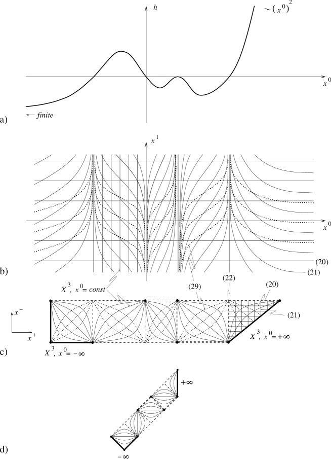
Figure 6.3: Construction of the fundamental building block for a fictitious function $h(x^{0})$. In (b) and part of (c) the null-extremals (6.5), (6.6) are drawn; in the final building block (d) they would run under $\pm 45$ degrees, but have been omitted. In (c),(d) the horizons (6.7) have been drawn as dashed lines (degenerate ones as multiply dashed lines). There and in the Carter-Penrose diagrams we have also included the Killing trajectories (= lines of constant $\phi\equiv X^{3}$), which in (b) have been the straight lines $x^{0}=const$, as thin solid lines. The function $\phi$, and simultaneously $x^{0}$, increases monotonically throughout the block and the ‘boundary’ values of $\phi$ are written to the corresponding boundary segments. Finally, in (b),(c) we have drawn the special extremals (6.13), which are simultaneously the possible flip-axes for the extension.

Figure 6.4: Illustration of relative blue-shift.

The situation becomes particularly drastic if $h(x^{0})$ has zeros of different order as, e.g., in the example chosen in Fig. 6.4 (cf also Fig. 6.3 and the examples R3,4, 7,10 in section 6.1.6): Let $A$ and $B$ be null-extremals leaving the building block across a degenerate (double zero of $h$) resp. nondegenerate horizon as shown in Fig. 6.4. In the chart (5.5) they are described by equation (6.6) and as their affine distance to the horizon we may choose $\tau_{A}:=a-x^{0}$ and $\tau_{B}:=b-x^{0}$. The conformity of the building block requires that a chosen spacing along the null-extremal $A$ transfers to the extremal $B$ via the family of perpendicular null-extremals (6.5), i.e. the lines $x^{1}$ or $v=const$, (cf Fig. 6.4). Now, near the horizon the extremal $A$ may be described asymptotically by $x^{1}\sim 1/\tau_{A}$ and $B$ by $x^{1}\sim-\ln\tau_{B}$, hence $\tau_{B}\sim e^{-1/\tau_{A}}$. When approaching the horizons $\tau_{A}$ and $\tau_{B}$ vanish simultaneously, but also ${d\tau_{B}\over d\tau_{A}}\rightarrow 0$. This already impedes a smooth diagram, which is seen as follows: Choose a conformal gauge (5.3) and let $A$ and $B$ be represented by $u=const=u_{A}$ or $u_{B}$, resp. The affine parameter along these null-extremals then satisfies $d\tau_{A}/dv\propto\exp(\rho(u_{A},v))$ and likewise for $B$, as is easily shown. But from the above we know that at the horizons

$${d\tau_{B}\over d\tau_{A}}={d\tau_{B}/dv\over d\tau_{A}/dv}\propto{\exp(\rho(u_{B},v))\over\exp(\rho(u_{A},v))}\rightarrow 0\,.$$

Thus the conformal factor $\exp(\rho(u,v))$ will either diverge along $A$ when approaching the horizon or, if rendered finite along $A$, vanish along $B$. It is thus impossible to draw a smooth Carter-Penrose diagram in this case! A physical consequence of this is that an observer $B$ approaching the horizon, watching $A$ approaching the degenerate horizon (both observers may also be timelike), will notice that $A$ becomes infinitely blue-shifted. Similar problems occur for any combination of different horizons, only if all horizons are of equal degree the diagram will be smooth.

Nevertheless, it is still possible and instructive to use such ‘nonsmooth Carter-Penrose diagrams’ for book-keeping when constructing the extension and for studying the causal structure. In the illustrations Fig. 6.12, 6.14 we have marked those nonsmooth diagrams with the sign $\bigtriangledown\mbox{\scriptsize!}$ . At any rate, the extended solutions themselves will be smooth.

But even for only nondegenerate horizons there may occur problems, if two triangular sectors meet. While for one sector the boundary can always be made straight by a conformal diffeomorphism, this may be impossible for two adjacent sectors simultaneously: Any conformal diffeomorphism (which is a reparameterization of each of the two lightcone-coordinates $x^{+},x^{-}$) alters the angles between boundary and horizon on both sides of the horizon in the same sense; more precisely, the ratio of the tangents of the respective angles is invariant.

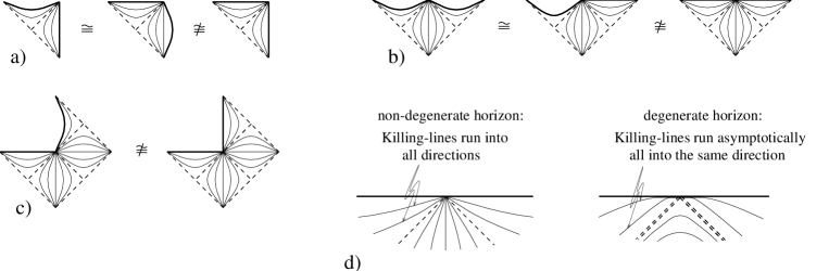
Figure 6.5: Distorted Carter-Penrose-diagrams.

For instance, in the situation of Fig. 6.5a, a conformal diffeomorphism which makes the upper boundary straight must necessarily bulge out the right boundary (at least near the corner point), so the angles of the boundaries against the horizon can never be made equal. This argument is also valid for the (already ‘extended’) diagram Fig. 6.5c, and for similar reasons the angle in Fig. 6.5b cannot be smoothed. At the end of section 6.1.5 (cf Fig. 6.8) we will show by an example that the distorted diagram is in fact the generic case, if two ‘triangular’ sectors meet.

Finally, for degenerate horizons of equal degree these distortions do not occur; one can always obtain right angles or straight lines. But also the Killing lines behave differently then: As can be shown easily using (5.5), (6.5), (6.6) they no longer run from the corner point of the sector in all directions; instead they leave the corner point in only one direction asymptotically (tangential to the boundary, if there is one; cf Fig. 6.5d). This feature applies also to (4d) extremal Reissner-Nordström with its degenerate horizons, which is in this respect drawn incorrectly in most textbooks (e.g. [117]). But also the other issues illustrated by Figs. 6.5 and 6.6 are usually ignored in the literature.

6.1.5 Maximal Extension and Saddle-Point Charts

In the previous section we have compressed the coordinate patches (5.5) into finite building blocks. Now we will investigate whether these blocks have to be extended and how to do so.

Let us again examine the cases without zeros of $h$ first. Their building blocks are drawn in Fig. 6.2 and they are already inextendible, which is seen as follows: If an extension were possible at all, then it must be possible (also) along the null-infinities (i.e., the 45-degree boundaries of Fig. 6.2a,b) or along the timelike (for $h>0$) singularities (the vertical resp. curved boundaries in Fig. 6.2b,c). The extension cannot be possible over a corner point alone, since this point then cannot be an interior point of a new local chart.

Now, if $x^{0}$ ranges over all of I R, then these boundary lines lie at infinite distance since $x^{0}$ is an affine parameter for the null-extremals (6.5, 6.6). Thus they cannot be regular interior points and the solution is inextendible. Note, however, that in general null- and nonnull extremals may have different completeness properties! The completeness of the null-extremals depends on the domain of $x^{0}$, whereas the completeness of the other extremals hinges largely on the (asymptotic) behavior of the function $h$ (cf equation (6.11)). E.g., the boundaries for the $R^{2}$–model (2.6) are ‘null-complete’ (as $x^{0}\in\mbox{{\sl I R}}$) but ‘nonnull incomplete’ (as $\lim_{x^{0}\to\pm\infty}s=$ finite, cf (6.11)). Usually a boundary point is called complete only if all extremals running into it are complete. On the other hand, one complete extremal is sufficient to make the metric inextendible through that boundary point.

If $x^{0}$ does not range over all of I R, then the null-extremals are incomplete and perhaps also the other extremals. However, even then the solution is inextendible, since on these boundaries some physical field ($\phi$ or some dilaton field) diverges. Of course, if these fields are not taken seriously (or if one drops the restriction ${\bf{U}}^{\prime}(\Phi)\neq 0$, requiring it locally only), then one might try to extend the function $h(x^{0})$ smoothly or analytically beyond its original domain and repeat the analysis with this new $h$ to obtain an extension.

In the case where $h$ has zeros, the discussion above is still valid for the first and the last sector, i.e., an extension is not possible beyond those boundary lines. However, at the other, interior, boundary lines the solutions are extendible and this can be done as follows: Already in section 6.1.2.1 we have introduced the flip transformation (6.2). In the Carter-Penrose diagrams this flip shows as a reflexion of the sector in question. The reflexion axis, running diagonally through the sector, has to be transversal to the Killing lines (i.e. horizontal for stationary sectors and vertical for homogeneous ones; cf e.g.  the dotted lines in Fig. 6.3c). The flip transformation breaks down at the horizons bounding the sector, because it maps the interior horizons onto exterior ones. We can, however, flip (i.e. reflect) the whole building block and thus obtain an extension beyond the previously ‘exterior’ horizons. The gluing thus amounts to taking the mirror image of the block and patching the corresponding sectors together. This procedure has to be performed at each sector of the first building block and after that also at each sector of the new building blocks and so on (cf Fig. 6.6 for the first steps).

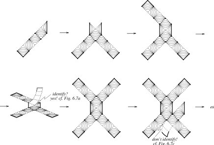
Figure 6.6: The gluing procedure.

This gluing process is essentially unique; the only free parameter is the choice of the symmetry axis of the flip transformation (i.e. the choice of the constant in (5.8)), but it only results in a coordinate change (shifting the $x^{1}$-origin of the charts (5.5)). As long as only the universal covering is pursued this does not affect the solution. However, when further identifications of sectors are made, such that the resulting solution is not simply connected, then we can have an effect of this parameter (this will be discussed in section 6.2).

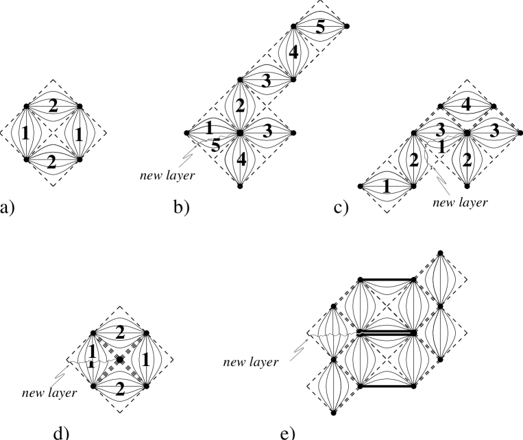
Figure 6.7: Gluing around a vertex point. Only in (a) the four sectors make up a single sheet around the vertex point. In all other cases (b–d) the vertex point is not an interior point and the solutions must be extended into further new layers covering the original sectors. The same is true for the general situation of e.g. (e), showing part of the extended diagram G7 (cf Fig. 6.14).

We have yet to investigate the case (see Figs. 6.6) and (6.7) that after surrounding the point at the vertex of four blocks the overlapping sectors of the first and the fourth block match. Shall they be identified?

This depends: There is exactly one case where they must be identified (Fig. 6.7a) and there are a couple of cases where they could (but shall not). A necessary requirement is of course that the sectors are equal (i.e. isometric, fields like $\phi$ coincide). This is the case in (a),(d) of Fig. 6.7, but generically not in (b),(c), because there different sectors overlap (e.g. in (b) the sectors 1 and 5, if numbered consecutively in the building block); only under rare circumstances (e.g. periodic functions $h$ and $\phi$) they could happen to fit onto one another.

Now to the question whether they shall: If the solution can be extended smoothly into the vertex point, then of course this must be done, and in this case the overlapping sectors have to be identified to make a single sheet around this vertex point (as shown below this will be the case precisely in the situation Fig. 6.7a). If, on the other hand, the vertex point turns out to lie at infinite affine distance, then it cannot possibly be an interior point. If the sectors were identified, then one would have a noncontractible loop around this vertex point, which cannot be accepted since we intend to construct the (simply connected) universal covering. Thus we must not identify the overlapping sectors but start a ‘new layer” and continue the gluing, giving rise to the winding-staircase like structure outlined in Fig. 6.7b–d (cf also Fig. 6.12/R2 or Fig. 6.14 G4). This applies also to the situation (Fig. 6.7e) that a whole slit is surrounded before overlapping, or even more generally to any occurence of overlapping sectors different from the arrangement Fig. 6.7a. Certainly, even if we identify the sectors we still have a (multiply connected) solution of the equations of motion. However, this gluing process is not unambiguous but introduces a (geometrically meaningful) parameter. We will analyze those solutions in all detail in section 6.2.

Our considerations on the completeness of the horizons (cf the paragraph below (6.7)) show already that Fig. 6.7a is the only candidate for a regular vertex point: Degenerate horizons are complete in both directions, whereas nondeg. horizons are complete on one side only, which is easily recognized as that side of the building block where the Killing lines converge (in Fig. 6.7 all such complete points have been marked by massive dots). But even the general extremals running towards those vertex points show the same behavior: Those running along with converging Killing-lines into the vertex point are either oscillating ones (between two fixed $\phi$– resp. $x^{0}$–values, cf (6.9)) or of the kind (6.10), which are both complete. And those running transversally to the Killing lines are precisely those of (6.9) with $c=0$, i.e.,

$${dx^{1}\over dx^{0}}=-{1\over h},$$ (6.13)

and coincide, furthermore, with the possible symmetry axes for the flip transformations (in Fig. 6.3b,c we have drawn some of them as dotted lines). Their length follows from (6.11) where $a$ is the zero of $h(x^{0})$ in question:

$$s=\int^{a}{dx^{0}\over\sqrt{|h|}}\sim\int^{a}{dx^{0}\over{(x^{0}-a)^{n\over 2}}}\to\left\{\begin{array}[]{r@{\quad}l}<\infty&n=1\\ \infty&n\geq 2\end{array}\right.\quad.$$ (6.14)

It is finite only at simple zeros. Thus, whenever a degenerate horizon runs into the vertex point or Killing lines focus there, then this vertex point is at infinite distance and has to be taken out of consideration. In these cases, to obtain the universal covering we must not identify the overlapping sectors but continue the gluing in a new layer.

In the case of Fig. 6.7a (only nondeg. horizons and the Killing lines avoiding the vertex point), however, all extremals are incomplete, and it is thus to be expected that the vertex point is a regular interior point of the manifold. This is indeed true: equation (5.51) represents a smooth nondegenerate metric for the neighbourhood of such points, which reveals the vertex point as regular interior point (a saddle point of $\phi$, with $X^{a}=0$). The four adjacent sectors then constitute one single sheet (cf also diagrams 3–5 of Fig. 6.6).

Keeping in mind the Schwarzschild-like form of (5.6), there is also an alternative way of obtaining such a saddle-point chart, imitating the Kruskal-Szekeres procedure. It was initially proposed by M. Walker [114] for a special rational form of $h$. We want to show here that it works for any sufficiently smooth $h$ (say $C^{n}$) with simple zero at $x^{0}=a$. The transformation reads (with $f$ as in (5.8))

$$u=\hbox{sgn}(h)\exp{h^{\prime}(a)\left[f(x^{0})+\frac{x^{1}}{\scriptstyle 2}\right]}=\hbox{sgn}(h)\exp{\int\limits^{\,\,\,\,x^{0}}\!\!\frac{\scriptstyle h^{\prime}(a)}{\scriptstyle h(x)}dx+\frac{\scriptstyle h^{\prime}(a)}{\scriptstyle 2}x^{1}}$$ (6.15)

$$v=\exp{-\frac{\scriptstyle h^{\prime}(a)}{\scriptstyle 2}x^{1}}\,\,.$$ (6.16)

It brings the metric (5.5) into the form

$$ds^{2}=-\frac{4\widetilde{h}(uv)}{h^{\prime}(a)^{2}}\frac{dudv}{uv}\,,$$ (6.17)

which is evidently nonsingular and nondegenerate around $u,v=0$. Here $\widetilde{h}(uv)$ is determined implicitly via $\widetilde{h}(uv)=h(x^{0}(u,v))$. The integration constant hidden in $u$ has to be chosen such that $u$ is continuous at $x^{0}=a$.

To show that the transformation (6.15), (6.16) is really a (local) diffeomorphism consider the following decomposition of the integrand in (6.15) (separating the singular term):

$$\frac{h^{\prime}(a)}{h(x)}=\frac{1}{x-a}-\frac{\frac{h(x)}{x-a}-h^{\prime}(a)}{h(x)}\,\,.$$ (6.18)

The first term yields (after integration and exponentiation) a factor $(x-a)$, and also the second term (being $C^{n-2}$, if $h\in C^{n}$) behaves perfectly well. It is thus not at all necessary that $h$ is of the special rational form given in [114, 115].

We are now finally in the position of proving the statement on the distorted boundary of the $R^{2}$–gravity solutions made at the end of section 6.1.4. Let e.g. $\Lambda=-{1\over 3},C={4\over 3}$, hence (cf equation ((5.13)) $h={2\over 3}\left[2-x^{0}-(x^{0})^{3}\right]$. Equations (6.15), (6.16) can be integrated easily to

$$uv = \mbox{sgn}(h)\exp\int\limits^{\,\,\,\,x^{0}}{{h^{\prime}(1)}\over{h(x)}}dx=$$ (6.19)

$$= \mbox{sgn}(h)\sqrt[8]{(x^{0})^{2}-2x^{0}+1\over(x^{0})^{2}+x^{0}+2}\exp\left({{-3\over 4\sqrt{7}}\arctan{1+2x^{0}\over\sqrt{7}}}\right)\,\,.$$

The singularities lie at $x^{0}=\pm\infty$, i.e. at $uv=\exp\left(-{3\pi\over 8\sqrt{7}}\right)\approx 1.561$ and $uv=-\exp\left(+{3\pi\over 8\sqrt{7}}\right)\approx-0.641$, respectively.

Figure 6.8: Distorted Carter-Penrose-diagrams for the $R^{2}$–model.

The familiar conformal diffeomorphism $u\rightarrow\tan\hat{u},v\rightarrow\tan\hat{v}$ shows immediately that the correct shape of the Carter-Penrose diagram must be like in Fig. 6.8b,c (it is of course possible to straighten the one boundary line at the cost of the other by means of conformal diffeomorphisms). Only if the two hyperbolae $x^{0}=\pm\infty$ happen to lie at equal values of $|uv|$ then we can obtain a square. Thus for nonsymmetric functions $h$ (with one zero) squares are rather the exception to the rule. This remark applies also to the square shaped Carter-Penrose diagrams obtained, e.g., in [115, 121] for other special models covered by the present treatment. Finally we want to mention some physical difference between a world with a square-shaped Carter-Penrose diagram and another of the generic form Fig. 6.8b,c: Only in the former case a series of null-lines ‘bouncing off’ the boundaries closes to a rectangle (cf dotted lines in Fig. 6.8).

6.1.6 Recipe and examples

Let us summarize briefly the principle of how to construct the maximally extended Carter-Penrose diagram corresponding to any function $h$ in (5.5):
$\bullet$ The number and kind of zeros of the function $h$ determines the number of sectors and their ‘orientation’ in a fundamental building block ($h>0$ corresponds to stationary sectors, $h<0$ to homogeneous ones). More explicitly: For $n$ zeros of $h$ there are $n+1$ sectors in the building block. If a zero of $h$ is of odd order, then the corresponding Killing horizon separates a stationary from a homogeneous sector; otherwise the two neighboring sectors are clearly of the same type (as $h$ does not change its sign).
$\bullet$ The end sectors of the building block are either a square or a triangle, depending on the asymptotic behavior of $h$. It is a triangle, if $f(x^{0})=\int^{x^{0}}du/h(u)$ remains finite at the boundary (e.g., for $h(x^{0})\sim(x^{0})^{k>1}$ as $x^{0}\to\pm\infty$), and it is a square, if $f(x^{0})$ diverges (e.g., for $h(x^{0})\sim(x^{0})^{k\leq 1}$ as $x^{0}\to\pm\infty$).
$\bullet$ Choose any sector and establish the symmetry axis, running diagonally through the sector, transversal to the Killing lines (i.e. horizontal for stationary sectors and vertical for homogeneous ones). Reflect the whole block at this symmetry axis and identify the corresponding sectors.
$\bullet$ Proceed in this way with all sectors until you come to an end, or ad infinitum.
$\bullet$ If after surrounding a vertex point sectors overlap, the Killing horizons running into that point being nondegenerate (simple zero of $h$), and if the Killing lines do not focus in that point (Fig. 6.7a), then identify the overlapping sectors such as to make a single sheet around this vertex point. In all other cases (e.g. higher degree zero of $h$, Killing-lines running into that point, etc.) do not identify the sectors, but continue gluing in a new layer to get the universal covering.
$\bullet$ Any boundary is null-complete, iff $x^{0}\to\pm\infty$ there. A boundary point is complete with respect to all other extremals (6.9), iff $\int^{x^{0}}du/\sqrt{|c-h(u)|}$ diverges there, (cf equation (6.11)). Complete boundaries have to satisfy both conditions (except that only extremals of one kind run there) and are depicted boldfaced.

As pointed out repeatedly before, the Carter-Penrose diagrams obtained in this way are to be understood as schematic ones only. However, if the zeros of the respective function $h$ are all of the same order, then these diagrams are also smooth. By this we mean that there exists a (smooth) diffeomorphism from the universal covering solution to the respective diagram, so that the diagram may indeed be regarded as a chart to the spacetime (cf our discussion in section 6.1.2). Still, if the zeros are all simple (nondegenerate horizons) and two nonnull boundary lines meet in a point, then it will in general be necessary to deform the boundary lines somewhat (cf Figs. 6.5a–c, 6.8). For a null and a nonnull boundary line meeting or for higher order zeros these complications do not occur.

If, on the other hand, $h$ has zeros of different degree, then there is no smooth diffeomorphism from the universal covering solution to the Carter-Penrose diagram; the latter has to be regarded as purely schematic then. An explanation from the physical point of view has been provided by means of a relative red/blue-shift between observers approaching Killing horizons of a different type (cf Fig. 6.5). Certainly the universal covering solutions themselves are still smooth everywhere in these cases, too: The gluing diffeomorphism (6.2) may be used to patch together charts (5.5) (this poses no problem since only one kind of Killing horizon at a time is involved) and an atlas is obtained when completing these charts by those of type (5.51) or (6.17). Obviously, also in these cases it is instructive to keep track of the patching by a (schematic Carter-Penrose) diagram; only it may not be taken as a true smooth image of the respective spacetime then.

We now come to the announced examples, starting with (anti-)deSitter gravity (3.21). Since all values $\Lambda\neq 0$ yield (basically) equivalent Carter-Penrose diagrams, we will set $\Lambda:=-2$ in the following. This describes deSitter gravity. For positive values of $\Lambda$ (anti-deSitter gravity) the Carter-Penrose diagrams obtained below have to be turned by an angle of 90 degrees, while $\Lambda=0$ yields the diamond like Minkowski space diagrams, of course. We then get a one-parameter family of functions $h$ [cf equation (5.12)], $h^{JT}(x^{0})=C-(x^{0})^{2}$, parameterized by the Casimir constant $C=X_{a}X^{a}+(\phi)^{2}$ (cf Fig. 6.9).

Figure 6.9: Functions $h(x^{0})$ for the JT–model.

J1: For any $C>0$ this curve $h(x^{0})$ has two simple zeros, leading to one square within the fundamental building block. Asymptotically we have $h\sim-{(x^{0})}^{2}$, so that adjacent to the square there will be a triangle at each side, the boundary of which, $\phi=\pm\infty$ resp., is spacelike and complete. Gluing leads to the ribbon-like diagram shown in Fig. 6.10. (For the other sign of the cosmological constant, e.g. $\Lambda=+2$, we get the same diagram for $C<0$, rotated, however, by 90 degrees, as the infinity is timelike then).

J2: For $C=0$ we get no square, but only two triangles. The corresponding Carter-Penrose diagram is again plotted in Fig. 6.10.

J3: For $C<0$ the function $h$ has no zeros (Fig. 6.9). We therefore may apply directly the diffeomorphism (6.12) with the function (5.8), which in the present case can be written in terms of elementary functions:

$$f(x^{0})=-{2\over\sqrt{-C}}\arctan\left({x^{0}\over\sqrt{-C}}\right)\,.$$ (6.20)

The resulting region $(x^{+},x^{-})$ is again a ribbon (Fig. 6.10); but this time without such a periodic internal structure as before, since the Killing lines $\phi=x^{0}=const$ become the parallels $x^{+}-x^{-}=const$ in the present case.

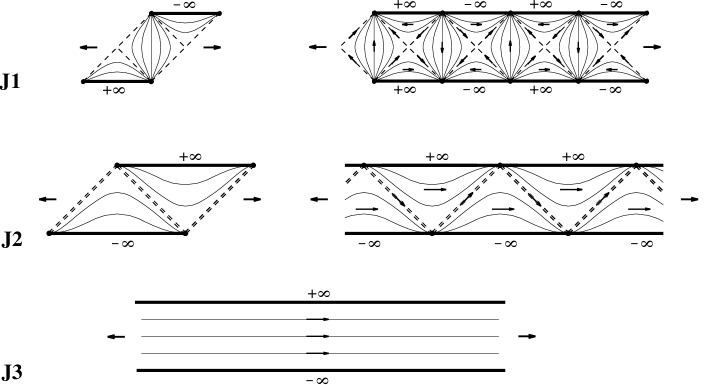
Figure 6.10: Carter-Penrose diagrams for the JT–model; left the building blocks, right the extended diagrams. Arrows inside the diagrams indicate Killing fields for those solutions.

Clearly, as manifolds the solutions J1-3 are all the same, namely the unique (simply connected, maximally extended) manifold with zero torsion and constant curvature ($R\equiv\Lambda$, cf equation (3.21)). The difference between the spacetimes J1-3 arises only from the function $\phi$ defined on them. Preservation of $\phi$ reduces the originally three independent Killing-fields to only one symmetry direction (indicated by arrows in Fig. 6.10).

Note that while the Carter-Penrose diagrams for anti-deSitter space coincide for all dimensions (vertical ribbon), they apparently differ for deSitter space: D-dimensional deSitter space can be obtained from restricting a $D+1$-dimensional Minkowski metric to the one-sheet hyperboloid, the topology of which is $\mbox{{\sl I R}}\times S^{D-1}$. In particular, this hyperboloid is simply connected for $D>2$ and thus yields already the universal covering space. Also, upon spherical reduction, its Carter-Penrose diagram is the familiar square [117]. For $D=2$, on the other hand, this hyperboloid is topologically a cylinder $\mbox{{\sl I R}}\times S^{1}$ and the universal covering, obtained by unwrapping the $S^{1}$ to I R, is clearly the horizontal ribbon of Fig. 6.10. Thus for $D=2$ (and only there) deSitter and anti-deSitter space are related by a simple signature change and the corresponding Carter-Penrose diagrams are just rotated by 90 degrees against one another.

Let us now turn to the second example: $R^{2}$–gravity (2.6). The corresponding function $h(x^{0})$ is in this case [cf equation (5.13)] $h^{R^{2}}=-\frac{2}{3}(x^{0})^{3}+2\Lambda x^{0}+C$. Since $x^{0}$ ranges over all of I R and at infinity $h\sim(x^{0})^{3}$ we get incomplete (null-complete but nonnull-incomplete) triangular sectors at both ends of the building block. The corner points are, however, complete, since only the null extremals (6.7) run into them. A more detailed analysis yields five qualitatively different cases depending on the parameters $C$ and $\Lambda$ (see Fig. 6.11):

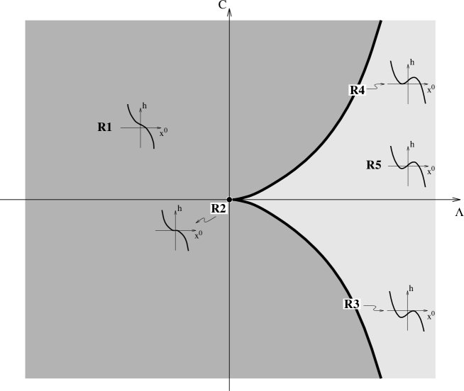
Figure 6.11: $R^{2}$–gravity, overview.

R1 :	one simple zero of $h$ at $x^{0}=B$
R2 :	one triple zero at 0
R3 :	one simple zero at $B_{1}$ and one double zero at $+\sqrt{\Lambda}$
R4 :	one double zero at $-\sqrt{\Lambda}$ and one simple zero at $B_{3}$
R5 :	three simple zeros at $B_{1}$, $B_{2}$, and $B_{3}$,

where $B_{1}<-\sqrt{\Lambda}<B_{2}<+\sqrt{\Lambda}<B_{3}$ and $-\infty<B<+\infty$. Obviously ${\phi}_{crit}=\pm\sqrt{\Lambda}$ (by its definition as zero of the potential $W(0,\phi)$) and the curve along R4,2,3 in Fig. 6.11 corresponds to the critical values $C_{crit}\equiv\pm(4/3)\Lambda^{(3/2)}$ of $C$. It is completely straightforward to construct the Carter-Penrose diagrams according to the above rules. The result is depicted in Fig. 6.12. Note that not only R2 but also the extended solutions R3-5 will be multi-layered; for instance, the copies appended to R4 at the upper left and the upper right horizon, resp., lie in different layers of the universal covering (cf Fig. 6.7e for a similar situation). For nonnegative $\Lambda$ there are, in addition to those diagrams, also infinite ribbons for the constant curvature solutions $d\omega=\mp 2\sqrt{\Lambda}\varepsilon$ (cf equation (5.54)); in the diagram Fig. 6.11 they are located at the curve R4,2,3, i.e. at $C=C_{crit}(\Lambda)$.

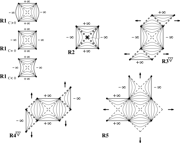
Figure 6.12: Carter-Penrose diagrams for the $R^{2}$–model. Those marked $\bigtriangledown\mbox{\scriptsize!}$   are nonsmooth; furthermore, the singularities of R5 might be distorted in the same way as sketched in Fig. 6.5c. (For more details cf caption of Fig. 6.14).

So, for a negative cosmological constant $\Lambda$, which in contrast to $C$ is fixed by the choice of the action (2.6), there is only one schematic Carter-Penrose diagram (cf Fig. 6.11). The choice of the one free parameter $C$, however, influences the causal structure of R1 somewhat, giving rise to the distorted boundaries (cf also Fig. 6.8). For positive values of $\Lambda$ there are mainly two kinds of (again schematic) Carter-Penrose diagrams: R1 and the a bit more complicated diagram R5. Again, to have them smooth, some of the boundaries will be curved for generic values of $C$ (also for R5, although this has not been indicated in Fig. 6.11!). The separation of the solution space into solutions of the type R1 and R5 occurs at the values $\pm(4/3)\Lambda^{(3/2)}$ of $C$. At these values we have the spacetimes corresponding to the (inherently nonsmooth) Penrose diagrams R3,4 and those of deSitter type with $R\equiv\pm 4\sqrt{\Lambda}$ (but now with no internal structure as the functions $X^{i}$ are constant all over $M$ here). So at $C=C_{crit}$ the Casimir constant does no longer classify the universal coverings uniquely. This is related to the fact that there is more than one symplectic leaf for a critical value of $C$: Besides a two-dimensional leaf, corresponding to R4 resp. R3, there is the pointlike one $X^{+}=X^{-}=0$, $\phi=\phi_{crit}$, corresponding to a deSitter solution of positive resp.  negative constant curvature.

The third example is the Katanaev-Volovich model (2.17). Its function is $h^{KV}(x^{0})={1\over\alpha}\left\{Cx^{0}-2(x^{0})^{2}[(\ln x^{0}-1)^{2}+1-\Lambda]\right\}\,,$ where $x^{0}\in\mbox{{\sl I R}}^{+}$. The function $h^{KV}$ always has a zero at $x^{0}=0\Leftrightarrow\alpha\phi=-\infty$, which is at least of order one. Thus the function $f=\int^{x^{0}}du/h(u)$ (cf equation (5.8)) has infinite range as $x^{0}\to 0$, which shows that the Carter-Penrose diagrams have a square-shaped sector at this end, the null-infinities, however, being incomplete. On the other boundary of the coordinate patch, $\alpha\phi=+\infty$, we find $\alpha h\sim(x^{0})^{2}\ln^{2}x^{0}$, corresponding to a complete triangular sector at this end.

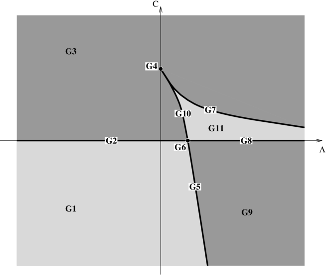
Figure 6.13: KV–model, overview. The different regions correspond to qualitatively different functions $h$ (number and degree of zeros, asymptotic behavior at 0 and $+\infty$).

This time we get 11 qualitatively different cases (in addition to two deSitter solutions) depending on the parameters $C$ and $\Lambda$:

G1,2 :	no zeros of $h$
G3 :	one simple zero at $x^{0}=B$
G4 :	one triple zero at $x^{0}=1$
G5,6 :	one double zero at $x^{0}=e^{\sqrt{\Lambda}}$
G7 :	one double zero at $e^{-\sqrt{\Lambda}}$ and one simple zero at $B_{1}$
G8,9 :	two simple zeros at $B_{2}$ and $B_{1}$
G10 :	one simple zero at $B_{3}$ and one double zero at $e^{\sqrt{\Lambda}}$
G11 :	three simple zeros at $B_{3}$, $B_{2}$, and $B_{1}$,

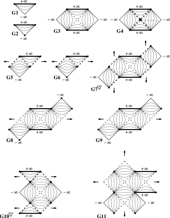
Figure 6.14: Carter-Penrose diagrams for the KV–model (those marked $\bigtriangledown\mbox{\scriptsize!}$   are nonsmooth!). Complete boundary lines are indicated by boldfaced lines, complete points (points at infinity) by massive dots, incomplete boundary lines by thin solid lines, and horizons by dashed lines (degenerate horizons, i.e. at higher order zeros of $h$, by multiply dashed lines). The null extremals (6.5, 6.6) which run through the diagrams under $\pm 45$ degrees are omitted. Arrows outside a diagram (G5-11) indicate that the solution should be extended by appending similar copies at the corresponding boundaries (but cf Fig. 6.7e).

where $0<B_{3}<-\sqrt{\Lambda}<B_{2}<+\sqrt{\Lambda}<B_{1}$ and $B\in\mbox{{\sl I R}}^{+}$. An overview is provided by Fig. 6.13. In the above list we took $x^{0}\in\mbox{{\sl I R}}^{+}$. The cases G2,6,8 and G1,5,9, respectively, differ only in the asymptotic behavior of $h$ at $x^{0}\rightarrow 0$ ($h^{KV}\sim x^{0}$ for $C\neq 0$, but $h^{KV}\sim(x^{0}\ln x^{0})^{2}$ for $C=0$), which influences the completeness properties (see below). The critical values of $\phi$ are easily determined to be $\pm\sqrt{\Lambda}/\alpha$; the corresponding value of the Casimir function $C$ is

$$C_{crit}=-4\left(\pm\sqrt{\Lambda}-1\right)\exp\left(\pm\sqrt{\Lambda}\right)\,,$$ (6.21)

which marks the curve G5,6,10,4,7 of Fig. 6.13 and simultaneously the deSitter solutions $De^{a}=0,\,d\omega=\pm{2\over\alpha}\sqrt{\Lambda}\varepsilon$ (cf equation (5.54)).

It is now straightforward to draw the Carter-Penrose diagrams of the KV–model. The result for $\alpha>0$ is depicted in Fig. 6.14 (extended versions of G5,9 are given in Fig. 6.15); the diagrams for $\alpha<0$ are obtained by rotating these by $90$ degrees. According to the different behavior of $h$ at the boundary $x^{0}=0$ the Carter-Penrose diagrams G2,6,8 ($C=0$) differ from G1,5,9, respectively, only by having a complete time–(space–)infinity, $\alpha>\!(<)\,0$, at that boundary (use (6.11)). Let us stress that all Carter-Penrose diagrams in Fig. 6.14 except for G7,10 are smooth now, the boundary lines being actually straight (cf previous footnote). Again, however, a representation of the extended diagrams for G4,7,10,11 will require infinitely many overlapping layers (cf Fig. 6.7e for the case G7).

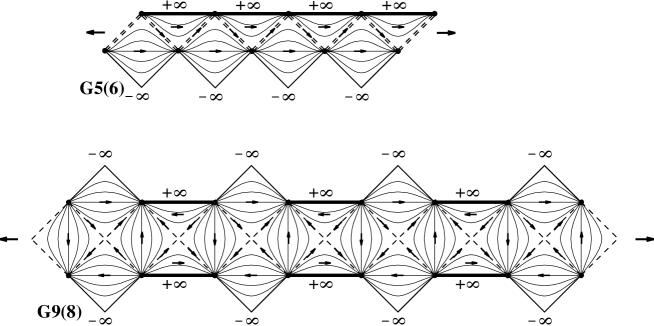
Figure 6.15: Some extended Carter-Penrose diagrams for the KV–model. Arrows inside the diagrams indicate Killing fields.

The numbering G1-11 has been chosen as in [122], where the Carter-Penrose diagrams Fig. 6.14 have been constructed first. It should be noted, however, that our procedure to obtain these diagrams is incomparably faster than the one of [122]. The main reason is that the local solutions used there (resulting also from ours through the diffeomorphism (6.12)) are valid only in coordinate patches which are part of ours (the sectors $h(x^{0})\neq 0$); they had to be glued along their border, which entailed lengthy considerations of the asymptotic behavior. In the chiral gauge (5.5), instead, the charts overlap and simply have to be matched together. As a consequence we also could prove that all the solutions of (2.17), (and in fact also of (2.19) with an, e.g., analytic potential $W$) are analytic. As pointed out repeatedly, the Carter-Penrose diagrams G7,10 are, however, not smooth but have to be regarded as schematic diagrams only (of course, the universal covering solutions themselves are smooth).

As a further example for the application of the simple rules outlined at the beginning of this subsection we could consider, e.g., a model (5.1) where $V$ is chosen to be the derivative of our generic function $h$ in Fig. 6.3a. In this torsion-free case with $g=2e^{+}e^{-}$, the function $h$ in (5.5) will coincide with the function in Fig. 6.3a up to a ‘vertical’ shift according to (5.12). It is now not difficult to see that there will be 11 qualitatively different schematic Carter-Penrose diagrams in this case, as well as further four deSitter solutions (corresponding to the four distinct extrema of the function $h$ in Fig. 6.3a or, equivalently, to the four zeros of the potential $V$). We leave it as an exercise for the interested reader to sketch these Carter-Penrose diagrams explicitly. Note that some of them will be quite ramified already (cf, e.g., Fig. 6.6), a feature that becomes more and more pronounced with an increasing number of zeros of $V$ (or $h$).

This completes our analysis of the universal coverings of a general pure gravity (or gravity–YM) model. Starting from any of these Lagrangians, the determination of the corresponding Carter-Penrose diagrams is straightforward now. One just has to determine the function $h$ as, e.g., in (5.12). Thereafter the coverings follow from simple rules where only the zeros of $h$ and its asymptotic behavior enters. This was illustrated by several examples above. As remarked already before, the procedure is applicable also to the analytic extension of any metric with a Killing field (cf the remarks in section 6.1.1).

6.1.7 Remarks on global coordinates

For many of the Carter-Penrose diagrams, such as e.g. for R1,G3,5,9, it is possible to find also global coordinates, displaying explicitly the analyticity of the metric. E.g., for R1,G3 we have already found the Kruskal-like coordinates (6.17) or the more explicit ones (5.51), and instead of for G5,9 we provided a global, explicitly analytic chart in a chiral gauge (5.4) for the (mathematically) quite similar (four-dimensional) Reissner-Nordström solution in [123]. The method presented there may be adapted easily to cases such as G5,9 or in fact to any two-dimensional spacetime with a Killing field that permits a foliation by null-lines.

The main idea of [123] is that in such cases there is no Gribov obstruction [124] to picking the light cone gauge (5.4) or (5.18). Thus there must exist functions $F$ and $G$ in (5.20) yielding a globally well–defined solution. The residual gauge freedom of (5.18) may then be used to simplify these two functions. The resulting problem for $F$ may be mapped to the problem of classifying vector fields on a line modulo diffeomorphisms; the number of zeros of $F$ is thus gauge invariant, among others. The field equations pose restrictions on the slope of $F$ at its zeros. For the case of SS or RN, e.g., the residual gauge freedom may be used to bring $F$ (and also $G$) into a form containing elementary functions only. E.g., for SS $F\propto x^{1}$ and $G=const$ may be achieved, while for RN $F$ and $G$ may be fixed by using $\cos$ and $\sin$. (Cf [123] for the details).

For SS the resulting coordinates provide a hardly known, explicit global chart (found first by [125]) as an to interesting alternative to the much better known Kruskal coordinates [126]. The method provides also an explicit analytical global chart for the RN spacetime. Both of these charts should be at least of pedagogical interest.

6.2 All global solutions of (all 2d) Gravity–Yang–Mills models

6.2.1 Introductory remarks

In this section we want to classify all global, diffeomorphism inequivalent classical solutions of a general pure gravity model. In particular the analysis covers the generalized dilaton gravity models (3.15). The classification shall be done without any restriction on the topology of the spacetime $M$.

For some of the popular, but specific choices of the potentials ${\bf{U}},{\bf{V}},{\bf{Z}}$, in (3.15) such as those of string inspired dilaton gravity (section 3.1.2), of deSitter gravity (equation (3.21)), or of spherically reduced gravity (section 3.1.1), the possible topologies of the maximally extended solutions turn out to be restricted considerably through the field equations. In particular their first homotopy is either trivial or (at most) ${{\bf{Z}}}$. (Permitting e.g. also conical singularities, cf section 6.2.5, the fundamental group might become more involved.)

For any ‘sufficiently generic’ (as specified below) smooth/analytic choice of ${\bf{U}},{\bf{V}},{\bf{Z}}$, on the other hand, the field equations of $L$ permit maximally extended, globally smooth/analytic solutions on all noncompact two-surfaces with an arbitrary number of handles (genus) and holes ($\geq 1$). This shall be one of the main results of the present section. These solutions are smooth and maximally extended, more precisely, the boundaries are either at an infinite distance (geodesically complete) or they correspond to true singularities (of the curvature $R$ and/or the dilaton field $\Phi$). We will call such solutions global, as there are other kinds of inextendible solutions (cf below, in particular section 6.2.5).

6.2.1.1 Motivation

The existence of solutions on such nontrivial spacetimes is a qualitatively new challenge for any program of quantizing a gravity theory. Take, e.g., a Hamiltonian approach to quantization: In any dimension $D+1$ of spacetime the Hamiltonian formulation necessarily is restricted to topologies of the form $\Sigma\times R$ where $\Sigma$ is some (usually spacelike) $D$-manifold. In our two-dimensional setting, $\Sigma$ may be I R or $S^{1}$ only. Thus $\pi_{1}(M)$ can be ${{\bf{Z}}}$ at most. According to our discussion above, this is far from exhaustive in most of the models (3.15).

Let us compare this to the case of full four-dimensional Einstein gravity. Clearly, there the space of solutions will include spacetimes of complicated topologies. Therefore, a restriction to topologies of the form $M=\Sigma\times R$ seems hardly satisfactory in the 4d scenario as well. A path integral approach to quantum gravity, on the other hand, does not place an a priori restriction on the topology of the base manifold $M$. However, also in the path integral approach for $M\neq\Sigma\times R$, the definition of an integration measure is plagued by additional ambiguities and problems, cf [128]. The class of models (3.15) (and also the theories with torsion, equation (2.19)) may serve as a good laboratory to improve on that situation and to gain new insights in such directions.

For spacetimes of topology $\Sigma\times R$, furthermore, we are interested in an explicit comparison of the solution space or moduli space of a given action (space of all solutions to the field equations modulo diffeomorphisms) with the reduced phase space (RPS) in a Hamiltonian formulation of the theory. In the simply connected case ($\Sigma=R$) we already classified all global diffeomorphism inequivalent solutions in the previous section. The solution space was found to be one-dimensional, parameterized by a real number $C\in R$. As the result of a symplectic reduction must lead to an even-dimensional RPS, we may conclude that in the case of an ‘open universe’ ($\Sigma=R$) the proper definition of a Hamiltonian system, describing the same physics as (3.15) (or (2.19)), is in need of some additional external input. This seems to creep in implicitly when defining boundary/fall-off conditions for the canonical phase space fields and/or by declaring some particular gauge transformation of the Lagrangian formulation of (3.15) as (nongauge) symmetry transformation (cf also section 7.1 below). Periodic boundary conditions, on the other hand, lead to a Hamiltonian formulation which is perfectly well-defined without any further input besides that of periodicity (with respect to some arbitrarily fixed coordinate period). Effectively they describe the case of a ‘closed universe’ $\Sigma=S^{1}$ and we conclude that for cylindrical topologies of $M$ the solution space of (3.15) must be even-dimensional. Indeed it will turn out to be two-dimensional, a second parameter ‘conjugate to $C$’ arising from the ‘compactification’ (in one coordinate).

For generic 2d gravity theories the solution space for $M\sim S^{1}\times R$, and thus the corresponding RPS, will have a highly nontrivial topology. This is the second challenge which has to be faced in a quantization scheme: One has to cope with this nontriviality of the orbit space, as for sure the RPS of four–dimensional gravity will be even more intricate.

We will come back to these issues in chapter 7. We mentioned them here already as they also serve as part of the interest for the classification performed in the present section.

6.2.1.2 Organization

To classify the global solutions, we will employ three different, alternative methods. First, at the example of the KV model (2.17), solutions of nontrivial topology are obtained from a ‘cut-and-paste’ technique: Starting from the Carter-Penrose diagrams, we cut out some fundamental region and glue it together appropriately. In this process, we keep track of different parameters labeling inequivalent gluings. Together with the Casimir parameter $C$ labeling the Carter-Penrose diagrams, these parameters are coordinates on the moduli space.

Second, we will employ the $\sigma$-model approach of chapter 4 for a direct classification. In the case of pure gravity models it is possible to solve the field equations globally within this framework, for arbitrary topology of $M$. The respective calculation may again be performed within a few lines only. However, per se the PSM formalism does not care about the physical restriction that the metric should be nondegenerate globally. Thus, the solutions obtained will include solutions which have to be excluded on these grounds in a second step. We did not manage to incorporate this restriction in a sufficiently practical way. Therefore, as of present state, the PSM formalism gives an upper bound to the dimension of the moduli space only.

Last but not least a systematic, group theoretical approach will be applied. For that purpose we will determine the full isometry group ${\cal G}$ of the universal covering solutions first. All global solutions may be obtained as factor solutions of the universal coverings by appropriate discrete subgroups of ${\cal G}$. This will yield a complete classification for a general pure gravity model in terms of conjugacy classes of discrete groups. The simple machinery developed will fail, however, for those solutions with three Killing vectors, which describe spaces of constant curvature; they are thus discussed separately (and, although apparently simpler, they are not fully classified yet). In the subsection on the group theoretical approach we will also provide a geometrical interpretation of the additional parameters arising.

In a final subsection, furthermore, we will briefly discuss ‘nonglobal inextendible’ solutions (some remarks on them are found already in section 6.2.2, too). They are connected to so-called kinks (of the metric). For a cylindrical spacetime, for example, the (discrete) kink number of a metric may be defined as follows: It is the minimal number of disconnected null-like parts (or points) of any noncontractable line. Loosely speaking, the light cone tilts around nontrivially along the noncontractable loop. The moduli space then splits into separate, disconnected parts, characterized precisely by the kink number.

6.2.1.3 Anticipation of some of the results

Also the classification of all global solutions will be found to depend solely on the number and order of the zeros of the function $h(r)$ in (5.5) (as well as there asymptotic behavior). To provide an overview on the results, we restrict ourselves to simple zeros $h$ (zeros of higher order occur only for specific values of the parameter $C$).

Besides the uniquely defined universal covering, one obtains the following global space– and time–orientable solutions ($n=\mbox{\# simple zeros of h}$):

• Cylinders labelled by their circumference (real number).

• The above cylinders are still available, but now incomplete in a pathological manner (Taub–NUT space).

• Complete cylinders labelled by a discrete parameter (patch number) and a further real parameter.

• Noncompact surfaces of arbitrary genus with an arbitrary number ($\geq 1$) of holes. The number of continuous parameters equals the rank of the fundamental group $\pi_{1}(\mbox{solution})\equiv\pi_{1}(M)$, and there are also further discrete parameters.

The solution space for a fixed model (2.19) or (3.15) and for a fixed topology is labelled by the above parameters plus the (mass) parameter $C$. For the case of additional YM–fields, its dimension generalizes to $(\mbox{rank }\pi_{1}(M)+1)\,(\mbox{rank (gauge group)}+1)$.

Thus by a ‘sufficiently generic’ generalized dilaton theory at the beginning of the present section 6.2.1, we meant an action characterized by potentials ${\bf{U}},{\bf{V}},{\bf{Z}}$ which, at least for some values of $C$, give rise to a function $h$ with three or more zeros (cf, also, equation (5.12)).

6.2.2 Cut-and-paste technique for the KV model

Figure 6.16: Some Penrose-diagrams for the KV–model. The thin lines denote Killing trajectories, the broken lines Killing horizons. The style of the boundary lines indicates their completeness properties; however, since they are irrelevant for our topological considerations, we will treat them rather sloppily. The arrows in G9 indicate that the patch should be extended horizontally by appending similar copies, and likewise G11 should be extended vertically and horizontally.

In this section we discuss possible global solutions for the Katanaev-Volovich (KV) model (2.17). Its universal covering solutions, resulting from the analysis of the function $h$ in (5.46), were obtained already in section 6.1.6, cf Figs. 6.13 and 6.14. For reasons of brevity we skip the solutions where $h$ has higher order zeros in this section; also we postpone a discussion of the deSitter solutions (section 6.2.4.5). They both occur only for positive $\Lambda$ and only for those two particular values $C_{\pm}(\Lambda)$ of $C$ on the boundary lines between G1/G9 or G3/G11 (i.e. at G4-7,10 in Fig. 6.13)! The remaining, ‘generic’ diagrams are collected in Fig. 6.16.

The KV model is adequate to illustrate much of what has been said in the introductory remarks to this section as well as to get a grasp on the general case. In particular, for a negative cosmological constant $\Lambda$ there are only the simple Carter-Penrose diagrams G1 and G3. Despite some differences, in the present context, the situation for negative $\Lambda$ reminds much of spherically symmetric vacuum gravity: Also there a horizon is present only for positive Schwarzschild mass $m\sim C$ and none for negative values of $M$. Moreover, like the spherical model,the KV–model with $\Lambda<0$ belongs to the class of particular models where the possible topologies of spacetimes are restricted severely.

As mentioned above one obtains all noncompact two-surfaces, if the one-parameter family $h=h_{C}(x^{0})$ contains functions with three or more zeros. In the KV–model this is the case for positive $\Lambda$, where the additional diagrams G11 if $0<\Lambda<1$ as well as G9 if $\Lambda>1$, cf Figs. 6.13, 6.16 arise.

We start with G1: Obviously this is a spatially homogeneous spacetime and (5.5) provides a global chart for it. Identifying $x^{1}$ and $x^{1}+\omega$, $\omega=const$, evidently we obtain an everywhere smooth solution on a cylindrical spacetime $M\sim S^{1}\times R$. It results from the Carter-Penrose diagram G1 by cutting out a (fundamental) region, e.g. the strip between two null-lines in Fig. 6.17, and gluing both sides together in such a way that the values of the curvature scalar $R$, constant along the Killing lines, coincide at the identified ends. The constant $\omega$ (or a function of it) becomes the variable conjugate to $C$ here. It may be characterized in an inherently diffeomorphism invariant manner as the (metric induced) distance between two identified points on a line of an arbitrarily fixed value of $R$ (e.g. $R=0$). Thus $\omega$ is a measure for the ‘size of the compact (spacelike) universe’.

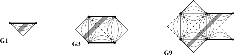
Figure 6.17: Cylinders from G1,3,9. The opposite sides of the shaded strip have to be identified along the Killing lines (cf also Fig. 6.23). Note that in G3,9 there occur closed Killing horizons (broken lines), which leads to pathologies of the Taub–NUT type.

Next G3: Clearly also in this case we can identify $x^{1}$ with $x^{1}+\omega$ in a chart (5.5); obviously the resulting metric is completely smooth on the cylinder obtained, the fundamental region of which is drawn in Fig. 6.17. However, this cylinder has some pronounced deficiencies: Not only does it contain closed timelike curves as well as one closed null-line (the horizon); this spacetime, although smooth, is geodesically incomplete. There are, e.g., null-lines which wind around the cylinder infinitely often, asymptotically approaching the horizon while having only finite affine length (Taub–NUT spaces, see section 6.2.4.3). So, from a purely gravitational point of view such solutions would be excluded. Having the quantum theory in mind, one might want to regard also such solutions. Being perfectly smooth solutions on a cylinder, certainly they will be contained in the RPS of the Hamiltonian theory. We leave it to the reader to exclude such solutions by hand or not.

The above Taub–NUT solutions are not the only dubious ones. Take any maximally extended spacetime, remove a point from it, and consider the $n$-fold covering of this manifold: clearly the resulting spacetime is incomplete. However, for $n\neq 1$ it is impossible to extend this manifold so as to regain the original spacetime. This is a very trivial example of how to obtain an in some sense maximally extended $2n$-kink solution from any spacetime. In the presence of a Killing vector there are, however, more intricate possibilities of constructing kinky spacetimes (resulting, e.g., also in inextendible 2-kink solutions, even flat ones); we postpone their discussion to section 6.2.5. These solutions are certainly not global in the sense pointed out before. Excluding them as well as the Taub–NUT type spaces from G3, the above solutions are all global solutions for the KV–model with negative cosmological constant $\Lambda$. In particular we see that the topology of spacetime is planar or cylindrical only. Also the RPS ($\Sigma=S^{1}$) is found to have a simple structure: It is a plane, parameterized by $C$ and $\omega$.

Now the KV–model with $\Lambda>0$: The discussion of G1,3 is as above. Also for G9,11 an identification $x^{1}\sim x^{1}+\omega$ in a chart (5.5) leads to a smooth (but incomplete) cylinder again. However, for G9,11 there are also cylindrical solutions without any deficiencies. Take, e.g., G9: Instead of extending the patch from Fig. 6.16 infinitely by adding further copies one could take only a finite number of them and glue the faces on the left and the right side together (cf Fig. 6.18). Clearly the result will be an everywhere smooth, inextendible spacetime. Also it permits a global foliation into $\Sigma\times{R}$ with a spacelike $\Sigma\sim S^{1}$. Now, however, the ‘size’ of the closed universe is ‘quantized’ (the circumference being fully determined by the (integer) number of blocks involved). Still, there is some further ambiguity in the gluing process that leads to a one-parameter family of diffeomorphism inequivalent cylinders for any fixed value of $C$ and fixed block number. This second quantity, conjugate to $C$ in a Hamiltonian formulation, and its geometric interpretation shall be provided in section 6.2.4 (cf Fig. 6.27) below.

Figure 6.18: Non–Taub–NUT cylinder from G9.

Thus in the case of G9 (and similarly of G11) we find the solution space for cylindrical spacetimes to be parameterized by $C$ (within the respective range, cf Fig. 6.13), by an additional real gluing parameter, and by a further discrete label (block number). For G9 there is also the possibility of solutions on a Möbius strip: We only have to twist the ends of the horizontal ribbon prior to the identification. It will be shown that these nonorientable solutions are determined uniquely already by fixing $C$ and the block number; there is now no ambiguity in the gluing!

By far more possibilities arise for G11. Again there are cylinders of the above kind, with an analogous parameterization of these solutions. However, now we can also identify faces in vertical direction (cf Fig. 6.16). For instance, gluing together the upper and lower ends as well as the right and left ends of the displayed region, one obtains a global solution with the topology of a torus with hole. (It has closed timelike curves (CTCs), but no further defects; also there are tori without CTCs.) The solution space for this topology is three-dimensional now, the two continuous parameters besides $C$ resulting from inequivalent gluings again. In addition, G11 permits much more complicated global solutions. In fact, it is one of the examples for which solutions on all (reasonable) noncompact topologies exist. Fig. 6.19 displays two further examples: A torus with three holes and a genus two surface with one hole. The respective fundamental regions (for the topologically similar solution R5) are displayed in Fig. 6.30 below. As a general fact the dimension of the solution space exceeds the rank of the respective fundamental group by one, and thus it coincides with twice the genus plus the number of holes. Also, there occur further discrete labels.

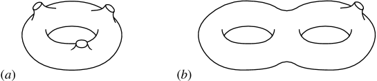
Figure 6.19: Factor spaces from G11. The corresponding fundamental regions are similar to those given in Fig. 6.30 for R5.

6.2.2.1 The moduli space for $M\sim\Sigma\times\mbox{{\sl I R}}$

In conclusion, let us consider the RPS (= the solution space for topology $S^{1}\times R$) in the case of $\Lambda>1$ (simultaneous existence of G9 and G11, cf Fig. 6.13). It is two-dimensional, being parameterized locally by $C$ and the respective conjugate ‘gluing’ variable. However, for $C$ taken from the open interval $]C_{-},C_{+}[$ (where $C_{\pm}(\Lambda)=-4\left(\pm\sqrt{\Lambda}-1\right)\exp\left(\pm\sqrt{\Lambda}\right)$, cf Fig. 6.13 and equation (6.21)) there are infinitely many such two-dimensional parts of the RPS, labelled by their ‘block number’. More precisely, for sufficiently large negative numbers of the (canonical) variable $C$ ($C<C_{-}$) the RPS consists of one two-dimensional sheet. At $C=C_{-}$ this sheet splits into infinitely many two-dimensional sheets. At $C=0$, furthermore, any of these sheets splits again into infinitely many, all of which are reunified finally into just one sheet for $C\geq C_{+}$. Furthermore, at $C_{\pm}$ and $0$ the RPS is nonHausdorff.

So, while for $\Lambda<0$, where the RPS was found to be planar globally, a RPS quantization is straightforward, yielding wavefunctions $\Psi(C)$ with the standard inner product (cf 7 for further details), an RPS quantization is not even well-defined for $\Lambda>0$ (due to the topological deficiencies of the RPS). In a Dirac approach to quantization (cf also 7 below), on the other hand, related problems are encountered when coming to the issue of an inner product between the physical wave functionals: For $\Lambda>1$, e.g., the states are found to depend on $C$, again, but for $C\in\;]C_{-},0[\,$ there is one further discrete label, and for $C\in\;]0,C_{+}[\,$ there are even further labels. When no discrete indices occur, as is the case for $\Lambda<0$, an inner product may be defined by requiring that the Dirac observable $\omega$ conjugate to $C$ becomes a hermitian operator when acting on physical states [129]; this again leads to the Lebesgue measure $dC$ then (cf also section 7.2.2.3). Such a simple strategy seems to fail for $\Lambda>0$ (and also any generic case of (3.15)!).

Certainly one could require that only cylinders of the kind Fig. 6.17 (states with block number ‘zero’) contribute to the inner product. However, at least in view of the corresponding classical solutions, this seems hardly satisfactory: For G9, e.g., i.e. for $C\in\,]C_{-},0[$, we found precisely the above solutions to be somewhat pathological, while those of nonzero block number (Fig. 6.18) were perfectly admissible!

This is thus found as one of the points where an improvement of quantization schemes may set in.

6.2.3 A global $\sigma$-model approach

In section 5.1.2 we determined the (local) solutions to the field equations of the Poisson $\sigma$-models describing 2d gravity theories by using Casimir-Darboux (CD) adapted field variables. As CD coordinates exist locally on the target space $N$ only, we cannot just apply the procedure directly in the global context without adapting it appropriately.

In this section we will provide a classification of the global solution for the pure gravity models. As remarked already in section 6.2.1, the classification within (the present status of) this approach will provide only an upper bound to the dimension of the moduli space. The additional requirement for globally nondegenerate metrics is not yet taken care of. It should be possible, however, to improve on this.

Pure 2d gravity models are described by means of a PSM with target space $N=\mbox{{\sl I R}}^{3}$ and Poisson tensor (4.8). The symplectic leaves are either two- or zero-dimensional.

We first focus on the map ${\cal X}$ from the spacetime (worldsheet) $M$ into the target space $N$. In the neighborhood of any (generic) point we may introduce CD coordinates. In such coordinates, the field equations yield $dC=0$. From this we may follow, that the image of ${\cal X}$ has to lie entirely within a symplectic leaf. This is already a global result, obtained by patching together different charts with CD coordinates. (As may be shown, it also holds for ‘nongeneric’ points in $N$, i.e. for zero dimensional leaves.)

Moreover, as becomes obvious upon inspection of the symmetries (4.14), any smooth deformation of the map ${\cal X}$ is a gauge symmetry. If ${\cal X}$ is contractable, in particular, a gauge representative may be chosen, such that $M$ is mapped into a single point only. For a generic leaf this corresponds to a degenerate ($=$ noninvertible) metric (cf e.g. equation (5.24) or (5.39)). This is not so dramatic locally, however. Locally one always may use a gauge transformation such that the image of a small region in $M$ is two-dimensional and then a nondegenerate metric is available. Providing merely an upper bound to the dimension of the moduli space, we do not need to check, if globally a nondegenerate metric can be obtained by means of the PSM symmetries out of a particular gauge representative. It is sufficient to determine the dimension of the solutions identified by means of PSM symmetries. (Recall that these symmetries coincide with the gravitational symmetries for nondegenerate metrics. They are only somewhat stronger, as they allow to gauge transform a nondegenerate metric into a degenerate one. The very same mechanism works also in 2+1 gravity [130]. We will further discuss this issue in chapter 7.

In general there will, however, be maps ${\cal X}$ also, with an image that may not be contracted to a point. We thus obtain a discrete label for the classical solutions, which characterize the homotopy classes of maps $M\to N$. These labels are in one-to-one correspondence with the block number(s) mentioned in the other two approaches within the present chapter (or the conjugacy classes of the discrete groups).

This completes the discussion of the fields $X^{i}(x)$. The more difficult part is now the determination of gauge inequivalence classes of the fields $A_{i}$. More precisely, this part is nontrivial only, provided ${\cal X}$ is noncontractable (otherwise we can use CD again, inducing globally well-defined fields on $M$.)

For this purpose we return to the more abstract language, in which $A=A_{i}dX^{i}$ is regarded as a one-one-form on $M\times N$. Then we have

Theorem 1. Any $A_{i}\equiv{\cal X}^{*}(\partial_{i}\rfloor A)$ of the form

$$A_{i}={\cal X}^{*}(\partial_{i}\rfloor\bar{\Omega})$$ (6.22)

solves the field equations (4.16) and (4.17) (globally), provided only $\bar{\Omega}$ is a closed pseudo-inverse of ${\cal P}$.

In the above $\rfloor$ denotes the insertion of the respective vector field into the respectively subsequent differential form.

We know that ${\cal P}$ has no inverse, as it has a (generically one-dimensional) kernel. A pseudo-inverse $\bar{\Omega}$ is a matrix (two-form) coming as close to an inverse as possible: its defining property is $\bar{\Omega}{\cal P}\bar{\Omega}=\bar{\Omega}$. Clearly, the pullback of $\bar{\Omega}$ to a symplectic leaf is determined uniquely and equals the symplectic form $\Omega$ introduced already before. There certainly is some ambiguity in defining $\bar{\Omega}$; we will come back to this shortly.

Theorem 1 follows from noting that it is formulated in a target space covariant way and that, on the other hand, it is in agreement with (5.23) and (5.24) upon specialization to (local) CD coordinates. (A similar argumentation is often applied in general relativity after using Riemann normal coordinates to establish a result.) Note that within the theorem we may also replace $\partial_{i}$ by some arbitrary vector field $v$ on the target space.

More important in the present context, is, however, the following theorem:

Theorem 2. In the case that the orthonormal bundle of the symplectic leaf ${\cal S}\supset\mbox{Im}({\cal X})$ may be trivialized, the general local solution of $A$ is provided by

$$A_{v}:\equiv{\cal X}^{*}(v\rfloor A)={\cal X}^{*}(v\rfloor\bar{\Omega})+\alpha{\cal X}^{*}(v\rfloor dC)\,,$$ (6.23)

where $C$ is some Casimir function and $\bar{\Omega}$ a closed pseudo-inverse of ${\cal P}$ (both defined in a neighborhood of ${\cal S}$), and $\alpha$ is a closed one-form on $M$. The gauge inequivalence classes of $A$, moreover, are in one-to-one correspondence with elements of $\mbox{H}^{1}(M)$.

We will not provide the details of the proof here. Sufficiency is demonstrated along the same lines as for Theorem 1. For the converse direction of the proof, we used the fact that the orthonormal bundle of Im$({\cal X})$ (i.e., of the symplectic leaf under consideration) may be trivialized. This ensures that a vector field $\partial/\partial C$ nowhere parallel to Im$({\cal X})$ may be found. It may be possible to relax or even drop this assumption. (This is suggested, e.g., by the known correspondence of gauge-inequivalent solutions of YM gauge theories to elements of $\mbox{H}^{1}(M)$ for each independent Casimir element of the gauge group.)

Note also that the choice of the Casimir function $C$ is irrelevant in (6.23), as a change $C\to f(C)$ only rescales $\alpha$ by a constant.

Let us remark, moreover, that a change in the choice of $\bar{\Omega}$ produces a term like the second one in (6.23). So at least part of the freedom in choosing elements of the first cohomology of $M$ may be transferred also to the freedom of selecting a pseudo-inverse. (Possibly this permits a simplification of the statement.) However, within the present formulation of the theorem, $\bar{\Omega}$ is fixed (and any fixed choice will do).

It remains to note that in the case of pure 2d gravity, the (generic) symplectic leaves have codimension one and thus their orthonormal bundle is trivial always.

We now have achieved the classification we strived for:

Theorem 3. Any point in the moduli space of a PSM with bracket (4.8) is in one-to-one correspondence to a homotopy class of maps from $M$ into a symplectic leaf ${\cal S}$ and an element from $H^{1}(M)$. Thus, $\mbox{dim}({\mbox{moduli space}})=\mbox{dim}(\pi_{1}(M))+1$.

Here, by moduli space we mean all globally smooth solutions to the field equations modulo the PSM symmetries (4.14), (4.15)!

Since some of those solutions will not permit PSM gauge transformations such that the metric $g=2A_{+}A_{-}$ (symmetric tensor product) is nondegenerate everywhere on $M$, Theorem 3 provides an upper bound for the dimension of the gravitational moduli space only. (Furthermore, from the gravitational point of view, an additional discrete label has to be introduced when also permitting kinky spacetimes, cf sections 6.2.5 and 7.2.1.5 below.)

As the results of the detailed group theoretical approach, collected in section 6.2.1.3 above, prove, the existence of globally nondegenerate representatives within a given PSM equivalence class depends only on topological features of the respective symplectic leaf (encoded in the parameter $n$ of section 6.2.1.3) and the topology of the spacetime (worldsheet). It thus may be expected that there is also a simple direct approach taking care of global nondegeneracy of the metric within the PSM language.

We add some preliminary considerations in this direction. The nondegeneracy of the metric may be formulated in an elegant way in the PSM language under the following assumptions: For solutions of the form (6.22) with a spacetime $M$ that is a covering of (or that is covered by) Im$({\cal X})\subset{\cal S}$, the degenerate points of $g$ correspond to points on ${\cal S}$ where the kernel of $\bar{\Omega}$ (which necessarily points out of ${\cal S}$, certainly) lies in an $X^{3}\equiv\phi=const$ surface. Further work along these lines should be pursued.

6.2.4 Systematic group theoretical approach

6.2.4.1 Preliminaries

The method employed for finding the multiply connected solutions will be to factor the universal covering solutions by a properly acting transformation group. Let ${\cal G}:=\mbox{\it Sym}({\cal M})$ be the symmetry group of the manifold ${\cal M}$. For any subgroup ${\cal H}\leq{\cal G}$ we can construct the factor- (or orbit-)space ${\cal M}/{\cal H}$ which consists of the orbits ${\cal H}x$ ($x\in{\cal M}$) endowed with the quotient topology (e.g. [131]). To pass from this approach to a cut-and-paste description choose a fundamental region, i.e. a subset ${\cal F}\subseteq{\cal M}$ such that each orbit ${\cal H}x$ intersects ${\cal F}$ exactly once. The group action then dictates how the points of the boundary of ${\cal F}$ have to be glued together (cf Fig. 6.20).

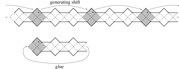
Figure 6.20: Cut-and-paste approach versus factorization. In the upper figure we indicated the action of a transformation group generated by a shift three copies to the right. To obtain the orbit space one identifies all sectors which are a multiple of three copies apart (e.g. all shaded patches). This space may be described equivalently by cutting out a fundamental region (lower figure) and gluing together the corresponding faces.

A priori orbit spaces may be topologically rather unpleasant, they need e.g. not even be Hausdorff. However, iff the action of this subgroup ${\cal H}$ is free and properly discontinuous, then the orbit space is again locally ${R}^{n}$ and Hausdorff, i.e. a manifold. If, furthermore, ${\cal H}$ preserves some (smooth, metric, etc.) structure or fields (e.g. $\Phi$), then the orbit space inherits such a structure in a unique way, i.e. the metric and the other fields are well-defined on ${\cal M}/{\cal H}$ (they ‘factor through’) and still fulfill the equations of motion (e.o.m.).

In this way one can obtain new ‘factor’-solutions of the e.o.m. We now want to sketch shortly that when starting in this way from the universal covering ${\cal M}$, one obtains all multiply connected global solutions: Given a multiply connected manifold $M$, one can always construct the (unique) simply connected universal covering space $\widetilde{M}$ and, furthermore, lift all the structure (metric, fields) to it. Certainly, the lifted fields again satisfy the e.o.m. (since these equations are purely local). Also, the lifted geodesics are geodesics on the covering space, and they have the same completeness properties. Thus the universal covering of a global solution is again a global solution of the e.o.m. and coincides with ${\cal M}$ (which was found to be determined uniquely, cf the previous chapter). Conversely, the original multiply connected solution $M$ can be recovered from the universal covering $\widetilde{M}={\cal M}$ by factoring out the group of deck-transformations. Let us note in passing that the fundamental group of a factor space is isomorphic to the group factored out, $\pi_{1}(M)\equiv\pi_{1}({\cal M}/{\cal H})\cong{\cal H}$ (more on this in [131]).

The solutions obtained by this approach are all smooth, maximally extended, and Hausdorff. Of course, if one is less demanding and admits e.g. boundaries (nonmaximal extension), conical singularities (failures of the differentiable structure), or violation of the Hausdorff-property, then there are many more solutions. We will shortly touch such possibilities in section 6.2.4.3 (Taub–NUT spaces) and section 6.2.5. On the other hand, from the point of view of classical general relativity even the globally smooth solutions may still have unpleasant properties such as closed timelike curves or the lack of global hyperbolicity (cf the previous section). In any case, our strategy will be to describe all of them; if necessary they may be thrown away afterwards by hand.

The metric (5.5) displays two symmetries, namely the Killing field $\partial\over\partial x^{1}$, generating the transformations

$$\widetilde{x}^{0}=x^{0}\quad,\qquad\widetilde{x}^{1}=x^{1}+\omega\,,$$ (6.24)

valid within one building block, and the (local) flip transformation provided by equation (6.2), valid within a sector, which has been used as gluing diffeomorphism for the maximal extension. The special family of nonnull extremals (6.13) provide possible symmetry axes for the flip-transformations (6.2) (cf dotted lines in Fig. 6.3).

The building block is usually incomplete (unless there is only one sector) and has thus to be extended. This process (described in detail in the previous chapter) consisted of taking at each sector the mirror image of the block and pasting the corresponding sectors together (using the gluing diffeomorphism (6.2)). Usually, overlapping sectors should not be identified, giving rise to a multi-layered structure, cf e.g. the spiral-staircase appearance of G4 (Fig. 6.24 below). Only where nondegenerate horizons meet in the manner of G3 (Figs. 6.16, 6.24, called bifurcate Killing horizons), the enclosed vertex point is an interior point (saddle-point for $\Phi$, called bifurcation point), and the overlapping sectors have to be glued together, yielding one sheet.

Any symmetry-transformation of a solution to the model (3.15) must of course preserve the function $\Phi$ (more generally, for the model (2.19) the functions $\phi$ and $X^{a}$) and also scalar curvature (and, if nontrivial, also torsion). However, by means of the e.o.m. of (3.15) the scalar curvature may be expressed in terms of $\Phi$ (cf also chapter 3). Similarly, for (2.19) curvature and torsion can by the e.o.m. be expressed in terms of the functions $\phi$ and $X^{a}$ (cf chapter 2). Moreover, since $X^{a}$ carries a Lorentz index, one only has to preserve $X^{2}\equiv X^{a}X_{a}$, which in turn may be expressed in terms of $\phi$ via another field equation (Casimir function $C\left[X^{2},X^{3}\right]=const$). Hence, in order to preserve all the functions above, it is sufficient to preserve $\phi$ only. (Recall that, in its specialization to vanishing torsion, ((2.19) describes (3.15) upon the identification $\Phi={\bf{U}}^{-1}(\phi)$; so $\Phi$ is preserved, iff $\phi$ is in this case (as common throughout the literature, ${\bf{U}}$ is assumed to be a diffeomorphism). Thus, also for notational simplicity, we shall speak of $\phi$ only; readers interested merely in (3.15) may, however, well replace ‘$\phi$’ by ‘$\Phi$’ in everything that follows.]

Finally, we shortly summarize some facts concerning free groups (details can be found in [131, 132]). A free group is a group generated by a number of elements $g_{i}$ among which there are no relations. The elements of the group are the words ${g_{i_{1}}}^{k_{1}}\ldots{g_{i_{l}}}^{k_{l}}$, subject to the relations (necessitated by the group axioms) $g_{i}{g_{i}}^{-1}=1$ and $g_{i}1=1g_{i}=g_{i}$ (the unit element 1 is the empty word). A word is called reduced, if these relations have been applied in order to shorten it wherever possible. Multiplication of group elements is performed simply by concatenating the corresponding words and reducing if necessary. While for a given free group there is no unique choice of the free generators, their number is fixed and is called the rank of the group. Free groups are not abelian, except for the one-generator group; if the commutation relations $ab=ba$ are added, then one speaks of a free abelian group.

Subgroups of free groups are again free. However, quite contrary to what is known from free abelian groups and vector spaces, the rank of a subgroup of a free group may be larger than that of the original group. The number of the cosets (elements of ${\cal G}/{\cal H}$) of a subgroup ${\cal H}\leq{\cal G}$ is called the index of ${\cal H}$ in ${\cal G}$. If this index is finite, then there is a formula for the rank of the subgroup $\cal H$:

$$\mbox{index $\cal H$}={\mbox{rank $\cal H$}-1\over\mbox{rank ${\cal G}$}-1}\,,$$ (6.25)

(cf [131, 132]). Especially, subgroups of finite index have never a smaller rank than the original group. On the other hand, $\mbox{rank $\cal H$}-1=n\cdot(\mbox{rank ${\cal G}$}-1)$ for some $n$ does not guarantee that the index of the subgroup $\cal H$ is finite; still, the question whether a given subgroup has finite index is decidable (cf [132]), but the algorithm is rather cumbersome.

6.2.4.2 The symmetry group

As pointed out above, any symmetry transformation must preserve the function $\phi$; thus sectors must be mapped as a whole onto corresponding ones (i.e. with the same range of $\phi$). Since $\phi(x^{0})$ is always monotonic (except for the deSitter solutions, which are therefore discussed separately in section 6.2.4.5), this has also the nice consequence that within one building-block a sector cannot be mapped onto another one. So each transformation gives rise to a certain permutation of the sectors and we can thus split it into (i) a sector–permutation and (ii) an isometry of a sector onto itself. Furthermore, it is evident that the whole transformation is already fully determined by the image of only one sector (the transformation can then be extended to the other sectors by applying the gluing diffeomorphism (6.2)).

Let us start with (ii), i.e. determine all isometries of one sector onto itself. Again $\phi$ must be preserved, so in the chart (5.5) the map must preserve the lines $\phi=const\Leftrightarrow x^{0}=const$. But also null-extremals must be mapped onto null-extremals. This leaves two possibilities: If the null-extremals (6.5) (i.e. $x^{1}=const$) are mapped onto themselves, then the only possibility is an overall shift of the $x^{1}$–coordinate, $x^{1}\to x^{1}+\omega$, i.e. a Killing-transformation (6.24). The gluing diffeomorphism (6.2) shows that such a transformation extends uniquely onto the whole universal covering, and that it is in all charts (5.5) represented as an $x^{1}$-shift of the same amount (but on the ‘flipped’ ones in the opposite direction!). In the neighbourhood of bifurcation points (simple zero of $h(x^{0})$) we can also use the local Kruskal-coordinates (6.17), where the same transformation reads $u\to u\exp(\frac{h^{\prime}(a)}{2}\omega)$, $v\to v\exp(-\frac{h^{\prime}(a)}{2}\omega)$, which looks in this case very much like a Lorentz-boost (cf e.g. the arrows around the bifurcation points in Figs. 6.27, 6.33 below). We will (thus) call these Killing-transformations shortly boosts and denote them by $b_{\omega}$. The composition law is clearly $b_{\omega}b_{\nu}=b_{\omega+\nu}$, so the boosts form a group isomorphic to I R, which shall henceforth be denoted by ${R}^{\rm(boost)}$.

If, on the other hand, the two families of null-extremals, (6.5) (i.e. $x^{1}=const$) and (6.6) (i.e. $dx^{1}/dx^{0}=-2/h$), are interchanged, then we obtain precisely the flip transformations. These transformations are the gluing diffeomorphisms (6.2), but this time considered as active transformations. Due to the constant in (6.2) the flips come as a one-parameter family; however, they differ only by a boost, i.e. given a fixed flip transformation $f$, any other flip $f^{\prime}$ can be obtained as $f^{\prime}=fb_{\omega}\equiv b_{-\omega}f\equiv{b_{\omega/2}}^{-1}fb_{\omega/2}$ for some $\omega$. We will thus consider only one flip and denote it by $f$. In the Carter-Penrose diagrams such a flip is essentially a reflexion at some axis (horizontal or vertical, according to sgn$\,h$; cf Fig. 6.21) and it is of course involutive (i.e. self-inverse, $f^{2}=1$). In the ‘Kruskal’-coordinates (6.17) it amounts essentially to an exchange $u\leftrightarrow\pm v$. Let us finally point out that while under a pure boost each sector is mapped onto itself (the corresponding sector–permutation is the identity), a flip transformation always (unless there is only one sector) entails a nontrivial sector–permutation (which is clearly self-inverse, since $f$ is).

We now turn to task (i), the description of the sector–permutations: As pointed out above, each transformation is fully determined by its action on only one sector. Let us thus choose such a ‘basis-sector’. If the transformation does not preserve orientation, we may apply a flip at this basis-sector and we are left with an orientation–preserving transformation. For these, however, the corresponding sector–permutation is already uniquely determined by the image of the basis-sector, i.e., for each copy of the basis-sector somewhere in the universal covering there is exactly one sector–permutation moving the basis-sector onto that copy. All these orientation–preserving sector–permutations thus make up a discrete combinatorial group (henceforth called $\{\hbox{sector-moves}\}$), which now shall be described in more detail.

Also choose a ‘basis-building-block’ and within this basis-block fix the first (or better: zeroth) sector as basis-sector (we label the sectors by $0,\ldots,n$ and the horizons between by $1,\ldots,n$). By a ‘basic move’ across sector $i$ we mean the following (cf Fig. 6.21): Go from the basis-sector to the $i$th sector of the basis-block and from there to the zeroth sector of the perpendicular (i.e. flipped) block. The corresponding sector-move, mapping the basis-sector onto this other sector, shall be denoted by $s_{i}$ (of course $s_{0}$ is the identity, $s_{0}=1$). Also the inverse basic moves can be easily described: One has to perform the same procedure at the flipped basis-block only (cf Fig. 6.21). An inverse basic move is thus the conjugate of the original move by a flip, $fs_{i}f={s_{i}}^{-1}$ (note $f=f^{-1}$). Here $f$ has been supposed to be a flip at the basis-sector. Flips at other sectors can be obtained by composition with sector-moves: $s_{i}f=f{s_{i}}^{-1}$ is a flip at sector $i$ of the basis-block (Fig. 6.21).

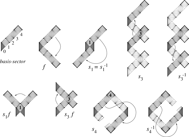
Figure 6.21: Some basic sector-moves, their inverses, and flips. The light shaded block is the basis-block resp. its image under the move, the dark shaded sector is the basis-sector (or its image). Only a few sectors of the universal covering are displayed. Note that the basic move $s_{4}$ and its inverse ${s_{4}}^{-1}$ transport the basis-block into different (but overlapping) layers of the universal covering. And note also that $s_{1}$, $s_{4}$, and their inverses turn the basis-block upside down!

Evidently there are two qualitatively different cases: If basis-sector and ‘flip’-sector are both stationary resp. spatially homogeneous, then the basic move is essentially a translation (e.g. $s_{3}$ in Fig. 6.21). However, if the sectors are of a different kind, then the move ($s_{1}$, $s_{2}$, $s_{4}$ in the example of Fig. 6.21) turns the whole solution upside down, inverting space and time (thus still preserving the orientation, as required for elements of $\{\hbox{sector-moves}\}$ — in contrast to, e.g., $s_{1}f$, which inverts space only, cf Fig. 6.21).

(Of course it is not necessary to choose the zeroth sector of the block as basis-sector. Let us denote the basic move across sector $i$ with basis-sector $k$ by $s_{i}\raisebox{5.59721pt}{\scriptsize$k$}$ (thus $s_{i}\raisebox{5.59721pt}{\scriptsize$0$}\equiv s_{i}$). They can, however, be expressed in terms of the old moves: As may be seen from Fig. 6.22 we have $s_{i}\raisebox{5.59721pt}{\scriptsize$k$}=s_{i}{s_{k}}^{-1}$, and consequently even $s_{i}\raisebox{5.59721pt}{\scriptsize$k$}=s_{i}\raisebox{5.59721pt}{\scriptsize$l$}\,\,\,\,s^{\smash{-}1}_{i}\raisebox{5.59721pt}{\scriptsize$l$}\hskip 9.47217pt$ for an arbitrary sector $l$. Obviously always $s_{k}\raisebox{5.59721pt}{\scriptsize$k$}\,\,=1$ (generalizing $s_{0}=1$) and $s_{i}\raisebox{5.59721pt}{\scriptsize$k$}=s^{\smash{-}1}_{k}\raisebox{5.59721pt}{\scriptsize$i$}\hskip 9.47217pt$. Thus, there is no loss of generality in choosing the basis-sector zero.)

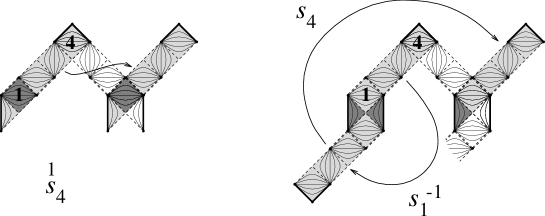
Figure 6.22: Basic sector-move with different basis-sector. As is seen from this figure the move $s_{4}\raisebox{5.03749pt}{\scriptsize$1$}$ can be composed of two moves with basis-sector zero, $s_{4}\raisebox{5.03749pt}{\scriptsize$1$}=s_{4}{s_{1}}^{-1}$. Although in this case ${s_{1}}^{-1}=s_{1}$ (relation at a bifurcation point), in general the right element has to be an inverse move!

The above basic moves $s_{i}$ form already a complete set of generators for $\{\hbox{sector-moves}\}$: By the extension process each location in the universal covering can be reached from the basis-sector by (repeated) application of the following step: Move through the basis-block or the flipped basis-block to some sector, then continue along the perpendicular block (i.e., applying a flip at this sector). But this step is exactly a basic move.

There may yet be relations between the generators. If, however, all horizons are degenerate, then there are no relations, and the resulting group is the free group with generators $s_{i}$. The reason is that in this case the vertex points between sectors are at an infinite distance (cf (6.14)) and thus the overlapping sectors (after surrounding such points) must not be identified, yielding a multilayered structure (cf e.g. $s_{4}$ in Fig. 6.21, or the ‘winding staircase’-like G4 in Fig. 6.24 below). A nontrivial word composed of basic moves $s_{i}$ describes such a move, which must therefore necessarily lead into a different ‘layer’ of the universal covering, since this manifold is simply connected.

The situation is different if there are nondegenerate horizons: In this case there are (interior!) bifurcation points at which four sectors meet, which then constitute a single sheet. Moving once around such a bifurcation point leads back to the original sector. Consequently there emerges a relation: If e.g. the first horizon is nondegenerate then the basic move $s_{1}$ turns the solution $180^{\circ}$ around with the bifurcation point as centre (cf Fig. 6.21). A second application of $s_{1}$ yields the original configuration again, so we have ${s_{1}}^{2}=1$. To find the analogous relations for a nondegenerate horizon say between the $(k-1)$th and $k$th sector it is wise to temporarily shift the basis-sector to the $k$th sector. Then evidently $s_{k-1}\raisebox{5.59721pt}{\scriptsize$k$}\hskip 12.05553pt$ turns the solution $180^{\circ}$ around that bifurcation point and we have the relation $(s_{k-1}\raisebox{5.59721pt}{\scriptsize$k$}\hskip 12.05553pt)^{2}=1$ which translates back to $(s_{k-1}{s_{k}}^{-1})^{2}=1$.

Summarizing, we have found that the group $\{\hbox{sector-moves}\}$ has the following presentation in terms of generators and relations ($n$ being the number of horizons):

$$\hbox{$\{\hbox{sector-moves}\}$}=\left\langle\;s_{1},\ldots,s_{n}\;\Big{|}\;(s_{k-1}{s_{k}}^{-1})^{2}=1\mbox{\ \ for each nondeg.\ horizon $k$}\;\right\rangle\,\,.$$ (6.26)

Any symmetry transformation can thus be written as a product of possibly a flip $f$ (if it is orientation-reversing), a sector-move from the group (6.26), and a boost $b_{\omega}$ ($\omega\in{R}$). Furthermore, this representation is unique, provided the elements are in this order. We have yet to describe the group product: Evidently boosts and sector-moves commute, since, as pointed out before, a boost is in all equally oriented charts (and sector-moves preserve the orientation) presented as a shift $x^{1}\rightarrow x^{1}+\omega$, equation (6.24). Furthermore, the conjugate of a boost by a flip is the inverse boost, $fb_{\omega}f=b_{-\omega}={b_{\omega}}^{-1}$, and the conjugate of a basic move by a flip is the inverse basic move, $fs_{i}f={s_{i}}^{-1}$, which also defines the conjugate of a general (composite) sector-move. The group product is thus completely determined, since in the formal product of two elements the factors can be interchanged to yield the above format. Thus the structure of the full isometry group is a semi-direct product

$${\cal G}=\hbox{${{{\bf{Z}}}_{2}}^{\rm(flip)}$}\ltimes\Big{(}\hbox{${R}^{\rm(boost)}$}\times\hbox{$\{\hbox{sector-moves}\}$}\Big{)},$$ (6.27)

where the right factor (in round brackets) is the normal subgroup, ${{{\bf{Z}}}_{2}}^{\rm(flip)}$ denotes the group $\{1,f\}$, and ${R}^{\rm(boost)}$ is the group of boosts described previously. Especially, if we restrict ourselves to orientable factor spaces and thus to orientation–preserving isometries, flips must be omitted and we are left with a direct product of the combinatorial group $\{\hbox{sector-moves}\}$ with ${R}^{\rm(boost)}$.

Still, this description is not always optimal, for two reasons: First, one is often interested in orientable and time–orientable solutions. Second, while for only degenerate horizons the group $\{\hbox{sector-moves}\}$ is a free group, this is not true if there are nondegenerate horizons (cf equation (6.26)). Interestingly, both problems can be dealt with simultaneously. Clearly the time–orientation–preserving sector-moves constitute a subgroup of $\{\hbox{sector-moves}\}$, which we shall denote by $\{\hbox{sector-moves}\}^{\uparrow}$ (in analogy to the notation used frequently for the orthochronous Lorentz group). If all horizons are degenerate and of even degree, then all sectors are equally ‘oriented’ (stationary or spatially homogeneous) and consequently all sector-moves are automatically time–orientation–preserving; thus $\hbox{$\{\hbox{sector-moves}\}^{\uparrow}$}=\hbox{$\{\hbox{sector-moves}\}$}$, and its rank equals the number of horizons.

This is no longer the case if there are horizons of odd degree. Then some sectors will have an orientation contrary to that of the basis-sector and a sector-move at such a sector will reverse the time–orientation (cf, e.g., $s_{1}$ in Fig. 6.21). The group $\{\hbox{sector-moves}\}^{\uparrow}$ is then a proper subgroup of $\{\hbox{sector-moves}\}$ (with index 2), which consists of all elements containing an even number of time–orientation reversing sector-moves.

Fortunately, this group can be described quite explicitly. Let us start with the case that there are nondegenerate horizons. To simplify notation we assume for the moment the first horizon to be nondegenerate (below we will drop this requirement). The sector-move $s_{1}$ is then an reflection at a bifurcation point and thus inverts the time–orientation (cf Fig. 6.21). But also the sector-moves around all other sectors ‘oriented’ contrary to the basis-sector (sectors 2 and 4 in Fig. 6.21) will reverse the time–orientation. The idea is to extract the space–time–inversion $s_{1}$ from the group $\{\hbox{sector-moves}\}$: For each sector $i$ introduce the new generators $s_{i}$ and $s_{1}s_{i}s_{1}$, if the $i$th sector has the same ‘orientation’ as the basis-sector, and $s_{i}s_{1}$ and $s_{1}s_{i}$, if it has the opposite ‘orientation’. These new generators are all time–orientation–preserving. Together with $s_{1}$ they obviously still span the whole group $\{\hbox{sector-moves}\}$ (relations between the new generators will be discussed presently). Conjugation by $s_{1}$ only permutes them among themselves (use ${s_{1}}^{2}=1$): $s_{i}s_{1}\leftrightarrow s_{1}s_{i}$ and $s_{i}\leftrightarrow s_{1}s_{i}s_{1}$. Also, any element of $\{\hbox{sector-moves}\}$ can be expressed as a word composed of the new generators with or without a leading $s_{1}$. Thus the group is a semidirect product

$$\hbox{$\{\hbox{sector-moves}\}$}=\hbox{${{{\bf{Z}}}_{2}}^{\rm(PT)}$}\ltimes\hbox{$\{\hbox{sector-moves}\}^{\uparrow}$},$$ (6.28)

where $\hbox{${{{\bf{Z}}}_{2}}^{\rm(PT)}$}=\left\{1,s_{1}\right\}\,$ (the ‘PT’ stands for parity and time–inversion) and $\{\hbox{sector-moves}\}^{\uparrow}$ is the group generated by the new elements given above (with $i\geq 2$). There may still be some relations among those generators: From (6.26) we know that any nondegenerate horizon $k$ adds a relation $(s_{k-1}{s_{k}}^{-1})^{2}=1$ or equivalently $s_{k-1}{s_{k}}^{-1}=s_{k}{s_{k-1}}^{-1}$. This yields a relation between the new generators, e.g. $(s_{1}s_{k-1}s_{1})(s_{k}s_{1})^{-1}=(s_{1}s_{k}){s_{k-1}}^{-1}$, by means of which either of the (four) generators involved can be expressed in terms of the remaining ones. Apart from those relations there are no further ones, so if we eliminate the redundant generators we are left with a free group! To determine the rank of this group note that each sector $>1$ contributes two generators and each nondegenerate horizon (except for the first, which was taken into account already in ${{{\bf{Z}}}_{2}}^{\rm(PT)}$) yields a relation which in turn kills one generator. Thus

rank $$\{\hbox{sector-moves}\}^{\uparrow} = 2\;(\mbox{number of degenerate horizons})+$$ (6.29)

$$\mbox{}+\mbox{number of nondegenerate horizons}-1\,\,.$$

Finally, if the first horizon is degenerate but the $k$th is not, then one can replace $s_{1}$ above by $s_{k-1}\raisebox{5.59721pt}{\scriptsize$k$}\hskip 12.05553pt$ and proceed in an analogous way. The result is (6.28), (6.29) again.

The remaining case to consider is the one in which all the horizons are degenerate. Then $\{\hbox{sector-moves}\}$ (6.26) is a free group and correspondingly its subgroup $\{\hbox{sector-moves}\}^{\uparrow}$ is free, too (cf section 6.2.4.1). Let us determine its rank: As noted already above, if all the horizons are of even degree, then $\hbox{$\{\hbox{sector-moves}\}^{\uparrow}$}\ =\hbox{$\{\hbox{sector-moves}\}$}$, and the rank equals the total number of (degenerate) horizons (thus (6.29) does not generalize to this case). Finally, assume that there is an odd-degree horizon and let it again be the first one (if it is not the first but the $k$th, just replace $s_{1}$ by $s_{k-1}\raisebox{5.59721pt}{\scriptsize$k$}\hskip 12.05553pt$ in what follows): A set of generators can be found in the same way as above (introducing $s_{1}s_{k}$, $s_{k}s_{1}$, or $s_{l}$, $s_{1}s_{l}s_{1}$, respectively, $k,l\geq 2$); however, now the element ${s_{1}}^{2}$, which no longer is the unit element, has to be added as a further generator. If $d$ denotes the number of (degenerate) horizons, we thus find $2d-1$ generators for $\{\hbox{sector-moves}\}^{\uparrow}$ (two for each degenerate horizon except for the first horizon, which adds one only). Here we also could have used formula (6.25), since $\{\hbox{sector-moves}\}^{\uparrow}$ has index 2 in $\{\hbox{sector-moves}\}$.

Let us finally summarize the above results:

Theorem: The group of space– and time–orientation–preserving symmetry transformations ${\cal G}_{+}^{\uparrow}$ is a direct product of I R with a free group,

$$\hbox{${\cal G}_{+}^{\uparrow}$}=\hbox{${R}^{\rm(boost)}$}\times\hbox{$\{\hbox{sector-moves}\}^{\uparrow}$}.$$ (6.30)

Let furthermore $n$ denote the number of nondegenerate horizons and $d$ the number of degenerate horizons. Then the rank of the free group $\{\hbox{sector-moves}\}^{\uparrow}$ is

$$d$$ if all horizons are of even degree,

$$2d+n-1$$ in all other cases. (6.31)

We will mainly work with this subgroup, but nevertheless discuss at a few examples how (time–)orientation-violating transformations can be taken into account.

6.2.4.3 Subgroups and factor spaces

We now come to the classification of all factor solutions. As pointed out in section 6.2.4.1, they are obtained by factoring out a freely and properly discontinuously acting (from now on called shorthand properly acting) symmetry group from the universal covering solutions. Thus we have first to find all properly acting subgroups of the full transformation group. However, not all different subgroups give rise to different (i.e. nonisometric) factor spaces. If, for instance, two subgroups $\cal H$ and ${\cal H}^{\prime}$ are conjugate (i.e., there is a symmetry transformation $h\in{\cal G}$ such that ${\cal H}^{\prime}=h{\cal H}h^{-1}$) then the factor spaces ${\cal M}/{\cal H}$ and ${\cal M}/{\cal H^{\prime}}$ are isometric. (Roughly speaking, this conjugation can be interpreted as a coordinate change). But also the converse is true:

Theorem:  Two factor spaces are isometric iff the corresponding subgroups are conjugate.

(for a proof cf e.g. [116], Lemma 2.5.6).
The possible factor spaces are thus in one-to-one correspondence with the conjugacy classes of properly acting subgroups. Still, apart from this abstract characterization it would be nice to have some ‘physical observable’, capable of discerning between the different factor spaces. This concerns mainly the boost-components of the subgroup elements, since information about the sector-moves is in a rather obvious way encoded in the global causal structure (number and arrangement of the sectors and singularities) of the factor space. Indeed we will in general be able to find such observables. [Here ‘physical observable’ means some quantity that remains unchanged under the group of diffeomorphisms (= gauge symmetry); so it will be a geometrical invariant, which not necessarily can be ‘measured’ also by a ‘physical observer’, strolling along his timelike worldline].

The above theorem is also valid for the case of a restricted symmetry group. For instance, a spacetime is often supposed to have — apart from its metric structure — also an orientation and/or a time–orientation. If the universal covering $\cal M$ carries a (time–)orientation and $\cal H$ is (time–)orientation–preserving, then also the factor space inherits a (time–)orientation. Now, if two subgroups are conjugate, ${\cal H}^{\prime}=h{\cal H}h^{-1}$, but the intertwining transformation $h$ does not preserve the (time–)orientation, then the corresponding factor spaces will have different (time–)orientations (while still being isometric, of course), and should thus be regarded as different. Thus, in this case the conjugacy classes of subgroups should be taken with respect to the restricted symmetry group (e.g. ${\cal G}_{+}^{\uparrow}$).

The requirement that the subgroup acts freely already rules out some transformations. First of all the subgroup must not contain pure flips at any sector: A flip has a whole line of fixed points, namely an extremal of the kind $dx^{1}/dx^{0}=-1/h$ (cf (6.13) and Fig. 6.3) as symmetry axis. This symmetry axis would become a boundary line of the factor space, which then would no longer be maximally extended. Consequently not only $f$, but also $f{s_{i}}^{n}$ and their conjugates have to be omitted.

But also reflections at a bifurcation point (turning the solution $180^{\circ}$ around this bifurcation point, e.g. $s_{1}$ in Fig. 6.21) must be avoided: Not only does the factor space fail to be time–orientable in this case, but also the bifurcation point is a fixed point, which upon factorization develops into a singular ‘conical tip’ making the solution nonsmooth. Thus, if the $k$th horizon is nondegenerate, then the elements $(s_{k-1}\raisebox{5.59721pt}{\scriptsize$k$}\hskip 12.05553pt)=s_{k-1}{s_{k}}^{-1}$ and conjugates thereof must not occur in the subgroup $\cal H$.

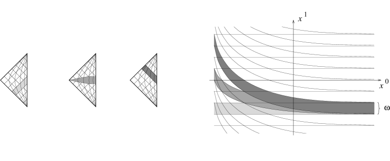
Figure 6.23: A cylinder resulting from pure boosts and possible fundamental regions $\cal F$; left in the Carter-Penrose diagrams, right in the EF-chart (5.5). Boundaries have to be glued along Killing-trajectories, i.e. along the curved lines in the left, resp. along vertical fibres in the right diagram.

Let us next assume pure boosts, which form a group isomorphic to I R (${R}^{\rm(boost)}$). The only discrete subgroups of boosts are the infinite cyclic groups generated by one boost, ${\cal H}_{\omega}:=\left\{{b_{\omega}}^{n},\,n\in{{\bf{Z}}}\right\},\>\omega>0$. In the coordinates (5.5) such a boost $b_{\omega}$ is a shift of length $\omega$ in $x^{1}$-direction. The factor space is then clearly a cylinder. Also, since boosts commute with sector-moves and ‘anticommute’ with flips ($fb_{\omega}=b_{-\omega}f$), the group ${\cal H}_{\omega}$ is invariant under conjugation and the parameter $\omega$ cannot be changed. Thus the cylinders are labelled by one positive real parameter $\omega$. In order to find some geometrical meaning of this parameter it is useful to adopt a cut-and-paste approach to the factorization procedure (used already intuitively in section 6.2.2): In the above example a fundamental region $\cal F$ can be obtained from the patch (5.5) by cutting out a strip of width $\omega$ parallel to the $x^{0}$-axis and gluing it together along the frontiers (preserving $x^{0}$, i.e. vertical fibres). Of course there are several choices for ${\cal F}$; it need not even be a horizontal strip, but any strip with vertical cross-section $\omega$ will work (cf Fig. 6.23). The width $\omega$ of this strip (i.e. of the generating shift) is proportional to the length of an $\phi=const$-path (resp. constant curvature or $\Phi$) running once around the cylinder. This is the desired geometrical observable: for any metric $g$ (i.e. function $h$ in (5.5)) we get a set of distinct solutions parameterized by their ‘size’ or circumference (any positive real number). Let us finally point out that this parameter $\omega$ has nothing to do with the Casimir-value $C$, present in the function $h$ of the metric. It is a new, additional parameter resulting from the factorization.

This all works perfectly well as long as there is only one sector, i.e., $h$ has no zeros, but at horizons the boosts do not act properly discontinuous. As a consequence the factor space will not be Hausdorff there. Furthermore, at bifurcation points the action is not free, so the factor space is not even locally homeomorphic to $\mbox{{\sl I R}}^{2}$ there. At the first glance this might seem surprising since when starting from an EF-coordinate patch (5.5) the construction of Fig. 6.23 should yield regular cylinders. They are not global, however: ‘half’ of the extremals approach the (closed) horizon asymptotically, winding around the cylinder infinitely often while having only finite length. This phenomenon is well-known from the Taub–NUT space or its two-dimensional analogue as described by Misner [133] (cf also [117]). A detailed description with illustrations can also be found in [134]. [In G3, Fig. 6.24, for instance, let the EF-coordinates cover the sectors I and II. The above class of incomplete extremals then comprises those which run across the lower horizon from I to IV, leaving the EF-patch. Thus to obtain an extension a second half-cylinder corresponding to IV has to be attached to I via a second copy of the closed horizon and likewise for the sector III, but of course this violates the Hausdorff property.] Similar results hold in general for solutions with zeros of $h(x^{0})$: whenever the group factored out contains a pure boost we obtain a Taub–NUT like solution (a cylinder-‘bundle’, where at each horizon, two sheets meet in a non–Hausdorff manner) labelled by its ‘size’ (metric-induced circumference along a closed $\phi=const$ line). If there are further sector–moves in the group $\cal H$, they have only the effect of identifying different sheets of this cylinder-bundle.

After these preliminaries we will now start a systematic classification of the factor solutions. We do this in order by number and type of horizons and illustrate it by the solutions of the JT–, $R^{2}$–, and KV–model (examples J1-3, R1-5, and G1-11, respectively; cf Figs. in the previous chapter, but also Figs. 6.16–6.18, 6.24–6.27).

No horizons (e.g. G1,2, J3):
This case has already been covered completely by the above discussion: There is only one sector, so $\{\hbox{sector-moves}\}$ is trivial. Furthermore, flips are not allowed, thus only boosts remain and they yield cylinders labelled by their circumference (positive real number).

In the following we will continue studying all factorizations possible for solutions with horizons. As pointed out before, there exist pathological Taub–NUT-like solutions for all of these cases (resulting from pure boosts). We will from now on exclude them, so pure boosts must not occur in the subgroup $\cal H$. But this also means that no sector–permutation can occur twice with different boost-parameters, since otherwise they could be combined to a nontrivial pure boost. This suggests the following strategy: factor out ${R}^{\rm(boost)}$ from $\cal G$, i.e. project the whole symmetry group onto ${\cal G}/\hbox{${R}^{\rm(boost)}$}=\hbox{${{{\bf{Z}}}_{2}}^{\rm(flip)}$}\ltimes\hbox{$\{\hbox{sector-moves}\}$}$, respectively ${\cal G}_{+}^{\uparrow}$ onto $\hbox{${\cal G}_{+}^{\uparrow}$}/\hbox{${R}^{\rm(boost)}$}=\hbox{$\{\hbox{sector-moves}\}^{\uparrow}$}$. All above (non–Taub–NUT) subgroups $\cal H$ are mapped one-to-one under this projection. One can thus ‘forget’ the boost-components, and first solve the combinatorial problem of finding the projected subgroups $\overline{\cal H}$ (which we will nevertheless simply denote by $\cal H$). Only afterwards we then deal with re-providing the sector-moves with their boost-parameters.

One horizon (e.g. G3-6, R1,2, J2): (Fig. 6.24)
The group $\{\hbox{sector-moves}\}$ is in these cases still rather simple: $\langle s_{1}|{s_{1}}^{2}=1\rangle\cong{{\bf{Z}}}_{2}$ for a nondeg. horizon (G3, R1), and $\langle s_{1}|-\rangle\cong{{\bf{Z}}}$ for the others. First of all we see that flips have to be omitted altogether: The most general form in which they can occur is $f{s_{1}}^{k}b_{\omega}$, but this is by the group product always conjugate to $f$ or $s_{1}f$ and thus a pure flip.

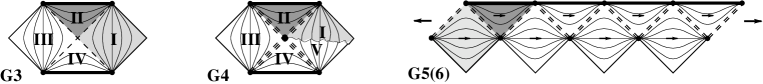
Figure 6.24: Carter-Penrose diagrams for one horizon (G3-6). For a nondegenerate horizon (G3) the vertex point is an (interior) bifurcation point and the manifold a single sheet. For degenerate horizons of odd degree (e.g. G4), on the other hand, this point is at an infinite distance, and thus the manifold has infinitely many layers. Finally, for horizons of even degree it is an infinite ribbon (G5(6), interior arrows indicate the Killing field).

The action of $\{\hbox{sector-moves}\}$ on the manifold is most evident for a zero of even degree, in which case we have the ribbon-structure of G5(6). Then $s_{1}$ is a shift of one block to the right (in the situation of Fig. 6.24). The nontrivial subgroups are the cyclic groups generated by ${s_{1}}^{n}$, for some $n\geq 1$, and the corresponding factor space is obtained by identifying blocks which are a multiple of $n$ blocks apart, i.e., gluing the $n$th block onto the zeroth. This yields a cylinder of a ‘circumference’ of $n$ blocks (see Fig. 6.25 for $n=3$). For degenerate horizons of odd degree (e.g. G4) the situation is rather similar, only the basic move is now a $180^{\circ}$-rotation around the (infinitely distant) central point, ‘screwing the surface up or down’ (i.e. mapping I $\rightarrow$ III, II $\rightarrow$ IV, III $\rightarrow$ V, etc.). Thus we get again cylinders of $n$ blocks circumference. When passing once around such a cylinder, however, the lightcone tilts upside down $n$ times, so we have got an $n$-kink-solution. Especially, the solutions with $n$ odd are not time–orientable. Finally, for nondeg. horizons (e.g. G3) the only nontrivial sector-move is $s_{1}$ (${s_{1}}^{2}$ is already the identity again), but this is the reflexion at the bifurcation point and thus not a free action. So we get no smooth factor solutions in this case.

If we had restricted ourselves a priori to orientable and time–orientable solutions, then we would have had to start from $\{\hbox{sector-moves}\}^{\uparrow}$. For G5(6) this makes no difference since then $\hbox{$\{\hbox{sector-moves}\}^{\uparrow}$}=\hbox{$\{\hbox{sector-moves}\}$}$, and indeed all cylinders were time–orientable in this case. For G4, on the other hand, $\{\hbox{sector-moves}\}^{\uparrow}$ is a proper subgroup, $\hbox{$\{\hbox{sector-moves}\}^{\uparrow}$}\cong 2{{\bf{Z}}}<{{\bf{Z}}}\cong\hbox{$\{\hbox{sector-moves}\}$}$, generated by ${s_{1}}^{2}$. This reflects the fact that only solutions of even kink-number are time–orientable. Finally, for G3 $\{\hbox{sector-moves}\}^{\uparrow}$ is trivial and there are no factor solutions at all.

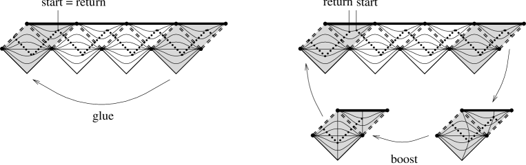
Figure 6.25: Boost-parameter for G5(6). In both cases the generating shift ${s_{1}}^{3}$ (or its inverse) is used to glue the right shaded patch onto the left one. If this generator has a nontrivial boost-component, then one has to apply a boost before gluing the patches (right figure). To illustrate the effect we have drawn a polygon of null-lines (pointed lines). Due to the boost the endpoint of this null-polygon will be shifted against the start, and this deviation may serve as a measure for the boost-parameter. Of course the same construction can also be applied to the other cases (e.g. G4, Fig. 6.24).

We have so far neglected the boost-component of the generator. After all the full-fledged generator of the subgroup will be ${s_{1}}^{n}b_{\omega}$! Does this have any consequences on the factor space? According to the theorem at the beginning of this section we must check whether the corresponding subgroups are conjugate. This is not the case here: The generator ${s_{1}}^{n}b_{\omega}$ of the subgroup commutes with everything except flips, and even a flip only transforms the group elements to their inverse, $f{s_{1}}^{n}b_{\omega}f={s_{1}}^{-n}b_{-\omega}=({s_{1}}^{n}b_{\omega})^{-1}$. Thus the group remains the same, and one cannot change the boost-parameter $\omega$ by conjugation. Let us again look for some geometrical meaning of this parameter. In the case of pure boosts discussed above (which also lead to cylinders) we have found the metric-induced circumference as such an observable. This cannot be transferred to the present case, however: there is no closed $\phi=const$-line along which a circumference could be measured, only the number of blocks $n$ ‘survives’. So we have to be more inventive: one could, e.g., take a series of null extremals, zigzagging around the cylinder between two fixed values of $\phi$ (see pointed lines in Fig. 6.21) and interpret the deviation from being closed, i.e. the distance between starting- and endpoint on this $\phi=const$-line, as measure for the boost. This distance is of course independent of the choice of the starting point on the $\phi=const$-line, but it depends on the two $\phi$-values; especially, these $\phi$-values can always be chosen such that the deviation is zero (closed polygon). This interpretation of the boost-parameter may be somewhat technical (we will find a much nicer one for e.g. G8,9 below), but there is certainly no doubt that the parameter is geometrically significant.

Two nondegenerate horizons (e.g. G8,9, J1):

Here $\hbox{$\{\hbox{sector-moves}\}$}=\langle s_{1},s_{2}\,|\,{s_{1}}^{2}=1,(s_{1}{s_{2}}^{-1})^{2}=1\rangle$, where the second relation may be replaced by $s_{1}s_{2}s_{1}={s_{2}}^{-1}$. With the help of these two relations any element can be expressed in the form ${s_{2}}^{n}$ or ${s_{2}}^{n}s_{1}$, and the group can thus (in coincidence with (6.28)) be written as a semi-direct product, $\hbox{${{{\bf{Z}}}_{2}}^{\rm(PT)}$}\ltimes{{\bf{Z}}}$, where $\hbox{${{{\bf{Z}}}_{2}}^{\rm(PT)}$}:=\{1,s_{1}\}$ and ${{\bf{Z}}}:=\{{s_{2}}^{n},n\in{{\bf{Z}}}\}=\hbox{$\{\hbox{sector-moves}\}^{\uparrow}$}$. However, not all those elements can be permitted: $s_{1}$ is a reflections at one bifurcation point, $s_{2}s_{1}=s_{2}\raisebox{5.59721pt}{\scriptsize$1$}$ is a reflection at the other bifurcation point, and the general element ${s_{2}}^{n}s_{1}$ is conjugate to one of them, thus also a bifurcation point reflection. The only freely acting group elements are thus the ${s_{2}}^{n}$ and they shift the manifold horizontally (in Figs. 6.26, 6.27) a number of copies side-wards. The factor space is then a cylinder. Each cylinder carries again a further real boost-parameter, but let us postpone this discussion and before admit flips (i.e. nonorientable solutions). The most general transformations involving flips (still omitting boosts) are ${s_{2}}^{n}f$ and ${s_{2}}^{n}s_{1}f$, but ${s_{2}}^{n}f$ and $s_{1}f$ are pure flips and cannot be used. A small calculation shows further that the only remaining admissible groups are those generated by one element ${s_{2}}^{n}s_{1}f$, $n\neq 0$. Since $s_{1}f$ is a flip at the middle sector (a reflection at the horizontal axis in Fig. 6.26) and ${s_{2}}^{n}$ a shift along that axis, the whole transformation is a glide-reflection and the factor space a Möbius-strip of $n$ copies circumference.

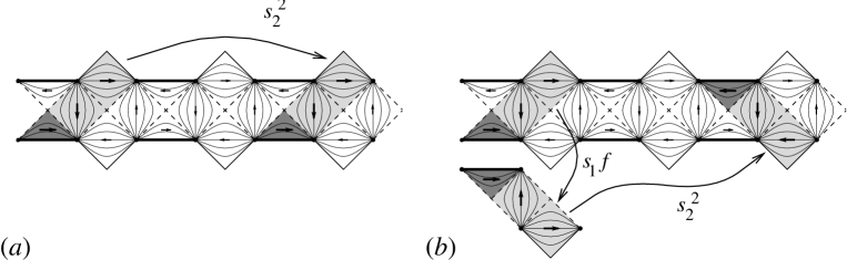
Figure 6.26: Sector-moves for G8,9; ${s_{2}}^{2}$ gives rise to a cylinder (a), while ${s_{2}}^{2}s_{1}f$ yields a Möbius-strip (b). Note that in (b) the (Killing-)arrows in the blocks identified by ${s_{2}}^{2}$ do not match.

Now concerning the boost-parameter: The complete cylinder-generator is ${s_{2}}^{n}b_{\omega}$. So we must check whether subgroups with different parameters $\omega$ are conjugate. Of course conjugation with $s_{2}$, $f$, and boosts does not change the parameter. However, conjugation with $s_{1}$ or $s_{1}f$ changes $\omega$ to its negative, $(s_{1}f)({s_{2}}^{n}b_{\omega})(s_{1}f)^{-1}={s_{2}}^{n}b_{-\omega}$. Hence the factor spaces corresponding to $\omega$ and $-\omega$ are isometric and one could consider to restrict the boost-parameter to nonnegative values, $\omega\in{{R}_{0}}^{+}$. However, the transformation $s_{1}f$ is a flip at the central sector, i.e., a reflection at the longitudinal axis (horizontal in Figs. 6.26, 6.27) and thus inverts the time. Hence, if the spacetime is supposed to have a time–orientation, then the generators with boost-parameter $\omega$ and $-\omega$ are no longer conjugate in the restricted symmetry group and the parameter has to range over all of I R.

In order to give this parameter a geometrical meaning we could of course employ the ‘zigzagging’ null-polygon again, but in this case there is a much nicer description: In Fig. 6.27 part of the infinitely extended solution G8,9 is drawn. A generating sector-move shifting the solution two copies (in this example) to the right dictates that the rightmost large patch (four sectors) is pasted onto the corresponding left patch. The boost-parameter then describes that before the pasting a boost has to be applied to the patch. As shown in Fig. 6.27 its effect is, e.g., that the thin timelike line crossing the right patch vertically has to be glued to the curved line of the left patch. The (shaded) region between these two lines is a possible fundamental region for this factor space! Also, due to the boost the spacelike tangent vector (arrow) to the dotted curve is tilted.

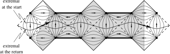
Figure 6.27: Fundamental region (shaded) and interpretation of the boost-parameter for G8,9. The right straight boundary has to be glued to the curved left one, and also the extremal (6.13) (dotted line) returns tilted (i.e. boosted).

In section 6.1 it was shown that the bifurcation points are conjugate points and the extremals running between them are those of (6.13) (in Fig. 6.27, they have been drawn as dotted lines). They run through the bifurcation points into all directions between the two null-directions. A boost bends them side-wards, altering the angle of their tangent. One can now start from a bifurcation point in a certain direction along a spacelike extremal. This extremal will eventually return to the original point, but due to a boost its tangent (cf arrow in Fig. 6.27) at the return may be tilted (boosted) against that at the start. This boost is of course independent of the chosen extremal and is thus a true ‘observable’; in particular, there is one solution without boost. Thus, the cylindrical solutions are parameterized by a positive integer (number of patches) and a real constant parameterizing the boost. As discussed before, if there is no time–orientation, then the boost-parameter has to be restricted to ${{R}_{0}}^{+}$. In the above interpretation of the boost-parameter this restriction arises if one cannot distinguish between boosts to the past or future. Of course, if a time–orientation is given, then such a distinction is possible. Note that in this case the (time–) direction of the boost is independent of the sense in which the extremal runs through the diagram.

It may seem that for the Möbius-strip one would also have such a continuous parameter due to different flips. However, this is not the case: Any two flips are conjugate (via a boost, $f^{\prime}\equiv fb_{\omega}=b_{-\omega/2}fb_{\omega/2}\sim f$), hence the corresponding subgroups are conjugate and all Möbius-strips are equivalent. (There is always one extremal (6.13) which returns unboosted). Also, in contrast to the former examples, a boost cannot be defined consistently on the Möbius-strip; the boost transformation does not ‘factor through’ the canonical projection onto the factor space. This is also seen immediately from Fig. 6.26 (b), where in the Möbius-case the sectors occasionally have to be identified with their mirror images and thus the arrows indicating the boost-direction do not match. However, locally this Killing symmetry is still present. Hence, the Möbius-strip solution is only parameterized by a positive integer (number of copies).

6.2.4.4 More than one generator

So far we have treated the cases where $\hbox{$\{\hbox{sector-moves}\}^{\uparrow}$}\cong{{\bf{Z}}}$ (one generator) or trivial. In those cases also all subgroups have been one-generator groups ${\bf{Z}}$, and the possible topologies have thus been restricted to cylinders and Möbius strips (remember that the subgroup $\cal H$ factored out equals the fundamental group of the factor space, $\pi_{1}({\cal M}/{\cal H})$). This situation changes drastically when there is more than one generator, as there are then subgroups of arbitrarily high rank (even infinite).

Ultimately we want to know the conjugacy classes of subgroups of $\{\hbox{sector-moves}\}^{\uparrow}$ (in this section we restrict ourselves to space– and time–orientable solutions; then all those subgroups are properly acting). Subgroups of free groups are again free, so in principle any solution can be obtained by the choice of a free set of generators. But this is only the easier part of the job:

• Given a subgroup (say, in terms of generators) it may be hard to find a free set generating this group.

• Also the free generators are by no means unique (one can, e.g., replace $g_{1}$, $g_{2}$, …by $g_{1}$, $g_{2}g_{1}$, …). Only the number of free generators (the rank of the subgroup) is fixed. So there is the problem to decide whether two sets of generators describe the same group or not.

• We have to combine the subgroups into conjugacy classes.

Since the group is free, these three issues can be solved explicitly (at least for finitely generated subgroups); however, the algorithms are rather cumbersome and thus we will not extend on this here (details in [132]).

Due to the more complicated fundamental groups it is to be expected that one gets interesting topologies. As already mentioned in section 6.2.1, all the solutions will be noncompact (this is also clear, since there is no compact manifold without boundary with a free fundamental group!). Thus it would be nice to have a classification of noncompact surfaces at hand. Unfortunately, however, there is no really satisfactory classification which could be used here (cf [131]). Let us shortly point out the wealth of different possibilities: A lot of noncompact surfaces can be obtained by cutting holes into compact ones. Of course the number of holes may be infinite, even uncountable (e.g. a Cantor set). A more involved example is that of surfaces of countably infinite genus (number of handles). Finally, there need not even be a countable basis of the topology (this does not happen here, though, since by construction there are only countably many building blocks involved). For an important subcase (finite index), however, the resulting topologies are always of the simple form ‘surface of finite genus with finitely many holes’.

Abstractly the index of a subgroup $\cal H$ is the number of cosets of $\cal H$. But it has also a nice geometrical meaning: Since $\{\hbox{sector-moves}\}$ acts freely and transitively on the sectors of the same type (and thus on the building blocks), the index of $\cal H$ in $\{\hbox{sector-moves}\}$ counts the number of building blocks in the fundamental region. Actually, since we started from $\{\hbox{sector-moves}\}^{\uparrow}$, it would be more convenient to use the index of $\cal H$ in that group. If all horizons are of even degree, then $\hbox{$\{\hbox{sector-moves}\}$}=\hbox{$\{\hbox{sector-moves}\}^{\uparrow}$}$ and there is thus no difference. On the other hand, if there are horizons of odd degree, then $\{\hbox{sector-moves}\}^{\uparrow}$ is a subgroup of index 2 of $\{\hbox{sector-moves}\}$ and consequently the number of building blocks is twice the index of $\cal H$ in $\{\hbox{sector-moves}\}^{\uparrow}$. This is also obvious geometrically, since the fundamental regions in this case are built from patches consisting of two building blocks (e.g. those situated around a saddle-point in the examples of Figs. 6.28 (b), 6.29 below). The index counts the number of these basic patches in the fundamental region then. For finite index, furthermore, it is correlated directly to the rank of $\cal H$ via formula (6.25) (with $\cal G$ replaced by $\{\hbox{sector-moves}\}^{\uparrow}$), thus

$$\mbox{index}\,{\cal H}=\mbox{number of basic patches}=\frac{\mbox{rank}\,{\cal H}-1}{n-1}\,$$ (6.32)

($n$ being the number of generators of $\{\hbox{sector-moves}\}^{\uparrow}$).

We will now provide the announced examples, starting with a discussion of the respective combinatorial part of the (orientation and time–orientation–preserving) symmetry group and followed by a discussion of possible factor spaces. Figures 6.28 and 6.29 contain basic patches as well as the generators of $\{\hbox{sector-moves}\}^{\uparrow}$. Although this group is the same in all these cases (rank 2), its action for R5 is different from the others, and correspondingly will be found to give rise to different factor solutions.

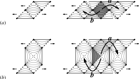
Figure 6.28: Basic patches and generators of $\{\hbox{sector-moves}\}^{\uparrow}$ for a fictitious example with two doubly degenerate horizons (a) and for R3 (b). Note that in the upper example the points in half height are at infinite distance, and that in the lower example the vertical singularities meet, yielding a slit (double lines). Going once around this point/slit leads into a different layer of the universal covering, as indicated by the jagged lines (multi-layered Carter-Penrose diagrams). Consequently $ab\neq 1$.

In the example Fig. 6.28 (a) (two doubly degenerate horizons) the group $\{\hbox{sector-moves}\}$ ($=\hbox{$\{\hbox{sector-moves}\}^{\uparrow}$}$) is free already, with the two generators $s_{1}$ and $s_{2}$. Geometrically, however, the moves with basis-sector 1 have a nicer representation. Let $a:=s_{2}\raisebox{5.59721pt}{\scriptsize$1$}\equiv s_{2}{s_{1}}^{-1}$ and $b:=s_{0}\raisebox{5.59721pt}{\scriptsize$1$}\equiv{s_{1}}^{-1}$. Clearly $a$ is a move one block to the right above the singularity and $b$ a move to the left below the singularity. Note that since we are in the universal covering their composition, $ab$, is not the identity but leads into another layer of the covering; if an identification shall be enforced, then the element $ab$ must occur in the subgroup factored out.

In Fig. 6.28 (b) only the second horizon is degenerate (G7,10, R3,4). Thus the basic patch consists of two building blocks. Here $\{\hbox{sector-moves}\}^{\uparrow}$ is a proper subgroup of $\{\hbox{sector-moves}\}$ and has the two free generators $s_{1}s_{2}$ and $s_{2}s_{1}$ (since the second sector is spatially homogeneous but the basis-sector stationary). Again, $a:=s_{2}s_{1}$ is a move one patch to the right above the singularity and $b:=s_{1}s_{2}$ a move to the left below the singularity. Thus the action is similar to that in Fig. 6.28 (a). However, if (time–)orientation–preservation is not required, then here one has the additional symmetries $f$ and $s_{1}$, i.e. reflection at the horizontal axis resp. at the saddle-point.

Our last example is R5, G11 (three nondegenerate horizons, cf Figs. 6.29, 6.16). Also in this case there are two free generators: $a:=s_{2}$, which is a move one patch upwards, and $b:=s_{3}s_{1}$, a move one patch to the right. (The other two potential generators can be expressed in terms of $a$ and $b$ by means of the saddle-point relations: $s_{1}s_{2}s_{1}=a^{-1}$ and $s_{1}s_{3}=a^{-1}b^{-1}a$). Again going once around the singularities leads into a new layer of the universal covering ($\Leftrightarrow[a,b]:=aba^{-1}b^{-1}\neq 1$).

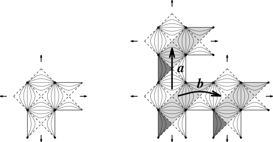
Figure 6.29: Possible basic patch and generators of $\{\hbox{sector-moves}\}^{\uparrow}$ for R5. As is seen here, the basic patch need not consist of two entire blocks, but the involved sectors may be rearranged somewhat.

Let us now determine the topology for the solutions with finite index. It is clear that then there are also only finitely many boundary segments. [This is a slightly informal terminology, since these ‘boundary segments’ (singularities, null infinities, points at an infinite distance) do not belong to the manifold. Still, this can be made precise and such boundaries are called ‘ideal boundaries’ or ‘ends’; we will thus simply use the notion boundary.] The generators of the subgroup $\cal H$ determine how the faces of the fundamental region have to be glued and thus also how the boundary segments are put together to form boundary components. This is shown at two examples in Fig. 6.30. There opposite faces should be glued together, which can be achieved by using the following generators: $b$, $a^{-1}ba$, $a^{-2}ba^{2}$, $a^{3}$ for the left case, and $b$, $a^{-1}b^{2}a$, $a^{-1}bab^{-1}a$, $a^{2}$ in the right case, provided one starts from the lowest basic patch. When starting from another patch, the subgroups and their generators will be conjugates of the above ones, but clearly this does not change the factor solution.

Now, topologically to each boundary component (which is clearly an $S^{1}$) a disk can be glued. This yields a compact orientable surface, which is completely determined by its genus. The original manifold is then simply this surface with as many holes as disks had been inserted (each boundary component represents a hole). The genus in turn depends on the rank of the fundamental group $\pi_{1}({\cal M}/{\cal H})\cong{\cal H}$ and on the number of holes:

$$\mbox{rank}\,{\cal H}=\mbox{rank}\,\,\pi_{1}({\cal M}/{\cal H})=2\,\,\mbox{genus}+\mbox{(number of holes)}-1\,.$$ (6.33)

Expressing the rank by means of (6.32), this yields

$$\mbox{genus}\,=\,\frac{(\mbox{number of basic patches})\cdot(n-1)-(\mbox{number of holes})}{2}+1\,,$$ (6.34)

where $n$ is the number of generators of $\{\hbox{sector-moves}\}^{\uparrow}$.

The general procedure to determine the topologies of the factor spaces can thus be summarized as follows: Draw a fundamental region for your chosen subgroup and determine which faces have to be glued together. Then count the connected boundary components (= number of holes) and calculate the genus from (6.34). We illustrate this procedure at two examples in Fig. 6.30.

Figure 6.30: Counting the boundary components (opposite faces have to be glued together). In both cases there are three basic patches (cf left part of Fig. 6.29) and thus (use (6.25) and $\mbox{rank}\,\hbox{$\{\hbox{sector-moves}\}^{\uparrow}$}=2$ !) four generators for $\cal H$, given in the text. However, due to the different number of boundary components (holes) the topologies differ, cf equation (6.34): In the left example there are three components ($a_{1,2}$, $b_{1,2}$, $c_{1\!-4}$), thus the topology is that of a torus with three holes. In the right example there is only one component ($a_{1\!-8}$); therefore this solution is a genus-2-surface with one hole. The resulting manifolds are shown in Fig. 6.19.

Some further examples for R5 are given in Fig. 6.31. Actually, they show that surfaces of any genus ($\geq 1$) and with any number ($\geq 1$) of holes can be obtained: continuing the series Fig. 6.31 (b), (c), (d) one can increase the number of handles arbitrarily, while attaching single patches from ‘below’ like in (e) allows one to add arbitrarily many holes.

Figure 6.31: Fundamental regions of factor spaces for R5. Opposite faces have to be glued together. (a) torus with six holes, (b) torus with one hole, (c) genus-2-surface with hole, (d) genus-3-surface with hole, (e) genus-2-surface with two holes.

For the cases of Fig. 6.28 (e.g. R3) the same analysis can be applied. For instance, it is obvious that cylinders with an arbitrary number of holes ($\geq 1$) can be obtained. Also surfaces of higher genus are possible; however, now the number of holes is always $\geq 3$ (past and future singularity, and at least one hole in ‘middle height’). [Note that this is no contradiction to the cylinder-with-hole case, since a cylinder with one hole is a sphere (genus-0-surface) with three holes]. In contrast to the R5-examples these factor solutions do not have closed timelike curves.

We turn to the cases with infinite index and thus infinite fundamental regions. All subgroups of infinite rank belong to this category, but also many subgroups of finite rank (see below). One topological reason for an infinite rank of the subgroup (and thus also of the fundamental group $\pi_{1}$) is the occurrence of infinitely many holes. For instance, it was pointed out that in the solution R3 (Fig. 6.28) the move $ab$ is not the identity but leads into a new layer of the universal covering. One can of course enforce the identification of overlapping layers by imposing the relation $ab\stackrel{{\scriptstyle!}}{{=}}1$ and its consequences. This is tantamount to factoring out the group generated by $ab$ and all its conjugates (the elements $a^{k}aba^{-k}$, $k\in{{\bf{Z}}}$, form already a free set of generators). The result is a ribbon with infinitely many holes (slits). Clearly the parameter space of such solutions is infinite dimensional now (cf also remarks at the end of this section). [If in addition one imposed the relation $a^{n}\stackrel{{\scriptstyle!}}{{=}}1$, then the previously infinite set of generators would boil down to $n+1$ generators ($a^{n}$, and $a^{k}aba^{-k}$ for $0\leq k<n$), and the resulting factor space (finite index again) would be a cylinder with $n$ holes.]

Likewise, in the example R5 (Fig. 6.29) the identification of overlapping layers is obtained by factoring out the infinitely generated commutator subgroup (generated freely e.g. by $a^{m}b^{n}ab^{-n}a^{-m-1}$, $(m,n)\neq(0,0)$; cf [131]); the factor space is a planar, double-periodic ‘carpet’ then. Adding, furthermore, the generator $a^{n}$ (or $b^{n}$) yields a cylinder with infinitely many holes (e.g. Fig. 6.31 (a) extended infinitely in vertical direction); and adding both $a^{n}$ and $b^{k}$ yields a torus with $nk$ holes, which is again of finite index.

Another possible reason for an infinite rank is an infinite genus (number of handles); such a solution is obtained for instance by continuing the series Fig. 6.31 (b), (c), (d) infinitely. Of course, both cases can occur simultaneously (infinite number of holes and infinite genus).

Let us now discuss the groups of finite rank and infinite index. Already the universal covering itself, being topologically an open disk (or $\mbox{{\sl I R}}^{2}$), provides such an example (with the trivial subgroup factored out). But also one-generator subgroups can by (6.25) never be of finite index (if $\mbox{rank}\hbox{$\{\hbox{sector-moves}\}^{\uparrow}$}\geq 2$). These subgroups yield proper (yet slightly pathological) cylinders without holes: Let ${\cal H}_{g}=\langle g\rangle\equiv\{g^{n},n\in{{\bf{Z}}}\}$ for arbitrary nontrivial $g\in\hbox{$\{\hbox{sector-moves}\}^{\uparrow}$}$. To speak in pictures: The generator $g$ of this infinitely cyclic subgroup defines a path in the universal covering. Now the end-sectors of the path (i.e. of the corresponding ribbon) are identified and at all other junctions the solution is extended infinitely without further identifications (cf Fig. 6.32). Thus a topological cylinder, although with a terribly frazzled boundary, is obtained (as before it is possible to smooth out the boundary by a homeomorphism). [The cylinders obtained in this way may have kinks of the lightcone or not. For instance, in the example Fig. 6.32 the lightcone tilts by (about) $90^{\circ}$ and then tilts back again. So, this is not a kink in the usual sense of the word; still, there is not one purely spacelike or purely timelike loop on such a cylinder.]

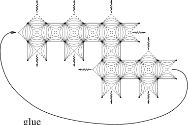
Figure 6.32: Frazzled cylinder from R5. Only the utmost left and right faces have to be glued together, such as to make a closed ‘ribbon’ of five patches (a possible generator for this gluing is e.g. $b^{2}a^{-1}b^{2}$). At all other faces (indicated $\rightsquigarrow$) the solution has to be extended without further identifications, similarly to the universal covering.

And even for higher ranks of $\cal H$ there are solutions of infinite index. The topologies obtained in this way are again of the simple form compact surface with hole(s). There is, however, a much greater flexibility in the rank (which is no longer restricted by formula (6.32)) as well as in the number of boundary-components (remember that in the examples Fig. 6.28 all solutions of finite index had at least three boundary-components). Indeed, one can obtain any genus and any nonzero number of holes in this way, as sketched in the following paragraph. Equation (6.33) is still valid, however, $\mbox{rank}\,{\cal H}$ can no longer be expressed by (6.32) but has to be determined directly from the gluings.

As already mentioned we may abuse the classification of compact two-manifold with boundary for our purpose; one has just to replace the true boundaries by ‘ideal boundaries’ which do not belong to the manifold. Note that the periphery of the basic patch consists of a couple of faces which have to be glued together pairwise, separated by (‘ideal’) boundary components. [It is topologically immaterial whether these boundary components are pointlike or extended singularities, since they do not belong to the manifold; each boundary point can be stretched to an extended segment by a homeomorphism and vice-versa.] The faces come in pairs and the number of pairs equals the rank of the group $\{\hbox{sector-moves}\}^{\uparrow}$. Thus in the present case there are at least two such pairs, which is sufficient to produce fundamental regions with arbitrarily many faces. Furthermore, by virtue of the infinitely branching extensions one can get rid of redundant faces: just extend the solution infinitely at this face so as to obtain a new (‘frazzled’) boundary segment which connects the two adjacent ones, yielding one larger boundary segment. Thus it is possible to produce polygons, the faces of which are to be glued in an arbitrary order. According to [131] this already suffices to produce all topologies announced above.

Finally, we have to discuss the boost-parameters. Since each free generator of $\cal H$ carries a boost-parameter, their total number equals the rank $r$ of this subgroup. Also an interpretation can be given in analogy to the cases dealt with before (zigzagging null-polygon and/or boosted saddle-point extremals). However, not all such choices of an $r$-tuple of real numbers are inequivalent. We show this at the example of the torus with three holes (Fig. 6.30, left part): There are four generators and thus also four boost-parameters, three of them describing the freedom in the horizontal gluing ($b$, $a^{-1}ba$, and $a^{-2}ba^{2}$) and one for the vertical gluing ($a^{3}$); let us denote them by $(\omega_{1},\omega_{2},\omega_{3};\omega_{4})$. Now, since conjugate subgroups lead to equivalent factor spaces, we can e.g. conjugate all generators with $a$. This leads to new generators, but since $a$ lies in the normalizer $\cal NH$ of $\cal H$ in $\{\hbox{sector-moves}\}^{\uparrow}$ they still span the same (projected) subgroup $\cal H$. Thus it is possible to express the old generators in terms of the new ones. However, during this procedure the boost-parameters change: For instance, the (full) first generator $\omega_{1}b$ is mapped to $a^{-1}\omega_{1}ba=\omega_{1}(a^{-1}ba)$, i.e. the parameter $\omega_{1}$ is shifted from the first to the second generator. Altogether, the three ‘horizontal’ boost-parameters $\omega_{1\!-3}$ are cyclically permuted and thus we get an equivalence relation among the 4-tuples, $(\omega_{1},\omega_{2},\omega_{3};\omega_{4})\sim(\omega_{3},\omega_{1},\omega_{2};\omega_{4})$. This is of course also geometrically evident: While the timelike loop corresponding to $\omega_{4}$ is uniquely characterized, the three spacelike loops corresponding to $\omega_{1\!-3}$ are indistinguishable (there is no ‘first one’).

In general, we have a (not necessarily effective) action of the group ${\cal NH}/{\cal H}$ on the space of boost-parameters ${R}^{r}$. Here $\cal NH$ is the normalizer of $\cal H$ in $\{\hbox{sector-moves}\}^{\uparrow}$ (or, if no (time–)orientation is present, also in $\{\hbox{sector-moves}\}$ or $\hbox{${{{\bf{Z}}}_{2}}^{\rm(flip)}$}\ltimes\hbox{$\{\hbox{sector-moves}\}$}$, respectively). The true parameter space is the factor space under this action, ${R}^{r}\big{/}({\cal NH}/{\cal H})$. Locally, it is still $r$-dimensional; however, since the action may have fixed points (e.g. in the above example the whole plane $(\omega,\omega,\omega;\omega_{4})$), it is an orbifold only.

6.2.4.5 Remarks on the Constant Curvature Case

So far we have only dealt with those solutions where the metric (or $\phi$–preservation) restricted us to only one Killing field. For reasons of completeness one should treat also the (anti-)deSitter solutions (5.54) of the general model, corresponding to the critical values $\phi={\phi}_{crit}$ and $X^{a}=0$, which have constant curvature (and zero torsion). Constant curvature manifolds have already occurred as solutions of the Jackiw-Teitelboim (JT) model [18], equation ((3.21), where, however, the symmetry group was still restricted to only one Killing field since $\phi$ had to be preserved. Here, on the other hand, these fields are constant all over the spacetime manifold, and thus the solutions have a much higher symmetry.

Already the flat case offers numerous possibilities: The symmetry group (1+1 dimensional Poincaré group) is generated by translations, boosts, and if space– and/or time–orientation need not be preserved, also by spatial and/or time inversion. As before pure reflexions would yield a boundary line (the reflexion axis) or a conical singularity (at the reflexion centre) and boosts a Taub–NUT space. The only fixed-point-free transformations are thus translations and glide-reflexions We have thus the following generators and corresponding factor spaces:

• One translation: Cylinders; parameters = length squared of the generating translation = circumference (squared) of the resulting cylinder (especially, there is only one cylinder with null-circumference).

• One glide-reflexion: Möbius-strips, again parameterized by their circumference.

• Two translations: Torus, labelled by three parameters: The lengths (squared) of the two generators $\vec{a}$ and $\vec{b}$ and their inner product. Globally, however, this is an overparameterization: Replacing, for instance, the translation vector $\vec{b}$ by $\vec{b}+n\vec{a}$ changes one length and the inner product, but still yields the same torus (just the original longitude is now twisted $n$ times around the torus).

• One translation and one glide-reflexion: Klein bottle. Here only two parameters survive (the inner product of the two generators can be conjugated away always). [This is somewhat similar to the situation cylinders versus Möbius strips in the case of G8,9 in section 6.2.4.3, where also a potential continuous parameter did not occur due to the nonorientability.]

Since two glide-reflexions combine to a point-reflexion or boost, and three translations generically yield a nondiscrete orbit, this exhausts all cases.

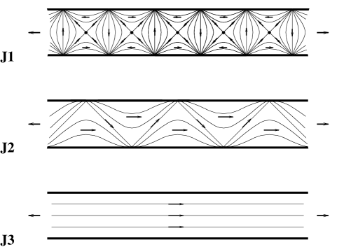
Figure 6.33: Killing fields for the JT–model and deSitter.

Now concerning the ‘proper’ ($R\neq 0$) (anti-)deSitter solutions resp. their universal coverings: Here the situation is slightly more involved. Of course all factor solutions of the JT–model (II,11) are also available for the (anti–)deSitter case, as both have constant curvature and zero torsion. For instance, the Killing fields corresponding to the solutions J1,2 give rise to cylinders labelled by block number and a boost-parameter, while J3 yields cylinders labelled by their (real number) circumference. Now, however, there are three independent Killing fields (e.g. J1,3 and their Lie-bracket) and thus one would expect further factor solutions. As an example, one has now in addition to cylinders also Möbius-strips of arbitrary circumference and not only of an integer number of blocks as in the case of J1 (G8,9). Unfortunately, the full isometry group of the space is $\widetilde{O}(2,1)$, whose connected component equals $\widetilde{SL}(2,R)$, and this group is famous for having no faithful matrix representation and is thus rather difficult to handle. A partial classification has been accomplished by Wolf [116], who deals with homogeneous spaces only and obtains a discrete series of cylinders and Möbius-strips for them. There are strong hints that even in the general case these are the only possible topologies (for instance, it would suffice to show that all properly acting subgroups of $\widetilde{SL}(2,R)$ are isomorphic to ${\bf{Z}}$.) However, a proof requires a different approach.

6.2.5 Remarks on kinks

The solutions obtained so far have all been geodesically complete, or, if not, the curvature or some physical field blew up at the boundary, rendering a further extension impossible. However, these global spacetimes are not all inextendible ones: it is, for instance, possible that the extremals are all incomplete, the fields and the curvature scalar remain all finite, yet when attempting to extend the solution one runs into problems, because the extension would no longer be smooth or Hausdorff or the like (cf e.g. the Taub–NUT cylinders of section 6.2.4.3). The purpose of this section shall be to give some further examples, to outline some general features of such solutions, and to discuss to which extent a classification is possible.

A familiar example for the above scenario is the metric [136]

$$g=e^{-2t}\left(-\cos 2x\,dt^{2}-2\sin 2x\,dt\,dx+\cos 2x\,dx^{2}\right)\,,$$ (6.35)

where the coordinate $x$ is supposed to be periodically wrapped up, $x\sim x+n\pi$. These are $n$-kink solutions, which means that, loosely speaking, the lightcone tilts upside-down $n$ times when going along a noncontractable nonselfintersecting loop on the cylindrical spacetime. For $n=2$, however, (6.35) is nothing but flat Minkowski space, the origin being removed, as is easily seen by introducing polar coordinates

$$\widetilde{x}=e^{-t}\cos x\,,\quad\widetilde{t}=e^{-t}\sin x$$ (6.36)

into the metric

$$g=d\widetilde{t}^{2}-d\widetilde{x}^{2}\,,$$ (6.37)

a fact that seems to have been missed in most of the literature. Consequently, the metric is incomplete at the origin; it has a hole which can easily be filled by inserting a point, leaving ordinary Minkowski space without any kink. For $n\neq 2$, on the other hand, (which are covering solutions of the above punctured Minkowski plane, perhaps factored by a point-reflection) this insertion can no longer be done, because it would yield a ‘branching point’ (conical singularity) at which the extension could not be smooth. Thus these manifolds are inextendible but nevertheless incomplete and certainly the curvature does not diverge anywhere ($R\equiv 0$).

Such a construction is of course possible for any spacetime, leading to inextendible $n\neq 2$-kinks. However, if there is a Killing symmetry present, then even in the 2-kink situation inextendible metrics can be obtained. To see this let us try to adapt the factorization approach of the previous section to these kink-solutions. First of all, since a point has been removed the manifold is no longer simply connected, so one must pass to its universal covering, which now winds around the removed point infinitely often in new layers (cf G3 versus G4 in Fig. 6.24). All above kink-solutions can then be obtained by factoring out a ‘rotation’ of a multiple of $2\pi$ (or $\pi$, if there is a point-reflection symmetry) around the hole. But according to the previous sections there should also occur a kind of boost-parameter. Is it meaningful in this context?

The answer to this question is yes, and this is perhaps best seen at the flat 2-kink example, the Killing field chosen to describe boosts around the (removed) origin. As long as the origin was supposed to belong to the manifold, smoothness singled out one specific boost value for the gluing of the overlapping sectors, leading to Minkowski space; otherwise there would have occurred a conical singularity at the origin. However, if this point is removed, then there is no longer any restriction on the boost-parameter. Its geometrical meaning is that after surrounding the origin a boost has to be applied before gluing or, in terms of fundamental regions, that a wedge has to be removed from the original (punctured) Minkowski space and the resulting edges are glued by the boost (also the tangents must be mapped with the tangential map of this boost, cf Fig. 6.34 a)). Of course, it is also possible to insert a wedge, but this is equivalent to removing a wedge from an adjacent (stationary) sector.

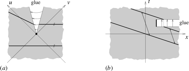
Figure 6.34: (a) Minkowski kink with nontrivial holonomy. This space can be obtained by removing a wedge from flat Minkowski space and gluing together the corresponding boundary lines by a boost. Due to this construction two extremals which are parallel on one side of the origin are mutually boosted on the other side (cf bold lines). Thus the holonomy is nontrivial (surrounding the origin yields a boosted frame), and at the origin there would occur a conical singularity. (b) Another inextendible Minkowski kink; it has trivial holonomy but the distance of parallels passing the hole changes.

Clearly such a space is everywhere flat (except at the origin, which is considered not to belong to the manifold) but has nontrivial holonomy. For instance, two timelike extremals which are parallel ‘before’ passing the origin at different sides will be mutually boosted afterwards (bold lines in Fig. 6.34 (a)).

In the above example we chose as Killing symmetry the boosts centered at the origin. However, Minkowski space also exhibits translation symmetries. An analogous construction can be applied also in this case with the following geometrical interpretation: cut out a whole slit (in direction of the chosen translation), remove the strip on one side of the slit, and glue together the resulting faces (cf Fig. 6.34 (b)). This manifold has now trivial holonomy, but the metric distance of two generic parallels passing the hole changes. Thus the manifold is so badly distorted that it cannot be completed to ordinary Minkowski space, either. In contrast to the former case this space can still be smoothly extended further: one can simply continue beyond the remaining left edge of the slit (bold line) into an overlapping layer whose upper and lower faces have to be glued together (since the endpoints of the slit have to be identified). This yields a maximally extended cylinder, where the (identified) endpoints of the slit constitute a conical singularity and should be removed.

It is relatively straightforward to write down the metric for the above examples in a circular region around the hole (but not too close to the hole), using smooth but nonanalytic functions. Analytic charts are more difficult to obtain, but at least for the case Fig. 6.34 (b) also this is possible (cf [137]). This last example, furthermore, can easily be generalized to an arbitrary metric with Killing symmetry: one has just to introduce Eddington-Finkelstein coordinates (5.5) in one patch. Then the analogous construction with $(x,t)\rightarrow(x^{0},x^{1})$ yields a one-parameter family of inextendible 2-kink solutions (resp. $2n$-kink). Explicit charts can be found in [137]. There is (sometimes) even the possibility to introduce discrete parameters like a ‘block-number’: one could, e.g., take G9 and make a long horizontal slit over a number of blocks, then remove a few blocks on the one side and glue together again (cf Fig. 6.35).

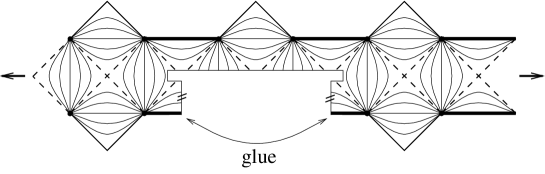
Figure 6.35: Yet another kink for G8,9.

It is somewhat problematic to give a complete classification of the kink solutions found above. Of course they could be described as factor spaces of limited coverings of the original universal covering solution. First, however, this would rather be a mere enumeration of the possible cases than a classification. Second, we do not want to distinguish two solutions, one of which is just an extension of the other. Thus we should only consider maximally extended limited coverings. In the above examples they all had only conical singularities, but it is not evident that this should be the most general scenario. Disregarding this question of the extension, the kinks are of course characterized by their kink-number, a (real) boost-parameter, and perhaps further discrete parameters (block-number or the like).

Finally we want to mention that such surgery is not restricted to cylindrical solutions (i.e. one hole only), but, within any of the global solution obtained in the previous sections, one can cut any number of holes, each giving rise to one boost-, one kink-, and perhaps some further discrete parameter. And as is well-known from complex analysis (Riemann surfaces), one can even obtain surfaces of higher genus (e.g. genus 1 with four branching points, etc.) in that way.

For further details on kinks we refer to [137]. This completes also our discussion of possible global solutions of the gravity models under discussion.

Chapter 7 Towards quantum gravity

The main part of this chapter is devoted to one particular quantization scheme applied to 2d gravity–YM theories, namely the so–called Dirac quantization [138]. The quantum treatment of theories with additional matter fields (and thus with propagating modes) is mentioned briefly only. In fact, even the Dirac quantization of the topological theories is not fully satisfactory yet, as, in the general case, the construction of an inner product between ‘physical quantum states’ is not available as of present day. We emphasize this because the purpose of lower dimensional models is to help us develop further current schemes of approaching the quantization of gravity theories.

Still, we will be able to find and classify all the physical states. The resulting space of states is found to crucially depend on the details of the potentials chosen in the original Lagrangian (cf equations (3.15) and (2.19)). Moreover, the classification of states will be seen to nicely fit to the classification of classical solutions for topology $\Sigma\times\mbox{{\sl I R}}$ as determined in the previous chapters.

Thus, there are some nontrivial results to be presented. However, even in the merely ‘topological’ case of pure 2d gravity-YM theories, there are still open problems on the technical as well as on the conceptual level, which we do not attempt to hide.

7.1 Hamiltonian formulation

According to chapter 4, the large variety of actions of gravity–Yang–Mills models can all be cast into the framework of Poisson $\sigma$-models (PSMs). In this section we will first provide the Hamiltonian structure of a general PSM (the increased generality poses no complication, rather notational simplicity is gained). Thereafter several issues of interest for quantization are addressed, like the construction of a reduced phase space (RPS). In the simplest cases, which includes, however, spherically symmetric vacuum Einstein gravity (SS) and string inspired dilaton gravity (SIDG) (cf sections 3.1.1 and 3.1.2), the RPS is just an $\mbox{{\sl I R}}^{2}$ and quantization is trivial. It is straightforward to extend the Hamiltonian formalism to also include, e.g., massless scalar fields. For this, however, we refer to the literature (cf., e.g., [53, 52]).

In general, a Hamiltonian formulation needs the restriction to spacetimes $M$ which, topologically, are of the form $M\sim\Sigma\times\mbox{{\sl I R}}$. For the case of a two–dimensional spacetime, $\Sigma$ can thus either be a circle or a line, only.

The former case is simpler and more transparent in two respects: First, as $\Sigma=S^{1}$ has no boundary, there is no room for boundary contributions to the Hamiltonian. The Hamiltonian framework can be made well–defined without bothering about (nontrivial) boundary conditions and contributions, which, in contrast, is necessary in the open case $\Sigma\sim\mbox{{\sl I R}}$ (where, again, one can distinguish between ‘bounded’ regions and infinitely extended ones).

Second, in the previous chapter, the moduli space, i.e. the space of classical solutions modulo gauge symmetries, was found to be of even dimension for cylindrical spacetime topologies, and of odd dimension for planar topologies. (E.g., in the case of pure SS this moduli space is one-dimensional, being parameterized by the Schwarzschild mass.) In the case of $\Sigma\sim S^{1}$, the RPS and the moduli space will be found to coincide, while for $\Sigma\sim\mbox{{\sl I R}}$ they are different. (To be precise, there are also two possible definitions of the moduli space on the Lagrangian level, depending on which precise notion of symmetries is used. Only for one of these choices, agreement with the RPS is obtained. We will come back to this below.)

We thus first start with the case of spacetimes of cylindrical topology and only then discuss the modifications necessary for the treatment of planar spacetimes.

7.1.1 For a cylindrical spacetime

The action of a PSM is already in first order form. It is therefore possible to compare it with a Hamiltonian action right away and read of Hamiltonians and constraints directly. For convenience of the reader we rewrite the action (4.12) or (4.13) here in component form, where, for the spacetime coordinates $(x^{0},x^{1})$, the more suggestive $(t,x)$ is used and, for notational simplicity, $A_{ri}:=A_{i}$, $A_{ti}:=\Lambda_{i}$, $\partial_{0}X^{i}\equiv\partial_{t}X^{i}:=\dot{X}^{i}$, and $\partial_{1}X^{i}\equiv\partial_{x}X^{i}:=\partial X^{i}$. (So within this section, $A_{i}$ does no more denote a one-form, but a function, or, better, $A_{i}\,dx$ a one–form on $\Sigma$, and, similarly, $x$ does no more denote a point on the two-manifold $M$, but just on $\Sigma$. We hope, this does not lead to any confusion.) Then (4.12) is rewritten identically as

$$L^{PSM}=-\int dt\oint_{S^{1}}dx\,[A_{i}\dot{X}^{i}-\Lambda_{i}(\partial X^{i}+{\cal P}^{ij}A_{j})]\,.$$ (7.1)

Our variables on phase space are $X^{i}(x)$ and $A_{j}(x)$, required to be $2\pi$-periodic $C^{\infty}$-functions of $x$. They are canonically conjugates; dropping the overall, and thus irrelevant, minus sign in front of (7.1), their field theoretic Poisson brackets are given by

$$\{X^{i}(x),A_{j}(y)\}=\delta^{i}_{j}\delta(x-y)\,,$$ (7.2)

while $\{X^{i}(x),X^{j}(y)\}=\{A_{i}(x),A_{j}(y)\}=0$. (The delta function on the right–hand side of (7.2) is understood as periodic delta function, certainly: $\sum_{n}\delta(x-y+2\pi n)$.) These Poisson brackets are sharply to be distinguished from the Poisson brackets generated by the tensor ${\cal P}$ on the finite-dimensional target space spanned by the coordinates $X^{i}$ (cf chapter 4):

$${\cal P}^{ij}=\{X^{i},X^{j}\}\,.$$ (7.3)

The variables $\Lambda_{i}$, on the other hand, are recognized as Lagrange multipliers for the constraints

$$G^{i}\equiv\partial X^{i}+{\cal P}^{ij}A_{j}\approx 0\,\,.$$ (7.4)

As suggested already by the notation, they are of first class. A straightforward calculation, making essential use of the Jacobi property of (7.3), yields

$$\{G^{i}(x),G^{j}(y)\}={\partial{\cal P}^{ij}\over\partial X^{k}}(X(x))\>G^{k}(x)\,\delta(x-y)\,.$$ (7.5)

Due to the diffeomorphism invariance of the underlying theory, the Hamiltonian is only a combination of the constraints: $H=-\oint_{0}^{2\pi}dx\Lambda_{i}G^{i}$. This comes as no surprise: After all, $H$ generates translations in $t$ and they are part of the local symmetries of the theory and thus should be generated by constraints. ‘On-shell’ then there is no nontrivial Hamiltonian in the theory, $H\approx 0$. In the context of the quantum theory (apparently there is no nontrivial Schrödinger equation) this gives rise to what is called the ‘problem of time’ in the literature (cf Introduction and section 7.2.2.3).

Let us note that up to now we did not require $t\equiv x^{0}$ to be timelike and $x\equiv x^{1}$ to be spacelike. The present formulation is flexible enough to describe also spacetimes $M$ of, e.g., the Taub-NUT type, where initially space-like circles $x^{0}=const$ turn into light- and timelike ones at later values of the evolution parameter $x^{0}$!

It is worthwhile to comment on the symmetries generated by the constraints, i.e., in more abstract terms, to study the flow of the Hamiltonian vector fields $\{\cdot,G^{i}(x)\}$, or, smearing out the distributional quantities by means of periodic test functions $\epsilon_{i}(x)$, the flow of the vector fields ${\cal V}_{\epsilon}:=\{\cdot,\oint\epsilon_{i}(x)G^{i}(x)dx\}$. By means of (7.2) and (7.4) we find:

$$\delta_{\epsilon}X^{i}(x)\equiv{\cal V}_{\epsilon}\,X^{i}(x) = \epsilon_{j}(x){\cal P}^{ji}(X(x))$$ (7.6)

$$\delta_{\epsilon}A_{i}\equiv{\cal V}_{\epsilon}\,A_{i}(x) = \partial\epsilon_{i}(x)+{\cal P}^{lm}{}_{,i}A_{l}\epsilon_{m}\,.\,.$$ (7.7)

These are just the spatial components of the PSM symmetries found in equations (4.14) and (4.15). Allowing $\epsilon$ to be also $t$–dependent, we thus may generate all the Lagrangian PSM symmetries (cf [139] for more details on the correspondence).

How are these symmetries related to the standard gravitational symmetries. Inspection of the Poisson tensor (4.8), characterizing the pure gravity models, shows that $G^{3}(x)$ generates the local Lorentz boosts in the frame bundle. $G^{\pm}(x)$, on the other hand, generate diffeomorphisms in null directions (up to Lorentz boosts). There are several ways of seeing this. The probably simplest one is the following [140]: By construction, the Hamiltonian $H$ is the generator corresponding to $\partial_{t}\equiv\partial_{0}$ on spacetime. $H\sim G^{+}$, on the other hand, implies $\Lambda_{-}\equiv A_{0-}=0$. However, $A_{0-}=e_{0}{}^{+}=0$ yields zero spacetime norm of $\partial_{0}$, which proves the assertion. (Eventual conformal rescalings of the metric, cf section 3.1.4.1, clearly do not affect this argument).

The symmetries generated by the $G^{i}$ thus contain the diffeomorphism symmetry and the local Lorentz symmetry present in the original formulation (provided Einstein–Cartan variables are used). As will be shown in a subsequent section, section 7.2.1.5, for invertible metrics also the converse holds: The diffeomorphisms and local Lorentz boosts contain the transformations generated by the constraints $G^{i}$; one thus establishes a bijection between the symmetries for such metrics. Since one usually restricts attention to invertible metrics, the difference of the flow of two kind of symmetries on degenerate metrics seems irrelevant. We will, however, have to come back to this issue in sections 7.2.1.4 and 7.2.1.5, when comparing the physical quantum states with the moduli space of the classical theory found in chapter 6.

One may also easily establish contact with lapse and shift. Recall, e.g., that $\Lambda_{i}\equiv A_{0i}$ and that the Hamiltonian vector field of $H=\oint A_{0i}G^{i}dx$ is the generator $\partial_{0}$ on spacetime. Thus, $\oint A_{1i}G^{i}dx$ corresponds to $\partial_{1}\equiv\partial_{x}$. So, the diffeomorphism constraint ${\cal H}_{x}$ is simply $A_{1i}G^{i}\equiv A_{i}\partial X^{i}$. As we will not need lapse and shift in what follows, we leave the rest as an exercise to the reader.

7.1.2 Modifications for open spacetimes

For $\Sigma\simeq S^{1}$, periodic boundary conditions for the variables in phase space are canonical, and there is no room for boundary terms in, e.g., the Hamiltonian since $\partial S^{1}=0$. A well–defined Hamiltonian formulation on $\Sigma\simeq\mbox{{\sl I R}}$, on the other hand, needs an additional external input. We are in the need to specify boundary conditions or asymptotic fall-off conditions and, simultaneously, have to take care for well–defined Hamiltonian vector fields [141] associated to functions on phase space which are of (physical) interest to us (such as the Hamiltonian $H$). The situation becomes technically involved easily and, in lack of uniqueness, sometimes nontransparent. In particular, we know from the classification obtained in section 6.1, that the moduli space of classical solutions on $M\simeq\mbox{{\sl I R}}^{2}$ modulo the gravitational (Lagrangian) symmetries is one-dimensional only. However, the reduced phase space (RPS) in a properly defined Hamiltonian framework necessarily is even-dimensional. Thus, during the process of selecting boundary conditions, somewhere a second moduli parameter will appear. We would like to see clearly, at which point this occurs (and, in a second step, what alternatives arise).

Again, also in the present context, the framework of $\sigma$-models will provide a well-adapted tool for transparency within this procedure. We focus on a Hamiltonian formulation on a bounded region $\Sigma$ (which, topologically, still is I R). An ‘infinitely extended’ $\Sigma$ may be visualized as a limit of the bounded case.

We will consider a region in spacetime bounded by two Killing lines. Denote the values of $\phi$ at these boundaries by $\phi_{R}$ and $\phi_{L}$, respectively. Fix the range of parameter $x$ to similarly lie between $x_{L}$ and $x_{R}>x_{L}$ (so the parameter is increasing from ‘left’ to ‘right’). Furthermore, fix the Lorentz frame at the boundary by requiring that $X^{+}$ equals 1 there. This is possible always, except if the boundary point coincides with a bifurcation point of the spacetime. (This exception does not bother us, if, at the end we are interested in the limiting case $x_{R,L}\to\pm\infty$, with similar conditions for $\phi_{L,R}$, depending, however, on the model considered. If, on the other hand, we want one of the boundaries to coincide with the bifurcation point (cf, e.g., [142]), we may require $X^{+}=X^{-}=0$ on that side of $\Sigma$, leaving $\phi$ unspecified there!) Summarizing, we require:

$$\phi(x_{L,R})\stackrel{{\scriptstyle!}}{{=}}\phi_{L,R}=const\;\;,\quad X^{+}(x_{L,R})\stackrel{{\scriptstyle!}}{{=}}1\;.$$ (7.8)

To determine eventual boundary contributions to the Hamiltonian $H$, we need to investigate the action functional (7.1) with the integral over $S^{1}$ replaced by an integral over $\Sigma$. We need to check, if the Hamiltonian, as read off from this action, has a well–defined Hamiltonian vector field (on the field theoretic phase space) [141]. The potentially troublesome terms are those with spatial derivatives acting on the canonical variables. Variation of (7.1) (with $S^{1}$ replaced by $\Sigma$) with respect to $X^{+}$ and $X^{3}$ leads to boundary contributions that vanish on behalf of (7.8). However, without further manipulations, this does not apply also to $\delta X^{-}$.

We now have two options: First, we may also require $X^{-}$ to be fixed at the boundary. Then, $H$ is functionally differentiable and the Hamiltonian formulation is well–defined. On the other hand we observe that when fixing $X^{-}$ beside $X^{+}$ and $X^{3}$ at the boundary, the boundary conditions also determine the symplectic leaf and the respective value of the Casimir $C$. As $C$ was the only local, gauge–invariant parameter left in the analysis on the Lagrangian level, it is plausible (and indeed the case) that such boundary conditions will lead to a zero–dimensional RPS. This is not very interesting, certainly. However, the RPS then is seen to be even–dimensional, as it should be, and this is also understood from the Lagrangian point of view: Fixing $C$ leaves only a single gauge–inequivalence class of classical solutions.

Our second option is to introduce a boundary term to the Hamiltonian action, the variation of which will cancel the undesired contribution. This is of the form $(\Lambda_{-}X^{-})_{R}-(\Lambda_{-}X^{-})_{L}$, where the suffix denotes evaluation at the respective boundary. It may appear that now we have shifted the problem to the variation of $\Lambda_{-}$ only (as the addition of the above boundary term amounts to a partial integration in the action, with the roles of $\Lambda_{-}$ and $X^{-}$ interchanged). However, $\Lambda_{-}$ is not a variable on phase space.

Next, we need to properly define the constraints. Here one usually requires the appropriate test functions $\varepsilon_{i}$ to become zero at the boundaries. Therefore the constraints are

$$\int_{\Sigma}\varepsilon_{i}(x)G^{i}(X(x))\,dx\approx 0\,\,\quad\mbox{with}\;\;\varepsilon_{i}(x_{L,R})=0\,.$$ (7.9)

(Note the target space covariance of the expression.)

To make sure that the boundary conditions (7.8) are conserved with respect to the flow of the Hamiltonian, we need to require that some combinations of the $\Lambda_{i}$ have to vanish at the boundary. These restrictions are deteremined most easily by using CD coordinates. Note that in the neighborhood of each of the boundary lines we may introduce CD coordinates $\widetilde{X}^{i}=({1\over 2}C,ln|X^{+}|,\phi)$, cf equation (5.37). In these coordinates, the boundary conditions (7.8) read: $\widetilde{X}^{2}(x_{L,R})=0$ and $\widetilde{X}^{3}(x_{L,R})=\phi_{L,R}$. The constraint densities $G^{i}(x)$ take the simple form:

$$\widetilde{G}^{1}=\partial{\widetilde{X}}^{1}\;,\quad\widetilde{G}^{2}=\partial{\widetilde{X}}^{2}+A_{\widetilde{3}}\;,\quad\widetilde{G}^{3}=\partial{\widetilde{X}}^{3}-A_{\widetilde{2}}\;.$$ (7.10)

Here and in what follows $A_{\widetilde{i}}\equiv\widetilde{A}_{i}$, $\widetilde{G}^{i}\equiv G^{\widetilde{i}}=(\partial\widetilde{X}^{i}/\partial X^{j})G^{j}$ etc. Thus, it is obvious that our boundary condtions are preserved, iff $\Lambda_{\widetilde{2}}$ and $\Lambda_{\widetilde{3}}$ vanish at the boundary. (These requirements are in no contradiction with $\det g\neq 0$, as one easily may verify.)

Since the fields $X^{i}(x)$ are required to be smooth (in $x$), we may follow from (7.9) that the value of the Hamiltonian $H$ is nonzero now:

$$H\approx(\Lambda_{-}{X}^{-})_{R}-(\Lambda_{-}{X}^{-})_{L}\,.$$ (7.11)

Note that due to (7.8), the value of $X^{-}$ at the boundary is a unique function of the Casimir $C$ at the boundary. In particular in the torsion–free theories $2X^{-}=C+const$ at the boundary (cf equation (4.9)). Then upon appropriate conditions on $\Lambda_{-}(x_{L,R})$ (or $\Lambda_{\widetilde{1}}(x_{L,R})$) the (value of the) Hamiltonian is found to coincide with the Casimir $C$. As shown in [104], up to an appropriate normalization constant, this quantity may be identified with the ADM mass, furthermore.

Now, with these definitions, the RPS will turn out to be two-dimensional (cf below for a simple proof). For the case of Schwarzschild (SS), this coincides with the result found in [143, 144].

Let us now shed some light on the appearance of the second parameter by comparing explicitly the Hamiltonian with the Lagrangian symmetries. By means of considerations completely analogous to the case $\Sigma\simeq S^{1}$, one may establish equivalence of the Lagrangian and the Hamiltonian symmetries inside of the region under consideration. However, in (7.9) the test functions were required to vanish at the boundary. Thus there the symmetries are frozen. So, there are less (gauge) symmetries available at the boundary in the Hamiltonian formulation as compared to the Lagrangian one.

On the other hand, we, however, also imposed boundary conditions, not present when determining the moduli space on the Lagrangian level. From the Lagrangian point of view, the boundary conditions (7.8) may be recognized as gauge fixing conditions for local Lorentz transformations and diffeomorphisms nonparallel to the Killing trajectories $\phi=const$. In other words, we lost Lagrangian symmetries corresponding to $G^{\widetilde{3}}$ and $G^{\widetilde{2}}$, but, simultaneously, we fixed boundary conditions which are cross sections to the flow of these symmetries. So, by this step, clearly no new gauge–invariant quantities are introduced.

Freezing, on the other hand, the action of $G^{\widetilde{1}}$ at the boundaries is not accompanied by appropriate (gauge fixing)/boundary conditions! Thus, the Lagrangian (gauge) symmetries corresponding to the action of $G^{\widetilde{1}}$ at its boundaries have been dropped in formulating the constrained Hamiltonian system above.

Since there are two boundaries, it might appear that now we introduced two new parameters. However, (providing first a rather heuristic argument), $G^{\widetilde{1}}\equiv\partial\widetilde{X}^{1}\equiv{1\over 2}\partial C$ and thus $\int G^{\widetilde{1}}dx$ is identically zero, if $\widetilde{X}^{1}$ on the left boundary has the same value as on the right boundary. So, there are not two independent constraints for each boundary, but, in effect, just one. These considerations may be made more precise by regarding the Hamiltonian flow generated by

$$\int f(x)G^{\widetilde{1}}dx-\int\varepsilon_{\widetilde{1}}(x)G^{\widetilde{1}}dx\,,$$ (7.12)

where $f(x)$ is some unrestricted function and the term subtracted is a particular constraint (thus $\varepsilon_{\widetilde{1}}$ vanishes at the boundaries). This flow generates diffeomorphisms parallel to the Killing lines $\phi=const$, which is part of the Lagrangian gauge symmetries, but, now, no more an allowed gauge transformation on the Hamiltonian level. (There is also a simple argument showing explicitly that the Casmir $C=2\widetilde{X}^{1}$ generates transformations which are necessarily parallel to lines of constant $\phi$: Since $C=C(X^{i})$, it has vanishing (field theoretic) Poisson brackets with $\phi=X^{3}$.)

Some remarks on a possible (in general only local) presentation of a second parameter $p$ in the RPS will be provided below.

7.1.3 Abelianization and the reduced phase space

Before we turn to the Dirac quantization of this theory, let us comment briefly on a simpler but, in the present general context, less rigorous approach to quantization: it was used in [143, 144] to treat the quantization of SS and (independently) in [140] for the KV-model. It makes use of the fact that in these two–dimensional gravity theories it is possible to define an explicit canonical transformation to new canonically conjugate variables such that the constraints become part of the new generalized coordinates. Such a transformation, found originally in specific cases by more or less tiresome inspection and calculation, pops out at once for the general case in the $\sigma$-model formulation: Using, e.g., the CD parameterization (5.37), it is a triviality to see (cf (7.5) and remember $P^{\widetilde{2}\widetilde{3}}=+1$ or cf (7.10)) that

$$\left(\int_{\Sigma}\widetilde{X}^{1}(x)dx,G^{\widetilde{i}}(x);A_{\widetilde{1}}(x),-\widetilde{X}^{3}(x),\widetilde{X}^{2}(x)\right)$$ (7.13)

where ${\widetilde{i}}\in\{\widetilde{1},\widetilde{2},\widetilde{3}\}$, forms a set of new canonical variables on the unconstrained phase space, or, more precisely, on those parts of it where the field parameterization does not become singular. To avoid misunderstandings about the notation used in (7.13), let us recall that $G^{\widetilde{1}}\equiv\partial\widetilde{X}^{1}$ so that the first two entries of (7.13) may be replaced equivalently by $\widetilde{X}^{1}(x)$, which certainly is canonically conjugate to $A_{\widetilde{1}}(x)$. We recommend the reader to check that (7.13) is indeed a set of canonical variables.

Ignoring the global deficiencies of (7.13), any approach to a quantization is equivalent now. One may apply an RPS quantization (i.e. first reducing and then quantizing) or a Dirac quantization. Obviously $\int_{\Sigma}\widetilde{X}^{1}dx$ and

$$p:=\int_{\Sigma}A_{\widetilde{1}}dx\,$$ (7.14)

(with $\Sigma$ being either I R or $S^{1}$, depending on the context) are the only two physical phase space variables ($\widetilde{G}^{i}(x)\approx 0$). In this (somewhat simplified) picture, the physical wave functions become functions of, e.g., the zero mode of $\widetilde{X}^{1}=\mbox{${1\over 2}$}C$, while $p$ becomes the corresponding derivative operator.

7.1.3.1 Remarks on the variable $p$

Actually, in a CD coordinate system, $\int_{\Sigma}A_{\widetilde{i}}dx$ commutes with the constraints for all values $\widetilde{i}$. However, as obvious from (7.10), only (7.14) is a nonconstant function on phase space.

More generally we may consider the change of $\int_{\Sigma}A_{i}dx$ generated by the constraints (equations (7.9) in the case $\Sigma\sim\mbox{{\sl I R}}$). The Poisson brackets yield $\int_{\Sigma}A_{j}(x)\varepsilon_{k}(x){\cal P}^{jk}{}_{,i}(X(x))dx$. In a CD coordinate system ${\cal P}$ is constant and this expression vanishes. As observed above, only one of the resulting three gauge invariant quantities yields an independent observable.

For $\Sigma=\mbox{{\sl I R}}$, the quantity $p$ in equation (7.14) is not gauge invariant on the Lagrangian level. $p$ changes with respect to the flow of (7.12) with unrestricted $f$, which is part of the local Lagrangian symmetries. For $\Sigma=S^{1}$, on the other hand, $p$ is easily seen to be gauge invariant also on the Lagrangian level. (It is a kind of generalized parallel transporter in this case.)

The quantity $p$ is not defined globally in phase space in general since CD coordinates are available locally only. (This may change in particular models, cf e.g. the following subsection.) This is a relict of the fact that the RPS has a nonsmooth topology in general (the nonsmooth regions are of lower dimension, however).

Moreover, the variable $p$ is not unique. It depends on the choice of the vector field $\partial/\partial\widetilde{X}^{1}$. We illustrate this by the two choices resulting from (5.37), which also provides some insight into the physical significance of $p$. (The applicability of this particular choice of CD coordinates has been discussed with care in chapter 5; they are applicable simultaneously, if both $X^{+}\neq 0$ and $X^{-}\neq 0$, i.e. for regions of spacetime which are sectors in the nomenclature chosen in chapters 5 and 6. Other choices of CD coordinates may be applicable on larger regions of spacetime or on phase space, cf e.g. the subsequent subsection for the example of string inspired dilaton gravity as well as spherically reduced 4d gravity.)

The Hamiltonian field equations combined with the Hamiltonian constraints are equivalent to the Lagrangian field equations. Thus, in order to evaluate $p$ (as provided by the two CD charts and for a spacetime region $\Sigma\times\mbox{{\sl I R}}$, which does not exceed a ‘sector’) on classical solutions, it is most advisable to translate this quantity into a Lagrangian one and to use the classical solutions obtained in previous chapters. This is very simple: Obviously, in the notation used within chapter 5, $p=\int_{\Sigma}A_{\widetilde{1}}$. Combining equations (5.25) and (5.42), $p$ is found to coincide with the difference of the parameters $x^{1}$ at the right and left boundary. According to (5.5), $x^{1}$ is a Killing parameter of the lines $\phi=const$. $x^{1}=const$ is a null line, on the other hand. Thus, in this version, $p$ measures the difference in Killing time of the boundary points of a given (initial time) slice $\Sigma$, transported from left to right along a null line. According to the considerations around equation (5.48), however, these are two different null lines, ingoing and outgoing, respectively, depending on the choice of the CD system (5.37). (This may be compared with the analysis in [144], where the analogous quantity to $p$ was obtained as the difference in Killing time between left and right boundaries upon orthogonal (instead of null) transport. In any case, we observe some spacetime ambiguity in the presentation of a canonically conjugate variable to $C$ for $\Sigma=\mbox{{\sl I R}}$, all of which appear to be similar in spirit, however.)

Let us remark, finally, that for $\Sigma=S^{1}$, $\oint_{\Sigma}A_{\widetilde{1}}$ may be brought into contact with the boost parameter found in section 6.2 above. E.g., choosing $\Sigma$ on a homogeneous spacetime solution to coincide with a closed Killing line, the above consideration shows that the result for $p$ is proportional to the metric induced circumference. We intend to provide further details on the precise relation in the various possible cases elsewhere. (Cf also [145] for similar considerations.)

7.1.3.2 Global abelianization for Schwarzschild

In some cases, as, e.g., for SS, for string inspired dilaton gravity (SIDG), or for the KV-model with negative cosmological constant $\Lambda$, this simple picture is correct. It is correct, iff the symplectic leaves of the considered gravity model are of trivial topology. This is the outcome of the exact operator quantization in section 7.2 below. The argumentation above is, however, on shaky grounds as models with nontrivial symplectic leaves will show drastically, in particular in some of the Euclidean theories.

In fact, for SIDG and SS, one may even provide a globally well–defined set of CD coordinates. Then the abelianization above becomes a stringent and correct argumentation. (Note that in the previous literature [140, 144, 143] there always was some problem at (at least one of) the horizon(s), such as is the case when using CD coordinates (5.37).)

For SIDG $\{X^{-},X^{+}\}=\Lambda/2$. Thus, beside $C=X^{+}X^{-}+\Lambda\phi/2$, one may use just $X^{+}$ and a rescaled $X^{-}$ as a set of possible CD coordinates. So, basically, in SIDG, $X^{+}$ and $X^{-}$ are already Darboux coordinates.

For SS, on the other hand, $\{X^{-},X^{+}\}=1/4\sqrt{\phi}$. The Casimir (4.9) becomes $C=2X^{+}X^{-}+\sqrt{\phi}/2$. To find global Darboux coordinates, we first note that $\phi$ cannot be one of the two, because its Hamiltonian vector field (on the target space) vanishes at $X^{+}=X^{-}=0$. However, $X^{+}$ may be supplemented by an appropriate canonically conjugate variable, namely by $4X^{-}\,(X^{+}X^{-}+\sqrt{\phi})$!

We finally emphasize that only when the abelianization is performed on a global level in the space of fields, it is a trustworthy starting point for a quantization. Patching arguments alone, as those suggested in [140], or, smoothness arguments, as suggested in [144] (where the associated danger also was not left unnoticed) will not do.

7.2 Dirac quantization of gravity–Yang–Mills models

7.2.1 Physical states

In this subsection we discuss the case $\Sigma=S^{1}$. The considerations for open boundaries are, however, very similar and basically lead to the same results. The corresponding changes will be discussed briefly in the subsequent subsection, section 7.2.2, where the general quantization of the present subsection will be applied to gravity theories with Euclidean signatures, too.

According to Dirac [138], the first class constraints (7.4) are to be turned into an operator condition on wave functions. Since, in general, the constraints are linear in $A_{i}$, but nonlinear in the $X^{i}$, we go into an $X$-representation of the wave functions. Thus, to start with, our ‘wave functions’ $\Psi$ are functionals of $X^{i}(x)$, i.e. $\Psi$ is a complex-valued functional of parameterized smooth loops ${\cal X}:x\rightarrow X^{i},\,S^{1}\to\,N$. In the context of pure gravity, always $N=\mbox{{\sl I R}}^{3}$. For gravity–YM models it is also a linear space, but of some higher dimension. Much of our considerations below will, however, be performed for completely general $N$, thus covering, e.g., also the G/G WZW model [93]. Only in our application of the general results, we will then restrict ourselves to the purely gravitational theories for simplicity.

According to Dirac, the physical wave functions are those functionals which satisfy

$$\hat{G}^{j}(x)\Psi[{\cal X}]\equiv\left(\partial X^{j}(x)-i{\cal P}^{jk}(X){\delta\over\delta X^{k}(x)}\right)\Psi[{\cal X}]=0\,,$$ (7.15)

where we have replaced $A_{i}(x)$ by the standard (functional) derivative operator and $\hbar$ has been set to one.

Note that in this approach it is not necessary to equip the original space of wave functions with an inner product. We just define it as a vector space and then determine the kernel of a set of operators. This is a mathematically well-posed problem. Only thereafter we will deal with the question of an inner product (cf section 7.2.2.3 below). Note that equipping the present space of functionals with an inner product would not be of much help in this context, since, generically, at least for some of the $\hat{G}^{i}$, zero will be part of their continuous spectrum, and then the corresponding eigenstate cannot be normalizable with respect to the original inner product.

Returning to (7.15), first one has to check if the integrability conditions for (7.15) are satisfied. (By this one usually means local integrability conditions. We mention this here explicitly, because later on we will also encounter global integrability conditions.) We thus need to check, if the quantum constraint algebra closes also on the quantum level, i.e. if the commutators of the operators $\hat{G}^{i}$ close with all the operators $\hat{G}^{i}$ to the right of the structure functions (cf equation (7.5)). Critical terms in this calculation can arise only from terms containing two functional derivatives. They, in principle, need regularization. However, the derivative term in the quantum constraint (7.15) is, up to a proportionality constant, recognized as nothing but the corresponding classical Hamiltonian vector fields (${\cal V}_{\epsilon}$, when smeared out by test functions). The calculation of the commutator of two Hamiltonian vector fields, on the other hand, is purely classical and thus no anomalies can arise from this source. (This calculation may, however, be confirmed also by employing an explicit lattice regularization. Some explicit calculations may be found also in [145].)

Since the $G^{i}$ are the generators of the classical symmetries, having checked the local integrability of the quantum constraints, we have established that there are no anomalies.

To solve the constraints (7.15), we make use of the fact that they are covariant with respect to target space coordinate transformations. Let

$$\Omega=\left({\cal P}|_{T^{*}S}\right)^{-1}$$ (7.16)

denote the symplectic form on each of the symplectic leaves ${\cal S}\subset N$. Note that the above restriction of ${\cal P}$ is well–defined since, by definition of the symplectic leaves ${\cal S}$, all its Hamiltonian vector fields are tangential to ${\cal S}$. (Alternatively, we could also work with a pseudo-inverse $\bar{\Omega}$ of ${\cal P}$, cf section 6.2.3.) Denote, furthermore, by $(C^{I})$ a set of independent Casimir functions characterizing the symplectic leaves (locally). In the case of pure 2d gravity, the label $I$ may be dropped, as there is just one Casimir.

Then evidently the set of constraints (7.4) implies:

$$\partial C^{I}(x)\,\Psi[{\cal X}]=0\,.$$ (7.17)

This shows that the wave functional $\Psi$ has its support only on loops ${\cal X}$ with an image that lies entirely within some symplectic leaf ${\cal S}$. We thus may restrict our attention to such wave functionals in the following. (We do not work with distributional wave functionals here, although this would be possible, too.) Now the remaining constraints (7.15) may be reformulated easily as

$$\left[{\delta\over\delta X^{\alpha}(x)}+i\Omega_{\alpha\beta}\partial X^{\beta}(x)\right]\Psi[{\cal X}]=0\;,$$ (7.18)

where $X^{\alpha}$ are local coordinates on the respective leaf ${\cal S}$ under consideration.

Choosing the $X^{\alpha}$ as Darboux coordinates of $\Omega$, $\Omega_{\alpha\beta}$ becomes independent of $X(x)$. An example for such a coordinate system has been provided for the purely gravitational models in equation (4.10). However, as we intend to solve the constraints (7.15) on a global level and in general a single Casimir-Darboux (CD) coordinate system is applicable to parts of $N$ only, we require (7.17) and (7.18) for all local CD-coordinate systems in $N$. (The situation and the following steps remind somewhat of choosing Riemannian normal coordinates in general relativity. Several formulas simplify drastically in such a coordinate system. If the result of a calculation is reformulated in a covariant manner at the end, we know that it holds globally and with respect to any coordinate system.)

The two remaining equations (7.18) may then be integrated easily (locally in the space $\Gamma_{\cal S}$ of loops on ${\cal S}$):

$$\Psi=\Psi_{0}\exp\left({-i\over 2}\oint_{0}^{2\pi}X^{\alpha}\Omega_{\alpha\beta}\partial X^{\beta}dx^{1}\right)\,,$$ (7.19)

where $\Psi_{0}$ denotes a proportionality constant, depending on the symplectic leaf under consideration (but cf also below).

In a next step we need to restore the global information. Thus far we found the local integral to the functional differential equations (7.15), i.e. we solved (7.18) locally in the space of loops $\Gamma_{\cal S}$. We now need to include global properties of $\Gamma_{\cal S}$.

The essential features of interest here are the set $\pi_{0}(\Gamma_{\cal S})$ of (disconnected) components of the space $\Gamma_{\cal S}$ of loops as well as its first homotopy group $\pi_{1}(\Gamma_{\cal S})$.

Clearly, if $\pi_{0}(\Gamma_{\cal S})$ is nontrivial, then the proportionality constant $\Psi_{0}$ in (7.19) depends also on the chosen component. Obviously, $\pi_{0}(\Gamma_{\cal S})=\pi_{1}({\cal S})$. So, $\Psi_{0}=\Psi_{0}(C^{I},a)\equiv\Psi_{0}({\cal S},a)$, where $a$ is an element of $\pi_{1}({\cal S})$. If, e.g., $\pi_{1}({\cal S})\sim\mbox{$\mathbb{Z}$}$, $\pi_{1}({\cal S})$ has a generator $b$, such that $a=b^{n}$. Then $\Psi_{0}=\Psi_{0}(C^{I},n)$, where $n$ is a winding number of the loop ${\cal X}$ around the (single) hole on the symplectic leaf.

Equation (7.19) with $\Psi_{0}=\Psi_{0}({\cal S},a)$, $a\in\pi_{1}({\cal S})$, provides still only the local solution to (7.18). If $\pi_{1}(\Gamma_{\cal S})$ is nontrivial, global obstructions to the solvability of the quantum constraints can arise. Let us remark on this occasion that it is hardly conceivable to carefully check these global issues in the space of fields, if the significance of the leaves (and their topology) in the target space of the theory is not realized and taken into account properly.

7.2.1.1 The case of simply connected symplectic leaves

Let us first focus on the case that $\pi_{1}({\cal S})$ is trivial. In this case we have the following identifications: $\pi_{1}(\Gamma_{\cal S})=H_{2}({\cal S})=\pi_{2}({\cal S})$. Then the global integrability condition may be formulated in terms of a simple integrality condition on $\Omega$, namely [24, 12]

$$\frac{1}{2\pi\hbar}\,\oint_{\sigma}\Omega\in\mbox{$\mathbb{Z}$}\qquad\forall\sigma\in\pi_{2}({\cal S})$$ (7.20)

where we have reintroduced Planck’s constant $\hbar$ in this formula.

The origin of this condition becomes obvious, if we rewrite the phase of (7.19) in a (target space) coordinate independent way:

$${1\over 2}\oint_{0}^{2\pi}X^{\alpha}\Omega_{\alpha\beta}\partial X^{\beta}dx^{1}=\oint_{{\cal X}}\Theta$$ (7.21)

where $\Theta$ is a symplectic potential of $\Omega$ (in local Darboux coordinates $\Theta=\mbox{${1\over 2}$}X^{\alpha}\Omega_{\alpha\beta}dX^{\beta}$), i.e.

$$\Omega=d\Theta\qquad\mbox{{\em locally} on ${\cal S}$}\,.$$ (7.22)

Now suppose that we start the integration of the (functional) differential equations (7.18) in $\Gamma_{\cal S}$ at the loop ${\cal X}_{0}$. Then, by means of Stoke’s theorem, we may rewrite our local solution in the form

$$\Psi=\Psi_{0}(C^{I})\,\exp(-i\int_{F}\Omega)\,\,,$$ (7.23)

where $F$ is a path in $\Gamma_{\cal S}$ along which we integrate, or in other words, it is a (possibly at some points degenerate) two-surface in ${\cal S}$. Here we only redefined $\Psi_{0}$ by a phase factor depending on the reference loop ${\cal X}_{0}$. Integration of (7.18) along two paths in $\Gamma_{\cal S}$ will yield a unique result for $\Psi$ precisely if (7.20) is met for all possible closed paths in $\Gamma_{\cal S}$, resp. for two-surfaces in ${\cal S}$ generated in this way. (Cf also [12, 128, 90] for further details and illustration.)

In general the condition (7.20) will be met only for a subclass of all possible symplectic leaves. We will illustrate this at examples below.

It is interesting to note that (7.20), which arises here as sufficient and necessary condition for the (exact) solvability of the quantum constraints of the field theoretic model (7.1), is equivalent to the semiclassical quantization condition (cf., e.g., [146]) of a fictitious point particle system with phase space ${\cal S}$ and symplectic form $\Omega$, i.e. with the Poisson brackets provided by (the restriction of) (7.3).

7.2.1.2 Multiply connected leaves

In the case of a nontrivial $\pi_{1}({\cal S})$, we already found the additional dependence of $\Psi_{0}$ on elements $a$ of this $\pi_{1}({\cal S})$: $\Psi_{0}=\Psi_{0}(S,a)$. We now need to find the analog of (7.20). This has to be done for each fixed $a$ separately only, since $a$ also labels the disconnected parts of $\Gamma_{\cal S}$.

We will find below that in the context of the pure 2d gravity models, $H_{2}({\cal S})$ and $\pi_{1}({\cal S})$ cannot be nontrivial simultaneously. This allows to establish that in the case of a nontrivial fundamental group (of the leaf), there never is a further global integrability condition in those cases. For completeness we still provide the general integrability conditions also for multiply connected leaves; we will, however, not motivate or prove them further.

For $a=1$, the identity element of $\pi_{1}({\cal S})$, the loop under consideration is contractable. Then global integrability is provided for those leaves which satisfy (7.20).

For $a\neq 1$ one has to scrutinize $\pi_{1}({\cal S})$ for elements $b\in\pi_{1}({\cal S})$ satisfying $ab=ba$. If there are no such elements, then the respective physical wave function exists, irrespective of ${\cal S}$ fulfilling (7.20) or not!

If, on the other hand, there are elements $b$ commuting with $a$, then they generate a torus $T(a,b)$. ${\cal S}$ now has to satisfy

$$\frac{1}{2\pi\hbar}\,\oint_{T(a,b)}\Omega\in\mbox{$\mathbb{Z}$}\qquad\forall b\in\pi_{1}({\cal S})\quad\mbox{with}\;\;ab=ba\,,$$ (7.24)

i.e. the analog of (7.20) with spheres being replaced by tori.

These are the necessary and sufficient conditions for the existence of a physical quantum state associated to an element of the fundamental group of a symplectic leaf.

Note that it is not necessary to require, e.g., that an integrality condition is satisfied for all elements of $H_{2}({\cal S})$. Not all elements of $H_{2}({\cal S})$ can be generated by loops of loops. On the other hand, $H_{2}({\cal S})$ may be trivial and still $\pi_{1}(\Gamma_{\cal S})$ is nontrivial; in fact if $H_{2}({\cal S})=0$, then $\pi_{1}(\Gamma_{\cal S})=\pi_{1}({\cal S})$. Still, in the latter case, (7.24) is satisfied always, because then there cannot be any element $b$ commuting with $a$ (otherwise $H_{2}$ necessarily is nontrivial).

Thus it is sufficient (although not necessary) to establish that $H_{2}({\cal S})=0$ ($\Rightarrow\pi_{2}({\cal S})=0$). Then any element $a\in\pi_{1}({\cal S})$ gives rise to precisely one (independent) physical quantum state.

7.2.1.3 Lorentzian signature of the theory

In the present subsection we specialize the results above to the case of pure gravity models with Lorentzian signature. After all, our spacetime metric is of Lorentz signature and the classical considerations of the previous chapters dealt with this case only, too. In the subsequent two subsections, the resulting quantum states will then be compared with the classical moduli space.

We will show below (at the end of this subsection) that for all the pure gravity models of chapters 2 and 3 with Lorentzian signature (i.e., in other words, for the Poisson tensor provided by equation (4.8)) the symplectic leaves have trivial second homology. $\pi_{1}({\cal S})$, on the other hand, will be found to be nontrivial in general. Thus, for the purely gravitational models, the general solution $\Psi[{\cal X}]$ to the quantum constraints (7.15) may be described as follows: It vanishes for all loops ${\cal X}$ that do not lie entirely within a symplectic leaf $S\subset N$ of ${\cal P}$; otherwise we may always represent it in the form

$$\Psi[{{\cal X}}]=\Psi_{0}({\cal S},a)\exp\left(-i\oint_{{\cal X}}\Theta\right)\;,\qquad a\in\pi_{1}({\cal S})\,,$$ (7.25)

where, as above, $\Theta$ is a symplectic potential: $\Omega=d\Theta$. Note that such a symplectic potential exists globally on ${\cal S}$ since, by de Rahm’s theorem, $H_{2}({\cal S})=0$ implies $H^{2}({\cal S})=0$!

To establish contact with the literature on the subject, we first choose a Casimir coordinate to label (generic) symplectic leaves. Moreover, we display the phase factor by using coordinates (5.37). Then:

$$\Psi[{{\cal X}}]=\Psi_{0}(C,a)\exp\left(-i\oint_{{\cal X}}\Theta\right)\;,\quad C\in\mbox{{\sl I R}}\,,\;a\in\pi_{1}({\cal S}_{C})\,,$$ (7.26)

$$\Theta=\pm\ln|X^{\pm}|\,dX^{3}\quad\Rightarrow\quad\oint_{{\cal X}}\Theta=\mp\oint_{0}^{2\pi}\ln|X^{\pm}(x)|\,\partial X^{3}(x)dx\;,$$ (7.27)

where $X^{3}(x)\equiv\phi(x)$. Note that $\Theta$ needs to be defined only on a surface $C=const$. There the two expressions given for $\Theta$ are easily seen to coincide on the overlap of coordinates.

In addition to these solutions we get one state for every critical point of ${\cal P}$, cf equation (4.11).

The above representation of the physical wave functionals coincides with the one found in [140, 147] for particular cases. A similar choice of CD-coordinates reproduces the phase factor of [148]. Note that even if one recognizes the break-down of the specific target space coordinates used to display the phase factor, and if one introduces others so as to cover $N$ (as, e.g., $X^{-},2X^{+}X^{-},X^{3}$ in our example), one hardly will be able to reintroduce the field theoretic label $a$ without recognizing its origin as a winding number of $X^{i}(x)$, $(x=0\rightarrow x=2\pi)$, around symplectic leaves in the target space of the theory.

Let us on this occasion comment also on the relationship of our approach to the one in [149], where the torsion–free case (3.15) respectively (2.9) has been studied. They obtain a wave function that might appear as a coordinate representation of (7.26) at first sight (interpreting ours as the respective momentum representation). However, their analog of our Casimir function $C$ is not a function of those phase space variables only which they have chosen the initial (unconstrained) wave functionals to depend on! They obtain $C$ as an integration constant on the classical level; so what they actually employ is something like a mixture between a reduced phase space quantization and a Dirac quantization. The discrete label $a$, on the other hand, was lost when they reformulated one of the constraints by dividing it through the derivative of the Dilaton field $\phi$ (which is very much like that what happens in (7.13)).

Nevertheless, although not rigorous, the paper [149] showed that a unifying treatment of several gravity models may be feasible. It was this paper, which lead me to start investigating generalized dilaton theory, and, in the sequel, to consider the generalization to PSMs (cf end of [150]).

Let us now give the prove that $H_{2}({\cal S})$ is always trivial in the Lorentzian gravity theories. The symplectic leaves may be generated by the vector fields $V^{i}:={\cal P}^{ij}\partial_{j}$, with $i=+,-,3$. $V^{3}$ is nothing but the generator of Lorentz boosts in the target space. As a consequence of the noncompactness of the Lorentz group also the symplectic leaves are noncompact. The assertion follows now by noting that the second homology of a two-dimensional noncompact manifold is necessarily trivial.

The situation changes for Euclidean signature. There $V^{3}$ is the generator of rotations in the coordinates $X^{1}$ and $X^{2}$. In a generic theory, some of the symplectic leaves are then diffeomorphic to a two–sphere for some values of the Casimir. In this case, (7.20) reduces to the condition that the ‘surface volume’ $\oint\Omega$ has to be a multiple of $2\pi$. This selects only a discrete subset from the space of symplectic leaves (within the corresponding range of $C$) on which the wave functions have support. We will illustrate this further in section 7.2.2 below.

Finally, we want to get hold of the first homotopy of the symplectic leaves ${\cal S}$: The leaves may be characterized by $C(2X^{+}X^{-},X^{3})=const=:C_{0}$ in $N=\mbox{{\sl I R}}^{3}$. Let $m$ be the number of intersections of the curve $C(u,v)=C_{0}$ with the $v$-axis in a $u,v$-diagram. Then, $m-1$ is the number of free generators of $\pi_{1}({\cal S})$.

7.2.1.4 Comparison of classical and quantum results

We finally obtain a close relationship between the quantum states (7.27) and the classical solutions with cylindrical topology as obtained in section 6.2: One of the two continuous parameters characterizing such a solution was the Casimir function $C$ (or $\sim$ ADM mass, [104]). The second continuous parameter (the metric induced circumference or the ‘boost’ parameter, respectively) becomes the (locally) conjugate variable in the RPS (cf also equation (7.14) with $\Sigma=S^{1}$ and section 7.1.3 above); thus it will not appear as argument of the wave functions. The ‘winding number’ $n$ in $a=b^{n}$, on the other hand, corresponds precisely to the minimal number of Carter–Penrose building blocks covered by an initial (noncontractable) circle $x^{0}=const$ on $M$. (Remember that the number of horizons within a fundamental building block was determined by the number of zeros of the function $h$ in (5.12). The latter equals $m$, since the zeros of $h$ coincide with those of $X^{2}$, cf (5.40).)

This close relation between the physical quantum states and the classical, gauge–inequivalent solutions is comforting. It gives support to the applicability of the present quantization scheme. Moreover, it is felt that also from the technical point of view, something for the canonical quantization of higher dimensional gauge or gravity theories may be learnt.

7.2.1.5 The missing kink number

From the comparison of the physical wave functions with the classical solutions on cylindrical $M$ we infer that the wave functions captured the ‘block number’ of section 6.2. However, we do not find the kink number $k$ within them. This is somewhat astonishing as we know that such an index appears, if we study the space of smooth solutions to the field equations (4.16), (4.17) on $S^{1}\times\mbox{{\sl I R}}$, dividing out diffeomorphisms and Lorentz transformations in the frame bundle. From the previous chapter we know that elements within this moduli space carry also an additional discrete label for kinks. So, what went ‘wrong’ within the Hamiltonian formulation so that this index is missing within the wave functions?

The main point is that the RPS of the Hamiltonian formulation (still we are speaking of cylindrical spacetimes) is equivalent to the space of solutions to the field equations modulo the PSM symmetries (4.14) and (4.15). These symmetries are equivalent to the above gravitational ones on-shell, provided the metric (zweibein) is nondegenerate. This may be seen easily by means of (4.18).

In the classical context we focused only on spacetime solutions with a nondegenerate metric. Thus the above observation may appear to provide a contradiction.

The resolution of the apparent paradox comes about by noting that the PSM symmetries allow to connect solutions with different kink numbers (but otherwise equal labels and moduli parameters). The situation may be compared with the symmetries generated by means of $(d/dq)$ and $q\,(d/dq)$ on a line $\mbox{{\sl I R}}\supset q$. Even if one is interested in gauge representatives with $q\neq 0$ only, the orbit spaces differ. It may be shown that it is precisely this mechanism that is responsible for the discrepancy (with $q$ being the analog of $\det g$). We refer to [151] where, for the example of the JT-model (3.21), this is shown in detail. (A similar observation was made just recently in the context of the Chern–Simons formulation of 2+1 gravity, cf [152].)

Two final remarks: It would be interesting to see, if a careful treatment within the lapse–and–shift approach will capture the kink number. (On the other hand, in view of the somewhat strange character of spacetimes with nontrivial kink-number, it may be seen also as a blessing that the PSM or Einstein–Cartan formalism does not care about this index.) Second, the Ashtekar formulation of 4d General Relativity is equivalent to the metrical formulation also only for $\det g\neq 0$ and the above considerations may be of interest in this context, too.

7.2.2 Further remarks

7.2.2.1 Comparing the Lorentzian and Euclidean theories

Next let us specify the general results of the previous subsection for the example of Euclidean $R^{2}$–gravity, characterized by the Poisson structure (4.5). As we found in section 4.1, for any value of the Casimir $C_{R^{2}}$ there is one symplectic leaf which is diffeomorphic to $\mbox{{\sl I R}}^{2}\sim T^{\ast}\mbox{{\sl I R}}$ (for some values there are additional ones; these will be dealt with below). These leaves are certainly always quantizable phase spaces, (7.20) is satisfied trivially. So the proportionality constant in (7.23) becomes an arbitrary function of $C_{R^{2}}$ here. This leads to physical wave functions on a line effectively. However, this is not all of the story. We know that for $C_{R^{2}}\in[-1/6,1/6]$ there are further symplectic leaves and we have to find out which of them are quantizable.

For the point-like leaf at $C_{R^{2}}=-1/6$ the integrality condition (7.20) is satisfied trivially. So, we obtain one additional quantum state of $R^{2}$-gravity for this value of the Casimir. (It is arguable, however, whether this state contributes to the physical Hilbert space: Possibly it should not be taken into account because the corresponding gauge orbit is of lower dimension than the generic ones; cf also [93]). Next we have to clarify which of the spherical leaves are quantizable ($C_{R^{2}}\in(-1/6,1/6)$). This is not too difficult: Integrating the symplectic form $\Omega=dZ\wedge d\Phi$ over the respective ‘ellipsoid’, obviously one obtains an integer multiple of $2\pi$, iff the ‘height’ $Z_{max}-Z_{min}$ of the this surface is an integer. An explicit calculation shows that this is the case only for the ellipsoid–like surface at $C_{R^{2}}=1/9\sqrt{6}$ ($\rightarrow Z_{max}=1/2-1/\sqrt{6}$, $Z_{min}=-1/2-1/\sqrt{6}$). This definitely provides an additional quantum state of $R^{2}$-gravity and the spectrum of the Casimir becomes twofold degenerate at that specific value. At $C_{R^{2}}=1/6$ the situation is not that clear: There are three leaves, one of which is not simply connected. The latter leave would lead to an infinite number of states at that value of $C_{R^{2}}$. However, the space of gauge orbits is not Hausdorff precisely there. Some continuity requirement thus might lead effectively to an identification of all these additional states. Evidently, at this point there is some ambiguity in how to define a quantum theory (and this question is crucially connected to the construction of an inner product).

Studying $R^{2}$–gravity for Lorentzian signature metrics, one again obtains a continuous spectrum for $C_{R^{2}}$. Now, however, this spectrum is infinitely degenerate within all of the range $(-1/6,1/6)$. The reason is that those leaves that had a nontrivial second homology in the Euclidean formulation of the theory, turn into (two–dimensional) noncompact ($\Rightarrow$ condition (7.20) satisfied always) and multiply connected leaves.

The above results are quite generic: For Lorentzian type theories the spectrum of the Casimir $C$ (respectively of the mass) is continuous always. Generically there are also ‘winding numbers’ (discrete labels) present in the wave functions; however, the presence of these labels generically changes noncontinuously with varying values of $C$. Regarding the same theory from the Euclidean point of view, the generic spectrum of $C$ is a continuous one with additional discrete values (typically within a range, where in the Lorentzian theory the leaves are no more simply connected). In some extreme cases, such as in the JT–model, equation (3.21), for one choice of the sign of the constant $\Lambda$, the symplectic leaves are spheres only. Then the spectrum of the mass operator becomes purely discrete.

The symplectic leaves of Euclidean theories are always simply connected, moreover.

For further examples and illustration we refer to [103, 24, 90]. It is in particular quite illustrative to trace the global deficiencies of a local representation of the phase factor of the physical wave functions on a (nonintegral) spherical symplectic leaf explicitly [90, 154]. Ignoring global issues in such cases leads to a completely incorrect spectrum of physical observables.

7.2.2.2 Modifications for open spacetimes

In this case the wave functions in (7.15) are functionals of open (instead of closed) strings, with boundaries fixed to the one–branes $X^{+}=1$, $\phi=\phi_{L}$ and $X^{+}=1$, $\phi=\phi_{R}$, respectively. Upon restriction to a symplectic leaf as in equation (7.17), the boundaries of the (parameterized) string are completely fixed. It is then easy to see that in the case of simply connected symplectic leaves the remaining quantum constraints yield the same integrability condition (7.20) in this case, too. Moreover, trivial $H^{2}$ of multiply connected leaves again ensures global solvabibilty of the quantum constraints.

Thus, the spectrum of $C$ is the same as in the case of a closed universe $\Sigma=S^{1}$: For the Lorentzian theories, the spectrum of $C$ will remain continuous always, while for the Euclidean regime the resulting spectrum again depends crucially on the topology of the symplectic leaves; one can obtain either scenario, a continuous spectrum of $C$ (like for SS or SIDG), a discrete one (like for JT), or, more generically, a superposition of both as in the previous example of $R^{2}$–gravity.

Note that this result is in contradiction to [142], where a discrete spectrum for any generalized 2d dilaton theory with Euclidean signature (and appropriately chosen $\Sigma\sim\mbox{{\sl I R}}$) was obtained. According to the present analysis, the situation is more subtle.

7.2.2.3 The inner product and the issue of time

One of the open issues within the present quantum theory is the construction of an inner product between the physical wave functionals in the Lorentzian case, where nontrivial labels $a\subset\pi_{1}({\cal S})$ occur. The main reason is that generically these labels arise only within some part of the range of the continuous variable $C$ on which the physical states depend on (cf. equation (7.26) above).

We are not aware of a similar problem in constrained quantization of inherently mechanical models. These labels are a relic of the field theoretical content of the theory. We propose that this issue should be clarified for the JT theory first. The reason is that in this case the PSM formulation is equivalent to the one of a $BF$ gauge theory, with, however, noncompact gauge group in the Lorentzian case (the universal covering group of $SL(2,\mbox{{\sl I R}})$, cf [151] and references therein).

Recently there has been a proposal for a ‘refined’ Dirac quantization, which is supposed to also provide an inner product between physical states, cf [153] and references therein. The status of this formalism has not yet been developed far enough to be directly applicable to the present case. It seems be an interesting task for future investigations, however, to adapt ‘refined Dirac quantization’ so as to cover also the above 2d gravity models.

For SS or SIDG, however, (or any other model in which all the symplectic leaves are simply connected), the observable $p$ is defined globally on the (field theoretical) phase space. Then there are also no discrete labels present in the physical wave functions. A general inner product between physical states is then provided by integration over $C$ with respect to some measure. Requiring the observable $p$ to become a hermitian operator with respect to this inner product [129, 103], $p=p^{\dagger}$, fixes the inner product. Up to unitary equivalence the measure for the integration for physical states is then just the Lebesgue measure $dC$.

If, on the other hand, a theory has a purely discrete spectrum of $C$ as, e.g., for $BF$ theories with compact gauge group, the inner product also poses no problem (as remarked above, the Euclidean JT model falls into this class; note, however, that generically a Euclidean gravity theory does not have a purely continuous spectrum). States corresponding to different values of $C$ are then just orthonormal (since they are eigenstates of an operator, namely $C$, which we require to be hermitian). General $BF$ theories in the momentum representation have been discussed first in [154].

We briefly add a remark on the issue of time: For a closed universe $\Sigma=S^{1}$ the Schrödinger equation is apparently trivial. Nontrivial dynamics may, however, still be extracted upon appropriate choices of gauge conditions (determining with respect to what parameter the states should be evolved). The main idea is that all the dynamics is contained already within the equations (7.15) (remember also, that $G^{i}$ generate all the local symmetries, which include diffeomorphisms). This may be made quite explicit and, in particular cases, unitarity of the time evolution may be shown. A detailed analysis would go too far here, however, and we refer the reader to [103, 140, 147] for several examples. (Cf also [11, 155] for discussion of the issue in time in General Relativity.)

7.3 Brief outlook on Hawking radiation

There is a vast literature on this subject of Hawking radiation for two-dimensional black holes (for some recent reviews cf [39, 156]). Except for some scattered remarks used as part for motivating the study of two-dimensional gravity models, however, we did not yet come to discuss Hawking radiation. And it will also not be possible to do this properly within some pages. Still we want to at least mention briefly two main directions, both of which are dealing with the CGHS-model (or some of its modifications).

First, there is the semiclassical approach. The scalar matter fields are integrated out, resulting in the nonlocal Polyakov term [48] to be added to the classical gravity action. It is argued that, in a first (semiclassical) approximation, this term includes both Hawking radiation and back reaction. The ensuing discussion is purely classical then ($\hbar$ entering only as parameter in the action under investigation). Only for some particular actions the resulting field equations may be analyzed exactly (cf, e.g., [54]). It is indeed found that the back reaction leads to a decrease in the mass of the black hole due to the Hawking radiation. However, one of the main problems is that usually the approximation breaks down before a conclusion about the endpoint of the Hawking radiation may be obtained. Also, in some cases conservation of total energy seems to be violated. Cf the above two reviews and references therein for further details.

The second approach is an exact canonical quantization of the CGHS model [53, 52] along the very same lines as those in the previous section, however, now with propagating modes: A controversy between the two groups arose which still does not seem to have been settled fully satisfactorily. While in [53] the appearance of quantum anomalies is asserted, in [52] it is claimed that the anomaly is in fact removable or absent.

Related, and quite interesting, is the work of Mikovic [51]: Mikovic does not apply a Dirac quantization but a reduced phase space quantization. This approach does not allow to decide about the presence or absence of quantum anomalies. Still, within his setting, he does obtain an operator quantization of the CGHS model which seems to correspond to a unitary time evolution. On the other hand, the semiclassical results about Hawking radiation may still be obtained within this framework by means of an approximate treatment of the metric operator [51]!

The peak of the activity within these attempts has passed by now. We do not have the impression that this is due to the fact that all the essential conceptual problems have been answered nor that one found out that they cannot be answered within the 2d setting. Only, the simpler problems have been solved so far. Many fundamental and conceptual problems still wait for a resolution, even in the simplified context of two-dimensional gravity theories. To our mind there are still interesting and promising problems to be settled within the realm of two-dimensional gravity.

Acknowledgement

It is hardly possible to name all the people who helped and supported me within the tense final period of completion of this thesis of habilitation. Particular thanks in this respect are due to: Norbert Düchting, Horst Fischer, Marc Flesch, Peter Schaller, Konstantinos Stergios, Martin Bojowald, and, in some other respect, my parents, my children, and, last but not least, my wife Ini.

I am also very grateful to all the people from the institute for constantly encouraging me and for the nice atmosphere. Special thanks go certainly to Prof. H. Kastrup, in particular also for the freedom and time he gave me for work on my habilitation.

Finally, I gratefully acknowledge the profit I gained from collaborations with Thomas Klösch, Heiko Pelzer and Peter Schaller. Furthermore I also profited from discussions or collaborations with A. Alekseev, M. Ertl, V. Frolov, G. Kunstatter, S. Solodukhin, W. Thirring and in particular also W. Kummer.

Bibliography

- [1] A. Connes, Non Commutative Geometry, Academic Press, New York 1994; A.E.F. Djemai, Int. J. Theor. Phys. 34 (1995) 801; S. Doplicher, K. Fredenhagen and J.E. Roberts, Comm. Math. Phys. 172 (1995) 187.
- [2] R. Penrose, J. Math. Phys. 8 (1967) 345; R. Penrose and M.A.H. MacCallum, Phys. Rept. 6C (1972) 241; R. Penrose, Twister Theory, the Aims and Achievements, in Quantum Gravity, ed. C.J. Isham, R. Penrose and D.W. Sciama, Clarendon Press, Oxford (1975); R. Penrose and R.S. Ward, Twistors for Flat and Curved Space-Time, in General Relativity and Gravitation, vol. 2, ed. A. Held, Plenum Press, New York 1980.
- [3] A. Ashtekar, Lectures on Non-Perturbative Canonical Gravity, World Scientific 1991; R. Loll, Gauge Theory and Gravity in the Loop Formulation, in LNP 434 Canonical Gravity: From Classical to Quantum, ed. J. Ehlers and H. Friedrich, Springer, Berlin 1994; C. Rovelli, Loop Quantum Gravity, gr–qc/9710008.
- [4] M.B. Green, J.H. Schwarz and E. Witten, Superstring Theory, vol. 1 and 2, Cambridge University Press, Cambridge 1987; J. Polchinski, String Theory, vol. 1 and 2, Cambridge University Press, Cambridge 1998.
- [5] S.W. Hawking, Comm. Math. Phys. 43 (1975) 199.
- [6] J.M. Bardeen, B. Carter, S.W. Hawking, Comm. Math. Phys. 31 (1973) 161; T. Jacobson, Introductory Lectures on Black Holes Thermodynamics, based on Lectures delivered at the Inst. for Theor. Physics, University of Utrecht 1996; V.P. Frolov and I.D. Novikov, Black Hole Physics, Basic Concepts and New Developments, Kluver Academic Publishers, Dordrecht 1998; R.M. Wald, Quantum Field Theory in Curved Spacetime and Black Hole Thermodynamics, University of Chicago Press, Chicago 1994.
- [7] J.D. Bekenstein, Phys. Rev. D7 (1973) 2333; Phys. Rev. D9 (1974) 3292.
- [8] M. Miyoshi, J. Moran, J. Herrnstein, L. Greenhill, N. Nakai, P. Diamond and M. Inoue, Nature 373 (1995) 127; J. Kormendy and D. Richstone, Ann. Rev. Astron. Astroph. 33 (1995) 581; A. Eckart and R. Genzel, Nature 383 (1996) 415; R. Genzel, nature 391 (1998) 17; R. Narayan, R. Mahadevan and E. Quataert, Advection–Dominated Accretion around Black Holes, astro–ph/9803141; D. Merritt, Galaxies and Black Holes, astro–ph/9803211;
- [9] J.C. Wheeler, in Relativistic Astrophysics, p. 211, ed. B. Jones and D. Marković, Cambridge University Press, Cambridge 1997. And references therein.
- [10] M. Heusler, Black Hole Uniqueness Theorems, Cambridge University Press, Cambridge (1996), and references therein.
- [11] C.J. Isham in Recent Aspects of Quantum Fields, Eds. Gausterer et. al. LNP 396, p. 123, Springer Berlin Heidelberg 1991.
- [12] P. Schaller and T. Strobl, Mod. Phys. Lett. A9 (1994) 3129.
- [13] T. Klösch and T. Strobl, Class. Quantum Grav. 13 (1996) 965, Corrigendum: ibid 14 (1997) 825; ibid 13 (1996) 2395; ibid 14 (1997) 1689; Phys. Rev. D57 (1998) 1034.
- [14] H.J. Schmidt, J. Math. Phys. 32 (1991) 1562.
- [15] S.N. Solodukhin, Phys. Rev. D51 (1995) 591.
- [16] H.J. Schmidt, The classical solutions of two-dimensional gravity, gr-qc/9905051.
- [17] R.M. Wald and V. Iyer, Phys. Rev. D50 (1994) 846.
- [18] B.M. Barbashov, V.V. Nesterenko and A.M. Chervjakov, Theor. Mat. Phys. 40 (1979) 15; C. Teitelboim, Phys. Lett. B126 (1983) 41; R. Jackiw, Quantum Theory of Gravity, p. 403, ed. S. Christensen, Bristol: Hilger 1984.
- [19] M.O. Katanaev and I.V. Volovich, Phys. Lett. B175 (1986) 413.
- [20] Y.N. Obukhov and F.W. Hehl, Black Holes in Two Dimensions, in: F.W. Hehl, C. Kiefer and R.J.K. Metzler, Black Holes: Theory and Observation, Springer Verlag, 1998
- [21] T. Klösch and T. Strobl, Class. Quantum Grav. 13 (1996) 965; Corrigendum, Class. Quantum Grav. 14 (1997) 825.
- [22] N. Ikeda and K. Izawa, Prog. Theor. Phys. 90 (1993) 237.
- [23] N. Ikeda, Ann. Phys. 235 (1994) 435.
- [24] P. Schaller and T. Strobl, Lecture Notes in Physics 436 (1994) p. 98, ed. A.Y. Alekseev et al, Springer or gr-qc/9406027.
- [25] M.O. Katanaev and I.V. Volovich, Phys. Lett. B175 (1986) 413; M.O. Katanaev, em J. Math. Phys. 31 (1990) 882; W. Kummer and D.J. Schwarz, Phys. Rev. D45 (1992) 3628; P. Schaller and T. Strobl, Class. Quant. Grav. 11 (1994) 331. M.O. Katanaev and I.V. Volovich, Phys. Lett. B175 (1986) 413.
- [26] M.O. Katanaev, W. Kummer and H. Liebl, Phys. Rev. D53 (1996) 5609-5618.
- [27] S.N. Solodukhin, Phys. Lett. B319 (1993) 87; Mod. Phys. Lett. A9 (1994) 2817.
- [28] E.W. Mielke, F. Gronwald, Y.N. Obukhov, R. Tresguerres and F.W. Hehl Phys. Rev. D48 (1994) 3648.
- [29] N. Ikeda and K. Izawa, Prog. Theor. Phys. 89 (1993) 223; ibid 89 (1993) 1077.
- [30] W. Kummer, General Treatment of all 2d covariant models, gr–qc/9612016.
- [31] S.W. Hawking, Phys. Rev. Lett. 26 (1971) 1344; Comm. Math. Phys. 25 (1972) 152.
- [32] G. Kunstatter, R. Petryk and S. Shelemy, Phys. Rev. D57 (1998) 3537; V.P. Frolov, Phys. Rev. D46 (1992) 5383; R.B. Mann, Lower Dimensional Black Holes: Inside and Out, gr-qc/9501038; and citations therein.
- [33] R.M. Wald, Phys. Rev. D48 (1993) 3427. R.M. Wald, Black Holes and Thermodynamics, gr-qc/9702022.
- [34] D. Birmingham, M. Blau, M. Rakowski and G. Thompson, Phys. Rep. 209 (1991) 129.
- [35] M. Banados, C. Teitelboim and J. Zanelli, Phys. Rev. Lett. 69 (1992) 1849. M. Banados, M. Henneaux, C. Teitelboim and J. Zanelli, Phys. Rev. D48 (1993) 1506.
- [36] S. Carlip, Quantum Gravity in 2+1 Dimensions, Cambridge Monographs on Mathematical Physics, 1998.
- [37] H.J. Schmidt, Int. J. Mod. Phys., D7 (1998) 215.
- [38] S. Gottlöber, A.A. Starobinsky, H.J. Schmidt, Class. Quant. Grav. 7 (1990) 893; H.J. Schmidt, Class. Quant. Grav. 7 (1990) 1023.
- [39] A. Strominger, in Proceedings of the Les Houches Summer School, Session LXII: Fluctuating Geometries in Statistical Mechanics and Field Theory, ed. F. David, P. Ginsparg and J. Zinn-Justin, Elsevier, Amsterdam 1995.
- [40] T. Kaluza, Sitz. Preuß. Akad. Wiss. K1 (1921) 966; O. Klein, Z. Phys. 37 (1926) 895; J Strathdee, Int. J. Mod. Phys. A1 (1986) 1.
- [41] B.K. Berger, D.M. Chitre, V.E. Moncrief and Y. Nutku, Phys. Rev. D5 (1972) 2467; W.G. Unruh, Phys. Rev. D14 (1976) 870; R. Benguria, P. Cordero and C. Teitelboim, Nucl. Phys. B122 (1977) 61; P. Thomi, B. Isaak, P. Hajicek, Phys. Rev. D30 (1984) 1168; P. Hajicek, Phys. Rev. D30 (1984) 1178.
- [42] M. Choptuik, Phys. Rev. Lett. 70 (1993) 9.
- [43] D. Maison Phys. Lett. B366 (1996) 82. C. Gundlach, Phys. Rev. Lett. 75 (1995) 3214. C.M. Chambers, P.R. Brady and S.M.C.V. Goncalves, A critical look at massive scalar field collapse, gr–qc/9710014. P.R. Brady, Class. Quan. Grav. 11 (1994) 1255. Y. Oshiro, K. Nakamura and A. Tomimatsu, Prog. Theor. Phys. 91 (1994) 1265. A.V. Frolov, Class. Quant. Grav. 16 (1999) 407. P.R. Brady, Phys. Rev. D51 (1995) 4168. B.J. Carr and A.A. Coley, Selfsimilarity in General Relativity, gr–qc/9806048. R.L. Marsa and M.W. Choptuik, Phys. Rev. D54 (1996) 4929.
- [44] M.B. Green, J.H. Schwarz and E. Witten, Superstring Theory, vol. 1 and 2, Cambridge University Press, Cambridge 1987.
- [45] J. Polchinski, String Theory, vol. 1 and 2, Cambridge University Press, Cambridge 1998.
- [46] G. Mandal, A.M. Sengupta and S.R. Wadia, Mod. Phys. Lett. A6 (1991) 1685. S. Elitzur, A. Forge and E. Rabinovici, Nucl. Phys. B359 (1991) 581.
- [47] E. Witten, Phys. Rev. D44 (1991) 314.
- [48] A.M. Polyakov, Phys. Lett. B103 (1981) 207.
- [49] R. Dijkgraaf, H. Verlinde and E. Verlinde, Nucl. Phys. B371 (1992) 269.
- [50] C.G. Callan, S.B. Giddings, J.A. Harvey, A. Strominger, Phys. Rev. D45 (1992) R1005.
- [51] A. Mikovic, Phys. Lett. B291 (1992) 19; ibid. B304 (1993) 70; ibid. B355 (1995) 85. A. Mikovic and V. Radovanovic, Class. Quantum Grav. 14 (1997) 2647.
- [52] K.V. Kuchař, J.D. Romano, M. Varadarajan, Phys. Rev. D55 (1997) 795; M. Varadarajan, gr-qc/9801058.
- [53] D. Cangemi, R. Jackiw and B. Zwiebach, Ann. Phys. 245 (1996) 408. E. Benedict, R. Jackiw and H.H. Lee, Phys. Rev. D54 (1996) 6213.
- [54] J. G. Russo, L. Susskind, L. Thorlacius, Phys. Lett. B292 (1992) 13.
- [55] T. Banks and M. O’Loughlin, Nucl. Phys. B362 (1991) 649. S.D. Odintsov, I.L. Shapiro, Phys. Lett. B263 (1991) 183.
- [56] R.M. Wald, General Relativity, The University of Chicago Press, Chicago 1984.
- [57] C.W. Misner, K.S. Thorne and J.A. Wheeler, Gravitation, W.H. Freeman and Company, New York 1973.
- [58] H. Verlinde, in The Sixth Marcel Grossmann Meeting on General Relativity, edited by H. Sato, World Scientific, Singapore (1992) 813.
- [59] T. Banks and M. O’Loughlin, Nucl. Phys. B362 (1991) 649; D. Louis-Martinez, J. Gegenberger and G. Kunstatter, Phys. Lett. B321 (1994) 193.
- [60] K. Sundermeyer, Constrained Dynamics, LNP 169, Springer 1982.
- [61] H. Kawai and R. Malayama, Phys. Lett. B306 (1993) 224.
- [62] N. D. Birrell, P. C. W. Davies, Quantum fields in curved space, Cambridge University Press, 1982.
- [63] M. O. Katanaev, T. Klösch, W. Kummer, Global properties of warped solutions in General Relativity, gr-qc/9807079, to be published in Ann. Phys.
- [64] S. Mignemi, H.J. Schmidt, J. Math. Phys. 39 (1998) 998; J. Carot, J. da Costa, Class. Quant. Grav. 10 (1993) 461; H.J. Schmidt, Grav. Cosmol. 3 (1997) 185.
- [65] K. Kuchař, Phys. Rev. D4 (1971) 955.
- [66] A. Ashtekar and M. Pierri, J. Math. Phys. 37 (1996) 6250. D. Korotkin and H. Samtleben, Phys. Rev. Lett. 80 (1998) 14.
- [67] D. Korotkin and H. Nicolai, Phys. Rev. Lett. 74 (1995) 1272; Nucl. Phys. B475 (1996) 397. D. Korotkin, H. Nicolai and H. Samtleben Nucl. Phys. Proc. Suppl. 49 (1996) 1. Integrable Classical and Quantum Gravity, Lectures given at NATO Advanced Study Institute on Quantum Fields and Quantum Space Time, Cargese, France 1996, hep-th/9612065.
- [68] V. Husain, Nucl. Phys. B327 (1989) 205; Phys. Rev. D53 (1996) 4327; Phys. Rev. D56 (1997) 1831; G.A. Mena Marugan, Phys. Rev. D56 (1997) 908. G.A. Mena Marugan and M. Montejo, Phys. Rev. D58 (1998) 104017; M. Zagermann, Class. Quant. Grav. 15 (1998) 1367; J. Carot, J.M.M. Senovilla and R. Vera, gr–qc/9905059.
- [69] H.J. Schmidt, Grav. Cosmol. 3 (1997) 185.
- [70] O. Brodbeck and N. Straumann, J. Math. Phys. 37 (1996) 1414. P. Cordero, Ann. Phys. 108 (1977) 79. M.S. Volkov and D.V. Gal’tsov, Gravitating Non-Abelian Solitons and Black Holes with Yang-Mills Fields, hep-th/9810070 and references therein.
- [71] J.A. Harvey and A. Strominger, Quantum Aspects of Black Holes in Recent Directions in Particle Theory, p. 537, Proceedings of the 1992 TASI lecture, ed. J.A. Harvey and J. Polchinski, World Scientific.
- [72] M. Cadoni, Dimensional reduction of 4d heterotic string black holes, hep-th/9904011. M. Cavaglia, Phys. Lett. B413 (1997) 287.
- [73] V.P. Frolov, S. Hendy and A. Larsen, Phys. Rev. D54 (1996) 5093.
- [74] Y. Park and A. Strominger, Phys. Rev. D47, (1993) 1569.
- [75] S. Nojiri and I. Oda, Mod. Phys. Lett. A8 (1993) 53. A. Bilal, Phys. Rev. D48 (1993) 1665.
- [76] A.H. Chamseddine, Phys. Lett. B258, (1991) 97. D. Cangemi and M. Leblanc, Nucl. Phys. B420 (1994) 363.
- [77] V.O. Rivelles, Phys. Lett. B321 (1994) 189.
- [78] M. Ertl, M.O. Katanaev and W. Kummer, Nucl. Phys. B530 (1998) 457.
- [79] M.E. Knutt–Wehlau and R.B. Mann, Class. Quant. Grav. 16 (1999) 937. S. Nojiri and S.D. Odintsov, Phys. Rev. D57 (1998) 4847.
- [80] P.S. Howe, J. Phys. A12 (1997) 393.
- [81] J.M. Izquierdo, Phys. Rev. D59 (1999) 084017.
- [82] T. Strobl, Target–Superspace in 2d dilatonic supergravity, accepted for publication in Phys. Lett. B.
- [83] N. Ikeda, Int. J. Mod. Phys. A9 (1994) 1137.
- [84] V. Chari and A. Pressley, A Guide to Quantum Groups, Cambridge University Press 1994.
- [85] Y. Choquet-Bruhat and C. DeWitt-Morette, Analysis, Manifolds and Physics, Part II: 92 Applications, North-Holland Physics 1989. J. Grabovski, G. Marmo and A.M. Perelomov, Poisson structures: Towards a Classification, preprint ESI 17 (1993); J. Grabovski, G. Landi, G. Marmo and G. Vilasi, Fortschr. Phys. 42 (1994) 393. T. Strobl, Poisson Structure Induced Field Theories and Models of 1+1 Dimensional Gravity, PhD thesis, Vienna 1994. And references in these works.
- [86] A.S. Cattaneo and G. Felder, A path integral approach to the Kontsevich quantization formula, math/9902090.
- [87] F. Bayen, M. Flato, C. Fronsdal, A. Lichnerowicz and D. Sternheimer, Ann. Phys. 111 (1978) 61.
- [88] W. Thirring, Lehrbuch der Mathematischen Physik, Bd. 2: Klassische Feldtheorie, Springer Verlag, Wien, 1990.
- [89] A. Weinstein, J. Diff. Geom. 18 (1983) 523.
- [90] P. Schaller and T. Strobl, Introduction to Poisson- models in Low-Dimensional Models in Statistical Physics and Quantum Field Theory, LNP 469, p. 321, ed. H. Grosse and L. Pittner, Springer, Berlin 1996.
- [91] M. Kontsevich, Deformation quantization of Poisson manifolds, q-alg/9709040.
- [92] E. Sezgin and P. van Nieuwenhuizen, Phys. Rev. D21 (1980) 3269. K. Schoutens, A. Sevrin and P. van Nieuwenhuizen, Commun. Math. Phys. 124 (1989) 87; Int. J. Mod. Phys. A6 (1991) 2891; Phys. Lett. B255 (1991) 549.
- [93] A.Y. Alekseev, P. Schaller and T. Strobl Phys. Rev. D52 (1995) 7146.
- [94] M. Henneaux and C. Teitelboim, Quantization of Gauge Systems, Princeton University Press 1992.
- [95] D. Sullivan, Inst. des Haut Étud. Sci. Pub. Math. 47 (1977) 269.
- [96] A.Y. Alekseev, C. Klimcik, A.A. Tseytlin, Nucl. Phys. B458 (1996) 430.
- [97] W. Kummer, private communication.
- [98] M. Ertl, W. Kummer and T. Strobl, in preparation.
- [99] H. Pelzer and T. Strobl, Class. Quantum Grav. 15 (1998) 3803.
- [100] M.O. Katanaev, em J. Math. Phys. 31 (1990) 882.
- [101] W. Kummer and D.J. Schwarz, Phys. Rev. D45, (1992) 3628.
- [102] D. Louis-Martinez and G. Kunstatter, Phys. Rev. D49 (1994) 5227.
- [103] T. Strobl, Poisson Structure Induced Field Theories and Models of 1+1 Dimensional Gravity, PhD thesis, Vienna 1994.
- [104] W. Kummer and S. Lau, Annals Phys. 258 (1997) 37-80. V.P. Frolov, Phys. Rev. D46 (1992) 5383. G.W. Gibbons and M.J. Perry, Int. J. Mod. Phys. D1 (1992) 335. C.R. Nappi and A. Pasquinucci, Mod. Phys. Lett. A7 (1992) 3337. S.N. Solodukhin, Phys. Rev. D51 (1995) 609. D. Louis-Martinez and G. Kunstatter, Phys.Rev. D52 (1995) 3494.
- [105] D. Louis-Martinez and G. Kunstatter, Phys.Rev. D52 (1995) 3494.
- [106] A. Achucarro and P. Townsend, Phys. Lett. B180 (1986) 85; E. Witten, Nucl. Phys. B311 (1988) 46.
- [107] M. Navarro, Phys. Rev. D56 (1997) 7792. A.T. Filippov and V.G. Ivanov, Phys. Atom. Nucl. 61 (1998) 1639. T. Futamase, M. Hotta and Y. Itoh, Phys. Rev. D57 (1998) 1129. C. Klimčík, Phys. Rev. D48 (1993) 4693. R.B. Mann, Phys. Rev. D46 (1993) 4438. S.W. Kim and W.T. Kim, Phys. Lett. B361 (1995) 38. M. Cavaglia, Phys. Rev. D57 (1998) 5295.
- [108] A. Fabbri and J.G. Russo, Phys. Rev. D53 (1996) 6995.
- [109] M. Cavaglia, L. Fatibene and M. Francaviglia, Class. Quant. Grav. 15 (1998) 3627.
- [110] H. Pelzer, diploma thesis, Aachen, 1996.
- [111] W. Kummer, Hadron Structure ‘92, ed. D. Brunsko and J. Urbán, p. 48, Kos̆ice 1992.
- [112] S.N. Solodukhin, Phys. Rev. D51 (1995) 603.
- [113] T. Klösch and T. Strobl, Class. Quantum Grav. 13 (1996) 2395.
- [114] M. Walker, J. Math. Phys. 11 (1970) 2280.
- [115] D.R. Brill and S.A. Hayward, Class. Quantum Grav. 11 (1994) 359.
- [116] J.A. Wolf, Spaces of Constant Curvature, McGraw-Hill, 1967.
- [117] S.W. Hawking and G.F.R. Ellis, The Large Scale Structure of Space-Time, Cambridge University Press, 1973.
- [118] M. Varadarajan, Phys. Rev. D57 (1998) 3463.
- [119] T.D. Chung and H. Verlinde, Nucl. Phys. B418 (1994) 305.
- [120] P.T. Chrusciel and G.J. Galloway, Comm. Math. Phys. 193 (1998) 449. D. Giulini, J. Math. Phys. 39 (1998) 6603.
- [121] J.P.S. Lemos and P.M. Sá, Phys. Rev. D49 (1994) 2897; Erratum, Phys. Rev. D51 (1995) 5967.
- [122] M.O. Katanaev, J. Math. Phys. 34 (1993) 700.
- [123] T. Klösch and T. Strobl, Class. Quantum Grav. 13 (1996) 1191.
- [124] V.N. Gribov, Nucl. Phys. B139 (1978) 1.
- [125] W. Israel, Phys. Rev. 143 (1966) 1016. D.W. Pajerski and E.T. Newman, J. Math. Phys. 12 (1971) 1929.
- [126] M.D. Kruskal, Phys. Rev. 119 (1960), 1743. G. Szekeres, Publ. Mat. Debrecen 7 (1960), 285.
- [127] Y. Choquet-Bruhat, C. DeWitt-Morette, Analysis, Manifolds and Physics, p. 293, North-Holland Physics, 1982.
- [128] P. Schaller and T. Strobl, Poisson –Models: A Generalization of 2d Gravity–Yang–Mills Systems in the Prodeedings of the International Workshop on ‘Finite Dimensional Integrable Systems’, p. 181, ed. A.N. Sissakian and G.S. Pogosyan, Dubna 1995 or hep-th/9411163.
- [129] A. Ashtekar, Lectures on Non-Perturbative Canonical Gravity, World Scientific 1991.
- [130] E. Witten, Nucl. Phys. B311 (1988) 46.
- [131] W.S. Massey, Algebraic Topology: An Introduction, GTM 56, Springer, 1977.
- [132] R.C. Lyndon, P.E. Schupp, Combinatorial Group Theory, Springer, 1977.
- [133] C.W. Misner in Relativity Theory and Astrophysics I: Relativity and Cosmology, ed. J. Ehlers, Lectures in Applied Mathematics, Vol. 8, p. 160, AMS 1967.
- [134] R.P. Geroch, J. Math. Phys. 9 (1968) 450.
- [135] R.B. Burckel, An Introduction to Classical Complex Analysis, Vol. I, Birkhäuser, 1979.
-
[136]
K.A. Dunn, T.A. Harriott, J.G. Williams, J. Math. Phys. 33 (1992), 1437;
M. Vasilic, T. Vukasinac, Class. Quantum Grav. 13 (1996), 1995. - [137] T. Klösch and T. Strobl, Phys. Rev. D57 (1998) 1034.
- [138] P.A.M. Dirac, Lectures on Quantum Mechanics, Belfer Graduate School of Science, Yeshiva University, New York 1964.
- [139] T. Strobl, Int. J. Mod. Phys. A8 (1993) 1383.
- [140] P. Schaller and T. Strobl, Class. Quant. Grav. 11 (1994) 331.
- [141] T. Regge and C. Teitelboim, Ann. Phys., 88 (1974) 286.
- [142] A. Barvinsky and G. Kunstatter, Phys. Lett. B389 (1996) 231.
- [143] T. Thiemann and H.A. Kastrup, Nucl. Phys. B399 (1993) 211; H.A. Kastrup and T. Thiemann, Nucl. Phys. B425 (1994) 665.
- [144] 665. K. Kuchař, Phys. Rev. D50 (1994) 3961.
- [145] D. Wintergrün, Zur Quantengravitation bei verminderter Raumdimension, diploma thesis, Berlin 1998.
- [146] N.M.J.Woodhouse, Geometric Quantization, second Edition 1992, Clarendon Press, Oxford.
- [147] T. Strobl, Int. J. Mod. Phys. D3/1 (1994) 281 or hep-th/9308155.
- [148] D. Cangemi and R. Jackiw, Phys. Rev. D50 (1994) 3913.
- [149] D. Louis-Martinez, J. Gegenberger and G. Kunstatter, Phys. Lett. B321 (1994) 193.
- [150] T. Strobl, Phys. Rev. D 50 (1994) 7346.
- [151] P. Schaller and T. Strobl, Phys. Lett. B337 (1994) 266.
- [152] H.J. Matschull, On the relation between Einstein gravity and Chern Simons theory, gr-qc/9903040.
- [153] D. Giulini and D. Marolf, A Uniqueness Theorem for Constraint Quantization, gr-qc/9902045.
- [154] D. Amati, S. Elitzur and E. Rabinovici, Nucl. Phys. B418 (1994) 45. P. Schaller, S. Shabanov and T. Strobl, unpulished collaboration 1993.
- [155] K.V. Kuchař, Time and Interpretations of Quantum Gravity, in Proceedings of the 4th Canadian Conference on General Relativity and Relativistic Astrophysics, ed. G. Kunstatter, World Scientific, Singapore 1992; Matter Time in Canonical Quantum Gravity, in Misner s Festschrift, ed. B.L. Hu and T. Jacobson, Cambridge University Press, Cambridge 1993.
- [156] A. Wipf Quantum Fields near Black Holes in LNP 514 Black Holes: Theory and Observation ed. F.W. Hehl, C. Kiefer and R.J.K. Metzler, Springer, Berlin 1998.