The static gauge potential between heavy sources is computed from a recently introduced non-critical bosonic string background. When the sources are located at the infinity of the holographic coordinate, the linear dilaton behavior is recovered, which means that the potential is exactly linear in the separation between the sources. When the sources are moved towards the origin, a competing overconfining cubic branch appears, which is however disfavored energetically.

1 Introduction

There has been recently, starting with the basic insight of Maldacena [10] several works purporting to the computation of Wilson loops in different gauge theories.

The general setup is as follows [11]: there is a Poincaré invariant background, of the type:

$$ds^{2}=a(r)d\vec{x}^{2}+dr^{2}$$ (1)

where $d\vec{x}^{2}$ stands for the flat metric in $d$-dimensional Minkowski space (although we shall mostly work in the Euclidean version), $M_{d}$, and $r$ is the holographic coordinate.

Then an idealized rectangular static loop is posited in spacetime, by placing heavy sources at $x^{1}\equiv x=\pm L/2$, $x^{i}=0$ ($i\neq 1$).

The basic postulate on which the computation relies [14] consists in representing it semiclassically through the minimal area surface spanned by the world sheet of the confining string, assumed to have structure in the holographic dimension only.

To be specific, we identify world sheet and spacetime coordinates by choosing

$$x =\sigma$$

$$t =\tau$$ (2)

and compute the minimal area through the Nambu-Goto action

$$S_{NG}\equiv\int d^{2}\sigma\sqrt{h}$$ (3)

where the induced metric, $h_{ab}$ is defined through

$$h_{ab}\equiv\partial_{a}x^{A}\partial_{b}x^{B}g_{AB}$$ (4)

(where we have represented world-sheet coordinates by $\sigma^{a}\equiv(\tau,\sigma)$ and spacetime coordinates by $x^{A}$).

The imbedding of the two-dimensional surface into the external spacetime is defined by the unique function

$$r=\bar{r}(\sigma)$$ (5)

determined through Euler-Lagrange’s equations for the Nambu-Goto action, complemented with Dirichlet boundary conditions at the endpoints of the string,

$$\bar{r}(0)=\bar{r}(1)=\Lambda$$ (6)

The resulting embedding then resembles half a topological cylinder, with its length along the temporal direction, and bounded by $r=\Lambda$ (cf. Figure), in such a way that the total action is proportional to the span of the temporal variable, $S\sim T$.

Figure 1: Plot of the configuration

Finally, the potential between the heavy sources (a physical observable) is defined as

$$V(L)\equiv lim_{T\rightarrow\infty}\frac{1}{T}S_{NG}$$ (7)

where $T$ is the time interval, and $S_{NG}$ is the on-shell value of the Nambu-Goto action.

In the original Ads/CFT correspondence, there are good reasons to choose $\Lambda=\infty$ :there is a definite sense in which the CFT is defined on an extension of Penrose’s boundary, cf. [16], and, besides, the mass of the sources is related to their location in the holographic direction.

In other backgrounds this is not so clear, and one of the two main purposes of the present work is to study the dependence of the physical potential on the value of $\Lambda$ (the location of the heavy sources in the holographic direction).

On the other hand, even in the first $AdS_{5}\times S_{5}$ background there are extra dimensions which unavoidably lead to undesirable excitations. It is clearly preferable in this context to have a background with the physical number of dimensions only. Recently [3], a new bosonic background has been introduced, which makes sense in particular, in $d=4$ dimensions (plus one holographic coordinate). Its specific form is of the Poincaré invariant type,

$$ds^{2}=a(r)d\vec{x}^{2}+dr^{2}$$ (8)

with warp factor given by:

$$a(r)=th(\sqrt{\frac{21}{6\alpha^{\prime}}}r)$$ (9)

and a dilaton background as well,

$$\Phi=\frac{1}{2}\log\left[th(\sqrt{\frac{21}{6\alpha^{\prime}}}r)\frac{1}{cosh^{2}(\sqrt{\frac{21}{6\alpha^{\prime}}}r)}\right]$$ (10)

This background interpolates between the well-known linear dilaton solution when $r\rightarrow\infty$ and the confining background of [3] when $r\sim 0$. Linear dilaton (which is exact to all orders in $\alpha^{\prime}$) is just Minkowski space,

$$ds^{2}=d\vec{x}^{2}+dr^{2}$$ (11)

with $a=1$, and a dilaton field

$$\Phi=\sqrt{\frac{21}{6\alpha^{\prime}}}\,r$$ (12)

The confining background, on the other hand, is defined by:

$$ds^{2}=rd\vec{x}^{2}+l_{c}^{2}dr^{2}$$ (13)

(where $l_{c}$ is a length scale) and a dilaton given by

$$\Phi=\log\,r$$ (14)

Were the matching between the two performed at a fixed value $r=r_{0}$, the length scale $l_{c}$ would be fixed to be

$$l_{c}\equiv\frac{1}{r_{0}}\sqrt{\frac{6\alpha^{\prime}}{21}}$$ (15)

The second main purpose of the present work is precisely to study Wilson loops in this non-critical background.

What we will find is that when the scale $\Lambda$ is big enough, the effects of the confining background are not felt, which means that the potential is purely linear ([2]). As we lower $\Lambda$ we reach a critical value below which the effects of the confining background start to appear, which implies for the potential the appearance of a competing, overconfining, cubic branch, which is not energetically favored.

2 Wilson Loops in the Conformal Gauge

The first thing we will study is how to work in the usual conformal gauge in Polyakov’s action,

$$S_{P}\equiv\int\gamma_{ab}\partial^{a}x_{A}\partial^{b}x_{B}g^{AB}\sqrt{\gamma}d^{2}\sigma$$ (16)

namely $\gamma_{ab}\sim\delta_{ab}$.

One can read the purported equivalence between Nambu-Goto and Polyakov actions through the equations of motion. In the former case, avoiding the factors $1/4\pi\alpha^{\prime}$ in the Poyakov’s case and $1/2\pi\alpha^{\prime}$ in Nambu-Goto, these read

$$\frac{\sqrt{h}}{2}h^{ab}\left[2g_{\mu\nu}(X^{\alpha})\partial_{a}\partial_{b}X^{\mu}+2\partial_{a}X^{\mu}\partial_{b}X^{\rho}\partial_{\rho}g_{\mu\nu}(X^{\alpha})+\partial_{a}X^{\mu}\partial_{b}X^{\eta}\partial_{\nu}g_{\mu\eta}(X^{\alpha})\right]=0$$ (17)

while for the Polyakov action one gets

$$2g_{\mu\nu}(X^{\alpha})\partial_{a}\partial^{a}X^{\mu}+2\partial_{a}X^{\mu}\partial^{a}X^{\rho}\partial_{\rho}g_{\mu\nu}(X^{\alpha})+\partial_{a}X^{\mu}\partial^{a}X^{\eta}\partial_{\nu}g_{\mu\eta}(X^{\alpha})=0$$ (18)

It is plain that the equations (17) and (18) are equal if the induced metric on the world-sheet is proportional to Kronecker’s delta

$$\frac{\sqrt{h}}{2}h^{ab}=\delta^{ab}$$ (19)

The condition that the induced metric is proportional to the standard flat two dimensional Euclidean metric defines the so called isothermal coordinate system. That such a coordinate system can be locally defined is a standard result whose proof can be found, for example in [15].

Precisely in this frame the non-linear sigma model action turns out to be the Dirichlet functional, and its stationary solutions can be interpreted as the surfaces of minimal area. This means that only in the isothermal coordinate system we can expect on general grounds an area law behavior when computing the Wilson loops.

We can check explicitely this result in the case of AdS${}_{5}\times$S⁵, where the metric is given by

$$ds^{2}={\alpha}^{\prime}\left({\frac{U^{2}}{R^{2}}}dx^{2}+R^{2}{\frac{dU^{2}}{U^{2}}}+R^{2}d{\Omega}_{5}^{2}\right)$$ (20)

and the actions are (neglecting the contribution of the $S_{5}$)

$$S_{P}=\frac{1}{4\pi}\int_{M}d^{2}\sigma\left[\frac{U^{2}}{R^{2}}(x^{\prime})^{2}+\frac{U^{2}}{R^{2}}(\dot{t})^{2}+\frac{R^{2}}{U^{2}}(U^{\prime})^{2}\right]$$ (21)

$$S_{NG}=\frac{1}{2\pi}\int_{M}d^{2}\sigma(\dot{t})\sqrt{(U^{\prime})^{2}+\frac{U^{4}}{R^{4}}(x^{\prime})^{2}}$$ (22)

The corresponding equations of motion are given by

$$\partial_{\sigma}\partial^{\sigma}x+\frac{2}{U}\partial_{\sigma}U\partial_{\sigma}x=0$$ (23)

$$U^{2}\partial_{\tau}\partial^{\tau}t=0$$ (24)

$$\partial_{\sigma}\partial^{\sigma}U-\frac{1}{U}\partial_{\sigma}U\partial_{\sigma}U-\frac{U^{3}}{R^{4}}\left(\partial_{\sigma}x\partial_{\sigma}x+\partial_{\tau}t\partial_{\tau}t\right)=0$$ (25)

in the Polyakov’s case, and by

$$\partial_{\sigma}\left(\frac{U^{4}x^{\prime}}{R^{4}\sqrt{(U^{\prime})^{2}+\frac{U^{4}}{R^{4}}(x^{\prime})^{2}}}\right)=0$$ (26)

$$\partial_{\tau}\sqrt{(U^{\prime})^{2}+\frac{U^{4}}{R^{4}}(x^{\prime})^{2}}=0$$ (27)

$$\partial_{\sigma}\left(\frac{U^{\prime}}{R^{4}\sqrt{(U^{\prime})^{2}+\frac{U^{4}}{R^{4}}(x^{\prime})^{2}}}\right)=\frac{2U^{3}x^{\prime 2}}{R^{4}\sqrt{(U^{\prime})^{2}+\frac{U^{4}}{R^{4}}(x^{\prime})^{2}}}$$ (28)

in the Nambu-Goto one.

That this two results are identical is a simple consequence of (19).

However, there is an interesting novel thing concerning the rôle played by the parameter $\sigma$ over the world-sheet. When working with the Nambu-Goto action, one was free to choose the static gauge, $\tau=t$ and $\sigma=x$ ([11], [4],[14]).

Now we can no longer make this choice, because all gauge freedom has been used. What happens in the conformal gauge is that the range of the world-sheet coordinate is dinamically determined by the field equations:

$$\mathfrak{R}(\sigma)=\frac{R^{2}}{TU_{0}}\int_{1}^{\infty}\frac{dy}{\sqrt{y^{4}-1}}=\frac{R^{2}}{\sqrt{2}TU_{0}}F\left(\frac{\pi}{2},\frac{1}{\sqrt{2}}\right)$$ (29)

It is useful for later purposes to represent it in terms of the minimal value of the holographic coordinate, $U_{0}$, ( in case the boundary conditions are located at $U=\Lambda$,) that is:

$$\mathfrak{R}(\sigma)=\frac{R^{2}}{\sqrt{2}TU_{0}}F\left(\cos^{-1}\left(\frac{U_{0}}{\Lambda}\right),\frac{1}{\sqrt{2}}\right)$$ (30)

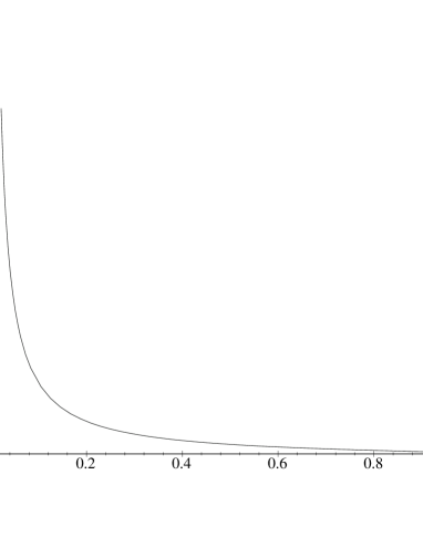
Figure 2: $\frac{\mathfrak{R}(\sigma)T\Lambda}{R^{2}}$ vs. $\sqrt{\frac{U_{0}}{\Lambda}}$

3 Wilson Loops in the Four-Dimensional Background

Let us now turn to the novel four-dimensional background recently obtained in [4]. The metric reads

$$ds^{2}=a(r)\eta_{\mu\nu}dx^{\mu}dx^{\nu}+dr^{2}$$ (31)

where

$$a(r)=\left[\frac{\sqrt{-c_{1}c_{2}}}{c_{1}}\tanh\left(\sqrt{-c_{1}c_{2}}(r+c_{3})\right)\right]^{2/\sqrt{d}}$$ (32)

for $c_{1}$, $c_{2}$ different from $0$, which is the case of interest in the prersent context.

In this background, the induced metric over the world sheet is

$$ds^{2}_{\mbox{ind}}=\left[a(r)(x^{\prime})^{2}+(r^{\prime})^{2}\right]d\sigma^{2}+a(r)(\dot{t})^{2}d\tau^{2}$$ (33)

The Polyakov action is

$$S_{p}=\frac{1}{4\pi\alpha^{\prime}}\int_{M}d^{2}\sigma\left[a(r)\left((x^{\prime})^{2}+(\dot{t})^{2}\right)+(r^{\prime})^{2}\right]$$ (34)

The energy-momentum tensor takes the form

$$j=a(r)\left((x^{\prime})^{2}-(\dot{t})^{2}\right)+(r^{\prime})^{2}$$ (35)

and the momentum

$$p=a(r)x^{\prime}$$ (36)

they follow the relation $j=\frac{p^{2}}{a(r_{0})}-a(r_{0})(\dot{t})^{2}$. We can define $j=\hat{j}a(r_{0})(\dot{t})^{2}$ and $p^{2}=\hat{p}^{2}a(r_{0})^{2}(\dot{t})^{2}$. Conformal invariance implies $\hat{j}=0$ and $\hat{p}^{2}=1$.

Using now the specific value for the warp factor (32) one gets:

$$\sigma=\frac{c_{1}^{1/\sqrt{d}}}{(\dot{t})\left(-c_{1}c_{2}\right)^{(1+\sqrt{d})/(2\sqrt{d})}\tanh^{(1-\sqrt{d})/\sqrt{d}}(v_{0})}\int_{1}^{Y}\frac{y^{(\sqrt{d}-1)/2}dy}{(y^{2}-1)^{1/2}(1-\tanh^{2}(v_{0})y^{\sqrt{d}})}$$ (37)

$$x=\frac{c_{1}^{1/\sqrt{d}}}{\left(-c_{1}c_{2}\right)^{(1+\sqrt{d})/(2\sqrt{d})}\tanh^{(1+\sqrt{d})/\sqrt{d}}(v_{0})}\int_{1}^{Y}\frac{y^{(\sqrt{d}-3)/2}}{(y^{2}-1)^{1/2}(1-\tanh^{2}(v_{0})y^{\sqrt{d}})}$$ (38)

whereas the action is given by:

$$S_{p}=\frac{\left(-c_{1}c_{2}\right)^{(1-2\sqrt{d})/(2\sqrt{d})}T}{2\pi\alpha^{\prime}c_{1}^{1/\sqrt{d}}\tanh^{(1+\sqrt{d})/\sqrt{d}}(v_{0})}\int_{1}^{Y}\frac{y^{(\sqrt{d}+1)/2}dy}{(y^{2}-1)^{1/2}(1-\tanh^{2}(v_{0})y^{\sqrt{d}})}$$ (39)

where $Y=\tanh^{2/\sqrt{d}}(v_{\Lambda})/\tanh^{2/\sqrt{d}}(v_{0})$, and $v_{0}=\sqrt{-c_{1}c_{2}}\frac{\sqrt{d}}{2}r_{0}$, $v_{\Lambda}=\sqrt{-c_{1}c_{2}}\frac{\sqrt{d}}{2}\Lambda$.

In Minkowski signature only the integral condition for $L$ is real, while $\mathfrak{R}(\sigma)$ and $S_{P}$ are complex. We shall work in Euclidean space from now on.

We have not succeeded in solving these integrals in general. When the sources are located in the vicinity of the singularity, (that is when $\Lambda<<l_{s}$, these three integrals can be approximately evaluated by treating the product $by$ as a small quantity, where $b=\tanh(c_{1}r_{0})$. In this case, and working by simplicity in $d=4$, we obtain

$$\mathfrak{R}(\sigma)=\frac{b^{1/2}}{\dot{t}c_{1}}\Bigg{\{}\frac{(Y^{2}-1)^{1/2}(3b^{4}Y^{4}+2b^{2}Y^{2}-10)}{5Y(1-b^{2}Y^{2})}+\left(\frac{3b^{2}}{5}+1\right)\int_{1}^{Y}\frac{z^{1/2}dz}{(z^{-}1)^{1/2}}\Bigg{\}}$$ (40)

$$L=\frac{1}{c_{1}b^{3/2}}\Bigg{\{}\frac{3+19b^{2}-100b^{4}}{3(40b^{4}-36b^{2}+5)}\int_{1}^{Y}\frac{dz}{z^{1/2}(z^{2}-1)^{1/2}}+\hskip 142.26378pt$$

$$+\frac{(Y^{2}-1)^{1/2}[(43-100b^{4})b^{2}Y^{4}+(9-60b^{2})Y^{3}-(10-40b^{2})Y^{2}-(9-60b^{2})]}{3Y^{3/2}(1-b^{2}Y^{2})(40b^{4}-36b^{2}+5)}\Bigg{\}}$$ (41)

and the potential will be

$$V=\frac{1}{2\pi\alpha^{\prime}c_{1}^{2}b^{3/2}}\Bigg{\{}\frac{97b^{2}-55}{3(36b^{2}-40b^{4}+5)}\int_{1}^{Y}\frac{dz}{z^{1/2}(z^{2}-1)^{1/2}}+\hskip 113.81102pt$$

$$+\frac{(Y^{2}-1)^{1/2}[(70-109b^{2})Y^{4}-15Y^{3}-(10-22b^{2})Y^{2}+15]}{Y^{3/2}(1-b^{2}Y^{2})(36b^{2}-40b^{4}-5)}\Bigg{\}}$$ (42)

these results are basically the same one obtains from the confining background of [3], which we have worked out in detail in Appendix A.

A problem with this approximation is that it is not valid when $\Lambda\sim l_{s}$. We can improve on it by building the hyperbolic tangent out of two linear pieces; one corresponding to the confining background, $a=r$, for $r<l_{s}$, and another one $a=1$ for $r\geq l_{s}$

In the region $r>l_{s}$ the background is Minkowskian (Euclidean), and the action is

$$S_{P}=\frac{1}{4\pi\alpha^{\prime}}\int_{M}d^{2}\Sigma\left[(x^{\prime})^{2}+(\dot{t})^{2}+(r^{\prime})^{2}\right]$$ (43)

The conserved quantities associated to this system are

$$p=x^{\prime}$$ (44)

$$q=r^{\prime}$$ (45)

$$j=(r^{\prime})^{2}+(x^{\prime})^{2}-(\dot{t})^{2}$$ (46)

Now conformal invariance implies

$$j=0$$ (47)

$$q=0$$ (48)

$$p=\pm T$$ (49)

The potential between the two heavy sources can now be computed:

$$V=\frac{1}{\pi\alpha^{\prime}}\int_{0}^{L}dx=\frac{1}{\pi\alpha^{\prime}}L$$ (50)

i.e. a linear confining behavior (this is a well-known result; cf. for example [2]).

This behavior can not, however, persist for arbitrarily big values of $\Lambda$ , because there is another string configuration which could be energetically preferred at great values of $\Lambda$ in which the string goes to the origin and comes back to the four dimensional Dirichlet plane. When working directly in the approximation in which the hyperbolic tangent in (32) is replaced by its asymptotic value (that is equivalent to working in flat space), the potential stemming from this configuration is simply

$$V=\frac{\Lambda}{\pi\alpha^{\prime}}$$ (51)

from which it seems clear that when $L$ is much bigger than $\Lambda$ it will be energetivally favored.

Before computing in a more precise way the potential between heavy sources in this configuration, we must check the conditions for this configuration to be a solution of the equations of motion in the background defined by the metric (31). In this case we can work for simplicity in the Nambu-Goto framework. The only condition which appears is

$$x^{\prime}=0$$ (52)

Which when inserted in the equations of motion, yields a condition for $r(\sigma)$, namely,

$$r^{\prime}={\mbox{cotgh}}^{1/2}(c_{1}r)$$ (53)

giving the measure to be used in the computation of the potential, now reading

$$V_{scr}=\frac{1}{\pi\alpha^{\prime}}\int{\mbox{tanh}}^{1/2}(c_{1}r)=\frac{1}{\pi\alpha^{\prime}c_{1}}\left[{\mbox{arctanh}}\left(\sqrt{{\mbox{tanh}}(c_{1}\Lambda)}\right)-{\mbox{arctan}}\left(\sqrt{{\mbox{tanh}}(c_{1}\Lambda)}\right)\right]$$ (54)

We can see a plot of this potential in fig.(3).

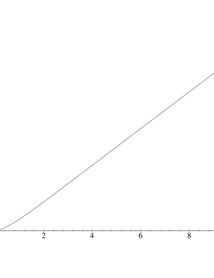
Figure 3: $\pi\alpha^{\prime}c_{1}\,V_{scr}$ vs. $c_{1}\Lambda$

This potential can indeed be approximated at great values of $\Lambda$ as

$$V_{scr}=\frac{(-0.49+0.99c_{1}\Lambda)}{\pi\alpha^{\prime}c_{1}}\approx\frac{\Lambda}{\pi\alpha^{\prime}}$$ (55)

which is basically the same result worked out previously in the Euclidean approximation.

The physical effect of this new configuration is that for any finite value of $\Lambda$, there is a transition from the linear confining phase to a screening behavior of sorts, characterized by a $L$-independent potential, the transition taking place at $L\sim\Lambda$. A similar physical phenomenon appears in the two Wilson loops correlation function at finite temperature ([8]), where beyond certain critical distance determined by the size of the loops, and considering the loops as circles, the correlation itself vanishes, indicating that the new physical configuration consists in a pair of disks.

In this linear approximation there is a change in behavior of the loop according to the value of $\Lambda$. When $\Lambda>l_{s}$ the loop does not penetrate in the bulk, the world sheet remains flat, and the confining behavior is minkowskian (this is what we have just found).

There is, however, a crossover when $\Lambda\sim l_{s}$. Then the loop feels the confining background, penetrates in the bulk, and actually, a new overconfining $L^{3}$ branch appears ([4]). This branch is never energeticaly favored, however, as shown in detail in Appendix A.

From this point of view, the main difference between the four dimensional background presently being studied and the old critical confining one of reference [3] is that now all nontrivial effects appear when $\Lambda<l_{s}$ only, and completely dissapear for $\Lambda>l_{s}$, which corresponds almost exactly to the linear dilaton background.

4 Concluding Remarks

In this paper we have studied the static potential between heavy sources in the new four-dimensional background recently introduced in [3]. The dependence on the value of the holographic coordinate at which the sources lie (which we have called $\Lambda$) has also been studied, and in this particular background there is a crossover at $\Lambda=l_{s}$ from a purely linear behavior towards a region in which a new, cubic branch appears. This branch has got higher energy cost, however.

As a general comment it could perhaps be said, what has been gained with the confining background, or with the purely four-dimensional one, with respect to the simplest of all solutions, namely, the linear dilaton in a flat spacetime?

The answer is twofold: first of all, in order for a holographic interpretation to be consistent in terms of Callan-Symanzik type of renormalization group equations, a mechanism is needed to feed Minkowskian scale transformations on the holographic coordinate, and this looks impossible if the warp factor is trivial ([6]). In the linear dilaton solution it is not possible to interpret the behavior of the dilaton in terms of four dimensional scale transformations $x^{\mu}\rightarrow\lambda x^{\mu}$.

The second reason relies on recent speculations on the closed tachyon potential [13]. From this point of view it seems likely that the confining background is a candidate for the endpoint of tachyon condensation starting from the (unstable) linear dilaton.

The candidate renormalization group flow found in reference [5] precisely starts from linear dilaton in the region where $r=\infty$, in $d=4$, which corresponds to vanishing vacuum expectation value for the tachyon background, $<T>=0$. It then flows to the confining background of reference [3], but also in $d=4$, whereas the original solution was critical, i.e., valid in $d=26$ only. This means that a nonvanishing $<T>\neq 0$ is needed in this region, and this is precisely the characteristic of the flow.

Appendix A Scale Dependence of Wilson Loops in the Confining Background

We are dealing now with a critical bosonic string moving in a background ([3]) given by

$$ds^{2}=\phi d\vec{x}^{2}+l_{c}^{2}d\phi^{2}$$ (56)

where both $x$ and $l_{c}$ have dimensions of length, and $\phi$ has no dimensions.

In order to impose the conformal gauge in the world-sheet, we should work in the isothermal coordinate system, that is, if the induced metric takes the form

$$ds^{2}_{\mbox{ind}}=\left(\phi(x^{\prime})^{2}+l_{c}^{2}(\phi^{\prime})^{2}\right)d\sigma^{2}+\phi\left(\dot{t}\right)^{2}d\tau^{2}$$ (57)

where the prime stands for a derivative with respect to $\sigma$ and the dot with respect to $\tau$, and we have defined $t=t(\tau)$, $\phi=\phi(\sigma)$, $x=x(\sigma)$ and $y=z=0$, we look for a coordinate transformation of the form

$$\frac{d\sigma}{d\xi}=\dot{t}\left(\frac{\phi}{\phi(x^{\prime})^{2}+l_{c}^{2}(\phi^{\prime})^{2}}\right)^{1/2}$$ (58)

and now, in the variables $(\xi,\tau)$, the metric is proportional to the delta.

The Polyakov action in the coordinate system $(\tau,\sigma)$ reads

$$S_{P}=\frac{1}{4\pi l_{s}^{2}}\int d\sigma d\tau\left[\phi(\dot{t})^{2}+\phi(x^{\prime})^{2}+l_{c}^{2}(\phi^{\prime})^{2}\right]$$ (59)

where $\alpha^{\prime}=l_{s}^{2}$ has dimensions of squared length. We can choose $\tau$ and $\sigma$ not to have dimensions, and so we define $t=\tau T$, where now $T$ has dimensions of length.

A conserved quantity comes from the fact that the action does not depend explicitely on $x$, so

$$\phi x^{\prime}=\mbox{constant}\equiv p$$ (60)

otherwise we have the energy-momentum tensor

$$T^{\mu}_{\hskip 5.69046pt\nu}=\frac{\delta\mathfrak{L}}{\delta\partial_{\mu}X^{\rho}}\partial_{\nu}X^{\rho}-\eta^{\mu}_{\hskip 5.69046pt\nu}\mathfrak{L}$$ (61)

which now reads

$$T_{01}=0$$ (62)

$$T_{00}\left(=-T_{11}\right)\equiv j=-\phi T^{2}+\phi(x^{\prime})^{2}+l_{c}^{2}(\phi^{\prime})^{2}$$ (63)

where $p$, in (60), has dimensions of length and $j$, in (63), of squared length.

We will consider a U-shaped string configuration. Denoting by $\phi_{0}$ the tip of this U-shaped string we get

$$j=\frac{p^{2}}{\phi_{0}}-\phi_{0}T^{2}$$ (64)

and

$$\sigma=\frac{l_{c}\phi_{0}^{1/2}}{T}\int_{1}^{Y}\frac{y^{1/2}dy}{\sqrt{(y-1)(y+\hat{p}^{2})}}$$ (65)

this can be written for the coordinate $\xi$ as

$$\xi=\frac{l_{c}\phi_{0}^{1/2}}{T}\int_{1}^{Y}\frac{(y+\hat{j})^{1/2}dy}{\sqrt{(y-1)(y+\hat{p}^{2})}}$$ (66)

where we have defined $j=\hat{j}\phi_{0}T^{2}$ and $p^{2}=\hat{p}^{2}\phi_{0}^{2}T^{2}$ so they follow the relation

$$\hat{j}=\hat{p}^{2}-1$$ (67)

Now we can use (65) to get from (60)

$$x=l_{c}\hat{p}\phi_{0}^{1/2}\int_{1}^{Y}\frac{dy}{\sqrt{y(y-1)(y+\hat{p}^{2})}}$$ (68)

Imposing Dirichlet boundary conditions at the codimension one hypersurface $\phi=\Lambda$, so we get from (65) and (68)

$$\mathfrak{R}(\xi)=\frac{2l_{c}\phi_{0}^{1/2}}{T}\int_{1}^{\sqrt{\Lambda/\phi_{0}}}\sqrt{\frac{\chi^{2}(\chi^{2}+\hat{j})}{(\chi^{2}-1)(\chi^{2}+\hat{p}^{2})}}d\chi$$ (69)

where $\mathfrak{R}(\xi)$ is defined through $0\leq\xi\leq\mathfrak{R}(\xi)$, and the physical separation of the heavy sources (which is the only external data) must be now be fed through:

$$L=\int_{0}^{\mathfrak{R}(\xi)}\frac{dx}{d\xi}d\xi$$ (70)

that is,

$$L=2l_{c}\hat{p}\phi_{0}^{1/2}\int_{1}^{\sqrt{\Lambda/\phi_{0}}}\frac{d\chi}{\sqrt{(\chi^{2}-1)(\chi^{2}+\hat{p}^{2})}}$$ (71)

The action, in isothermal coordinates, is then given by

$$S=\frac{\hat{j}l_{c}t\phi_{0}^{3/2}}{2\pi l_{s}^{2}}\int_{1}^{\sqrt{\Lambda/\phi_{0}}}\sqrt{\frac{\chi^{2}(\chi^{2}+\hat{j})(2\chi^{2}+\hat{j})^{2}}{(\chi^{2}-1)(\chi^{2}+\hat{p}^{2})}}d\chi$$ (72)

Before trying to solve these equations we have got one extra condition for conformal invariance, that is the vanishing of the energy-momentum tensor. This condition can be seen as

$$\hat{j}=0$$

$$\hat{p}^{2}=1$$ (73)

with these two conditions one can write (69), (71) and (72) as

$$\mathfrak{R}(\xi)=\mathfrak{R}(\sigma)=\frac{2l_{c}\phi_{0}^{1/2}}{T}\int_{1}^{\sqrt{\Lambda/\phi_{0}}}\frac{\chi^{2}d\chi}{\sqrt{\chi^{4}-1}}$$ (74)

$$L=\pm 2l_{c}\phi_{0}^{1/2}\int_{1}^{\sqrt{\Lambda/\phi_{0}}}\frac{d\chi}{\sqrt{\chi^{4}-1}}$$ (75)

$$S=\frac{l_{c}t\phi_{0}^{3/2}}{\pi l_{s}^{2}}\int_{1}^{\sqrt{\Lambda/\phi_{0}}}\frac{\chi^{4}d\chi}{\sqrt{\chi^{4}-1}}$$ (76)

These integrals can be solved in terms of elliptic functions as

$$\mathfrak{R}(\sigma)=\frac{2l_{c}\phi_{0}^{1/2}}{T}\left[\frac{\sqrt{2}}{2}F\left(\cos^{-1}\sqrt{\frac{\phi_{0}}{\Lambda}},\frac{1}{\sqrt{2}}\right)-\sqrt{2}E\left(\cos^{-1}\sqrt{\frac{\phi_{0}}{\Lambda}},\frac{1}{\sqrt{2}}\right)+\sqrt{\frac{\phi_{0}}{\Lambda}}\sqrt{\frac{\Lambda^{2}}{\phi_{0}^{2}}-1}\right]$$ (77)

$$L=\pm 2l_{c}\phi_{0}^{1/2}\frac{1}{\sqrt{2}}F\left(\cos^{-1}\sqrt{\frac{\phi_{0}}{\Lambda}},\frac{1}{\sqrt{2}}\right)$$ (78)

$$S=\frac{l_{c}T\phi_{0}^{3/2}}{\pi l_{s}^{2}}\left[\frac{1}{3\sqrt{2}}F\left(\cos^{-1}\sqrt{\frac{\phi_{0}}{\Lambda}},\frac{1}{\sqrt{2}}\right)+\frac{1}{3}\sqrt{\frac{\phi_{0}}{\Lambda}}\sqrt{\frac{\Lambda^{2}}{\phi_{0}^{2}}-1}\right]$$ (79)

This leads to essentially the same equations than those in [4], taking into account the $1/4\pi$ factors in the definition of the Polyakov action and the $1/2\pi$ in the Nambu-Goto one, but we also obtain another extra condition, namely, that of (77). Together, these three equations imply that

$$S=\frac{TE\left(\cos^{-1}\sqrt{\frac{\phi_{0}}{\Lambda}},\frac{1}{\sqrt{2}}\right)}{6\pi l_{s}^{2}l_{c}^{2}F^{3}\left(\cos^{-1}\sqrt{\frac{\phi_{0}}{\Lambda}},\frac{1}{\sqrt{2}}\right)}L^{3}+$$

$$+\frac{TL^{2}}{12\pi l_{s}^{2}l_{c}^{2}F^{2}\left(\cos^{-1}\sqrt{\frac{\phi_{0}}{\Lambda}},\frac{1}{\sqrt{2}}\right)}\left(T\mathfrak{R}(\sigma)-2l_{c}\Lambda^{1/2}\sqrt{1-\frac{\phi_{0}^{2}}{\Lambda^{2}}}\right)+\frac{Tl_{c}\Lambda^{3/2}}{3\pi l_{s}^{2}}\sqrt{1-\frac{\phi_{0}^{2}}{\Lambda^{2}}}$$

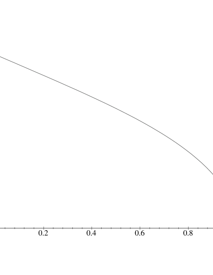
Figure 4: $T\mathfrak{R}(\sigma)/l_{c}\sqrt{\Lambda}$ vs. $\sqrt{\phi_{0}/\Lambda}$

Before trying to extract any conclusion from this expression, we may see what (77) is telling.

From this equation we can read a relation between $T\mathfrak{R}(\sigma)/l_{c}\sqrt{\Lambda}$ and $\sqrt{\phi_{0}/\Lambda}$, plotted in fig.(4). This relation sets the range of $\sigma$ as

$$0\leq\frac{\mathfrak{R}(\sigma)}{\Lambda^{1/2}}\leq\frac{2l_{c}}{T}$$ (81)

so, in the limit $\Lambda\rightarrow\infty$, this variable diverges. This divergence is also present in (A), but is exactly cancelled, so in this limit we find the following relation for the potential between heavy sources:

$$V=\frac{E(1/\sqrt{2})}{3\pi l_{s}^{2}l_{c}^{2}K(1/\sqrt{2})^{3}}L^{3}+\frac{2l_{c}\Lambda^{3/2}}{3\pi l_{s}^{2}}$$ (82)

So we find an over confinig region and two different divergences, but only one of them is present in the potential.

Now we can compute the potential in the limit $\Lambda\approx\phi_{0}$. In a naïve way one obtains

$$V=\frac{L\Lambda}{3\pi l_{s}^{2}}$$ (83)

i.e. a linear confining behaviour.

There is another interesting relation, that of (78). This equation give us the relation between $\sqrt{\frac{\phi_{0}}{\Lambda}}$ and $\frac{L}{l_{c}\sqrt{\Lambda}}$. This is plotted is fig.(5) and tell us that for each $L$, there are two possible configurations, which we will call regions $I$ and $II$ ([4][9]).

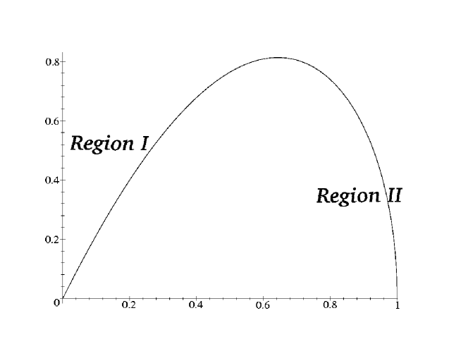
Figure 5: Relation between $x=\sqrt{\frac{\phi_{0}}{\Lambda}}$ and $y=\frac{L}{l_{c}\sqrt{\Lambda}}$

In order to guess which configuration is in, favored energetically we have to look for analytic (up to an order of magnitude) expressions of the equations (77-79). Firstly we expand the elliptic functions as

$$F(\cos^{-1}(x),1/\sqrt{2})=\frac{2}{\pi}K(1/\sqrt{2})\left[\cos^{-1}(x)-x\sqrt{1-x^{2}}\left(\frac{5}{3}-\frac{2}{3}x^{2}\right)\right]+\hskip 14.22636pt$$

$$+x\sqrt{1-x^{2}}\left(\frac{7}{4}-\frac{3}{4}x^{2}\right)$$ (84)

$$E(\cos^{-1}(x),1/\sqrt{2})=\frac{2}{\pi}E(1/\sqrt{2})\left[\cos^{-1}(x)-x\sqrt{1-x^{2}}\left(\frac{5}{3}-\frac{2}{3}x^{2}\right)\right]+\hskip 14.22636pt$$

$$+x\sqrt{1-x^{2}}\left(\frac{19}{12}-\frac{7}{12}x^{2}\right)$$ (85)

with these two equations we can invert (78). We obtain four solutions to the equation, but only two of them are physically relevant. These are

$$\left(\frac{\phi_{0}^{(1)}}{\Lambda}\right)^{1/2}=\frac{5}{4}+\frac{1}{12}\sqrt{B}-\frac{1}{12}\sqrt{6}\sqrt{\frac{43A^{1/3}\sqrt{B}-A^{2/3}\sqrt{B}+36\sqrt{B}z^{2}-64\sqrt{B}+405A^{1/3}}{A^{1/3}\sqrt{B}}}$$ (86)

$$\left(\frac{\phi_{0}^{(2)}}{\Lambda}\right)^{1/2}=\frac{5}{4}-\frac{1}{12}\sqrt{B}+\frac{1}{12}\sqrt{6}\sqrt{\frac{43A^{1/3}\sqrt{B}-A^{2/3}\sqrt{B}+36\sqrt{B}z^{2}-64\sqrt{B}+405A^{1/3}}{A^{1/3}\sqrt{B}}}$$ (87)

where $z=\frac{L}{l_{c}\Lambda^{1/2}}$, and

$$A=-1161z^{2}+512+9\sqrt{576z^{6}+13569z^{4}-9216z^{2}}$$ (88)

$$B=-\frac{-129A^{1/3}-6A^{2/3}+216z^{2}-384}{A^{1/3}}$$ (89)

each solution corresponds to one of the two regions in fig.(5), namely, (86) corresponds to region I, while (87) corresponds to region II.

An important feature of these solutions is that they are valid in all the range of $\phi_{0}\leq\phi\leq\Lambda$. Given this, we can write down an expression for the potential valid in all the range of $\phi_{0}\leq\phi\leq\Lambda$ for each region. This is given by

$$\frac{3\pi l_{s}^{2}}{2l_{c}\Lambda^{3/2}}V^{(1)}=\sqrt{1-\left(\frac{5}{4}+\frac{\sqrt{B}}{12}-\frac{C_{+}}{12}\right)^{4}}+\frac{\sqrt{3}}{3}\left(\frac{5}{4}+\frac{\sqrt{B}}{12}-\frac{C_{+}}{12}\right)^{3}\times$$ (90)

$$\times\sqrt{\left(\frac{5}{4}+\frac{\sqrt{B}}{12}-\frac{C_{+}}{12}\right)^{2}-\frac{9}{4}-\frac{5\sqrt{B}}{12}+\frac{5C_{+}}{12}}$$ (91)

for region I, and

$$\frac{3\pi l_{s}^{2}}{2l_{c}\Lambda^{3/2}}V^{(2)}=\sqrt{1-\left(\frac{5}{4}-\frac{\sqrt{B}}{12}+\frac{C_{-}}{12}\right)^{4}}+\frac{\sqrt{3}}{3}\left(\frac{5}{4}-\frac{\sqrt{B}}{12}+\frac{C_{-}}{12}\right)^{3}\times$$ (92)

$$\times\sqrt{\left(\frac{5}{4}-\frac{\sqrt{B}}{12}+\frac{C_{-}}{12}\right)^{2}-\frac{9}{4}+\frac{5\sqrt{B}}{12}-\frac{5C_{-}}{12}}$$ (93)

for region II. Where $A$ and $B$ are given by (88) and (89) respectively and

$$C_{\pm}=\sqrt{6}\sqrt{\frac{43A^{1/3}\sqrt{B}-A^{2/3}\sqrt{B}+36\sqrt{B}z^{2}-64\sqrt{B}\pm 405A^{1/3}}{A^{1/3}\sqrt{B}}}$$ (94)

These solutions are plotted in fig.(6). From this plot we can see that to region II corresponds a smaller potential energy.

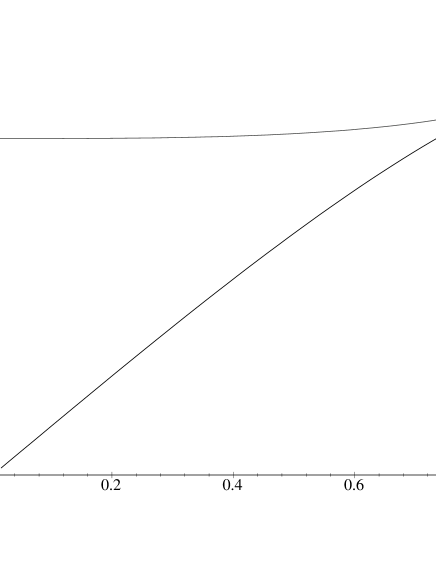
Figure 6: $j\bar{j}$ potential corresponding to the two available configurations. The plot is $\frac{3\pi l_{s}^{2}}{2l_{c}\Lambda^{3/2}}V$ vs. $\frac{L}{l_{c}\Lambda^{1/2}}$

An interesting feature of this plot is that the potential corresponding to the linear confining region does not reach the point $L=0$. This can be interpreted as follows.

Looking at fig.(5), it is apparent that there are two critical points in the holographic direction: $\phi_{0}=0$ and $\phi_{0}=\infty$, however, in view of fig.(5), we can see that there is another one, the corresponding to the maximun in that figure. This point corresponds to the maximun potential energy available between the two sources, that is, to the point of maximun possible separation between the two sources.

This presumably means that this is the point where a new pair $j\bar{j}$ is created.

The two regions in fig.(5) correspond to both sides of the critical plane just defined. The distance between the sources decreases as we move away from this plane.

In this way, as we approach $\phi_{0}=0$, we move towards $L=0$. However, in this limit, the metric is singular, so we can never reach $L=0$ in this way. In fact the string, through $\phi_{0}$, would go into the singularity before we reach it, through $\Lambda$.

This is what makes this configuration of region $II$ disappear, leaving us with just region $I$, as $\Lambda\rightarrow\infty$.

There is however in this limit another point that must be clarified.

In the body of the paper, we have demonstrated that the equations of motion that arise from Nambu-Goto and Polyakov actions are the same, being this last written in the isothermal coordinate system. However, in the Polyakov’s case we found an extra condinition, namely, that of $\sigma$. This condition plays a role more important than been merely a parametrization of the world-sheet.

The divergence in $\sigma$, as seen from eq.(77), makes the finite part of the potential in eq.(82) to be different from the one computed in [4]. This fact does not point to a contradiction, however. One must simply have in mind that the equivalence of the equations of motion coming from different lagrangians is due to the fact that one can always add a total derivative of a function of position and time to the old lagrangian.

When saying this one always assumes that such a function is well behaved at the boundaries. Now this is not the case, because in the boundaries is where we are in trouble: a geometric singularity at the origin and a divergent coupling constant at the infinity of the holographic coordinate.

Appendix B Detailed Analysis of some Supergravity Solutions

It is intesting to consider related backgrounds which, although not conformal, appear naturally in the context of supergravity. Let us choose as an example the one in reference [12]. This background is given by

$$ds^{2}=y^{1/2}d\vec{x}^{2}+Ady^{2}$$ (95)

The induced metric will be

$$ds^{2}_{\mbox{ind}}=\left[y^{1/2}(x^{\prime})^{2}+A(y^{\prime})^{2}\right]d\sigma^{2}+y^{1/2}(\dot{t})^{2}d\tau^{2}$$ (96)

so the Polyakov action is

$$S_{P}=\frac{1}{4\pi\alpha^{\prime}}\int_{M}d^{2}\Sigma\Big{\{}y^{1/2}\left[(x^{\prime})^{2}+(\dot{t})^{2}\right]+A(y^{\prime})^{2}\Big{\}}$$ (97)

The change of variables that should be done in order to compute in the isothermal coordinate system will be

$$\frac{d\sigma}{d\xi}=T\frac{y^{1/4}}{\left[j+y^{1/2}T^{2}\right]^{1/2}}$$ (98)

where $j$ is again the ”$00$” component of the energy-momentum tensor obtained from the action (97)

$$j=y^{1/2}\left[(x^{\prime})^{2}-(\dot{t})^{2}\right]+A(y^{\prime})^{2}$$ (99)

the other conserved quantitie associated to (97) is

$$p=y^{1/2}x^{\prime}$$ (100)

from these two quantities we can define a new set of constants

$$j=\hat{j}y_{0}^{1/2}T^{2}$$ (101)

$$p^{2}=\hat{p}^{2}y_{0}T^{2}$$ (102)

where $y_{0}$ is defined, as is customary, as the tip of the U-shaped string configuration. Conformal invariance implies

$$\hat{j}=0$$ (103)

$$\hat{p}^{2}=1$$ (104)

Now we are ready to construct the constraint conditions to the parametrization of the world-sheet and to the lenght of the wilson loop as

$$\mathfrak{R}(\xi)=\frac{4A^{1/2}y_{0}^{3/4}}{T}\int_{1}^{(\Lambda/y_{0})^{1/4}}\frac{\chi^{4}d\chi}{\left[(\chi^{2}-1)(\chi^{2}+1)\right]^{1/2}}$$ (105)

$$L=4A^{1/2}y_{0}^{3/4}\int_{1}^{(\Lambda/y_{0})^{1/4}}\frac{\chi^{2}d\chi}{\left[(\chi^{2}-1)(\chi^{2}+1)\right]^{1/2}}$$ (106)

and the action is

$$S_{P}=\frac{2TA^{1/2}y_{0}^{5/4}}{\pi}\int_{1}^{(\Lambda/y_{0})^{1/4}}\frac{\chi^{6}d\chi}{\left[(\chi^{2}-1)(\chi^{2}+1)\right]^{1/2}}$$ (107)

Figure 7: $\frac{3T\mathfrak{R}(\sigma)}{4A^{1/2}\Lambda^{3/4}}$ vs. $\left(\frac{y_{0}}{\Lambda}\right)^{1/4}$

These three integrals can be solved as

$$\mathfrak{R}(\xi)=\frac{4A^{1/2}y_{0}^{3/4}}{3T}\left\{\frac{1}{\sqrt{2}}F\left(\arccos\left(\frac{y_{0}}{\Lambda}\right)^{1/2},\frac{1}{\sqrt{2}}\right)+\frac{\Lambda^{3/4}}{y_{0}^{3/4}}\sqrt{1-\frac{y_{0}}{\Lambda}}\right\}$$ (108)

$$L=4A^{1/2}y_{0}^{3/4}\left\{\frac{1}{\sqrt{2}}F\left(\arccos\left(\frac{y_{0}}{\Lambda}\right)^{1/2},\frac{1}{\sqrt{2}}\right)-\sqrt{2}E\left(\arccos\left(\frac{y_{0}}{\Lambda}\right)^{1/2},\frac{1}{\sqrt{2}}\right)+\frac{\Lambda^{1/4}}{y_{0}^{1/4}}\sqrt{1-\frac{y_{0}}{\Lambda}}\right\}$$ (109)

$$S_{P}=\frac{2TA^{1/2}y_{0}^{5/4}}{5\pi l_{s}^{2}}\Biggr{\{}\frac{3}{\sqrt{2}}F\left(\arccos\left(\frac{y_{0}}{\Lambda}\right)^{1/2},\frac{1}{\sqrt{2}}\right)-3\sqrt{2}E\left(\arccos\left(\frac{y_{0}}{\Lambda}\right)^{1/2},\frac{1}{\sqrt{2}}\right)+$$

$$+3\frac{\Lambda^{1/4}}{y_{0}^{1/4}}\sqrt{1-\frac{y_{0}}{\Lambda}}+\frac{\Lambda^{5/4}}{y_{0}^{5/4}}\sqrt{1-\frac{y_{0}}{\Lambda}}\Biggr{\}}$$ (110)

In the limit $\Lambda\approx y_{0}$ we can find the following behaviour

$$V=\frac{3L\Lambda^{1/2}}{5\pi l_{s}^{2}}$$ (111)

Figure 8: $\frac{L}{4A^{1/2}\Lambda^{3/4}}$ vs. $\left(\frac{y_{0}}{\Lambda}\right)^{1/4}$

The first thing one may say about this background is that it, basically, give us the same kind of configurations seen in the last section. First of all, the range of $\xi$ is read from fig.(7). This is

$$0\leq\frac{\mathfrak{R}(\xi)}{\Lambda^{3/4}}\leq\frac{4A^{1/2}}{3T}$$ (112)

This behaviour of $\sigma$ allow us to write the potential when $\Lambda\rightarrow\infty$ as

$$V=\frac{4A^{1/2}}{5\pi\lambda_{s}^{2}}\Lambda^{5/4}$$ (113)

Secondly, the string can live in two possible configurations as seen in fig.(8)

Now we want to say which configuration costs less energy. In order to do so, we should invert eq.(109), as in the previous section. However, in this case, the more we can do is an interpolation to get a polynomial solution. Once again, the region corresponding to a linear confining region is the physically relevant. This turns out to be

$$\frac{5\pi l_{s}^{2}}{4A^{1/2}\Lambda^{5/4}}V=(1+3\Delta^{4})\sqrt{1-\Delta^{4}}-3\Delta^{5}\sqrt{\Delta-\Delta^{2}}$$ (114)

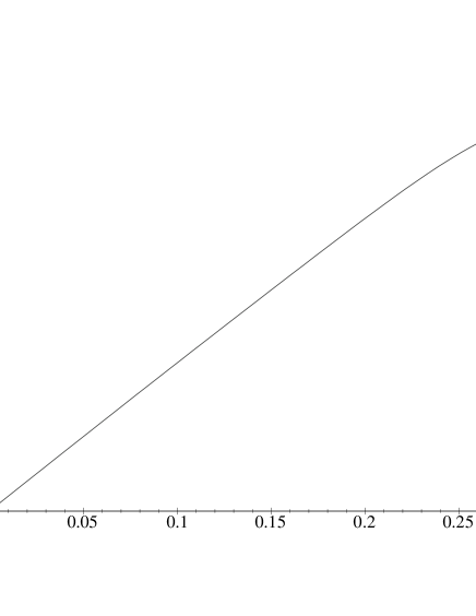
Figure 9: $\frac{5\pi l_{s}^{2}}{4A^{1/2}\Lambda^{5/4}}V$ vs. $\frac{L}{4A^{1/2}\Lambda^{1/4}}$

where $\Delta$ is given, approximately, by

$$\Delta=-129.22z^{6}+19.18z^{5}-5.33z^{4}+0.42z^{3}-z^{2}+0.28\times 10^{-5}z+1$$ (115)

where $z=\frac{L}{4A^{1/2}\Lambda^{1/4}}$.

This potential is given in fig.(9). There are a few comments to be made. First of all we see that the potential is linear in the product $L\Lambda^{1/2}$, corresponding to the so called region $II$. However, in this case we cannot see the effect of the singularity in the origin, due to the interpolation we made, altough it is expected to cause similar problems as with the confining background.

References

[1] O. Aharony, S. S. Gubser, J. Maldacena, H. Ooguri, Y. Oz,
Large N Field Theories, String Theory and Gravity,
hep-th/9905111
[2] Orlando Alvarez,
The Static Potential In String Models,
Phys. Rev. D24 (1981) 440.
[3] E. Alvarez and C. Gomez,
The confining string from the soft dilaton theorem,
Nucl. Phys. B566 (2000) 363
hep-th/9907158
[4] E. Álvarez and C. Gómez,
On the string description of confinement,
jhep05 (2000) 012, hep-th/0003205
[5] E. Alvarez, C. Gomez and L. Hernandez,
Non-Critical Poincaré Invariant Bosonic
String Backgrounds and Closed String Tachyons,
hep-th/0011105.
[6] E. Alvarez and C. Gomez,
Non-critical confining strings and the renormalization
group,
Nucl. Phys. B550 (1999) 169,hep-th/9902012.
J. de Boer, E. Verlinde and H. Verlinde,
On the holographic renormalization group,
JHEP 0008 (2000) 003
hep-th/9912012.
E. Alvarez and C. Gomez,
A comment on the holographic renormalization group
and the soft dilaton theorem,
Phys. Lett. B476 (2000) 411,hep-th/0001016.
[7] M.B.Green.J.H.Schwarz and E. Witten,
Superstring Theory(Cambridge University Press,1987)
[8] D.J.Gross and H.Ooguri
Aspects of Large N Gauge Theory Dynamics as Seen by
String Theory,hep-th/9805129.
A.Brandhuber, N.Itzhaki, J.Sonnenschein and S.Yankielowicz,
Wilson Loops in the Large N Limit at Finite Temperature,
hep-th/9803127.
S.Rey, S.Theisen and J.Yee,
Wilson-Polyakov Loop at Finite Temperature in Large N
Gauge Theory and Anti-de Sitter Supergravity,
hep-th/9803125
[9]
I. Kogan, M. Schvellinger and B. Tekin,
Holographic renormalization group flow, Wilson loops and
field-theory beta-functions,
Nucl. Phys. B588 (2000) 213
hep-th/0004185.
[10] J. Maldacena,
The large N limit of superconformal field
theories and supergravity,
Adv. Theor. Math. Phys. 2 (1998) 231
hep-th/9711200.
[11] J. Maldacena,
Wilson loops in large N field theories,
hep-th/9803002 S. Rey and J. Yee,
Macroscopic strings as heavy quarks in large
N gauge theory and anti-de Sitter supergravity,
hep-th/9803001.
[12] M. Porrati and A. Starinets
RG fixed points in supergravity duals of 4-d
field theory and asymptotically AdS spaces,
Phys. Lett. B454 (1999) 77
hep-th/9903085.
[13]A. Sen,
Universality of the tachyon potential,
JHEP 9912 (1999) 027
hep-th/9911116.
J. A. Harvey, D. Kutasov and E. J. Martinec,
On the relevance of tachyons,
hep-th/0003101.
D. Kutasov, M. Mariño and G. Moore,
Some exact results on tachyon condensation in string field theory,
hep-th/0009148.
[14] J. Sonnenschein,
What does the string / gauge correspondence
teach us about Wilson loops?,
hep-th/0003032.
[15] M. Spivak,
A Comprehensive Introduction to Differential
geometry, vol. II(Publish or Perish)
[16] E.Witten
Anti-de Sitter space and holography,
Adv. Theor. Math. Phys. 2 (1998) 253
hep-th/9802150.
Anti-de Sitter space, thermal phase transition,
and confinement in gauge theories,
Adv. Theor. Math. Phys. 2 (1998) 505
hep-th/9803131.