Abstract

We present the results of a numerical investigation of percolation properties in a version of the classical Heisenberg model. In particular we study the percolation properties of the subsets of the lattice corresponding to equatorial strips of the target manifold ${\cal S}^{2}$. As shown by us several years ago, this is relevant for the existence of a massless phase of the model. Our investigation yields strong evidence that such a massless phase does indeed exits. It is further shown that this result implies lack of asymptotic freedom in the massive continuum limit. A heuristic estimate of the transition temperature is given which is consistent with the numerical data.

PACS: 64.60.Cn, 05.50.+q, 75.10.Hk

1 Introduction

If one looks at textbooks to learn about the phase diagram of the two dimensional ($2D$) $O(N)$ models the situation seems clear: for $N=2$, there is a transition to a low temperature phase with only power law decay of correlations, whereas for the nonabelian case $N>2$ there is exponential decay at all temperatures. But while the first statement has been proven rigorously a long time ago [1], the second one remains an open mathematical question [2]. The standard belief is rooted in the perturbative asymptotic freedom of the models for $N>2$; but over the years we have brought forth many reasons why we think it is unfounded [3, 4, 5]. The absence of a mathematical proof together with ambiguous numerical results left the issue wide open.

In this paper we would like to present what we regard as convincing numerical evidence that in fact the $2D$ $O(3)$ model possesses a massless phase for sufficiently large $\beta$ and give a rigorous proof that this is incompatible with asymptotic freedom in the massive phase. We will also give a heuristic explanation of why and where the phase transition happens.

The models we are considering consist of classical spins $s$ taking values on the unit sphere $S^{N-1}$, placed at the sites of a $2D$ regular lattice. These spins interact ferromagnetically with their nearest neighbors. Let $\langle ij\rangle$ denote a pair of neighboring sites. We will consider two types of interactions between neighbouring spins:

• Standard action (s.a.): $H_{ij}=-s(i)\cdot s(j)$

• Constrained action (c.a.): $H_{ij}=-s(i)\cdot s(j)$ for $s(i)\cdot s(j)\geq c$ and $H_{ij}=\infty$ for $s(i)\cdot s(j)<c$ for some $c\in[-1,1)$.

The corresponding Gibbs measures are (for a finite lattice) given by

$$d\mu_{s.a.}={1\over Z}\prod_{\langle ij\rangle}e^{-\beta H_{ij}}\prod_{i}d\nu\left(s(i)\right)$$ (1)

for the standard action and

$$d\mu_{c.a.}={1\over Z}\prod_{\langle ij\rangle}\left[e^{-\beta H_{ij}}\theta\left(s(i)\cdot s(j)-c\right)\right]\prod_{i}d\nu\left(s(i)\right)$$ (2)

for the constrained action, where $d\nu$ is the standard measure on the two sphere $S^{2}$ and the product $\prod_{\langle ij\rangle}$ is over nearest neighbors.

Almost a decade ago we showed [6] that one can rephrase the question of the existence of a soft phase in these models as a percolation problem and in fact this is the reason we introduced the c.a. model. It should be noted that the c.a. model shares with the s.a. model not only invariance under $O(N)$, but has also the same perturbative (= low temperature) expansion and the same ‘smooth’ classical solutions as the s.a. model. It is therefore to be expected that the s.a. and c.a. models fall in the same universality class (possess the same continuum limit) and, as we shall show shortly, the numerical evidence supports this expectation. The advantage of studying the c.a. model stems from the following fact: let $\epsilon_{c}=\sqrt{2(1-c)}$ and $S_{\epsilon_{c}}$ the set of sites such that $|s\cdot n|<\epsilon_{c}/2$ for some given unit vector $n$. Our rigorous result [6] was that if for some $\epsilon>\epsilon_{c}$ the set $S_{\epsilon}$ on the triangular (T) lattice does not contain a percolating cluster, then the $O(N)$ model must be massless at that $c$. For the abelian $O(2)$ model we could prove the absence of percolation of this equatorial set $S_{\epsilon_{c}}$ for $c$ sufficiently large [6] (modulo certain technical assumptions which were later eliminated by M. Aizenman [7]). For the nonabelian cases we could not give a rigorous proof. We did however present certain arguments [8, 9] explaining why the percolating scenario seemed unlikely.

In this paper we will present numerical evidence that there is an $\epsilon_{)}$ such that for $\epsilon\leq\epsilon_{0}$ $S_{\epsilon}$ does not percolate for any $c$; for sufficiently large $c$ this $\epsilon_{0}$ will be larger than $\epsilon_{c}$ and the model will thus be massless. We will also show that due to a rigorous inequality derived by us in the past [10], the existence of a finite $\beta_{crt}$ in the s.a. model on the square (S) lattice is incompatible with the presence of asymptotic freedom in the massive continuum limit of the model.

2 Percolation and masslessness

In this section we briefly review the special features of percolation in two dimensions and give a brief sketch of our argument relating percolation properties to the absence of a mass gap. We restrict the discussion to the T lattice; this keeps the arguments simpler because the T lattice is self-matching and no distinction has to be made between connectedness and $\star$-connectedness (where points are also considered connected along diagonals).

The following two facts special to $2D$ are relevant for our discussion:

1. Noncoexistence of disjoint percolating sets: Let $A$ be the subset of the lattice defined by the spin lying in some subset ${\cal A}\subset S^{N-1}$ and $\tilde{A}$ its complement. Then with probability 1 $A$ and $\tilde{A}$ do not percolate at the same time. This has been proven rigorously only for special cases like Bernoulli percolation and the $+$ and $-$ clusters of the Ising model, but is believed to hold quite generally. (Aizenman [7] showed that in the case of $O(2)$ one does not need to invoke this principle).

2. Russo’s lemma [11]: If neither $A$ nor its complement $\tilde{A}$ percolate, then the expected size of the cluster of $A$ attached to the origin, denoted by $\langle A\rangle$, diverges; the same holds for its complement $\tilde{A}$. (In this simple form the lemma only holds for a self matching lattice like the T lattice). If $\tilde{A}$ percolates, then $\langle A\rangle$ is expected to be finite.

The subsets of the sphere $S^{2}$ that interest us here are the following:

• ‘equatorial strip’ ${\cal S}_{\epsilon}$, defined by $|s\cdot n|<\epsilon/2$ for some fixed unit vector $n$.

• ‘upper polar cap’ ${\cal P}_{\epsilon}^{+}$, defined by $s\cdot n\geq\epsilon/2$,

• ‘lower polar cap’ ${\cal P}_{\epsilon}^{-}$, defined by $s\cdot n\leq-\epsilon/2$.

• ‘union of polar caps’ ${\cal P}_{\epsilon}={\cal P}_{\epsilon}^{+}\cup{\cal P}_{\epsilon}^{-}$.

The subsets of the lattice defined by these subsets of the sphere we denote by the corresponding roman letters $S_{\epsilon}$ etc. and for brevity we say ‘a certain subset of the sphere percolates’ instead of ‘the subset of the lattice induced by a certain subset of the sphere percolates’ etc..

According to the discussion above, there are the following possibilities: either $S_{\epsilon}$ percolates, or $P_{\epsilon}$ percolates, or neither $S_{\epsilon}$ nor $P_{\epsilon}$ percolates and then both have divergent mean size (we shall call this third possibility in short formation of rings).

Let us now briefly review our argument [6] that relates percolation properties to the absence of a mass gap. Our statement was that if there was an equatorial strip ${\cal S}_{\epsilon}$ that did not percolate for a certain $c>1-\epsilon^{2}/2$, there could be no mass gap in the system.

The argument is based on the imbedded Ising variables $\sigma_{i}\equiv{\rm sgn}(s(i))$. Using these variables, the s.a. Hamiltonian becomes:

$$H_{ij}=-\sigma_{i}\sigma_{j}|s_{\|}(i)s_{\|}(j)|-s_{\perp}(i)\cdot s_{\perp}(j)$$ (3)

where $s_{\|}(i)=s(i)\cdot n$ and $s_{\perp}(i)=n\times(s(i)\times n)$. The c.a. model can be similarly described in terms of the variables $\sigma_{i}$, $|s_{\|}(i)|$ and $s_{\perp}(i)$. In both models one thus obtains an induced Ising model for which the Fortuin-Kastleyn (FK) representation [12] is applicable. In this representation the Ising system is mapped into a bond percolation problem: In the s.a. model a bond is placed between any like neighboring Ising spins with probability $p=1-\exp(-2\beta s_{\|}(i)s_{\|}(j))$. For the c.a. model a bond is also placed if after flipping one of the two neighboring Ising spins the constraint $s(i)\cdot s(j)\geq c$ is violated. From the FK representation is follows that the mean cluster size of the site clusters joined by occupied bonds (FK-clusters) is equal to the Ising magnetic susceptibility. In a massive phase the latter must remain finite. Hence, if the FK-clusters have divergent mean size, the original $O(3)$ ferromagnet must be massless (the Ising variables $\sigma$ are local functions of the originally spin variables $s$).

Now notice that by construction for the c.a. model the FK-clusters with, say, $\sigma=+1$ must contain all sites with $s(i)\cdot n>\sqrt{(1-c)/2}$. Therefore the model must be massless if clusters obeying this condition have divergent mean size. But the polar set $P_{\epsilon}$ consists of the two disjoint components $P^{+}_{\epsilon}$ and $P^{-}_{\epsilon}$. For $c>1-\epsilon^{2}/2$ there are no clusters containing elements of both $P^{+}_{\epsilon}$ and $P^{-}_{\epsilon}$. Hence if for such values of $c$ clusters of $P_{\epsilon}$ form rings, so do clusters of $P^{+}_{\epsilon}$ separately and the $O(3)$ model must be massless by the argument just given.

If we want to study the percolation or absence of percolation of the set $A$ corresponding to a subset ${\cal A}\subset S^{N-1}$ of positive measure numerically, we have to consider a sequence of tori of increasing size $L$. On these tori we measure the mean cluster size of of $A$. If $A$ percolates in the thermodynamic limit, by translation invariance $\langle A\rangle=O(L^{2})$; if its complement percolates $\langle A\rangle$ should approach a finite nonzero value, and if $A$ forms rings we expect $\langle A\rangle=O(L^{2-\eta})$ for some $\eta>0$. Therefore, if we define the ratio

$$r=\langle P_{\epsilon}\rangle/\langle S_{\epsilon}\rangle,$$ (4)

for $L\to\infty$ it should either go to 0 if $S_{\epsilon}$ percolates or to $\infty$ if $P_{\epsilon}$ percolates; if neither $S_{\epsilon}$ nor $P_{\epsilon}$ percolates, then both form rings and the ratio $r$ could diverge, go to 0 or approach some finite, nonzero value depending upon the value of the critical index $\eta$ for the two types of clusters.

In the next section we will describe what our numerical simulations tell us about the percolation properties of equatorial strips and polar caps.

3 Main numerical results

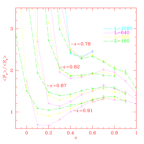
Figure 1: Ratio $\langle{P_{\epsilon}\rangle/\langle S_{\epsilon}\rangle}$ for various $\epsilon$ values versus $c$

Our results were obtained from a Monte Carlo (MC) investigation using an $O(3)$ version of the Swendsen-Wang cluster algorithm [13] and consist of a minimum of 20,000 lattice configurations used for taking measurements. For each value of $\epsilon$ we studied $L=160$, 320 and 640 (for $\epsilon=.78$ we also studied $L=1280$).

In Fig.1 we show the numerical value of the ratio $r$ as function of $c$ for $\beta=0$ for four values of $\epsilon$ for the c.a. model on a T lattice. Three distinct regimes are manifest for each of the four values of $\epsilon$ investigated:

• For small $c$, $r$ is increasing with $L$, presumably diverging to $\infty$ (region 1).

• For intermediate $c$, $r$ is decreasing with $L$, presumably converging to 0 (region 2).

• For $c$ sufficiently large depending upon $\epsilon$, $r$ shows a very mild dependence upon $L$.

This can only mean that for these values of $\epsilon$ for small $c$ $P_{\epsilon}$ percolates, for intermediate $c$ $S_{\epsilon}$ percolates and for sufficiently large $c$ both $P_{\epsilon}$ and $S_{\epsilon}$ form rings with quite similar (possibly equal) values of $\eta$. Our data allow to deduce a semiquantitative ‘phase diagram’ in the $(c,\epsilon)$-plane of the percolation problem induced by the c.a. model on the T lattice for $\beta=0$.

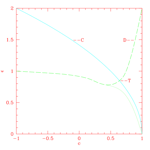
Figure 2: Phase diagram of the $O(3)$ model on the T lattice

This is shown in Fig.2. The solid line C is the curve $c=1-\epsilon^{2}/2$; above that line the two polar caps cannot touch and therefore their union cannot percolate. The dashed line D represents the minimal equatorial width above which $S_{\epsilon}$ percolates. The point T at the intersection of the curves D and C gives an upper bound for $c_{crt}$, the value of $c$ above which the c.a. model is massless.

Let us explain how this picture was obtained: since for $c=-1$ (no constraint) the model reduces to independent site percolation, for which the percolation threshold is known rigorously to be $\epsilon=1$, curve D has to start at $\epsilon=1$. With increasing $c$ that threshold shifts to smaller values of $\epsilon$. Four points of the dashed line are in fact determined by the data displayed in Fig.1: the clearly identifiable four points where the lines for different lattice sizes $L$ cross and the ratio $r$ becomes independent of $L$ determine the percolation threshold for the chosen value of $\epsilon$ and so determine a point of the dashed line D.

Two features of this diagram are worth emphasizing:
1. An equatorial strip of width less than approximately $\epsilon=.76$ never percolates.
2. In Fig.1 for approximately $c>0.4$ a range of $\epsilon$’s appears such that the ratio $r$ again becomes approximately independent of $L$. This is signalling the appearance of a new ‘phase’ in which both $S_{\epsilon}$ and $P_{\epsilon}$ form rings (the dotted line separates it from the region of percolation of $P_{\epsilon}$).

This regime of ring formation of both $S_{\epsilon}$ and $P_{\epsilon}$ is lying between the dotted and the dashed lines in Fig.2. Our data give strong evidence of its existence, but they do not determine in detail where the boundaries are. The dotted line has to run to $\epsilon=0$ for $c=1$ because below it there is percolation of $P_{\epsilon}$, and this is not possible above the solid line C $\epsilon=\epsilon_{c}$ (because it would conflict with the principle of non-coexistence of disjoint percolating sets). We drew the dashed line into upper right corner because we expect that eventually, for $c$ approaching 1, any polar cap will start forming rings, thereby preventing percolation of the corresponding equatorial strips.

But what it is essential for our conclusion that there is a massless phase is only that there is a regime below the dashed line D and above the solid line C, in which $S_{\epsilon}$ does not percolate and the two polar caps do not touch. In other words, the lines C and D have to cross (the crossing point is denoted by T in Fig.2). Since we found that for $\epsilon<\epsilon_{0}=0.76$ ${\cal S}_{\epsilon}$ never percolates, this means that for $c\geq c_{\epsilon_{0}}=0.71$ the model is massless. In fact the massless phase must start earlier, and for instance based on our data we estimate that at c=0.61 the c.a. model is already massless.

In the next section we will further corroborate the fact that for $\epsilon<0.76$ the equatorial strip does not percolate for any $c$.

We would like to comment briefly on another recent paper dealing with percolation properties of equatorial strips in the $O(3)$ model: Allès et al [14] published a study showing that for $\epsilon=1.05$ and $\beta=2.0$ in the s.a. model $S_{\epsilon}$ percolates. Although strictly speaking our percolation argument applies only to the c.a. model, the result of Allès et al is not surprising since at $\beta=2.0$ the s.a. model is clearly in its massive phase [15], hence, by analogy with what happens in the c.a. model, one would expect that clusters of a sufficiently wide equatorial strip percolate (see [16]). The real issue, which the authors of [14] did not seem to appreciate, is whether in the c.a. model clusters of the equatorial strip $S_{\epsilon_{c}}$ continue to percolate for $c$ sufficiently close to 1. The numerics presented in Fig.1 suggest that that is not the case.

4 Corroborating numerics

To corroborate our most important result, namely that for approximately $\epsilon<.76$ $S_{\epsilon}$ does not percolate for any value of $c$, we also measured (at $\beta=0$) the ratio of the mean cluster size of the set $P^{+}_{\epsilon^{\prime}}$ with $\epsilon^{\prime}=.5$ to that of the set $S_{\epsilon}$ with $\epsilon=0.75$ ($\epsilon^{\prime}$ was chosen so that $P^{+}_{\epsilon^{\prime}}$ has equal density with $S_{\epsilon}$). The results are shown in (Fig.3). This figure shows that for $c$ less than about 0.4 (and greater than 0) the ratio grows very rapidly with $L$, indicating that $P^{+}_{\epsilon^{\prime}}$ forms rings while $S_{\epsilon}$ has finite mean size; this region terminates around $c=0.4$, where presumably also $S_{\epsilon}$ starts forming rings, and the dependence of the ratio upon $L$ becomes much milder. Since for $c>0.4$ the ratio continues to grow with $L$, at equal density, clusters of the polar cap are larger than those of the equatorial strip. The larger average cluster size of the polar cap compared to the strip of the same area is probably due to the fact that the strip has a larger boundary than the polar cap. This is in agreement with a general conjecture stated in [8], namely that for $c$ sufficiently large, if two sets have equal area but different perimeters, the one with the smaller perimeter will eventually, for $c$ approaching 1, have larger average cluster size. For the case at hand, this is apparently true for all values of $c$.

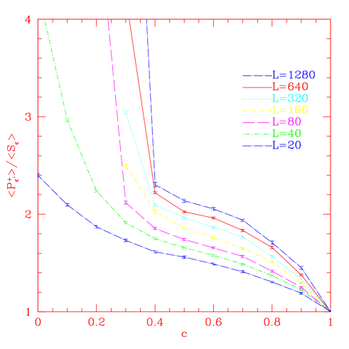
Figure 3: The ratio of the mean cluster size of a polar cap of height .75 to that of an equatorial strip of the same height

5 Comparison to the $O(2)$ model

The general belief, which we criticized in ref.[4], is that there is a fundamental difference between abelian and nonabelian models. To test this belief we also studied the ratio $r$ for the c.a. $O(2)$ model on the T lattice. The phase diagram is shown in Fig.4. Since in the $O(2)$ model the set ${\cal P}_{\epsilon}$ can also be regarded as a set ${\cal S}_{\tilde{\epsilon}}$ where $\tilde{\epsilon}=\sqrt{4-\epsilon^{2}}$, certain features of that diagram follow from rigorous arguments. For instance it is clear that in the c.a. model there exist two intersecting curves C and $\tilde{\rm C}$ and in the region to their right the model must be massless [6, 7]. The precise location of the curves $D$ (or $\tilde{D}$) must be determined numerically, something which we did not do. We did verify though that the ring formation region begins around $c=-0.5$.

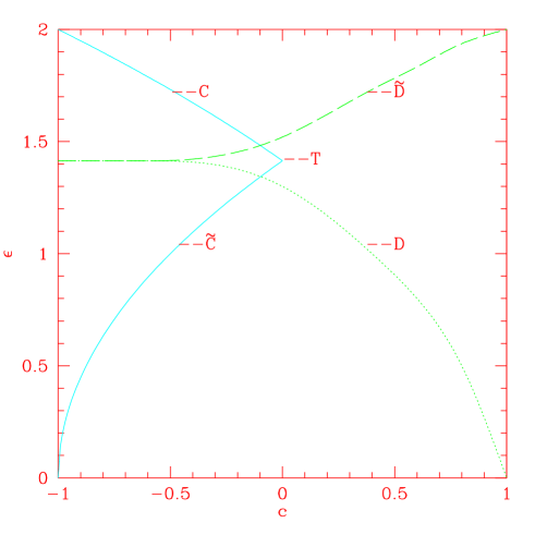
Figure 4: The phase diagram for the $O(2)$ model on the T lattice

6 Universality between the s.a. and c.a. models

In our opinion the arguments and numerical evidence provided so far give strong indications that the c.a. $O(3)$ model on the T lattice has a massless phase. Universality would suggest that a similar situation must exist for the s.a. models on the T and S lattices. To test universality we measured on the S lattice the renormalized coupling both on thermodynamic lattices in the massive phase and in finite volume in the presumed critical regime (as in [17]). Our data for the c.a. model on the S lattice only determine an interval (about $.5$ to $.7$) in which the massless phase of the model sets in; we tried to see if we could get a similar $L$ dependence for the renormalized coupling in the s.a. model at a suitable $\beta$ as for $c=.61$ in the c.a. model at $\beta=0$. This seems to be indeed the case for $\beta$ roughly $3.4$. We went only up to $L=640$, hence this equivalence between $c$ and $\beta$ should be considered only as a rough approximation, but there seems to be no doubt that the two models have the same continuum limit.

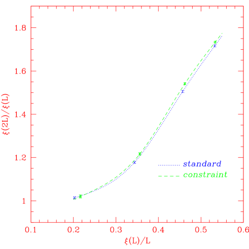
Figure 5: The step scaling curves of the s.a. and c.a. $O(3)$ models on the T lattice

We also compared the step scaling curve in the s.a. and c.a. models. The step scaling curve is obtained as follows: on a periodic lattice of size $L\times L$ we define an apparent correlation length $\xi(L)$. Namely let $P=(p,0)$, $p={2n\pi\over L}$, $n=0,1,2,...,L-1$. Then define

$$\xi(L)={\sqrt{3}\over 4\sin(\pi/L)}\sqrt{G(0)/G(1)-1}$$ (5)

where

$$G(p)={1\over L^{2}}\langle|\hat{s}(P)|^{2}\rangle;\ \ \hat{s}(P)=\sum_{x}e^{iPx}s(x)$$ (6)

Leaving $\beta$ respectively $c$ fixed, one doubles $L$ and measures also $\xi(2L)$. The step scaling function gives the ratio $2\xi(L)/\xi(2L)$ versus $L/\xi(L)$. In the continuum limit ($L\to\infty$ and $\beta\to\beta_{\it crt}$ at $L/\xi(L)$ fixed), this procedure produces a unique curve characterizing the universality class of the model. In Fig.5 we present the step scaling function for the c.a. and s.a. models. The data were produced by adjusting $\beta$ and $c$ so that at $L=20$ we obtain roughly the same $\xi(L)$ in the two models. After that, leaving $\beta$ respectively $c$ fixed, $L$ was doubled until $L=320$. As can be seen, the two step scaling curves agree reasonably well; the slight disagreement is probably due to the fact that the two curves have to agree only in the continuum limit ($\xi\to\infty$), i.e. they have different lattice artefacts, whereas the largest value of $\xi$ reached was only approximately 35 lattice units.

7 Heuristic explanation of the transition

It is intersting to note that there is a heuristic explanation for both the existence of a massless phase in the s.a. $O(3)$ model and for the value of $\beta_{\it crt}$. Indeed it is known rigorously that in $2D$ a continuous symmetry cannot be broken at any finite $\beta$. In a previuos paper [5] we showed that the dominant configurations at large $\beta$ are not instantons but superinstantons (s.i.). In principle both instantons and s.i. could enforce the $O(3)$ symmetry. In a box of diameter $R$ the former have a minimal energy $E_{\it inst}=4\pi$ [18] while the latter $E_{s.i.}=\delta^{2}\pi/\ln R$, where $\delta$ is the angle by which the spin has rotated over the distance $R$. Now suppose that $\beta_{\it crt}$ is sufficiently large for classical configurations to be dominant. Then let us choose $\delta=2\pi$ (restoration of symmetry) and ask how large must $R$ be so that the superinstanton configuration has the same energy as one instanton. One finds $\ln R=\pi^{2}$. But in the Gaussian approximation

$$\langle s(0)\cdot s(x)\rangle\approx 1-{1\over\beta\pi}\ln x$$ (7)

Thus restoration of symmetry occurs for $\ln x\approx\pi\beta$. This simpleminded argument suggests that for $\beta\geq\pi$ instantons become less important than s.i.. Now in a gas of s.i. the image of any small patch of the sphere forms rings, hence the system is massless. While this is not a quantitative argument, we believe it captures qualitatively what happens: a transition from localized defects (instantons) to super-instantons.

8 Absence of asymptotic freedom

Next let us discuss the connection between a finite $\beta_{crt}$ and the absence of asymptotic freedom. It follows from our earlier work concerning the conformal properties of the critical $O(2)$ model [10]. We refer the reader for details to that paper and give only an outline of the argument. The s.a. lattice $O(N)$ model possesses a conserved isospin current. This currrent can be decomposed into a transverse and longitudinal part. Let $F^{T}(p)$ and $F^{L}(p)$ denote the thermodynamic values of the 2-point functions of the transverse and longitudinal parts at momentum $p$, respectively. Using reflection positivity and a Ward identity we proved that in the massive continuum limit the following inequalities must hold for any $p\neq 0$:

$$0\leq F^{T}(p)\leq F^{T}(0)=F^{L}(0)\leq F^{L}(p)=2\beta E/N$$ (8)

Here $E$ is the expectation value of the energy

$$E=\langle s(i)\cdot s(j)\rangle$$

at inverse temperature $\beta$. Since $E\leq 1$ it follws that if $\beta_{\it crt}<\infty$ $F^{T}(0)-F^{T}(p)$ cannot diverge for $p\to\infty$ as required by perturbative asymptotic freedom [19]. In fact, for $\beta_{crt}=3.4$ (which is a reasonable guess) $F^{T}(p)$ must be less than 2.27, in violation of the form factor computation giving $F^{T}(0)-F^{T}(\infty)>3.651$ [20].

9 Concluding remarks

Since the implications of our result, that for the c.a. model a sufficiently narrow equatorial strip never percolates, are so dramatic, the reader may wonder how credible are the numerics. The only debatable point is whether our results represent the true thermodynamic behaviour for $L\to\infty$ or are merely small volume artefacts. While we cannot rule out rigorously the latter possibility, certain features of the data make it highly implausible:

• Small volume effects should set in gradually, while the data in Fig.1 indicate a rather abrupt change from a region where $r$ is decreasing with $L$ to one where $r$ is essentially independent of $L$.

• For $c\to 1$ at fixed $L$, $r$ must approach the ‘geometric’ value $r=2/\epsilon-1$. As can be seen, in all the cases studied, throughout the ‘ring’ region $r$ is clearly larger than this value, while it should go to 0 if $S_{\epsilon}$ percolated.

• In Fig.3 there is no indication of the ratio going to 0 for increasing $L$. Moreover the dramatic change in slope around $c=.4$ indicates that the polar cap $P_{\epsilon^{\prime}}$ starts forming rings at a smaller value of $c$ than the equatorial strip $S_{\epsilon}$.

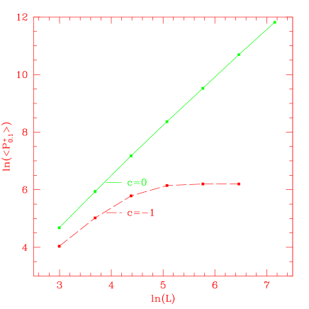
Figure 6: Mean size of clusters of the polar cap $P^{+}_{0}.1$ at $c=-1$ (Bernoulli) and at $c=0$ versus $L$. The correlation length $\xi$ is approximately 53 lattice units.

We have additional numerical evidence that clusters of a polar cap $P^{+}_{\epsilon}$ smaller than a hemisphere ($s\cdot n>\epsilon/2>0$) form rings for some $c<1$. Namely we investigated the case $\epsilon=0.1$. For the the case $c=-1$ (Bernoulli percolation) it is known rigorously that clusters of this set have finite mean size. As can be seen from Fig.6 our numerical values at $c=-1$ corroborate this fact. In the same figure we show the mean cluster size of cluster of $P^{+}_{0.1}$ at $c=0$, where the correlation length is approximately 53 lattice units. Even though we increased $L$ up to 1280, the mean cluster size shows no sign of leveling off, growing in fact like some power of $L$, consistent with the formation of rings.

Therefore there is good numerical evidence that for $c=0$, where we can reach the thermodynamic limit, clusters of this polar cap form rings. The natural expectation would be that the mean cluster size of a subset of a hemisphere is a nondecreasing function of $c$. This is borne out by the numerics, as shown in Fig.7. There we represent the mean cluster size of $P^{+}_{0.1}$ at fixed $L=640$ function of $c$. The data support the assertion that for any $c>0$ the mean size of the clusters of $P^{+}_{0.1}$ diverges, which, via our argument, implies that the c.a. model must cease being massive for some $c<1$.

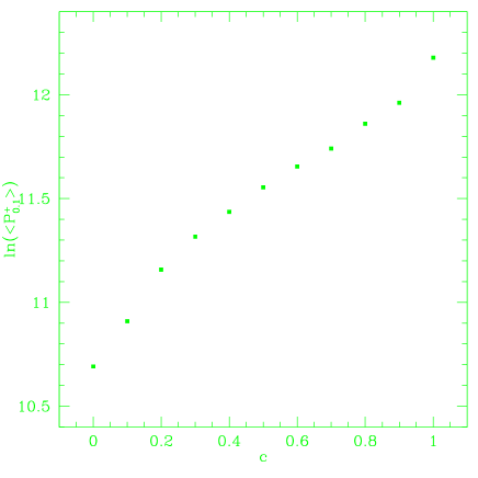
Figure 7: Mean size of clusters of the polar cap $P^{+}_{0}.1$ at $L=640$ versus $c$.

Thus we doubt very much that the effects we are seeing represent small volume artefacts. Moreover, if $s_{z}$, the $z$-component of the spin $s$ remained massive at low temperature and in fact an arbitrarily narrow equatorial strip percolated, one would have to explain away our old paradox [8, 9]: if such a narrow strip percolated, an even larger strip would percolate and on it one would have an induced $O(2)$ model in its massless phase, in contradiction to the Mermin-Wagner theorem.

Consequently it seems unavoidable to conclude that the phase diagram in Fig.2 represents the truth, that a soft phase exists both in the s.a. and the c.a. model and that the massive continuum limit of the $O(3)$ model is not asymptotically free. In a previous paper [5] we have already shown that in nonabelian models even at short distances perturbation theory produces ambiguous answers. The present result sharpens that result by eliminating the possibility of asymptotic freedom in the massive continuum limit.

Acknowledgement: AP is grateful to the Humboldt Foundation for a Senior US Scientist Award and to the Werner-Heisenberg-Institut for its hospitality.

References

- [1] J. Fröhlich and T. Spencer, Comm. Math. Phys. 83 (1982) 411.
- [2] Open Problems in Mathematical Physics, http://www.iamp.org
- [3] A. Patrascioiu, Phys.Rev.Lett. 58 (1987) 2285.
- [4] A. Patrascioiu and E. Seiler, Difference between abelian and nonabelian models: Fact and Fancy, MPI preprint 1991, math-ph/9903038.
- [5] A. Patrascioiu and E. Seiler, Phys.Rev.Lett. 74 (1995) 1920.
- [6] A. Patrascioiu and E. Seiler, Phys. Rev. Lett. 68 (1992) 1395, J. Stat. Phys. 69 (1992) 573.
- [7] M. Aizenman , J. Stat. Phys. 77 (1994) 351.
- [8] A. Patrascioiu, Existence of algebraic decay in non-abelian ferromagnets preprint AZPH-TH/91-49, math-ph/0002028.
- [9] A. Patrascioiu and E. Seiler, Nucl.Phys.(Proc.Suppl.) B30 (1993) 184.
- [10] A. Patrascioiu and E. Seiler, Phys.Rev. E57 (1998) 111, Phys.Lett. B417 (1998) 123.
- [11] L. Russo, Z. Wahrsch. verw. Gebiete, 43 (1978) 39.
- [12] P. W. Kasteleyn and C. M. Fortuin, J. Phys. Soc. Jpn. 26 (Suppl.) (1969) 11; C. M. Fortuin and P. W. Kasteleyn, Physica 57 (1972) 536.
- [13] Robert H. Swendsen and Jian-Sheng Wang, Phys. Rev. Lett. 58 (1987) 86.
- [14] B. Allès, J. J. Alonso, C. Criado and M. Pepe, Phys.Rev.Lett. 83 (1999) 3669.
- [15] J. Apostolakis, C. F. Baillie and G. C. Fox, Phys.Re. D43 (1991) 2687.
- [16] A. Patrascioiu and E. Seiler, Phys.Rev.Lett 84 (2000) 5916.
- [17] J.-K. Kim and A. Patrascioiu, Phys.Rev. D47 (1993) 2588.
- [18] A. A. Belavin and A. M. Polyakov, JETP Letters 22 (1975) 245.
- [19] J. Balog, Phys. Lett. B 300 (1993) 145.
- [20] J. Balog and M. Niedermaier, Nucl.Phys. B500 (1997) 421.