Discrete Lorentzian Quantum Gravity
Abstract
Just as for non-abelian gauge theories at strong coupling, discrete lattice methods are a natural tool in the study of non-perturbative quantum gravity. They have to reflect the fact that the geometric degrees of freedom are dynamical, and that therefore also the lattice theory must be formulated in a background-independent way. After summarizing the status quo of discrete covariant lattice models for four-dimensional quantum gravity, I describe a new class of discrete gravity models whose starting point is a path integral over Lorentzian (rather than Euclidean) space-time geometries. A number of interesting and unexpected results that have been obtained for these dynamically triangulated models in two and three dimensions make discrete Lorentzian gravity a promising candidate for a non-trivial theory of quantum gravity.
1 QUANTUM GRAVITY
For the purposes of this presentation, quantum gravity will be defined as the non-perturbative quantization of the classical theory of general relativity, with and without the inclusion of other matter fields and interactions. Judging from our current knowledge of the fundamental laws of physics, it seems highly likely that at sufficiently large energies also gravitational interactions should be governed by quantum rather than by classical equations of motion. Quantum gravity – whose theoretical formulation is still elusive – should include a consistent description of local quantum phenomena in the presence of strong gravitational fields.
It has been known for a long time that perturbative quantum gravity, based on a decomposition
| (1) |
of the Lorentzian space-time metric into the flat Minkowski metric and a linear perturbation (representing the degrees of freedom of a massless spin-2 graviton), leads to a non-renormalizable field theory. Although this does not preclude the use of the perturbation series as an effective description of quantum gravity in the presence of an energy cut-off, it cannot serve as the definition of a fundamental theory.
The ensuing need to quantize gravity non-perturbatively is not confined to field theory, but persists in string-theoretic formulations (where it is an unsolved problem as well). Imagine trying to obtain a quantum state representing a 4d Schwarzschild black hole with metric
| (2) |
by superposing gravitonic excitations within string theory. However, because of the proportionality for Newton’s constant [1], this involves arbitrary powers of the string coupling , and is therefore an intrinsically non-perturbative construction.
1.1 How do we quantize gravity non-perturbatively?
The great success of lattice models in describing non-perturbative properties of QCD has for a long time been a motivation for applying discrete methods also in quantum gravity. I will be reporting on the status quo of path-integral (“covariant”) lattice models for quantum gravity, and on how to make them more Lorentzian. However, it should be pointed out that there are other ways of tackling the problem, most notably, in a canonical continuum approach based on a gauge-theoretic formulation of gravity in four dimensions [2].
Non-perturbative formulations of gravity usually involve suitable versions of the space of all 4d space-time geometries (of space-time metrics modulo diffeomorphisms), and all lattice models start from a discretized version of this classical configuration space. Note that giving up the notion of a preferred flat background metric also means that the Poincaré group will not appear as a fundamental symmetry group of the base space . This has nothing to do with the loss of the smooth manifold structure during discretization, but is a typical feature of all non-perturbative, background-independent formulations.
Among the important (and difficult) questions one may ask in discrete
quantum gravity are the following:
(i) how do we construct quantum gravity lattice models
that are well-defined, convergent statistical systems
at finite volume? How is the absence of a preferred background metric
reflected in the lattice construction?
(ii) Do these models lead to
interesting continuum theories in the infinite-volume limit? What
are their physical excitations?
(iii) What is the (quantum) geometry of the ground state of the
theory? Do we recover semi-classical geometries in a suitable limit?
1.2 Where do we stand?
The three most popular approaches to discrete quantum gravity in four
dimensions are:
Covariant Gauge Approaches, based on gauge-theoretic
first-order formulations of gravity with connections and vierbeins
(mostly on regular cubic lattices); they were studied intensely
for about ten years, starting in the late 70s [3]. More recently,
discrete gauge-theoretic formulations have seen a revival in the
context of so-called spin foam models for gravity, based on ideas
coming from topological quantum field theory [4].
Quantum Regge calculus is based on the
second-order form of gravity in terms of metric fields.
Space-time is approximated by
a simplicial complex, and the sum over all geometries takes the
form of a sum over all possible lengths of the edges of this complex.
This approach to quantum gravity originated in the mid-80s and is
still being pursued [5].
The method of Dynamical Triangulations is
a more recent variant of the quantum Regge calculus
program, where all edge lengths are frozen in, and the state sum is
taken over all possible manifold-gluings of a set of
equilateral simplicial building blocks. Although this is the most
recent of the three approaches
(started in the early 90s [6, 7]), the
number of research papers written in this area is by far the largest.
Interest in this formulation was largely propelled by its success in
reproducing results from continuum Liouville gravity in
. –
I will not dwell on a detailed description of the individual
achievements of these approaches, since this has been done both
in previous overview talks at lattice conferences, and in a recent
review article on the subject [8].
What has been learned from these investigations? Maybe not surprisingly, analytic results in 4d have proved hard to come by, although qualitative estimates of the partition function in certain phases can sometimes be made. Efficient numerical methods for models of fluctuating geometry and/or lattices have been developped and refined. The phase structures of all of the models described above have been investigated and their phases characterized in geometric terms, showing some surprising similarities across the various formulations [8]. However, it is probably fair to say that in spite of occasional claims to the contrary, there is so far no convincing evidence of a second-order phase transition in these models, which is usually taken as a necessary condition for the existence of an underlying continuum theory with propagating field degrees of freedom.
1.3 What to do?
Various strategies have been tried to improve on this somewhat unsatisfactory state of affairs, usually by modifying the measure of the quantum theory, or by adding appropriate matter fields. I refer to last year’s review talk by Krzywicki [9] for a more detailed account of these attempts. The most recent development in this area concerns the addition of non-compact U(1)-gauge fields in the dynamical triangulations approach. The phase structure of these models does indeed appear changed with respect to the pure-gravity models [10], but more recently it has been understood that this is a “spurious” effect, and completely equivalent to a rescaling of the measure by factors of the determinant of the metric [11]. Conflicting numerical results on this issue have been reported at this conference [12], so this may still hold out some hope for more interesting findings in this matter-coupled model. However, the general consensus seems to be that more radical changes of the discrete models are required to alter these negative results.
1.4 Absence of a Wick rotation
Unfortunately, until recently it seemed that we had run out of natural, geometrically motivated ways of modifying the discrete gravity models. There is another reason for why the situation may be yet more serious: even if some of these quantization attempts had been successful, their connection with the physical, Lorentzian theory of quantum gravity would have remained unclear, because they all work with configuration spaces of (positive-definite) Euclidean geometries. There are of course good technical reasons for making the substitution
| (3) |
since state sums over complex phase factors usually diverge. Well-motivated though it may be, it should be pointed out that in a non-perturbative context, (3) is an ad hoc substitution. Although (3) may look suggestive, unlike in ordinary field theory on a Minkowski background, there is no a priori concept of a “Wick rotation” in a theory with a dynamical metric. The problem lies in the fact that we must Wick-rotate all metrics, but that almost all metrics (unless they have special symmetries, for example, time-like Killing vectors) have no geometrically distinguished notion of “time”. (Recall that in general relativity denotes simply “coordinate time”, and can be changed by a diffeomorphism without affecting physical results.) However, a prescription like is certainly not diffeomorphism-invariant (think of a simple coordinate transformation like , for ).
Since there is a certain reluctance to recognize this as a problem, let me add some further remarks on the issue. It does of course not follow from the discussion above that suitable Wick rotations do not exist. However, they should be constructed explicitly, and their naturalness and/or uniqueness be shown. Also, one might hope that once an interesting continuum limit of Euclidean quantum gravity is found, a continuation to Lorentzian signature might be obvious. This is a logical possibility, but it has not yet been realized.
At any rate, there is no a priori reason that a theory based on a non-perturbative path integral for Riemannian (or Euclidean) metrics should be related in any simple way to one based on Lorentzian metrics. Interpreted positively, this observation may offer us a way out of the current impasse in finding physically interesting quantum gravity models. Our failed attempts to quantize could be closely related to the fact that the Lorentzian nature of gravity is not appropriately taken into account. As I will describe in more detail below, there is now evidence from discrete Lorentzian models of gravity in two and three space-time dimensions supporting this point of view.
1.5 Going Lorentzian
In the continuum, a Lorentzian space-time is usually given in the form of a metric field tensor on some manifold , with signature (–+++), where is symmetric and non-degenerate, but not necessarily diagonal. The associated line element
| (4) |
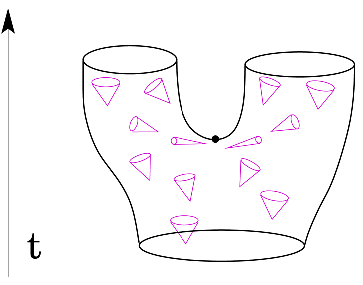
may therefore take values , or , depending on whether the infinitesimal distance measured on is time-like, light-like or space-like. It follows that the neighbourhood of any point has a light-cone structure, where the light-cone consists of all points that can be connected to by curves whose tangent vectors are everywhere light-like, with analogous prescriptions for points in- and outside the light-cone. Just as it does in Minkowski space, this implies a local causal structure: a point lies to the future (past) of , if there is a future- (past-)oriented curve from to that is nowhere space-like. Otherwise, and are not causally related. In addition, one usually requires a well-defined causal structure globally, to avoid pathologies such as closed time-like curves. Note also that branching points, associated with a topology change of spatial slices (Fig. 1) are not compatible with a well-defined Lorentzian structure, since the light-cones must necessarily degenerate at such points. – By contrast, in Euclidean metric spaces there is no distinction between space- and time-like directions.
How can Lorentzian features be built into a framework of discretized geometries? Regge’s prescription for approximating smooth geometries by piecewise linear spaces works just as well (and was originally conceived) for Lorentzian signature. The work described below may be regarded as a Lorentzian version of the dynamical triangulations (DT) approach to quantum gravity. We prefer this method over quantum Regge calculus, since we are interested in an analytic formulation (which even for is impossible in Regge calculus, due to the presence of triangle inequalities) and because the evidence from suggests that DT deals correctly with the diffeomorphism symmetry of the theory.
In a Lorentzian DT approach, one may expect to have both time- and space-like edges (and possibly even null-edges). However, a random assignment of squared edge lengths , say, to an arbitrary simplicial complex (a “triangulation”) will in general not lead to a metric structure of the correct signature and without closed time-like curves. Our strategy will be to first identify a large class of well-defined discrete causal triangulations (without restricting the local curvature degrees of freedom). In order to make the associated partition function convergent, we will then use a Wick rotation to map each discrete Lorentzian geometry into a unique Euclidean geometry. After the sum and the continuum limit have been performed, the propagator is “rotated back”. Our particular choice of the fundamental building blocks, described below, is motivated by a simple form for both the path integral and the Wick rotation.
2 THE NEW IDEA
Let me now turn to an explicit description of the Lorentzian DT model, which incorporates a notion of causality and possesses a “Wick rotation” [13, 14, 15]. The partition function takes the form of a sum over causal triangulations with certain edge length assignments,
| (5) |
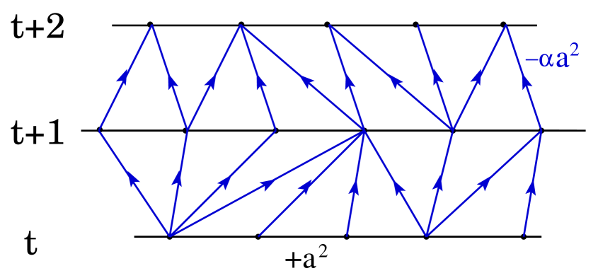
with each contribution weighted by the Regge action (the simplicial version of the -dimensional Einstein action, including a cosmological constant ) associated with and a discrete symmetry factor . The triangulations appearing in the sum (5) all have a foliated structure, where successive (d–1)-dimensional spatial slices (realized as equilateral Euclidean triangulations of squared edge length ) are connected by time-like, future-oriented edges of length-squared , with . This is most easily illustrated in 1+1 space-time dimensions (Fig. 2), where the spatial slices are simply given by chains of space-like edges. In addition, to reflect the causal properties of the continuum geometries these piece-wise linear spaces are supposed to approximate, we do not allow for any spatial topology changes. For simplicity, we use compactified and connected spatial slices, yielding a space-time topology .
As mentioned earlier, we can now define a unique Wick rotation on any discrete Lorentz geometry of this type by substituting all time-like links with by space-like links with squared edge length . One can show [14, 15] that this analytic continuation in has the desired effect of inducing
| (6) |
on the weights. It is important to realize that the set of Euclidean triangulations obtained after the Wick rotation is strictly smaller than the set of all Euclidean triangulations. It is precisely this feature that leads to a change of universality class of the Lorentzian models, compared with the Euclidean ones. One could rephrase this by saying that we have introduced a different measure, which however was not chosen ad hoc, but motivated by physical and geometric considerations. Obviously, in the end only the solution of this model and its physical properties can tell us whether this ansatz is justified. In this regard, we are encouraged by the results obtained so far in dimensions two and three.
What has been shown is that for finite lattice volume in and 4, the discrete Lorentzian models are completely well-defined, in the sense that the associated transfer matrices in the discrete propagators
| (7) |
(where g denotes a discrete spatial geometry) are bounded and strictly positive. The slice parameter has a natural physical interpretation as a discrete proper time, that is, the time experienced by an idealized set of observers freely falling along geodesics perpendicular to surfaces of constant . Our next task will be to understand the continuum theories associated with these models. Fortunately, at least in , Lorentzian quantum gravity turns out to be exactly soluble.
3 LORENTZIAN GRAVITY IN D=2
In two space-time dimensions, the Einstein action for a fixed topology reduces to the cosmological term
| (8) |
where is the number of triangles in the triangulation , and is the bare cosmological constant. The most natural propagator in Lorentzian gravity is a “two-loop function”, describing the transition amplitude between an initial geometry of length and a final geometry of length (with integer lengths ) in time steps. Its functional form after the Wick rotation (and setting ) becomes simply [13, 16]
| (9) | |||||
The last expression on the right makes it clear that solving the model is tantamount to solving the combinatorial problem of counting the number of inequivalent causal triangulations of volume and length , for given lengths and . (Similar statements hold in higher dimensions too.)
In two dimensions, this problem can be solved explicitly, and leads after continuum limit, renormalization and an inverse Wick transformation to the continuum amplitude
| (10) |
where is the Bessel function, and , and are the renormalized counterparts of the bare constant and of and . The theory described by (10) is unitary, and its Hamiltonian can be mapped onto a three-dimensional harmonic oscillator with spin and diagonalized explicitly [17]. Modified versions of 2d Lorentzian gravity (including a higher-order curvature term, and “decorations” by dimers and a restricted class of baby universes) have also been solved analytically [18], leading to similar results.
3.1 Geometry of the ground state in 2d
What is the physics described by this model? There cannot be much physics to speak of, since classical gravity in 2d is an empty theory. All one can expect are quantum fluctuations at the Planck scale (which happens to coincide with the cosmological scale, since the theory has only a single length scale). Nevertheless we can investigate the geometric properties of the ground state of the quantum theory and compare them with the Euclidean case.
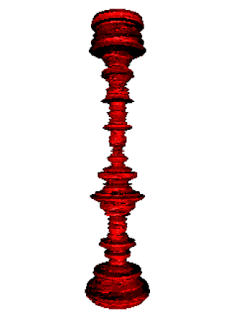
Fig. 3 shows a typical 2d Lorentzian space-time, taken from a Monte Carlo simulation. Observe how the size of the compactified spatial slices changes as a function of proper time (pointing upwards). These fluctuations are indeed large, and of the same order as the average spatial length, .
A rough way of characterizing the quantum geometry is through its Hausdorff dimension . It can be measured by finding the scaling behaviour of the volumes of geodesic balls of radius in the ensemble of Lorentzian geometries,
| (11) |
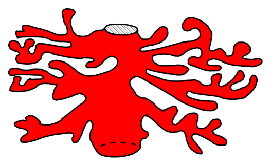
It is straightforward to extract from the propagator, yielding . This may not seem a surprising result, since we started from an ensemble of two-dimensional triangulations. However, it is by no means a foregone conclusion, since it is a property of the entire quantum ensemble (which, as we have seen, is subject to large fluctuations). Besides, we already know an example where this does not happen, namely, Euclidean (or “Liouville”) quantum gravity in two dimensions, which has ! In this case, it is an indication of the highly fractal nature of the quantum geometry, which is completely dominated by so-called baby universes (Fig. 4).
Such highly branched configurations cannot occur in the Lorentzian state sum, since they are not compatible with our causality conditions. It can be shown explicitly that this is the central difference between the two formulations, causing them to lie in different universality classes. This observation has also been used to relate the two models by a renormalization procedure that amounts to an “integrating out of baby universes” [19]. It demonstrates that the relation between the two continuum theories is rather more complicated than a simple analytic continuation .
Thus we see that the physics described by the Lorentzian quantum gravity model is completely different from that of the Euclidean one. Obviously, since quantum gravity in two dimensions is an unphysical theory, there is not much to choose between the two theories; we cannot perform experiments to determine which of them is “correct”, nor is there any a priori preference for a particular metric signature. However, let us for the moment assume that we were interested in obtaining a theory of Lorentzian geometries (as arguably is the case in ). One could then argue that it was unnatural to single out a “time” in the purely Euclidean theory, since the fractal geometries have no distinguished directions anywhere. Although it is clearly possible to make an arbitrary choice of a time parameter, this will typically result in constant-time slices that are highly multiply connected and undergo constant topology changes. Again, this may not be of great concern in dimension 2, but if a similar behaviour was found in , one would have to make sure that it did not lead to consequences in contradiction with observations.
3.2 Coupling 2d Lorentzian gravity to matter
I will now briefly describe the properties of Lorentzian gravity coupled to matter fields. The partition function for the coupled model takes exactly the same form as in Euclidean DT, but again with the sum taken over causal triangulations only. For an Ising model with nearest-neighbour interaction it is given (in the Euclidean sector) by
| (12) |
where the last sum is over all possible spin configurations of the Ising model on the triangulation . We are interested both in the critical properties of the matter on this non-trivial “background” and in possible back reactions of the matter on the geometry, since the latter is represented by a fluctuating ensemble. Our main reference point for such a system is Euclidean Liouville gravity with an Ising model, where the critical matter exponents (specific heat, magnetization, magnetic susceptibility) are changed from their Onsager values on fixed, regular lattices (, , ) to , and [20].
The Lorentzian model has not yet been solved exactly, but we have performed both a high-temperature expansion and Monte Carlo simulations to determine its critical behaviour. (The diagrammatic expansion used in the former has some non-standard features, since the graph counting takes place in a fluctuating ensemble of geometries.) At the combined critical point of the cosmological coupling and the matter coupling , they consistently yield the Onsager exponents for the Ising matter [21]. This may be surprising at first, since one could have been tempted to interpret the outcome of the Euclidean system cited above as an indication that the critical matter behaviour must necessarily change in the presence of a fluctuating geometry. Here we have an example where this is not the case. Another lesson is that we also may not draw the converse conclusion, namely, that Onsager exponents for the matter necessarily imply that the underlying geometry is fixed and flat. On the contrary, we have to conclude that these exponents are rather “robust”, and that the geometry has to be very distorted in order to cause a change of the critical matter behaviour. (Note that one could try to turn this into a method for determining critical matter exponents: simply couple them to Lorentzian lattices. For the case of the Ising model, we found a remarkably good convergence of the diagrammatic expansion for the susceptibility [21].)
3.3 … and more matter
In 2d Lorentzian gravity coupled to a single model of Ising spins, we did not find any appreciable back reaction of the matter on the geometry (i.e. one that would have survived the continuum limit). However, as more matter is coupled to the system ( Ising models, with ), this is no longer true. The coupling is achieved by substituting the last sum in (12) by a sum over independent copies of the Ising model on the given triangulation . There is a very good reason for studying this situation. In the language of conformal systems, a system with Ising models at its critical point gives rise to a conformal field theory with central charge . However, Liouville-matter models with are known to be inconsistent, in the sense that their critical exponents become complex. (This also goes by the name of “ barrier” in bosonic string theory, where plays the role of embedding dimension.)
In the Lorentzian case, we have found no such inconsistencies. We have performed Monte Carlo simulations at [22], where the combined system seems perfectly well-defined, and – within the numerical error bars – the matter behaviour is again governed by the Onsager exponents! (The value 8 was chosen to be well beyond the region , since the experience from Euclidean dynamical triangulations tells us that the phase change right at may not be very pronounced in numerical simulations.) In contrast with the case , we now observe a strong back reaction on the geometry, which results in a different universal behaviour of the gravitational sector. The impact of the matter coupling is best illustrated visually. Fig. 5 shows the coupling to a single Ising model at and . As far as the geometry of the configuration is concerned, there are no dramatic changes compared with pure gravity (Fig. 3). However, after switching on eight Ising models, a typical configuration looks like Fig. 6. The effect of the matter is to “squeeze off” part of the space-time to an effectively one-dimensional region which will play no part in the continuum limit. All interesting physics takes place in the remaining, extended part. In this region of the geometry, we have measured the Hausdorff dimension of space-time to be [22]. It is a tempting but completely unproven conjecture that the phase transition in the geometry takes place exactly at .
We can understand the influence of the matter qualitatively, since the spin models have an energetic preference for short boundaries between spin clusters of a given orientation. In a theory where the geometry can fluctuate, spins will therefore have the tendency to squeeze off part of the space-time geometry. In the case of Euclidean Liouville gravity, whose geometries are very branched to start with, this apparently leads to a complete degeneracy of the geometry beyond the barrier. By contrast, the geometry of the Lorentzian 2d model remains well-defined.
4 LORENTZIAN GRAVITY IN D=3
Which of the characteristic features of the 2d Lorentzian model generalize to higher dimensions and how do they differ from their Euclidean counterparts? Our next stop on the way to the physically relevant case is in three dimensions. Apart from being a new statistical model of three-dimensional fluctuating geometries, this theory has some intrinsic interest. Although largely an unphysical theory, 3d quantum gravity is an extensively studied system [23]. It is often invoked as a model system for the full theory, since its classical equations resemble in many ways those of general relativity. There are of course no physical field degrees of freedom, and after getting rid of the diffeomorphisms, the theory has a finite-dimensional phase space. Although one has not yet been able to make full use of this observation in a configuration space path-integral formulation, it suggests that one may still be able to solve 3d gravitational models analytically.
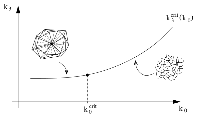
As mentioned earlier, we have constructed an extension of the simplicial Lorentzian formulation to 3 and 4 dimensions, on a set of causal and “Wick-rotatable” geometries. The model is finite and well-defined at finite volumes, without the need for further cut-offs [14, 15]. We have also shown that the extreme geometric phases found in Euclidean dynamical triangulations cannot be realized in the Lorentzian model. These phases of rather degenerate geometry make up the phase diagram of Euclidean DT in [24, 6], depicted in Fig. 8. At small inverse gravitational coupling one finds a “crumpled” phase, dominated by configurations of very large Hausdorff dimension (these are simplicial manifolds where roughly speaking any two vertices are a minimal distance apart). Above the first-order transition at , the system is in a branched-polymer phase of highly branched geometries (with a fractal dimension ). Unfortunately, neither of these phases seems to have a ground state that resembles an extended geometry of dimension .
The absence of these degenerate geometries from Lorentzian DT is an encouraging feature, but only a kinematic property, which does not necessarily prevent the occurrence of (less extreme) pathologies. To understand whether Lorentzian gravity does indeed solve some of the problems of the Euclidean approach, we need to investigate its phase structure by either numerical simulations or explicit analysis. This work is still in progress, and I will summarize our current understanding of the three-dimensional case. More technical details were reported by Ambjørn in the parallel session [25], and can also be found in [26]. In addition, efforts are under way to produce an analytical solution, by using matrix models methods [27] and a continuum treatment of the gravitational path integral in proper-time gauge [28].
4.1 Construction of 3d geometries
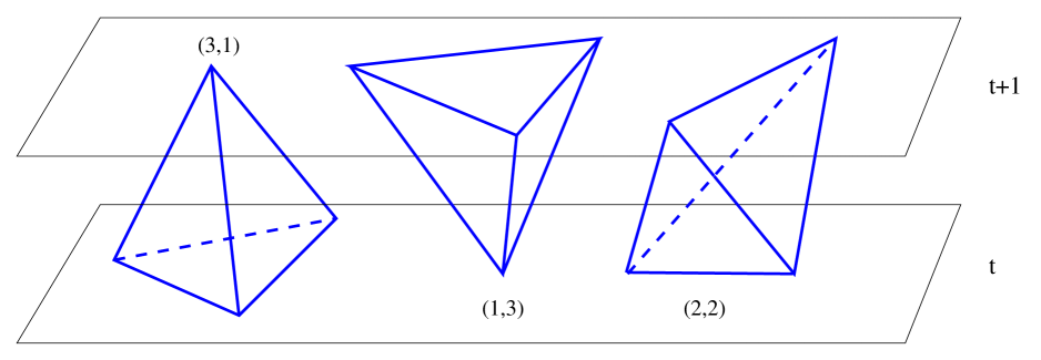
The 3d Lorentzian space-times have again a foliated structure, with spatial slices (of constant integer proper time ) given by equilateral Euclidean triangulations of the two-sphere. The space in between these slices is filled by three types of tetrahedral building blocks named (3,1), (1,3), and (2,2), according to the number of vertices they share with the spatial slices at times and +1 (Fig. 7). The analogue of the 1+1 dimensional strips in Fig. 2 are now 2+1 dimensional “sandwiches” . As in 2d, the spatial edges have squared lengths , and the time-like edges, interpolating between spatial slices, have . We can then compute Regge’s discretized action , , for a given Lorentzian simplicial manifold of this type. Since in the dynamical triangulations approach, both curvature (i.e. deficit angles) and volume come in discrete units, the action can be written as a function of two “bulk variables” (the numbers of d-dimensional simplices), and the total length of the geometry in proper time, leading to a partition function of the form
| (13) |
By a suitable analytic continuation in the complex -plane, one finds that the Lorentzian and Euclidean actions are (for , to satisfy Euclidean triangle inequalities) related by
| (14) |
For , the right-hand side takes the standard form familiar from Euclidean DT,
| (15) |
with the bare couplings ()
| (16) |
4.2 Phase structure of 3d Lorentzian gravity
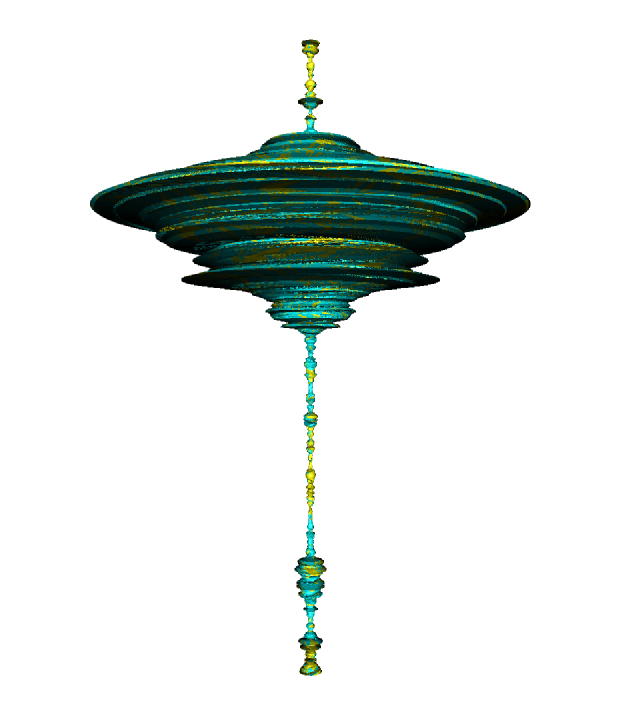
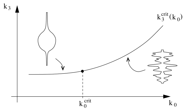
In order to study the 3d Lorentzian gravity path integral, we have set up a Monte Carlo simulation for the Wick-rotated system with partition function (13), at the Euclidean point . We have chosen as a convenient topology for our numerical purposes. The phase structure can be characterized as follows (Fig. 9). Just as in the Euclidean case, we find a first-order transition point along the critical line of the cosmological constant (along which a continuum limit exists). However, the geometry of the phases above and below this point are rather different. Above , the number of (2,2)-tetrahedra falls to a minimum, reducing the space-time to an uncorrelated ensemble of successive spatial slices, each well-described by Euclidean 2d gravity. This phase does not seem interesting from a physical point of view, because there are no long-range correlations in time-direction. A typical configuration from this “ragged” phase is shown in Fig. 11.
A similarly degenerate phase, where the numbers of (1,3)- and (3,1)-tetrahedra attain a minimum, may exist for small . Since our algorithm is not efficient in this region, we have not been able to explore whether there is a second (possibly negative) critical point . Wherever this second critical point may be, there is a remarkable structure that emerges in the region of intermediate coupling, , where all types of tetrahedra contribute non-trivially.


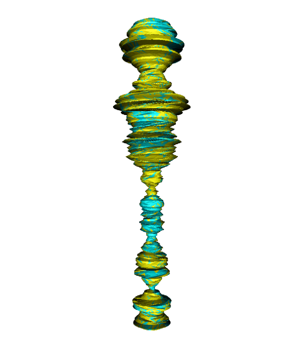
4.3 Geometry of the ground state in 3d
In this intermediate phase, we observe the emergence of an extended geometry of roughly spherical shape (Fig. 10 is a Monte Carlo “snapshot”), and a definite extension in -direction. This persists in the simulations at all volumes , provided the total length of the compactified time-direction is chosen sufficiently large, so that the “universe” can fit in. It is surprising (and unprecedented) that such a structure should emerge as the ground state of the quantum theory, given that we never put in any particular background geometry by hand. It is also rather straightforward to see that its presence cannot be explained as a minimum of the Euclidean action. It must therefore be the ground state of an effective action, where entropy contributions (in other words, the measure) play a crucial role. Apparently in our model these contributions are such that they outbalance potential conformal divergences coming from the Euclidean action (otherwise a well-defined ground state could not exist).
We have so far only investigated the macroscopic geometry of the universe, i.e. its scaling properties at “cosmic” scales [26]. These are compatible with the scaling of a three-dimensional object. Namely, the time extension scales according to , and the average two-volume of the spatial slices according to . A final question concerns the role of in this extended phase. The correlators between spatial volumes and certain distributions of spherical disc volumes within given spatial slices depend on , but we have found that they can be mapped onto each other by suitable (and equal) -dependent rescalings of the lengths of time- and space-like links. This leads us to conclude that the value of merely fixes an overall length scale, and otherwise does not affect the physics of the model.
5 SUMMARY
I have given a brief overview of the current status of covariant lattice approaches to four-dimensional quantum gravity. Activity in the area of Euclidean dynamical triangulations had somewhat slowed after a number of negative results concerning the nature of the phase transition (although it has by no means been shown that gravity cannot be quantized this way, if the current models are suitably modified). However, even if this approach leads eventually to a non-trivial continuum theory, some kind of “Wick rotation” will still be needed to make contact with physical geometries of Lorentzian signature and with physical observables.
A new class of Lorentzian dynamically triangulated models presents an alternative to these Euclidean approaches. Their starting point is a state sum over simplicial Lorentzian geometries, such that the Lorentzian nature of space-time is built in from the outset. All of them have a distinguished proper time, a well-defined causal structure, and can be uniquely Wick-rotated to Euclidean geometries. Topology changes of the spatial slices are not allowed.
From the point of view of statistical mechanics, they form a new class of models of random geometry (with a distinguished direction or “time arrow”). They are well-defined for finite space-time volumes, in the sense that their transfer matrices are bounded and strictly positive in dimension and 4, which implies the existence of a self-adjoint Hamiltonian with a spectrum that is bounded from below.
We have found that in two and three dimensions, the properties of the associated Lorentzian continuum theories are completely different from their Euclidean counterparts. It seems that the causality conditions imposed in the Lorentzian case act as an effective “regulator” on the geometry, still allowing for large local curvature fluctuations, but suppressing the fractal structures found in the Euclidean models in all dimensions. One consequence in two dimensions was that we could cross without problems the infamous barrier. In dimension three we observed, rather remarkably, the emergence of a ground state of extended three-dimensional geometry.
These results are very encouraging. Motivated entirely by physical considerations, we have discovered a new class of dynamically triangulated models for quantum gravity. In we have found a number of new and interesting results. We are particularly encouraged by the fact that the three-dimensional Lorentzian model has a phase with a ground state of extended and non-degenerate geometry, because this is exactly the point where the Euclidean DT model failed. The ultimate test is of course gravity in four space-time dimensions, where we expect a completely different picture, with propagating field degrees of freedom coming to the fore. It remains to be seen whether discrete Lorentzian quantum gravity can bring us any closer to this holy grail …
Acknowledgement. I thank J. Ambjørn, K.N. Anagnostopoulos and J. Jurkiewicz for enjoyable collaborations and A. Dasgupta and D. Marolf for (equally enjoyable) discussions.
References
- [1] J. Polchinski, String Theory II, Cambridge UP (1998), ch.14.
- [2] C. Rovelli, Living Rev. Rel. 1 (1998) 1; T. Thiemann, Living Rev. Rel., to appear.
- [3] L. Smolin, Nucl. Phys. B 148 (1979) 333; S. Caracciolo and A. Pelissetto, Nucl. Phys. B 299 (1988) 693.
- [4] J.C. Baez, in: Geometry and quantum physics, ed. H. Gausterer, Springer (2000).
- [5] M. Roček and R. Williams, Phys. Lett. B 104 (1981) 31; H. Hamber, Phys. Rev. D 61 (2000) 124008.
- [6] J. Ambjørn and J. Jurkiewicz, Phys. Lett. B 278 (1992) 42.
- [7] M.E. Agishtein and A.A. Migdal, Mod. Phys. Lett. A 7 (1992) 1039.
- [8] R. Loll, Living Rev. Rel. 1 (1998) 13.
- [9] A. Krzywicki, Nucl. Phys. Proc. Suppl. 83 (2000) 126.
- [10] S. Bilke et al, Phys. Lett. B 418 (1998) 226; 432 (1998) 279.
- [11] J. Ambjørn, K.N. Anagnostopoulos and J. Jurkiewicz, JHEP 9908 (1999) 016.
- [12] H.S. Egawa et al, hep-lat/0004021, 0010050.
- [13] J. Ambjørn and R. Loll, Nucl. Phys. B 536 (1998) 407.
- [14] J. Ambjørn, J. Jurkiewicz and R. Loll, Phys. Rev. Lett. 85 (2000) 924.
- [15] J. Ambjørn, J. Jurkiewicz and R. Loll, to appear.
- [16] J. Ambjørn, R. Loll, J.L. Nielsen and J. Rolf, Chaos Solitons Fractals 10 (1999) 177.
- [17] B. Dittrich, D. Kappel and R. Loll, to appear.
- [18] P. Di Francesco, E. Guitter and C. Kristjansen, Nucl. Phys. B 567 (2000) 515; hep-th/0010259.
- [19] J. Ambjørn, J. Correia, C. Kristjansen and R. Loll, Phys. Lett. B 475 (2000) 24.
- [20] D.V. Boulatov and V.A. Kazakov, Phys. Lett. B186 (1987) 379.
- [21] J. Ambjørn, K.N. Anagnostopoulos and R. Loll, Phys. Rev. D 60 (1999) 104035.
- [22] J. Ambjørn, K.N. Anagnostopoulos and R. Loll, Phys. Rev. D 61 (2000) 044010.
- [23] R. Loll, J. Math. Phys. 36 (1995) 6494; S. Carlip, Quantum Gravity in 2+1 Dimensions, Cambridge UP (1998).
- [24] J. Ambjørn, D.V. Boulatov, A. Krzywicki and S. Varsted, Phys. Lett. B 276 (1992) 432.
- [25] J. Ambjørn, J. Jurkiewicz and R. Loll, hep-lat/0011055.
- [26] J. Ambjørn, J. Jurkiewicz and R. Loll, to appear.
- [27] J. Ambjørn et al, to appear.
- [28] A. Dasgupta and R. Loll, to appear.