November 2000

KEK-TH-727

SACLAY-SPHT/T00/165

hep-th/0011175

Gaussian and Mean Field Approximations
for Reduced Yang-Mills Integrals

Satsuki Oda and Fumihiko Sugino
${}^{\ref{Oda}}$Institute of Particle and Nuclear Studies,
High Energy Accelerator Research Organization (KEK),
Tsukuba, Ibaraki 305-0801, Japan

${}^{\ref{Sugino}}$Service de Physique Théorique, C.E.A. Saclay,
F-91191 Gif-sur-Yvette Cedex, France

Abstract

In this paper, we consider bosonic reduced Yang-Mills integrals by using some approximation schemes, which are a kind of mean field approximation called Gaussian approximation and its improved version. We calculate the free energy and the expectation values of various operators including Polyakov loop and Wilson loop. Our results nicely match to the exact and the numerical results obtained before. Quite good scaling behaviors of the Polyakov loop and of the Wilson loop can be seen under the ’t Hooft like large $N$ limit for the case of the loop length smaller. Then, simple analytic expressions for the loops are obtained. Furthermore, we compute the Polyakov loop and the Wilson loop for the case of the loop length sufficiently large, where with respect to the Polyakov loop there seems to be no known results in appropriate literatures even in numerical calculations. The result of the Wilson loop exhibits a strong resemblance to the result simulated for a few smaller values of $N$ in the supersymmetric case.

1 Introduction

One of the most exciting topics about nonperturbative aspects of superstring theory or M-theory is their various connections to gauge theories. Matrix theory, whose classical action is given by that of one-dimensional Yang-Mills theory with maximal supersymmetry, has been conjectured as a nonperturbative definition of M-theory by Banks, Fischler, Shenker and Susskind (BFSS) [1]. Also, via its toroidal compactification on a circle and on a two-torus in the procedure of Taylor [2], it leads to a proposal for a nonperturbative definition of type IIA superstring theory [3, 4] and type IIB superstring theory [4, 5], respectively. They are given by two- and three-dimensional maximally supersymmetric Yang-Mills (SYM) theories. In addition, another definition of type IIB superstring theory, which takes the form of the above supersymmetric Yang-Mills theory completely reduced to a point, has been proposed by Ishibashi, Kawai, Kitazawa and Tsuchiya (IKKT) [6].

However, in order to definitely extract nonperturbative aspects of string theory from these matrix string models, we need to know also about those of SYM theories. In general, it still remains to be an extremely difficult problem, so until now the analysis has been done in the limited cases. In energy sufficiently higher than the string scale, there exists the region such that physics can be well described by a perturbative expansion around the specific instanton configuration of the SYM theory which describes the world sheet geometry in the string scattering process [8]. In the case of the IIA matrix string theory, some interesting results coming from nonperturbative natures of strings have been discovered there — existence of the minimal distance, limitation of the number of short strings and pair creation/annihilation of D-particles in intermediate states of the scattering process. Also, by mapping the SYM theories into cohomological field theories, the partition functions and some special operators, which must belong to the BRST-cohomology class in the cohomological theories, can be exactly calculated [9, 10, 11, 12]. There are some approaches to Matrix theory from the point of view of a generalized version of the conformal symmetry in four-dimensional SYM theory [13]. Besides the analytical computations as above, the numerical analysis has been proceeded in IKKT model [14, 15, 16, 17, 18, 19, 20] and in BFSS Matrix theory [21].

Recently, Matrix theory has been analyzed in the approach based on Gaussian approximation [22, 23], where it is reported that the Gaussian approximation nicely captures the qualitative strong-coupling behavior in various simple models — zero-dimensional $\phi^{4}$-theory, ${\cal N}=2$ supersymmetric quantum mechanical systems — and in Matrix theory case it gives the results fitting the predictions from the conjectured AdS/CFT duality [24].

Here, we concentrate into the bosonic Yang-Mills integrals in zero-dimension as a preparation to the analysis of the supersymmetric case (IKKT model), and calculate various quantities by using the Gaussian approximation and by its improved version. We calculate the free energy, the so-called space-time extent and the expectation values of Polyakov loop and Wilson loop with a square-shaped contour. Our results match well with the results of either exact or numerical calculations reported before. Furthermore, by means of the improved mean field approximation, we calculate the expectation values of the Polyakov loop and the Wilson loop in the case of the length of the loop sufficiently large, which is guessed to reproduce the correct behaviors at least qualitatively. Since in our knowledge the expectation values of the loops in this case have not ever been evaluated either analytically or numerically in literatures, the approximation scheme presented here might give some new insights.

The paper is organized as follows. In section 2, we explain two approximation schemes — Gaussian approximation and improved mean field approximation — by applying them to simple $\phi^{4}$-integral. We calculate the free energy and the correlator $\langle e^{iL\phi}\rangle$. In the Gaussian approximation, it can be seen that the first few terms in the expansion around the Gaussian classical action yield a good approximation of the exact result. For the correlator $\langle e^{iL\phi}\rangle$, this calculation can be trusted in the case of $L$ small, while, as $L$ increases, higher order terms becomes more and more relevant. So we have to consider another approximation scheme suitable for the case of $L$ large. The Gaussian approximation can be interpreted as a kind of mean field approximation. From the point of view, we can improve the mean field approximation to be appropriate for treating the large $L$ case. Then we find a precise correspondence between the solutions of the mean field equation and of the saddle point equation. As the consequence, it turns out that the improved mean field approximation gives the result which nicely captures the essential features of the asymptotic behavior evaluated by the saddle point method. In section 3, we review briefly some known results about the reduced Yang-Mills integrals for referring them later. Also, an exact result for the space-time extent in the $SU(2)$ case is added, which has not ever appeared in the literatures as far as we know. Section 4 is devoted to analysis of the reduced Yang-Mills integrals by means of the Gaussian approximation. Our results for the free energy and for the space-time extent fit well the exact results in the case of the dimensionality of space-time large. This is consistent with the fact that the Gaussian approximation is regarded as the mean field approximation. Furthermore, with respect to the Polyakov loop and the Wilson loop, our results match better with the numerical results given in ref. [17] in the region of the length of the loop smaller. In the case of general $N$, the formulas which we have obtained are relatively lengthy. However, after taking the ’t Hooft like large $N$ limit, they become remarkably simplified. Looking at the several results obtained for various values of $N$ together, we can observe quite good scalings in particular in the region $N\geq 48$. In section 5, we continue the analysis using the improved mean field approximation. The result for the space-time extent shows a closer approximation to the exact result than that of the Gaussian approximation in the $SU(2)$ case. Also, the one-point functions of the Polyakov loop and the Wilson loop are obtained in the region of $L$ large. In our knowledge, they have not ever been evaluated either exactly or numerically in appropriate literatures. On the other hand, in the supersymmetric case, the Wilson loop amplitude for a few smaller values of $N$ has been numerically computed up to larger $L$ in ref. [15]. Here we find a strong resemblance between the result there and ours. We summarize the results obtained here and discuss about possible future directions in section 6. In appendix A, in order to confirm the correspondence between the solutions of the mean field equation and those of the saddle point equation, which is mentioned in section 2, we give another evidence which realizes the correspondence by investigating $\phi^{6}$-integral. Appendix B is devoted to a detailed derivation of the ’t Hooft limit for the Polyakov loop and the Wilson loop.

2 Gaussian and Mean Field Approximations

In this section, we explain two approximation schemes, which we will apply to Yang-Mills integrals later, by using a simple example ($\phi^{4}$-integral in zero-dimension). The first scheme is the so-called Gaussian approximation, which is discussed in the case of various supersymmetric quantum mechanical systems in ref. [22, 23]. The Gaussian approximation can be regarded as a kind of mean field approximation, and then we can consider some improvement for the calculation of various correlators. This is the second one. We will call it the improved mean field approximation.

2.1 A Simple Example

We start with $\phi^{4}$-integral in zero-dimension with the action: $S=\frac{1}{4g^{2}}\phi^{4}$. The partition function $Z$ can be exactly calculated in terms of the Gamma-function:

$$Z=\int^{\infty}_{-\infty}d\phi\;e^{-S}=\sqrt{\frac{g}{2}}\;\Gamma\left(\frac{1}{4}\right).$$ (2.1)

Now, as a scheme which reproduces this result approximately, we consider the expansion around the Gaussian action $S_{0}=\frac{1}{2\sigma^{2}}\phi^{2}$:

$$Z=\int^{\infty}_{-\infty}d\phi\;e^{-S_{0}}e^{-(S-S_{0})}=Z_{0}\langle e^{-(S-S_{0})}\rangle_{0},$$ (2.2)

where $Z_{0}$ and $\langle\cdots\rangle_{0}$ denote the partition function and the expectation value in the Gaussian theory. The width $\sigma$ is to be determined later. The free energy $F=-\ln Z$ is given by the form of the Cumulant expansion:

$$F=F_{0}-\sum_{n=1}^{\infty}\frac{(-1)^{n}}{n!}\langle(S-S_{0})^{n}\rangle_{C,0}.$$ (2.3)

The subscript $C$ means the connected expectation value in the Gaussian theory. The first few terms of the expansion are given by

$$F_{0}=-\ln Z_{0}=-\frac{1}{2}\ln(2\pi\sigma^{2}),$$

$$\langle S-S_{0}\rangle_{0}=\frac{3\sigma^{4}}{4g^{2}}-\frac{1}{2},$$

$$-\frac{1}{2}\langle(S-S_{0})^{2}\rangle_{C,0}=-3\frac{\sigma^{8}}{g^{4}}+\frac{3\sigma^{4}}{2g^{2}}-\frac{1}{4}.$$ (2.4)

Of course, the free energy $F$ is independent of $\sigma$ by definition. However, if we truncate the series (2.3) at some order, the value of the truncated series depends on $\sigma$. Generically summing up the whole series (2.3) seems to be a formidable task, thus it will be best to choose the value $\sigma$ so that the series exhibits a sufficiently fast convergence into the limit $F$ if it’s possible and then to evaluate the truncated series at the optimized value $\sigma$.

Now let us determine $\sigma$ by the equation:

$$\frac{\partial}{\partial\sigma^{2}}(F_{0}+\langle S-S_{0}\rangle_{0})=0.$$ (2.5)

It can be interpreted as the variational method, because the inequality $F\leq F_{0}+\langle S-S_{0}\rangle_{0}$ holds and we consider the $\sigma$ minimizing the r.h.s. of the inequality. Eq. (2.5) fixes $\sigma$ as $\sigma^{2}=\sqrt{g^{2}/3}$, then the free energy becomes

$$F=-\frac{1}{2}\ln g-\frac{1}{2}\ln\frac{2\pi}{\sqrt{3}}-\frac{1}{4}-\frac{1}{12}+O(\langle(S-S_{0})^{3}\rangle_{C,0}),$$ (2.6)

where the third and fourth terms represent the contribution from $\langle S-S_{0}\rangle_{0}$ and $-\frac{1}{2}\langle(S-S_{0})^{2}\rangle_{C,0}$ respectively. Comparing the exact result

$$F=-\frac{1}{2}\ln g-\ln\frac{\Gamma(\frac{1}{4})}{\sqrt{2}}=-\frac{1}{2}\ln g-0.94144\cdots,$$ (2.7)

with the result up to the first order in $S-S_{0}$:“$-\frac{1}{2}\ln g-0.89428\cdots$” and that up to the second order:“$-\frac{1}{2}\ln g-0.97761\cdots$”, it seems that the series (2.6) tends to converge into the exact value.

Correlator $\langle e^{iL\phi}\rangle$

Next, we consider the expectation value of the operator $e^{iL\phi}$ (which corresponds to Polyakov loop or Wilson loop in reduced Yang-Mills integrals we will discuss later):

$$\langle e^{iL\phi}\rangle=\frac{1}{Z}\int^{\infty}_{-\infty}d\phi\;e^{-S}e^{iL\phi}=\frac{\langle e^{-(S-S_{0})}e^{iL\phi}\rangle_{0}}{\langle e^{-(S-S_{0})}\rangle_{0}}.$$ (2.8)

Expanding around the Gaussian theory, we have

$$\langle e^{iL\phi}\rangle=\langle e^{iL\phi}\rangle_{0}+\sum_{n=1}^{\infty}\frac{(-1)^{n}}{n!}\langle(S-S_{0})^{n}e^{iL\phi}\rangle_{C,0}.$$ (2.9)

At the value $\sigma^{2}=\sqrt{g^{2}/3}$ satisfying eq. (2.5), the first few terms give

$$\langle e^{iL\phi}\rangle = e^{-\frac{L^{2}g}{2\sqrt{3}}}-\frac{1}{36}L^{4}g^{2}e^{-\frac{L^{2}g}{2\sqrt{3}}}$$ (2.10)

$$+\frac{1}{2}\left(-\frac{2}{3\sqrt{3}}L^{2}g+\frac{1}{6}L^{4}g^{2}-\frac{1}{27\sqrt{3}}L^{6}g^{3}+\frac{1}{1296}L^{8}g^{4}\right)e^{-\frac{L^{2}g}{2\sqrt{3}}}+\cdots,$$

where the second and third terms represent the contributions from the first and second order terms in the $(S-S_{0})$-expansion. Note that $\langle(S-S_{0})^{n}e^{iL\phi}\rangle_{C,0}$ ($n>0$) has the form $p_{n}(L^{2}g)e^{-\frac{L^{2}g}{2\sqrt{3}}}$. $p_{n}(x)$ is a polynomial of $x$ of the degree $2n$ with no constant term. We can easily see this from a direct calculation except the point that the polynomial has no constant term. Including no constant term is understood from the fact that the connected correlator $\langle(S-S_{0})^{n}e^{iL\phi}\rangle_{C,0}$ vanishes as $L\rightarrow 0$. Thus it can be expected that the expansion (2.10) gives a reasonable result at least qualitatively for the region of $L^{2}g$ small.

However, for the case of $L^{2}g$ large, since higher order terms become more and more dominant, we can not trust results obtained from the above expansion. In fact, in this case we can evaluate the asymptotic behavior of $\langle e^{iL\phi}\rangle$ by using the saddle point method for the integral $\int^{\infty}_{-\infty}d\phi\;e^{-S}e^{iL\phi}$. The saddle point equation has three solutions:

$$\phi_{+}=e^{\pi i/6}(Lg^{2})^{1/3},\hskip 28.45274pt\phi_{-}=e^{5\pi i/6}(Lg^{2})^{1/3},\hskip 28.45274pt\phi_{0}=e^{-\pi i/2}(Lg^{2})^{1/3}.$$ (2.11)

We deform the integration contour so as to pass the two points $\phi_{\pm}$ along the steepest descent directions and evaluate the Gaussian integrals. The result after dividing by the partition function (2.1) is

$$\langle e^{iL\phi}\rangle\sim\frac{4}{\Gamma(\frac{1}{4})}\sqrt{\frac{\pi}{3}}\frac{1}{(L\sqrt{g})^{1/3}}e^{-\frac{3}{8}(L\sqrt{g})^{4/3}}\cos\left[\frac{3\sqrt{3}}{8}(L\sqrt{g})^{4/3}-\frac{\pi}{6}\right].$$ (2.12)

The result (2.12) exhibits qualitatively distinct behavior from the result obtained from the first few terms in the Gaussian approximation (2.10). In the next subsection, we discuss some improvement of the approximation which reproduces the behavior (2.12) at least qualitatively.

2.2 Improved Mean Field Approximation

Bearing in mind the improvement, we begin with giving another interpretation of the Gaussian approximation as mean field approximation. Let us consider the mean field approximation to the $\phi^{4}$-integral by replacing $\phi^{2}$ in the $\phi^{4}$-action with the expectation value $\langle\phi^{2}\rangle$. The mean field action is

$$S_{M}=\frac{1}{4g^{2}}\cdot 6\langle\phi^{2}\rangle\phi^{2}+\frac{1}{\lambda}=\frac{1}{2\sigma^{2}}\phi^{2}+\frac{1}{\lambda},$$ (2.13)

where the factor “6” stands for the number of ways of contracting two $\phi$’s in the $\phi^{4}$-action, and the constant $\lambda$ was introduced for later convenience. The width of the Gaussian action $\sigma$ is related to the two-point function as

$$\frac{1}{\sigma^{2}}=\frac{3}{g^{2}}\langle\phi^{2}\rangle.$$ (2.14)

The partition function is written as

$$Z=\int^{\infty}_{-\infty}d\phi\;e^{-S_{M}}e^{-(S-S_{M})}=Z_{M}\langle e^{-(S-S_{M})}\rangle_{M}.$$ (2.15)

The partition function and the expectation values under the mean field theory with the classical action $S_{M}$ are denoted by $Z_{M}$ and $\langle\cdots\rangle_{M}$. Since the factor $e^{-(S-S_{M})}$ represents the difference between the original theory and the mean field theory, we want to take

$$\langle e^{-(S-S_{M})}\rangle_{M}=1$$ (2.16)

by choosing the parameters $\sigma$ and $\lambda$, so that the mean field theory realizes the original theory. Also, for the equivalence of both theories we require

$$\langle\phi^{2}\rangle=\langle\phi^{2}\rangle_{M}.$$ (2.17)

The two conditions (2.16) and (2.17) determine the parameters $\sigma$ and $\lambda$. By combining with eq. (2.14), the condition (2.17) gives the same value of $\sigma$ as from the variational method (2.5). Also, the condition (2.16) means $\sum_{n=1}^{\infty}\frac{(-1)^{n}}{n!}\langle(S-S_{M})^{n}\rangle_{C,M}=0.$ It is noted that $1/\lambda$ appears only in the first term of the l.h.s. of this equation because considering the connected correlators. From this equation, $\lambda$ is given by

$$\frac{1}{\lambda}=-\sum_{n=1}^{\infty}\frac{(-1)^{n}}{n!}\langle(S-S^{\prime}_{M})^{n}\rangle_{C,M}$$ (2.18)

where we put $S^{\prime}_{M}=\frac{1}{2\sigma^{2}}\phi^{2}$. The free energy $F=-\ln Z=-\ln Z_{M}=-\frac{1}{2}\ln(2\pi\sigma^{2})+\frac{1}{\lambda}$ leads the identical result with the variational method applied to (2.3).

Next we consider some improvement of the above mean field approximation in the case of the unnormalized expectation value of the operator ${\cal O}$. Let us repeat the same argument by regarding the unnormalized expectation value $\langle{\cal O}\rangle^{\prime}\equiv\int d\phi\;e^{-S}{\cal O}$ as the partition function of a theory with $e^{-S}{\cal O}$ being the Boltzmann weight. We take the following mean field action:

$$S_{M}=\frac{1}{4g^{2}}\cdot 6\langle\phi^{2}\rangle^{{\cal O}}\phi^{2}+\frac{1}{\tilde{\lambda}}=\frac{1}{2\tilde{\sigma}^{2}}\phi^{2}+\frac{1}{\tilde{\lambda}}.$$ (2.19)

Here, $\langle\cdots\rangle^{{\cal O}}$ stands for the expectation value under the Boltzmann weight $e^{-S}{\cal O}$, i.e. for arbitrary operator $A$,

$$\langle A\rangle^{{\cal O}}\equiv\frac{\int d\phi\;e^{-S}{\cal O}A}{\int d\phi\;e^{-S}{\cal O}}=\frac{\langle{\cal O}A\rangle}{\langle{\cal O}\rangle}.$$ (2.20)

As the result of the same argument as before, we obtain

$$\frac{g^{2}}{3\tilde{\sigma}^{2}}=\frac{\langle{\cal O}\phi^{2}\rangle_{M}}{\langle{\cal O}\rangle_{M}},$$ (2.21)

$$\frac{1}{\tilde{\lambda}}=-\sum_{m=1}^{\infty}\frac{(-1)^{m}}{m!}\langle(S-S^{\prime}_{M})^{m}\rangle_{C,M}-\ln\left[1+\frac{1}{\langle{\cal O}\rangle_{M}}\sum_{n=1}^{\infty}\frac{(-1)^{n}}{n!}\langle{\cal O}(S-S^{\prime}_{M})^{n}\rangle_{C,M}\right],$$ (2.22)

where $S^{\prime}_{M}=\frac{1}{2\tilde{\sigma}^{2}}\phi^{2}$.

Correlator $\langle e^{iL\phi}\rangle$

Let us apply this method to the case of ${\cal O}=e^{iL\phi}$. From the condition (2.21),

$$x^{3}=-\frac{1}{3}L^{4}g^{2}+x^{2},$$ (2.23)

where $x\equiv L^{2}\tilde{\sigma}^{2}$. In the case of $L^{2}g$ large, this equation can be solved iteratively and the following three solutions are obtained:

$$x_{\pm} = e^{\pm\pi i/3}\left(\frac{1}{3}L^{4}g^{2}\right)^{1/3}+\frac{1}{3}+O((L\sqrt{g})^{-4/3}),$$

$$x_{0} = -\left(\frac{1}{3}L^{4}g^{2}\right)^{1/3}+\frac{1}{3}+O((L\sqrt{g})^{-4/3}).$$ (2.24)

Corresponding to each solution of $x$, $\tilde{\lambda}$ is determined by eq. (2.22). In the form of the $(S-S^{\prime}_{M})$-expansion, it is expressed as

$$\frac{1}{\tilde{\lambda}}=\frac{5}{12}x-\frac{1}{12}+O((L\sqrt{g})^{-4/3})+O((S-S^{\prime}_{M})^{2})$$ (2.25)

up to the first order, and

$$\frac{1}{\tilde{\lambda}}=\frac{23}{36}x+\frac{13}{36}+O((L\sqrt{g})^{-4/3})+O((S-S^{\prime}_{M})^{3})$$ (2.26)

up to the second order. We will denote the three $\tilde{\lambda}$’s corresponding to $x_{\pm}$ and $x_{0}$ by $\tilde{\lambda}_{\pm}$ and $\tilde{\lambda}_{0}$, respectively.

Here, we have three sets of the solutions $(\tilde{\sigma},\tilde{\lambda})$. There is a problem — which solution should we take? Also, does it make sense to adopt solutions more than one? If it does, how should we combine them? In this case, we can propose a prescription based on the following observation. The unnormalized correlation function is expressed in terms of $x$ and $\tilde{\lambda}$ as

$$\langle e^{iL\phi}\rangle^{\prime}=\frac{1}{L}\sqrt{2\pi x}\;\exp\left[-\frac{1}{2}x-\frac{1}{\tilde{\lambda}}\right].$$ (2.27)

Examining the exponentiated factor in this equation, we are tempted to claim that these solutions reflect the structure of the solutions of the saddle point equation (2.11). Actually, $x_{0}$ and $\tilde{\lambda}_{0}$ lead to an unphysical amplitude which blows up as $\exp[c(L\sqrt{g})^{4/3}]$ with $c$ being a positive constant when $L\rightarrow\infty$. This behavior is very close to that of the integrand at the saddle point $\phi_{0}$ (See footnote 6 in the previous subsection.). Furthermore, we can see that both of $(x_{+},\tilde{\lambda}_{+})$ and $\phi_{-}$ give the similar behavior as $\exp[-e^{\pi i/3}c(L\sqrt{g})^{4/3}]$ and that both of $(x_{-},\tilde{\lambda}_{-})$ and $\phi_{+}$ lead $\exp[-e^{-\pi i/3}c(L\sqrt{g})^{4/3}]$. In particular, the solutions $(x,\tilde{\lambda})$ exactly reproduce the phase factors and the power of $L\sqrt{g}$ in the saddle point values of $-S+iL\phi$. From this fact, it will be plausible to assume that each solution $(x,\tilde{\lambda})$ certainly corresponds to each saddle point solution, although at present we have not found out the definite reason for the correspondence. If accepting this assumption, we can proceed further. As mentioned above, because the solution $(x_{0},\tilde{\lambda}_{0})$ lead the unphysical solution, we discard it. Also, since the unnormalized expectation value $\langle e^{iL\phi}\rangle^{\prime}=\langle\cos(L\phi)\rangle^{\prime}$ is real, we combine the two solutions $(x_{\pm},\tilde{\lambda}_{\pm})$ with an same weight. Here, we determine the weight from the assumption. Let us take the combination same as what appears in the saddle point method. That is, we simply sum up the contributions from the two solutions with the weight one:

$$\langle e^{iL\phi}\rangle^{\prime}=\frac{1}{L}\sqrt{2\pi x_{+}}\;\exp\left[-\frac{1}{2}x_{+}-\frac{1}{\tilde{\lambda}_{+}}\right]+\frac{1}{L}\sqrt{2\pi x_{-}}\;\exp\left[-\frac{1}{2}x_{-}-\frac{1}{\tilde{\lambda}_{-}}\right].$$ (2.28)

Finally, dividing by the partition function, we obtain the expression of the correlator. Then, for the precise cancellation of the vacuum graphs between the unnormalized correlator and the partition function, we need to use the result of the partition function up to the order same as that of the unnormalized correlator. Thus, for the result up to the first (second) order we use the result of the free energy up to the first (second) order. The final expression is

$$\langle e^{iL\phi}\rangle = 2\cdot 3^{1/12}e^{-u_{n}}\frac{1}{(L\sqrt{g})^{1/3}}e^{-v_{n}\cdot 3^{-1/3}(L\sqrt{g})^{4/3}}\cos\left[v_{n}\cdot 3^{1/6}(L\sqrt{g})^{4/3}-\frac{\pi}{6}\right]$$ (2.29)

$$\times[1+O((L\sqrt{g})^{-4/3})+O((S-S^{\prime}_{M})^{n+1})],$$

with up to the first order ($n=1$): $u_{1}=\frac{17}{36}$, $v_{1}=\frac{11}{24}$, and up to the second order ($n=2$): $u_{2}=\frac{29}{27}$, $v_{2}=\frac{41}{72}$.

Now let us compare these with the result of the saddle point method (2.12). First, the power behavior $1/(L\sqrt{g})^{1/3}$ and the power in the exponential and the cosine $(L\sqrt{g})^{4/3}$ just coincide. The coefficient of the exponential decay is

$$\begin{array}[]{ll}\frac{11}{24}\cdot 3^{-1/3}=0.31779\cdots&\mbox{up to the 1st order}\\ \frac{41}{72}\cdot 3^{-1/3}=0.39483\cdots&\mbox{up to the 2nd order}\\ \frac{3}{8}=0.375&\mbox{saddle point method},\end{array}$$ (2.30)

where the second order result approaches closer to the saddle point result than the first order result. Also, the coefficient appearing in the argument of the cosine exhibits the similar behavior. On the other hand, the constant factor in front of the whole expression does not show a good result as long as looking at the first two orders:

$$\begin{array}[]{ll}2\cdot 3^{1/12}e^{-\frac{17}{36}}=1.3668\cdots&\mbox{up to the 1st order}\\ 2\cdot 3^{1/12}e^{-\frac{29}{27}}=0.74873\cdots&\mbox{up to the 2nd order}\\ \frac{4}{\Gamma(\frac{1}{4})}\sqrt{\frac{\pi}{3}}=1.1289\cdots&\mbox{saddle point method}.\end{array}$$ (2.31)

We need further examination of higher orders for convergence of the constant factor. The decay coefficient is determined by the first term in (2.25) (or (2.26)) which is the leading in the case $L\sqrt{g}$ large. On the other hand, the constant factor is by the second term which is the subleading. From this point, we can understand that the decay coefficient converges faster than the constant factor. We can conclude that our scheme quite nicely reproduces the qualitative behavior of the saddle point result.

3 Reduced Yang-Mills Integrals — Exact Results

In this section, we give some explanations about reduced Yang-Mills integrals, before applying the method discussed in the previous section. We review some known results as well as add an exact result for the space-time extent which have not been seen in appropriate references.

We consider the following bosonic Yang-Mills integral:

$$Z_{D,N}=\int\prod_{\mu=1}^{D}[dX_{\mu}]\;e^{-S(X)},$$ (3.1)

with the Euclidean classical action: $S(X)=-\frac{1}{4g^{2}}{\rm tr}[X_{\mu},X_{\nu}][X_{\mu},X_{\nu}]$. The variables $X_{\mu}$’s are traceless hermitian matrices of the size $N\times N$. The indices $\mu$ and $\nu$ run from 1 to $D$. The normalization of the measure is determined by $\int[dX]\;e^{-{\rm tr}X^{2}}=1$. At first sight, this integral (3.1) seems to lead an ill-defined result due to the integration over the infinite range along the flat directions. However, as shown in ref. [15, 16], in the $N=2$ case the integral can be performed exactly and it turns out to give the finite result when $D>4$:

$$Z_{D,N=2}=\left\{\begin{array}[]{ll}\infty&(D\leq 4)\\ \frac{1}{2}g^{\frac{3}{2}D}\frac{\Gamma(\frac{D}{4})\Gamma(\frac{D}{4}-\frac{1}{2})\Gamma(\frac{D}{4}-1)}{\Gamma(\frac{D}{2})\Gamma(\frac{D}{2}-\frac{1}{2})\Gamma(\frac{D}{2}-1)}&(D>4).\end{array}\right.$$ (3.2)

As is understood from intermediate steps in the integral, the finiteness is thanks to the suppression factor generated after integrating out the other variables than the variables along the flat directions. Furthermore, along the similar line we find the exact expression with respect to the square of the so-called space-time extent $\langle\frac{1}{2}{\rm tr}(X_{\mu})^{2}\rangle$:

$$\langle\frac{1}{2}{\rm tr}(X_{\mu})^{2}\rangle=\frac{3g}{8}(D-2)\frac{\Gamma(\frac{D}{4}-\frac{3}{2})}{\Gamma(\frac{D}{4}-1)}$$ (3.3)

for $D>6$. It is not well-defined for the case of $D\leq 6$. This result had not been obtained in literatures as far as we know.

In the case of $N>2$, there are some insights from perturbative analysis. Let us start with considering the polar decomposition $X_{\mu}=V_{\mu}\Lambda_{\mu}V^{\dagger}_{\mu}$, where $\Lambda_{\mu}$’s are matrices of the eigenvalues of $X_{\mu}$’s: $\Lambda_{\mu}={\rm diag}(\lambda^{1}_{\mu},\cdots,\lambda^{N}_{\mu})$, and $V_{\mu}$’s are unitary matrices. The integrals of the unitary matrices are performed perturbatively by expanding around the unit matrix. As shown in ref. [26], from the formula of $Z_{D,N}$ after integrating $V_{\mu}$’s at the one-loop level, powercounting with respect to the $\Lambda_{\mu}$-integrals leads to the condition of the convergence of the integral for the large separation among the eigenvalues:

$$N>\frac{D}{D-2}.$$ (3.4)

For the eigenvalue density of one of the $D$-matrices (say, $X_{D}$): $\rho(\lambda)=\langle\frac{1}{N}\sum_{i=1}^{N}\delta(\lambda-\lambda^{i}_{D})\rangle$, a similar but more careful consideration about the $\Lambda_{\mu}$-integrals leads to the following asymptotic behavior:

$$\rho(\lambda)\sim\lambda^{-2N(D-2)+3D-5},$$ (3.5)

which has been derived in ref. [15, 16]. The formulas (3.4) and (3.5) are consistent with the results (3.2) and (3.3) in the $N=2$ case.

In the bosonic Yang-Mills integrals, we can also analyze by the $1/D$-expansion method as in ref. [26]. For a later discussion, we show the result for the square of the space-time extent:

$$\langle\frac{1}{N}{\rm tr}(X_{\mu})^{2}\rangle=\sqrt{\frac{DNg^{2}}{2}}\frac{N^{2}-1}{N^{2}}\left[1+\frac{1}{D}\left(\frac{7}{6}+\frac{1}{N^{2}-1}\right)+O(D^{-2})\right].$$ (3.6)

4 Reduced Yang-Mills Integrals — Gaussian Approximation

In this section, we apply the Gaussian approximation explained in section 2.1 to the reduced Yang-Mills integrals. With respect to the partition function and to the space-time extent, our results nicely fit the known exact results of the $N=2$ case when $D$ is large. Also, we compute the one-point functions for the Polyakov loop and for the Wilson loop with a square-shaped contour. Our results turn out to reproduce well the numerical results in ref. [17] when the length of the loops is smaller.

4.1 Partition Function and Space-Time Extent

First, we start with the partition function. Expanding around the Gaussian action: $S_{0}=\frac{1}{\sigma^{2}}{\rm tr}(X_{\mu})^{2}$, we get the same expression as (2.3) with

$$F_{0}=-\frac{1}{2}(N^{2}-1)D\ln\sigma^{2},$$

$$\langle S-S_{0}\rangle_{0}=\frac{\sigma^{4}}{8g^{2}}N(N^{2}-1)D(D-1)-\frac{1}{2}(N^{2}-1)D,$$

$$-\frac{1}{2}\langle(S-S_{0})^{2}\rangle_{C,0}=-\frac{\sigma^{8}}{64g^{4}}N^{2}(N^{2}-1)D(D-1)(4D-1)$$

$$\hskip 99.58464pt+\frac{\sigma^{4}}{4g^{2}}N(N^{2}-1)D(D-1)-\frac{1}{4}(N^{2}-1)D.$$ (4.1)

As the result of the variational method (2.5), $\sigma$ is determined as

$$\sigma^{2}=\sqrt{\frac{2g^{2}}{N(D-1)}}.$$ (4.2)

As we saw in section 2, this approximation can be regarded as a kind of mean field approximation. So it is interesting to compare this with the exact result in the $N=2$ case (3.2) when $D$ is large. The exact result behaves as

$$-\ln Z_{D,N=2}=\frac{3}{4}D\ln D-\frac{3}{4}D(\ln g^{2}+1)-2\ln 2+O\left(\frac{1}{D}\right),$$ (4.3)

while the result by the Gaussian approximation becomes correspondingly

$$F=\frac{3}{4}D\ln D-\frac{3}{4}D(\ln g^{2}+1)-\frac{21}{16}+O\left(\frac{1}{D}\right)+O(\langle(S-S_{0})^{3}\rangle_{C,0}).$$ (4.4)

The first two terms in both formulas completely coincide. Also the $O(D^{0})$-terms are $-2\ln 2=-1.3862\cdots$ and $-\frac{21}{16}=-1.3125\cdots$. It seems that the Gaussian approximation quite nicely reproduces the exact result in the large $D$ case. Furthermore, we can compare with the numerical result for smaller $D$ and $N$’s (Table 1 in the second paper of ref. [16]), from which the values of $\tilde{F}_{(D,N)}\equiv-\ln Z+\frac{1}{4}D(N^{2}-1)\ln(2g^{2})$ are read off as

$$\begin{array}[]{llll}\tilde{F}_{(3,4)}=4.98\cdots,&\tilde{F}_{(3,5)}=13.8\cdots,&\tilde{F}_{(3,6)}=26.1\cdots,&\\ \tilde{F}_{(4,3)}=6.27\cdots,&\tilde{F}_{(4,4)}=17.4\cdots,&\tilde{F}_{(4,5)}=33.8\cdots,&\tilde{F}_{(4,6)}=56.2\cdots.\end{array}$$ (4.5)

Let us look the quantity $\Delta_{(D,N)}\equiv(\tilde{F}^{\prime}_{(D,N)}-\tilde{F}_{(D,N)})/\tilde{F}_{(D,N)}$ where $\tilde{F}^{\prime}_{(D,N)}$ is the quantity in the Gaussian approximation corresponding to $\tilde{F}_{(D,N)}$. Then,

$$\begin{array}[]{llll}\Delta_{(3,4)}=0.59\cdots,&\Delta_{(3,5)}=0.21\cdots,&\Delta_{(3,6)}=0.11\cdots,\\ \Delta_{(4,3)}=0.21\cdots,&\Delta_{(4,4)}=0.063\cdots,&\Delta_{(4,5)}=0.036\cdots,&\Delta_{(4,6)}=0.021\cdots.\end{array}$$ (4.6)

This shows a tendency of better agreement not only for larger $D$ but also for larger $N$.

Next, let us examine the square of the space-time extent $\langle\frac{1}{N}{\rm tr}(X_{\mu})^{2}\rangle$. We have

$$\langle\frac{1}{N}{\rm tr}(X_{\mu})^{2}\rangle=\langle\frac{1}{N}{\rm tr}(X_{\mu})^{2}\rangle_{0}+\sum_{n=1}^{\infty}\frac{(-1)^{n}}{n!}\langle(S-S_{0})^{n}\frac{1}{N}{\rm tr}(X_{\mu})^{2}\rangle_{C,0},$$ (4.7)

with

$$\langle\frac{1}{N}{\rm tr}(X_{\mu})^{2}\rangle_{0}=\frac{\sigma^{2}}{2}\frac{N^{2}-1}{N}D,$$

$$-\langle(S-S_{0})\frac{1}{N}{\rm tr}(X_{\mu})^{2}\rangle_{C,0}=-\frac{\sigma^{6}}{4g^{2}}(N^{2}-1)D(D-1)+\frac{\sigma^{2}}{2}\frac{N^{2}-1}{N}D,$$

$$\frac{1}{2}\langle(S-S_{0})^{2}\frac{1}{N}{\rm tr}(X_{\mu})^{2}\rangle_{C,0}=\frac{\sigma^{10}}{16g^{4}}N(N^{2}-1)D(D-1)(4D-1)$$

$$\hskip 142.26378pt-\frac{3\sigma^{6}}{4g^{2}}(N^{2}-1)D(D-1)+\frac{\sigma^{2}}{2}\frac{N^{2}-1}{N}D.$$ (4.8)

At the value (4.2), the first order term vanishes, and we obtain the expression

$$\langle\frac{1}{N}{\rm tr}(X_{\mu})^{2}\rangle=\sqrt{\frac{Ng^{2}}{2(D-1)}}\frac{N^{2}-1}{N^{2}}D\left[1+\frac{3}{2(D-1)}+O((S-S_{0})^{3})\right].$$ (4.9)

When $D$ is large, the second order term is suppressed by the factor $\frac{1}{D-1}$ comparing to the zeroth order term. It is consistent to the picture of the Gaussian approximation as the mean field approximation. In the $N=2$ case, this has the following large $D$ expansion:

$$\langle\frac{1}{2}{\rm tr}(X_{\mu})^{2}\rangle=\frac{3g}{4}\sqrt{D}\left[1+\frac{2}{D}+O(D^{-2})+O((S-S_{0})^{3})\right].$$ (4.10)

On the other hand, the exact result (3.3) does

$$\langle\frac{1}{2}{\rm tr}(X_{\mu})^{2}\rangle=\frac{3g}{4}\sqrt{D}\left[1+\frac{3}{2D}+O(D^{-2})\right].$$ (4.11)

We find some difference between the $O(D^{-1/2})$-terms. As will be seen in the next section, the situation becomes better when applying the improved mean field approximation.

4.2 Polyakov Loop

Here we consider the expectation value of the operator of a loop of the length $L$ winding in one direction (say, the first direction) $\hat{P}(L)=\frac{1}{N}{\rm tr}e^{iLX_{1}}$, which we will call Polyakov loop. The expectation value is expanded as

$$\langle\hat{P}(L)\rangle=\langle\hat{P}(L)\rangle_{0}+\sum_{n=1}^{\infty}\frac{(-1)^{n}}{n!}\langle(S-S_{0})^{n}\hat{P}(L)\rangle_{C,0}.$$ (4.12)

For calculating each term in the r.h.s. it convenient to consider the Gaussian integral over the hermitian matrices (including the trace part) and to use the orthogonal polynomial method for the integrals with respect to the eigenvalues. Let us introduce the hermitian matrix $Y$ by adding the trace part to the traceless hermitian matrix $X$: $Y=X+y\frac{1}{\sqrt{2N}}{\bf 1}_{N}$, where $y\in{\bf R}$. Also, the measure $[dY]$ is normalized by $\int[dY]\;e^{-{\rm tr}Y^{2}}=1$. We consider the following expectation value in the hermitian Gaussian integral:

$$\langle\frac{1}{N}{\rm tr}e^{iLY}\rangle_{0}\equiv\frac{\int[dY]\;e^{-\frac{1}{\sigma^{2}}{\rm tr}Y^{2}}\frac{1}{N}{\rm tr}e^{iLY}}{\int[dY]\;e^{-\frac{1}{\sigma^{2}}{\rm tr}Y^{2}}}.$$ (4.13)

The Gaussian weight can be factorized into the product of the trace part and the traceless part. After integrating out the trace part, eq. (4.13) turns out to be related to the Gaussian expectation value of the Polyakov loop as

$$\langle\frac{1}{N}{\rm tr}e^{iLY}\rangle_{0}=e^{-\frac{L^{2}\sigma^{2}}{4N}}\langle\hat{P}(L)\rangle_{0}.$$ (4.14)

Also, the l.h.s. of this equation reduces to the integrals with respect to the eigenvalues $\{\lambda_{i}\}$ of $Y$, and it can be easily evaluated by using the orthogonal polynomial method [27]. It is translated into the language in the quantum mechanical system of a harmonic oscillator. Connected correlators among the $U(N)$-invariant operators ${\rm tr}F_{k}(Y)$ ($k=1,2,\cdots$) are expressed as

$$\langle{\rm tr}F_{1}(Y)\rangle_{0}=\sum_{n=0}^{N-1}\langle n|F_{1}(\hat{\lambda})|n\rangle,$$

$$\langle{\rm tr}F_{1}(Y)\;{\rm tr}F_{2}(Y)\rangle_{C,0}={\rm Tr}[\Pi_{N}F_{1}(\hat{\lambda})(1-\Pi_{N})F_{2}(\hat{\lambda})],$$

$$\langle{\rm tr}F_{1}(Y)\;{\rm tr}F_{2}(Y)\;{\rm tr}F_{3}(Y)\rangle_{C,0}={\rm Tr}[\Pi_{N}F_{1}(\hat{\lambda})F_{2}(\hat{\lambda})F_{3}(\hat{\lambda})-\Pi_{N}F_{1}(\hat{\lambda})\Pi_{N}F_{2}(\hat{\lambda})F_{3}(\hat{\lambda})$$

$$\hskip 85.35826pt-F_{1}(\hat{\lambda})\Pi_{N}F_{2}(\hat{\lambda})\Pi_{N}F_{3}(\hat{\lambda})-\Pi_{N}F_{1}(\hat{\lambda})F_{2}(\hat{\lambda})\Pi_{N}F_{3}(\hat{\lambda})$$

$$\hskip 85.35826pt+\Pi_{N}F_{1}(\hat{\lambda})\Pi_{N}F_{2}(\hat{\lambda})\Pi_{N}F_{3}(\hat{\lambda})+\Pi_{N}F_{1}(\hat{\lambda})\Pi_{N}F_{3}(\hat{\lambda})\Pi_{N}F_{2}(\hat{\lambda})],$$

$$\hskip 56.9055pt\cdots,$$ (4.15)

where the creation and annihilation operators $\hat{a}$ and $\hat{a}^{\dagger}$ appearing in $\hat{\lambda}$ as $\hat{\lambda}=\frac{\sigma}{\sqrt{2}}(\hat{a}+\hat{a}^{\dagger})$ satisfy $[\hat{a},\hat{a}^{\dagger}]=1$. The states $\{|n\rangle\}_{n=0,1,\cdots}$ form an orthonormal basis in the Fock space of the system of the quantum harmonic oscillator: $\hat{a}|n\rangle=|n-1\rangle\sqrt{n}$, $\hat{a}^{\dagger}|n\rangle=|n+1\rangle\sqrt{n+1}$. “${\rm Tr}$” means the trace operation over the infinite dimensional Fock space. Also, “$\Pi_{N}$” stands for the projection operator into the $N$-dimensional space: $\Pi_{N}=\sum_{n=0}^{N-1}|n\rangle\langle n|$. By using the first formula in eqs. (4.15) we find

$$\langle\frac{1}{N}{\rm tr}e^{iLY}\rangle_{0}=e^{-\frac{L^{2}\sigma^{2}}{4}}F\left(1-N,2;\frac{L^{2}\sigma^{2}}{2}\right),$$ (4.16)

where $F$ is the confluent hypergeometric function:

$$F(\alpha,\beta;z)=\sum_{n=0}^{\infty}\frac{\alpha(\alpha+1)\cdots(\alpha+n-1)}{\beta(\beta+1)\cdots(\beta+n-1)}\frac{z^{n}}{n!}.$$

Thus from eqs. (4.14) and (4.16), we obtain

$$\langle\hat{P}(L)\rangle_{0}=e^{-\frac{L^{2}\sigma^{2}}{4}(1-\frac{1}{N})}F\left(1-N,2;\frac{L^{2}\sigma^{2}}{2}\right).$$ (4.17)

First Order Term

Next, we compute the first order term, namely $-\langle(S-S_{0})\hat{P}(L)\rangle_{C,0}$. Let us consider $\langle S_{0}\hat{P}(L)\rangle_{0}$: $\langle S_{0}\hat{P}(L)\rangle_{0}=\frac{D-1}{D}\langle S_{0}\rangle_{0}\langle\hat{P}(L)\rangle_{0}+\langle\frac{1}{\sigma^{2}}{\rm tr}(X_{1})^{2}\hat{P}(L)\rangle_{0}$. We pass to the $Y$-integral in order to evaluate $\langle{\rm tr}(X_{1})^{2}\hat{P}(L)\rangle_{0}$. Then,

$$\langle S_{0}\hat{P}(L)\rangle_{0} = e^{\frac{L^{2}\sigma^{2}}{4N}}\langle\frac{1}{\sigma^{2}}{\rm tr}Y^{2}\frac{1}{N}{\rm tr}e^{iLY}\rangle_{C,0}+\langle\frac{1}{\sigma^{2}}{\rm tr}Y^{2}\rangle_{0}\langle\hat{P}(L)\rangle_{0}$$ (4.18)

$$+\frac{D-1}{D}\langle S_{0}\rangle_{0}\langle\hat{P}(L)\rangle_{0}-\left(\frac{1}{2}-\frac{L^{2}\sigma^{2}}{4N}\right)\langle\hat{P}(L)\rangle_{0}.$$

By making use of the second formula in eqs. (4.15), the connected correlator in the first term can be calculated. Evaluating $\langle S\hat{P}(L)\rangle_{0}$ similarly, we eventually obtain

$$-\langle(S-S_{0})\hat{P}(L)\rangle_{C,0}=e^{-\frac{L^{2}\sigma^{2}}{4}(1-\frac{1}{N})}\left(\frac{\sigma^{4}}{2g^{2}}N(D-1)-1\right)\frac{L^{2}\sigma^{2}}{8}$$ (4.19)

$$\;\times\left[(N-1)F\left(2-N,3;\frac{L^{2}\sigma^{2}}{2}\right)+(N+1)F\left(1-N,3;\frac{L^{2}\sigma^{2}}{2}\right)\right]$$

$$-\left(\frac{\sigma^{4}}{2g^{2}}N(D-1)-1\right)\frac{L^{2}\sigma^{2}}{4N}\langle\hat{P}(L)\rangle_{0}.$$

Second Order Term

For the second order term $\frac{1}{2}\langle(S-S_{0})^{2}\hat{P}(L)\rangle_{C,0}$, we can also compute in the similar manner as in the first order case. After a relatively long but straightforward calculation, we arrive at the following result:

$$\frac{1}{2}\langle(S-S_{0})^{2}\hat{P}(L)\rangle_{C,0}=$$ (4.29)

$$e^{-\frac{L^{2}\sigma^{2}}{4}(1-\frac{1}{N})}\left[1-\frac{\sigma^{4}}{g^{2}}N(D-1)-\frac{\sigma^{8}}{4g^{4}}(N-3)(D-1)+\frac{\sigma^{8}}{4g^{4}}N^{2}(D-1)^{2}\right]\frac{L^{4}\sigma^{4}}{32N}$$

$$\times\left[-\left(\begin{array}[]{c}N\\ 4\end{array}\right)F\left(4-N,5;\frac{L^{2}\sigma^{2}}{2}\right)-\left(\begin{array}[]{c}N+1\\ 4\end{array}\right)F\left(3-N,5;\frac{L^{2}\sigma^{2}}{2}\right)\right]$$

$$+ e^{-\frac{L^{2}\sigma^{2}}{4}(1-\frac{1}{N})}\left[1-\frac{\sigma^{4}}{g^{2}}N(D-1)+\frac{\sigma^{8}}{4g^{4}}(N+3)(D-1)+\frac{\sigma^{8}}{4g^{4}}N^{2}(D-1)^{2}\right]\frac{L^{4}\sigma^{4}}{32N}$$

$$\times\left[\left(\begin{array}[]{c}N+2\\ 4\end{array}\right)F\left(2-N,5;\frac{L^{2}\sigma^{2}}{2}\right)+\left(\begin{array}[]{c}N+3\\ 4\end{array}\right)F\left(1-N,5;\frac{L^{2}\sigma^{2}}{2}\right)\right]$$

$$+ e^{-\frac{L^{2}\sigma^{2}}{4}(1-\frac{1}{N})}\frac{\sigma^{8}}{8g^{4}}(D-1)\frac{L^{4}\sigma^{4}}{4N}\left[-\left(\begin{array}[]{c}N\\ 3\end{array}\right)F\left(3-N,4;\frac{L^{2}\sigma^{2}}{2}\right)\right.$$ (4.44)

$$\left.-\left(\begin{array}[]{c}N+1\\ 3\end{array}\right)F\left(2-N,4;\frac{L^{2}\sigma^{2}}{2}\right)-\left(\begin{array}[]{c}N+2\\ 3\end{array}\right)F\left(1-N,4;\frac{L^{2}\sigma^{2}}{2}\right)\right]$$

$$- e^{-\frac{L^{2}\sigma^{2}}{4}(1-\frac{1}{N})}\left[\left\{1-\frac{3\sigma^{4}}{2g^{2}}N(D-1)+\frac{\sigma^{8}}{8g^{4}}N(2N-1)(D-1)+\frac{\sigma^{8}}{8g^{4}}N^{2}(D-1)(4D-3)\right\}\right.$$

$$\left.\times\frac{L^{2}\sigma^{2}}{4N}+\left\{1-\frac{\sigma^{4}}{2g^{2}}N(D-1)\right\}^{2}\frac{L^{4}\sigma^{4}}{16N^{2}}\right]\left(\begin{array}[]{c}N\\ 2\end{array}\right)F\left(2-N,3;\frac{L^{2}\sigma^{2}}{2}\right)$$

$$- e^{-\frac{L^{2}\sigma^{2}}{4}(1-\frac{1}{N})}\left[\left\{1-\frac{3\sigma^{4}}{2g^{2}}N(D-1)+\frac{\sigma^{8}}{8g^{4}}N(2N+1)(D-1)+\frac{\sigma^{8}}{8g^{4}}N^{2}(D-1)(4D-3)\right\}\right.$$

$$\left.\times\frac{L^{2}\sigma^{2}}{4N}+\left\{1-\frac{\sigma^{4}}{2g^{2}}N(D-1)\right\}^{2}\frac{L^{4}\sigma^{4}}{16N^{2}}\right]\left(\begin{array}[]{c}N+1\\ 2\end{array}\right)F\left(1-N,3;\frac{L^{2}\sigma^{2}}{2}\right)$$

$$+ \left[\left\{1-\frac{3\sigma^{4}}{2g^{2}}N(D-1)+\frac{\sigma^{8}}{2g^{4}}N^{2}D(D-1)\right\}\frac{L^{2}\sigma^{2}}{4N}+\left\{1-\frac{\sigma^{4}}{2g^{2}}N(D-1)\right\}^{2}\frac{L^{4}\sigma^{4}}{32N^{2}}\right]$$

$$\times\langle\hat{P}(L)\rangle_{0}.$$

Gaussian Approximation

Let us evaluate the first three terms in the expansion (4.12), i.e. eqs. (4.17), (4.19) and (4.44), at the value (4.2). The first order term (4.19) vanishes, and the second order term (4.44) takes the form

$$\frac{1}{2}\langle(S-S_{0})^{2}\hat{P}(L)\rangle_{C,0}=e^{-\frac{L^{2}\sigma^{2}}{4}(1-\frac{1}{N})}$$ (4.68)

$$\times \left\{\frac{N-3}{N^{2}(D-1)}\frac{L^{4}\sigma^{4}}{32N}\left[\left(\begin{array}[]{c}N\\ 4\end{array}\right)F\left(4-N,5;\frac{L^{2}\sigma^{2}}{2}\right)+\left(\begin{array}[]{c}N+1\\ 4\end{array}\right)F\left(3-N,5;\frac{L^{2}\sigma^{2}}{2}\right)\right]\right.$$

$$+\frac{N+3}{N^{2}(D-1)}\frac{L^{4}\sigma^{4}}{32N}\left[\left(\begin{array}[]{c}N+2\\ 4\end{array}\right)F\left(2-N,5;\frac{L^{2}\sigma^{2}}{2}\right)+\left(\begin{array}[]{c}N+3\\ 4\end{array}\right)F\left(1-N,5;\frac{L^{2}\sigma^{2}}{2}\right)\right]$$

$$+\frac{1}{2N^{2}(D-1)}\frac{L^{4}\sigma^{4}}{4N}\left[-\left(\begin{array}[]{c}N\\ 3\end{array}\right)F\left(3-N,4;\frac{L^{2}\sigma^{2}}{2}\right)\right.$$

$$\left.-\left(\begin{array}[]{c}N+1\\ 3\end{array}\right)F\left(2-N,4;\frac{L^{2}\sigma^{2}}{2}\right)-\left(\begin{array}[]{c}N+2\\ 3\end{array}\right)F\left(1-N,4;\frac{L^{2}\sigma^{2}}{2}\right)\right]$$

$$-\frac{3N-1}{2N(D-1)}\frac{L^{2}\sigma^{2}}{4N}\left(\begin{array}[]{c}N\\ 2\end{array}\right)F\left(2-N,3;\frac{L^{2}\sigma^{2}}{2}\right)$$

$$\left.-\frac{3N+1}{2N(D-1)}\frac{L^{2}\sigma^{2}}{4N}\left(\begin{array}[]{c}N+1\\ 2\end{array}\right)F\left(1-N,3;\frac{L^{2}\sigma^{2}}{2}\right)\right\}$$

$$+ \frac{2}{D-1}\frac{L^{2}\sigma^{2}}{4N}\langle\hat{P}(L)\rangle_{0},$$ (4.69)

where $\sigma^{2}=\sqrt{\frac{2g^{2}}{N(D-1)}}$. We can observe that the factor $\frac{1}{D-1}$ exists in every term in the second order result. Again, it is consistent with our picture as the mean field approximation.

In the case of $D=4$, there are some numerical results about the Polyakov loop and the Wilson loop reported in ref. [17]. So we can compare our result with the numerical one. Let us take $Ng^{2}=48$ and consider the quantity for various values of $N$ keeping $Ng^{2}$ fixed, which gives the same setting as in ref. [17]. Figure 13 in ref. [17] is the result to be compared with ours. The variable $k/\sqrt{g}$ appearing there corresponds to $L$ in our setting. In Fig. 1 we show the result of the zeroth order alone and that summed up to the second order for the Polyakov loop when $N=16$. It can be seen that our result up to the second order nicely reproduces the numerical result for the region of smaller $L$ (up to about 1.0). There are some differences between them in larger $L$, where in our analysis higher order terms are considered to become more and more important. (See also Fig. 2.)

Figure 1: Polyakov loop in the case $D=4$ and $N=16$. The dotted line shows the contribution from the zeroth order alone, and the solid line shows that up to the second order.

Furthermore, the result in ref. [17] exhibits a really good scaling behavior against various $N$’s. It can be seen also in our result. First let us consider the limit $N\rightarrow\infty$ with $Ng^{2}$ fixed. In this limit, it turns out that the confluent geometric functions reduce to the Bessel functions and that the formula becomes considerably simplified as.

$$\langle\hat{P}(L)\rangle=\frac{1}{\sqrt{\alpha}}J_{1}(2\sqrt{\alpha})+\frac{1}{2(D-1)}\left[J_{4}(2\sqrt{\alpha})-3J_{2}(2\sqrt{\alpha})\right]+O((S-S_{0})^{3}),$$ (4.70)

where $\alpha=\frac{L^{2}G}{\sqrt{2(D-1)}}$, and $G$ stands for the fixed value $\sqrt{N}g$. The first and the second terms in this formula come from the contributions of the zeroth and the second order terms, respectively. In $D=4$, we plot this result with $G^{2}=48$ in Fig. 2. Comparing it with the curve in Fig. 1, it seems to suggest a good scaling behavior. In fact, we plot our results for various values of $N$ in Fig. 3 ($N=16$, 48, 100, 400 and $\infty$). In Fig. 3 we can see some slight differences between the curve of $N=16$ and the others for $L>3$. Among the curves for $N\geq 48$, however the scaling is too good to observe any difference for various $N$ in the region $L<6$.

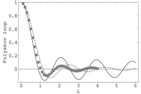
Figure 2: Polyakov loop in the case $D=4$ and $N=\infty$. The dotted line shows the contribution from the zeroth order alone, and the solid line shows that up to the second order. The gray boxes indicate some points of the numerical data for the $N=48$ case in Figure 13 in ref. [17].

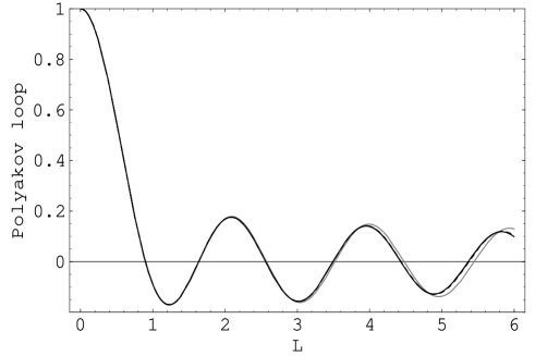
Figure 3: Polyakov loops up to the second order for $(D,N)=(4,16)$, $(4,48)$, $(4,100)$, $(4,400)$ and $(4,\infty)$. The gray line shows the case $(4,16)$, the dotted line $(4,48)$, the dashed line $(4,100)$, the dot-dashed line $(4,400)$, and the solid line $(4,\infty)$.

Since we have obtained the concrete formula for general $D$ and $N$, investigating the behavior for other $D$’s can be immediately done. For example, we plot the $D=10$ case and the $D=26$ case for various $N$’s in Fig. 4. Both casess still exhibit quite good scaling behaviors. As $D$ increases, the curve tends to broaden and to make the amplitude of the oscillation decreased. We can understand the tendency by seeing the large $N$ result (4.70). The former can be understood from the fact that $L$ is contained only through the combination of $\alpha$, and the latter from the suppression of the second term when $D$ being large.

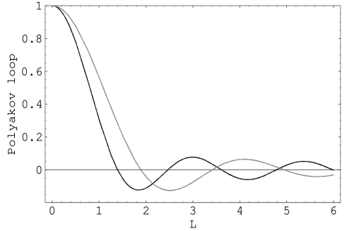
Figure 4: Polyakov loops up to the second order for $(D,N)=(10,48)$, $(10,100)$, $(10,400)$, $(10,\infty)$, $(26,48)$, $(26,100)$, $(26,400)$ and $(26,\infty)$. The dotted line shows the case $(10,48)$, the dashed line $(10,100)$, the dot-dashed line $(10,400)$, the solid line $(10,\infty)$, the gray dotted line $(26,48)$, the gray dashed line $(26,100)$, the gray dot-dashed line $(26,400)$, and the gray solid line $(26,\infty)$.

Thus we have seen that the Gaussian approximation reproduces well the numerical result of the Polyakov loop in smaller $L$ region. How about the Polyakov loop in larger $L$ region? From the same reason as the case of the simple example in section 2, the Gaussian approximation can not be trusted. In section 5, we will consider it by using the improved mean field approximation, and derive the asymptotic behavior of the Polyakov loop approximately.

4.3 Wilson Loop

We consider the expectation value of the rectangular Wilson loop of the size $L\times L$: $\hat{W}(L)=\frac{1}{N}{\rm tr}(e^{iLX_{1}}e^{iLX_{2}}e^{-iLX_{1}}e^{-iLX_{2}})$. Here we evaluate the first two terms in the expansion:

$$\langle\hat{W}(L)\rangle=\langle\hat{W}(L)\rangle_{0}+\sum_{n=1}^{\infty}\frac{(-1)^{n}}{n!}\langle(S-S_{0})^{n}\hat{W}(L)\rangle_{C,0}.$$ (4.71)

Leading Order Term

First let us evaluate the leading (zeroth) order term $\langle\hat{W}(L)\rangle_{0}$, which is written as

$$\langle\hat{W}(L)\rangle_{0}=\frac{1}{N}I(L)_{ijkl}I(L)_{jkli},$$ (4.72)

with $I(L)_{ijkl}\equiv\langle(e^{iLX_{1}})_{ij}(e^{-iLX_{1}})_{kl}\rangle_{0}$. From the invariance of the measure $[dX_{1}]$ under $X_{1}\rightarrow UX_{1}U^{\dagger}$ with $U$ being an arbitrary $SU(N)$ matrix, the quantity $I(L)_{ijkl}$ must satisfy

$$I(L)_{ijkl}=U_{ii^{\prime}}(U^{\dagger})_{j^{\prime}j}U_{kk^{\prime}}(U^{\dagger})_{l^{\prime}l}I(L)_{i^{\prime}j^{\prime}k^{\prime}l^{\prime}}.$$ (4.73)

It determines the structure of the indices of $I(L)_{ijkl}$ as

$$I(L)_{ijkl}=A(L)\delta_{ij}\delta_{kl}+B(L)\delta_{il}\delta_{jk},$$ (4.74)

where $A(L)$ and $B(L)$ are $SU(N)$-invariant. Noting $I(L)_{ijjl}=\delta_{il}$ and $I(L)_{ijki}=\delta_{jk}$, $A(L)$ and $B(L)$ are determined. Thus we can rewrite $\langle\hat{W}(L)\rangle_{0}$ in terms of correlators in the Gaussian one-matrix model:

$$\langle\hat{W}(L)\rangle_{0}=1-\frac{N^{2}}{N^{2}-1}\left[\langle\frac{1}{N}{\rm tr}e^{iLX_{1}}\frac{1}{N}{\rm tr}e^{-iLX_{1}}\rangle_{0}-1\right]^{2}.$$ (4.75)

Considering the integral over the hermitian matrix $Y$ as before, the above correlator can be evaluated, and we obtain the expression

$$\langle\hat{W}(L)\rangle_{0}=1-\frac{N^{2}}{N^{2}-1}\left[-1+\frac{1}{N}+\frac{2}{N^{2}}e^{-\frac{L^{2}\sigma^{2}}{2}}f(L^{2}\sigma^{2})\right]^{2},$$ (4.76)

where $f(x)$ is a polynomial of $x$ given by

$$f(x) \equiv \sum_{n=1}^{N-1}\sum_{m=0}^{n-1}n!m!\left[\left\{\sum_{k=0}^{n}\frac{1}{(k!)^{2}(n-k)!}\left(-\frac{x}{2}\right)^{k}\right\}\left\{\sum_{l=0}^{m}\frac{1}{(l!)^{2}(m-l)!}\left(-\frac{x}{2}\right)^{l}\right\}\right.$$ (4.77)

$$-\left.\left(\frac{x}{2}\right)^{n-m}\left\{\sum_{k=0}^{m}\frac{1}{k!(n-m+k)!(m-k)!}\left(-\frac{x}{2}\right)^{k}\right\}^{2}\right].$$

First Order Term

Next, we compute the first order term $-\langle(S-S_{0})\hat{W}(L)\rangle_{C,0}$. After integrating out the variables other than $X_{1}$ and $X_{2}$, we have

$$-\langle(S-S_{0})\hat{W}(L)\rangle_{C,0}=(N^{2}-1)\left[\frac{\sigma^{4}}{4g^{2}}N(2D-3)-1\right]\langle\hat{W}(L)\rangle_{0}$$ (4.78)

$$-\left[\frac{\sigma^{2}}{2g^{2}}N(D-2)-\frac{1}{\sigma^{2}}\right]\left\{\langle{\rm tr}(X_{1})^{2}\hat{W}(L)\rangle_{0}+\langle{\rm tr}(X_{2})^{2}\hat{W}(L)\rangle_{0}\right\}$$

$$-\frac{1}{g^{2}}\langle(X_{1}X_{1})_{ij}(X_{2}X_{2})_{ji}\hat{W}(L)\rangle_{0}+\frac{1}{g^{2}}\langle(X_{1})_{ij}(X_{1})_{kl}(X_{2})_{jk}(X_{2})_{li}\hat{W}(L)\rangle_{0}.$$

Noting the $SU(N)$-transformation property as in the case of $I(L)_{ijkl}$, the calculation of the correlators in the r.h.s. is reduced to the following more fundamental quantities:

$$f_{1}(L)\equiv\langle\frac{1}{N}{\rm tr}((X_{1})^{2}e^{iLX_{1}})\frac{1}{N}{\rm tr}e^{-iLX_{1}}\rangle_{0},$$

$$f_{2}(L)\equiv\langle\frac{1}{N}{\rm tr}(X_{1})^{2}\frac{1}{N}{\rm tr}e^{iLX_{1}}\frac{1}{N}{\rm tr}e^{-iLX_{1}}\rangle_{0},$$

$$f_{3}(L)\equiv\langle\frac{1}{N}{\rm tr}(X_{1}e^{iLX_{1}})\frac{1}{N}{\rm tr}(X_{1}e^{-iLX_{1}})\rangle_{0}.$$ (4.79)

The result is

$$\langle{\rm tr}(X_{1})^{2}\hat{W}(L)\rangle_{0}=\langle{\rm tr}(X_{2})^{2}\hat{W}(L)\rangle_{0}=\frac{1}{2}\sigma^{2}(N^{2}-1)$$ (4.80)

$$+ \left\{\frac{1}{2}\sigma^{2}N^{2}-\frac{N^{3}}{N^{2}-1}f_{2}(L)\right\}\left[-1+\frac{1}{N}+\frac{2}{N^{2}}e^{-\frac{L^{2}\sigma^{2}}{2}}f(L^{2}\sigma^{2})\right],$$

$$\langle(X_{1}X_{1})_{ij}(X_{2}X_{2})_{ji}\hat{W}(L)\rangle_{0} = -\frac{1}{4}\sigma^{4}\frac{N^{2}-1}{N}+\sigma^{2}N^{2}f_{2}(L)-\frac{N^{3}}{N^{2}-1}(f_{2}(L))^{2}$$ (4.81)

$$-\frac{4N^{3}}{(N^{2}-1)(N^{2}-4)}(f_{1}(L)-f_{2}(L))^{2},$$

$$\langle(X_{1})_{ij}(X_{1})_{kl}(X_{2})_{jk}(X_{2})_{li}\hat{W}(L)\rangle_{0}=\frac{3}{4}\sigma^{4}\frac{N^{2}-1}{N(N^{2}-9)}$$ (4.82)

$$-4\sigma^{2}\frac{N^{2}+6}{(N^{2}-4)(N^{2}-9)}f_{1}(L)-\sigma^{2}\frac{N^{2}(N^{2}-14)}{(N^{2}-4)(N^{2}-9)}f_{2}(L)-6\sigma^{2}\frac{1}{N^{2}-9}f_{3}(L)$$

$$+\frac{24N(N^{2}+1)}{(N^{2}-1)(N^{2}-4)(N^{2}-9)}(f_{1}(L))^{2}-\frac{40N^{3}}{(N^{2}-1)(N^{2}-4)(N^{2}-9)}f_{1}(L)f_{2}(L)$$

$$+\frac{N^{3}(N^{2}+6)}{(N^{2}-1)(N^{2}-4)(N^{2}-9)}(f_{2}(L))^{2}+\frac{16N(2N^{2}-3)}{(N^{2}-1)(N^{2}-4)(N^{2}-9)}f_{1}(L)f_{3}(L)$$

$$-\frac{20N^{3}}{(N^{2}-1)(N^{2}-4)(N^{2}-9)}f_{2}(L)f_{3}(L)+\frac{2N(N^{2}-3)}{(N^{2}-1)(N^{2}-9)}(f_{3}(L))^{2}.$$

Now, what is needed for giving the expression of the first order term is to know the three quantities $f_{1}(L)$, $f_{2}(L)$ and $f_{3}(L)$. We pass to the Gaussian integral of the hermitian matrix $Y$ to evaluate them. Going along the same line as before, we obtain the following formulas:

$$f_{1}(L)=\frac{\sigma^{2}}{2}\frac{N^{2}-1}{N^{2}}$$ (4.83)

$$+ \frac{\sigma^{2}}{2N^{2}}e^{-\frac{L^{2}\sigma^{2}}{2}}\sum_{(n\neq m)\;n,m=0}^{N-1}\left\{\left(4n+1-\frac{L^{2}\sigma^{2}}{2}-\frac{1}{N}\right)F\left(-n,1;\frac{L^{2}\sigma^{2}}{2}\right)\right.$$

$$-4nF\left(-n+1,1;\frac{L^{2}\sigma^{2}}{2}\right)-2n^{2}\frac{L^{2}\sigma^{2}}{2}F\left(-n+2,3;\frac{L^{2}\sigma^{2}}{2}\right)+4nF\left(-n+2,2;\frac{L^{2}\sigma^{2}}{2}\right)$$

$$\left.-2nF\left(-n+1,2;\frac{L^{2}\sigma^{2}}{2}\right)\right\}F\left(-m,1;\frac{L^{2}\sigma^{2}}{2}\right)$$

$$+ \frac{\sigma^{2}}{N^{2}}e^{-\frac{L^{2}\sigma^{2}}{2}}\sum_{n=1}^{N-1}\sum_{m=0}^{n-1}\frac{n!}{m!}\frac{1}{((n-m)!)^{2}}\left\{\left(\frac{L^{2}\sigma^{2}}{2}\right)^{n-m+1}F\left(-m,n-m+1;\frac{L^{2}\sigma^{2}}{2}\right)\right.$$

$$-\left(\frac{L^{2}\sigma^{2}}{2}\right)^{n-m}\left(2n+2m+1-\frac{1}{N}\right)F\left(-m,n-m+1;\frac{L^{2}\sigma^{2}}{2}\right)$$

$$+\left(\frac{L^{2}\sigma^{2}}{2}\right)^{n-m}\frac{2m}{n-m+1}F\left(-m+1,n-m+2;\frac{L^{2}\sigma^{2}}{2}\right)$$

$$\left.+\left(\frac{L^{2}\sigma^{2}}{2}\right)^{n-m-1}(n-m)(n-m-1)F\left(-m,n-m+1;\frac{L^{2}\sigma^{2}}{2}\right)\right\}$$

$$\times F\left(-m,n-m+1;\frac{L^{2}\sigma^{2}}{2}\right),$$

$$f_{2}(L)=\frac{N^{2}-1}{2N}\sigma^{2}\left[\frac{1}{N}+\frac{2}{N^{2}}e^{-\frac{L^{2}\sigma^{2}}{2}}f(L^{2}\sigma^{2})\right]$$ (4.84)

$$+ \frac{\sigma^{2}}{N^{3}}e^{-\frac{L^{2}\sigma^{2}}{2}}\sum_{n,m=0}^{N-1}\left\{-\frac{L^{2}\sigma^{2}}{2}F\left(-n,1;\frac{L^{2}\sigma^{2}}{2}\right)+2(n-1)\frac{L^{2}\sigma^{2}}{2}F\left(-n+2,2;\frac{L^{2}\sigma^{2}}{2}\right)\right.$$

$$-2F\left(-n+2,2;\frac{L^{2}\sigma^{2}}{2}\right)+n\frac{L^{2}\sigma^{2}}{2}F\left(-n+2,3;\frac{L^{2}\sigma^{2}}{2}\right)$$

$$\left.+2\left(\frac{L^{2}\sigma^{2}}{2}+1\right)F\left(-n+1,1;\frac{L^{2}\sigma^{2}}{2}\right)-4n\frac{L^{2}\sigma^{2}}{2}F\left(-n+1,2;\frac{L^{2}\sigma^{2}}{2}\right)\right\}F\left(-m,1;\frac{L^{2}\sigma^{2}}{2}\right)$$

$$- \frac{\sigma^{2}}{N^{3}}e^{-\frac{L^{2}\sigma^{2}}{2}}\sum_{n=0}^{N-1}\left\{-\frac{L^{2}\sigma^{2}}{2}F\left(-n,1;\frac{L^{2}\sigma^{2}}{2}\right)-2nF\left(-n+1,2;\frac{L^{2}\sigma^{2}}{2}\right)+2nF\left(-n,1;\frac{L^{2}\sigma^{2}}{2}\right)\right.$$

$$\left.-2\left(\frac{L^{2}\sigma^{2}}{2}+1\right)F\left(2,2;\frac{L^{2}\sigma^{2}}{2}\right)+2F\left(2,1;\frac{L^{2}\sigma^{2}}{2}\right)\right\}F\left(-n,1;\frac{L^{2}\sigma^{2}}{2}\right)$$

$$+ \frac{\sigma^{2}}{N^{3}}e^{-\frac{L^{2}\sigma^{2}}{2}}2\sum_{n=1}^{N-1}\sum_{m=0}^{n-1}\frac{n!}{m!}\frac{1}{((n-m)!)^{2}}\left\{\left(\frac{L^{2}\sigma^{2}}{2}\right)^{n-m+1}F\left(-m,n-m+1;\frac{L^{2}\sigma^{2}}{2}\right)\right.$$

$$-\left(\frac{L^{2}\sigma^{2}}{2}\right)^{n-m}(n+m)F\left(-m,n-m+1;\frac{L^{2}\sigma^{2}}{2}\right)$$

$$+\left(\frac{L^{2}\sigma^{2}}{2}\right)^{n-m}\frac{2m}{n-m+1}F\left(-m+1,n-m+2;\frac{L^{2}\sigma^{2}}{2}\right)$$

$$\left.+\left(\frac{L^{2}\sigma^{2}}{2}\right)^{n-m-1}(n-m)(n-m-1)F\left(-m,n-m+1;\frac{L^{2}\sigma^{2}}{2}\right)\right\}$$

$$\times F\left(-m,n-m+1;\frac{L^{2}\sigma^{2}}{2}\right)$$

$$+ \frac{\sigma^{2}}{N^{3}}e^{-\frac{L^{2}\sigma^{2}}{2}}2\sum_{n=2}^{N-1}\sum_{m=1}^{n-1}\frac{n!}{m!}\frac{1}{(n-m+1)!(n-m-1)!}\left(\frac{L^{2}\sigma^{2}}{2}\right)^{n-m}$$

$$\times\left\{\left(\frac{L^{2}\sigma^{2}}{2}-n-m\right)F\left(-m,n-m;\frac{L^{2}\sigma^{2}}{2}\right)+(n-m)F\left(-m-1,n-m;\frac{L^{2}\sigma^{2}}{2}\right)\right\}$$

$$\times F\left(-m+1,n-m+2;\frac{L^{2}\sigma^{2}}{2}\right)$$

$$+ \frac{\sigma^{2}}{N^{3}}e^{-\frac{L^{2}\sigma^{2}}{2}}2\sum_{n=0}^{N-3}(n+2)(n+1)\frac{L^{2}\sigma^{2}}{2}F\left(-n-1,2;\frac{L^{2}\sigma^{2}}{2}\right)F\left(-n,2;\frac{L^{2}\sigma^{2}}{2}\right),$$

$$f_{3}(L)=\frac{\sigma^{2}}{2}\frac{N^{2}-1}{N^{2}}$$ (4.85)

$$+ \frac{\sigma^{2}}{N^{3}}e^{-\frac{L^{2}\sigma^{2}}{2}}\sum_{n=1}^{N-1}\sum_{m=0}^{n-1}\left[\frac{L^{2}\sigma^{2}}{2}N\left\{F\left(-n,1;\frac{L^{2}\sigma^{2}}{2}\right)+2nF\left(-n+1,2;\frac{L^{2}\sigma^{2}}{2}\right)\right\}\right.$$

$$\left.\times\left\{F\left(-m,1;\frac{L^{2}\sigma^{2}}{2}\right)+2mF\left(-m+1,2;\frac{L^{2}\sigma^{2}}{2}\right)\right\}-F\left(-n,1;\frac{L^{2}\sigma^{2}}{2}\right)F\left(-m,1;\frac{L^{2}\sigma^{2}}{2}\right)\right]$$

$$- \frac{\sigma^{2}}{N^{3}}e^{-\frac{L^{2}\sigma^{2}}{2}}\sum_{n=1}^{N-1}\sum_{m=0}^{n-1}\frac{n!}{m!}\frac{1}{((n-m)!)^{2}}\left(\frac{L^{2}\sigma^{2}}{2}\right)^{n-m-1}$$

$$\times\left[N\left\{\left(\frac{L^{2}\sigma^{2}}{2}-n-m\right)F\left(-m,n-m+1;\frac{L^{2}\sigma^{2}}{2}\right)+2mF\left(-m+1,n-m+1;\frac{L^{2}\sigma^{2}}{2}\right)\right\}^{2}\right.$$

$$\left.-\frac{L^{2}\sigma^{2}}{2}\left\{F\left(-m,n-m+1;\frac{L^{2}\sigma^{2}}{2}\right)\right\}^{2}\right].$$

We used some recursion relations among confluent hypergeometric functions for later convenience in considering the large $N$ limit.

Gaussian Approximation

We consider the above result at the value (4.2) to obtain the Wilson loop amplitude up to the first order in the Gaussian approximation. Since the formula is quite lengthy, we do not write down here directly. Instead, we plot the result in the case of various values of $D$ and $N$ below. As in the case of the Polyakov loop, the large $N$ limit also yields the result remarkably simplified as

$$\langle\hat{W}(L)\rangle=1-\left(\frac{1}{\alpha}(J_{1}(2\sqrt{\alpha}))^{2}-1\right)^{2}$$ (4.86)

$$+\frac{1}{D-1}\frac{2}{\alpha^{2}}\left(9(J_{1}(2\sqrt{\alpha}))^{2}(J_{3}(2\sqrt{\alpha}))^{2}+8(J_{2}(2\sqrt{\alpha}))^{4}\right)+O((S-S_{0})^{2}).$$

The first line and the first term in the second line in the r.h.s. represent the contributions from the leading order term and from the first order term, respectively. The factor $\frac{1}{D-1}$ in the second line means the validity of the interpretation as the mean field approximation.

In the $D=4$ case, it is interesting to compare our result with the numerical calculation reported in ref. [17]. Figure 11 in ref. [17] is the result to be compared with ours. As in the case of the Polyakov loop, we take $Ng^{2}=48$ for the common setting. In Fig. 5 we show the result of the leading order alone and that summed up to the first order when $N=16$. It can be seen that the result up to the first order match well with the numerical result. (See also Fig. 6.) We similarly plot the result for the case $N=\infty$ in Fig. 6. Comparing this with Fig. 5, we expect a good scaling behavior in the region of smaller $L$. In fact, Fig. 7 shows the behaviors for $N=16$, 48 and $\infty$ together, from which the scaling for smaller $L$ can be observed. In particular, the scaling between the cases of $N=48$ and $N=\infty$ is too good to distinguish each curve in the region $L<4$. These scaling behaviors are in conformity with the numerical result in ref. [17].

Figure 5: Wilson loop in the case $D=4$ and $N=16$. The dotted line shows the contribution from the zeroth order alone, and the solid line shows that up to the first order.

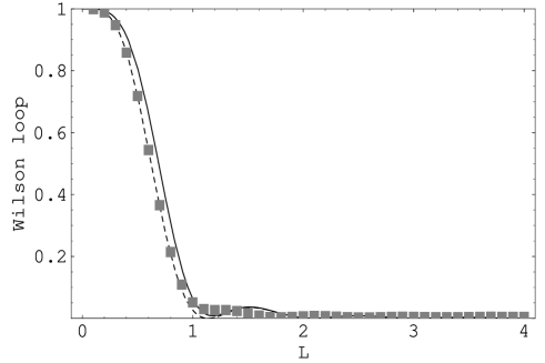
Figure 6: Wilson loop for $D=4$, $N=\infty$ case. The dotted line shows the contribution from the zeroth order alone, and the solid line shows that up to the first order. The gray boxes indicate some points of the numerical data for the $N=48$ case in Figure 11 in ref. [17].

Figure 7: Wilson loops up to the first order for $(D,N)=(4,16)$, $(4,48)$ and $(4,\infty)$. The dotted line shows the case $(4,16)$, the dashed line $(4,48)$ and the solid line $(4,\infty)$.

As in the case of the Polyakov loop, we depict the behaviors for $D=10$ and 26 in Fig. 8. We can still see quite good scaling behaviors. Also, from Fig. 7 and Fig. 8, it can be seen that the curve tends to become broader as $D$ increases. The tendency can be understood from the formula in the large $N$ limit (4.86), where $L$ appears only through the combination of $\alpha$.

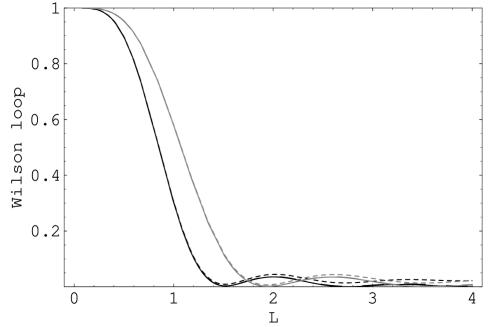
Figure 8: Wilson loops up to the first order for $(D,N)=(10,16)$, $(10,48)$, $(10,\infty)$, $(26,16)$, $(26,48)$ and $(26,\infty)$. The dotted line shows the case $(10,16)$, the dashed line $(10,48)$, the solid line $(10,\infty)$, the gray dotted line $(26,16)$, the gray dashed line $(26,48)$, and the gray solid line $(26,\infty)$.

5 Reduced Yang-Mills Integrals — Improved Mean Field Approximation

In this section we evaluate the expectation values for the space-time extent, the Polyakov loop and the Wilson loop by the method of the improved mean field approximation. For the space-time extent, it turns out to give a result closer to the exact value than the Gaussian approximation in the case of $N=2$. Furthermore, for the Polyakov loop and the Wilson loop, it yields the asymptotic behaviors for the large loop. Although we consider only the first few terms in the expansion around the mean field configuration, as we have done in section 2.2, it can be guessed to give the results which reproduce the correct behaviors at least qualitatively.

Let us consider the improved mean field approximation in the reduced Yang-Mills integrals for the operator ${\cal O}$ which is $U(N)$-invariant and isotropic in $D$-dimensional space. We start with the mean field action

$$S_{M}=\frac{1}{2g^{2}}\sum_{\mu\neq\nu}2\left[-\langle(X_{\mu})_{ij}(X_{\mu})_{kl}\rangle^{{\cal O}}(X_{\nu})_{jk}(X_{\nu})_{li}+\langle(X_{\mu})_{ij}(X_{\mu})_{jk}\rangle^{{\cal O}}(X_{\nu})_{kl}(X_{\nu})_{li}\right]+\frac{1}{\tilde{\lambda}}.$$ (5.1)

Since ${\cal O}$ is $U(N)$-invariant,

$$\langle(X_{\mu})_{ij}(X_{\mu})_{kl}\rangle^{{\cal O}}\equiv\frac{\int(dX)\;e^{-S}(X_{\mu})_{ij}(X_{\mu})_{kl}{\cal O}}{\int(dX)\;e^{-S}{\cal O}}\propto\delta_{il}\delta_{jk}-\frac{1}{N}\delta_{ij}\delta_{kl}.$$ (5.2)

Also, due to the isotropic nature, the proportional constant in the above is independent of $\mu$. So the action $S_{M}$ can be written as the standard form $S_{M}=\frac{1}{\tilde{\sigma}^{2}}{\rm tr}(X_{\mu})^{2}+\frac{1}{\tilde{\lambda}}$ with

$$\frac{1}{\tilde{\sigma}^{2}}=\frac{1}{g^{2}}\frac{D-1}{D}\frac{N^{2}}{N^{2}-1}\langle\frac{1}{N}{\rm tr}(X_{\mu})^{2}\rangle^{{\cal O}}.$$ (5.3)

The self-consistency condition $\langle\frac{1}{N}{\rm tr}(X_{\mu})^{2}\rangle^{{\cal O}}=\langle\frac{1}{N}{\rm tr}(X_{\mu})^{2}\rangle^{{\cal O}}_{M}$ reads

$$\frac{1}{\tilde{\sigma}^{2}}g^{2}\frac{D}{D-1}\frac{N^{2}-1}{N^{2}}=\frac{\langle\frac{1}{N}{\rm tr}(X_{\mu})^{2}{\cal O}\rangle_{M}}{\langle{\cal O}\rangle_{M}},$$ (5.4)

which determines $\tilde{\sigma}$. As before, $\tilde{\lambda}$ is given by the formula of the same form as (2.22) with $S^{\prime}_{M}=\frac{1}{\tilde{\sigma}^{2}}{\rm tr}(X_{\mu})^{2}$.

5.1 Space-Time Extent

Now we consider the case ${\cal O}=\frac{1}{N}{\rm tr}(X_{\mu})^{2}$. From (5.4), we have

$$\tilde{\sigma}^{2}=\sqrt{\frac{2g^{2}}{N(D-1)}}\left[1+\frac{2}{(N^{2}-1)D}\right]^{-1/2}.$$ (5.5)

Up to the second order with respect to $S-S^{\prime}_{M}$, $\tilde{\lambda}$ becomes

$$\frac{1}{\tilde{\lambda}} = \frac{3\tilde{\sigma}^{4}}{8g^{2}}N(N^{2}-1)D(D-1)-\frac{3}{4}(N^{2}-1)D+\frac{3\tilde{\sigma}^{4}}{2g^{2}}N(D-1)-\frac{3}{2}$$ (5.6)

$$-\frac{\tilde{\sigma}^{8}}{64g^{4}}N^{2}(N^{2}-1)D(D-1)(4D-1)-\frac{3\tilde{\sigma}^{8}}{8g^{4}}N^{2}D(D-1)+O((S-S^{\prime}_{M})^{3}).$$

Following the steps in section 2.2, we obtain the expectation value

$$\langle\frac{1}{N}{\rm tr}(X_{\mu})^{2}\rangle=\sqrt{\frac{Ng^{2}}{2(D-1)}}\frac{N^{2}-1}{N^{2}}D\left[1+\frac{2}{(N^{2}-1)D}\right]^{-\frac{1}{4}(N^{2}-1)D-\frac{1}{2}}$$ (5.7)

$$\times\exp\left\{\left[\frac{1}{2}+\frac{3}{4(D-1)}+\frac{2}{(N^{2}-1)D}-\frac{3}{4(D-1)}\frac{1}{(N^{2}-1)D}+\frac{6}{(N^{2}-1)^{2}D^{2}}\right]\right.$$

$$\hskip 56.9055pt\times\left.\left[1+\frac{2}{(N^{2}-1)D}\right]^{-2}\right\}$$

$$\times[1+O((S-S^{\prime}_{M})^{3})].$$

Then, in the case of $N=2$ and $D$ large, it has the following expansion:

$$\langle\frac{1}{2}{\rm tr}(X_{\mu})^{2}\rangle=\frac{3g}{4}\sqrt{D}\left[1+\frac{13}{12D}+O(D^{-2})+O((S-S^{\prime}_{M})^{3})\right].$$ (5.8)

Here, it is noted that this result fits the exact result (4.11) better than the case of the Gaussian approximation (4.10). So, this scheme can be expected to give an improved result also for other $N$. Moreover, there is another comment. If we stopped the computation up to the first order, we would end up with the expansion

$$\langle\frac{1}{2}{\rm tr}(X_{\mu})^{2}\rangle=\frac{3g}{4}\sqrt{D}\left[1+\frac{2}{3D}+O(D^{-2})+O((S-S^{\prime}_{M})^{2})\right].$$ (5.9)

Thus, we can see that in the $SU(2)$ case the result approaches closer to the exact result as increasing the order of the approximation. For general $N$, we can compare with the $1/D$-expansion result (3.6). Normalizing the leading term to the unity, we have the following coefficients in the $O(D^{-1/2})$-terms:

$$\begin{array}[]{ll}2&:\mbox{Gaussian approximation up to the 2nd order}\\ \frac{5}{4}-\frac{1}{2(N^{2}-1)}&:\mbox{Improved mean field approximation up to the 2nd order}\\ \frac{1}{2}+\frac{1}{2(N^{2}-1)}&:\mbox{Improved mean field approximation up to the 1st order}\\ \frac{7}{6}+\frac{1}{N^{2}-1}&:\mbox{$1/D$-expansion method},\end{array}$$ (5.10)

which exhibits a similar tendency as seen in the $N=2$ case. Thus it can be expected that the expansion with respect to $S-S^{\prime}_{M}$ based on the improved mean field approximation does work for general $N$.

5.2 Polyakov Loop

Here we consider the case ${\cal O}=\frac{1}{2D}\sum_{\mu=1}^{D}\frac{1}{N}{\rm tr}(e^{iLX_{\mu}}+e^{-iLX_{\mu}})$, whose expectation value is equal to $\langle\hat{P}(L)\rangle$ if $O(D)$-symmetry is not broken spontaneously. In the case that $N$ and $D$ are finite, it always holds. Let us consider this case. For this ${\cal O}$, the method in the beginning of this section can be used. Now, eq. (5.4) leads

$$\frac{1}{\tilde{\sigma}^{2}}g^{2}\frac{D}{D-1}\frac{N^{2}-1}{N^{2}} = -\frac{L^{2}\tilde{\sigma}^{4}}{4}\frac{N+1}{N}\frac{F\left(1-N,3;\frac{L^{2}\tilde{\sigma}^{2}}{2}\right)}{F\left(1-N,2;\frac{L^{2}\tilde{\sigma}^{2}}{2}\right)}$$ (5.11)

$$+\left(\frac{1}{2}(N^{2}-1)D+\frac{L^{2}\tilde{\sigma}^{2}}{4}\frac{N+1}{N}\right)\frac{\tilde{\sigma}^{2}}{N}.$$

We are interested in the case of $L^{2}g$ and $x\equiv L^{2}\tilde{\sigma}^{2}$ large. In this case, the ratio between the confluent hypergeometric functions is expanded as

$$\frac{F\left(1-N,3;\frac{x}{2}\right)}{F\left(1-N,2;\frac{x}{2}\right)}=\frac{2}{N+1}\left[1-(N-1)\frac{2}{x}-N(N-1)\frac{4}{x^{2}}+O(x^{-3})\right],$$

so the above equation has the form

$$-\frac{g^{2}L^{4}}{x^{2}}\frac{D}{D-1}\frac{1}{N}=\frac{1}{4N(N+1)}x-\frac{1}{2}D-\frac{1}{N+1}-\frac{2N}{N+1}\frac{1}{x}+O(x^{-2}).$$ (5.12)

We iteratively solve this equation and get the three solutions:

$$x_{\pm} = e^{\pm\pi i/3}\left(\frac{4D}{D-1}(N+1)L^{4}g^{2}\right)^{1/3}+\frac{2}{3}N((N+1)D+2)+O((L\sqrt{g})^{-4/3}),$$

$$x_{0} = -\left(\frac{4D}{D-1}(N+1)L^{4}g^{2}\right)^{1/3}+\frac{2}{3}N((N+1)D+2)+O((L\sqrt{g})^{-4/3}).$$ (5.13)

Corresponding to each $x$, $\tilde{\lambda}$ is determined by

$$\frac{1}{\tilde{\lambda}}=(N-1)\left\{\frac{1}{4N}x-1+O(x^{-1})+O((S-S^{\prime}_{M})^{2})\right\}$$ (5.14)

up to the first order with respect to $S-S^{\prime}_{M}$, and

$$\frac{1}{\tilde{\lambda}} = (N-1)\left\{\frac{1}{2N}x-\frac{1}{8}(N+1)(N-9)D-\frac{1}{8}(N+1)^{2}\frac{D}{D-1}-\frac{3}{2}\right.$$ (5.15)

$$\left.+O(x^{-1})+O((S-S^{\prime}_{M})^{3})\right\}$$

up to the second order. Eq. (5.12) was used for making the expressions simpler. It is noted that the situation here is very similar to that in section 2.2. Applying the same recipe as in section 2.2, we end up with the final expression:

$$\langle\hat{P}(L)\rangle = C_{(n)}(L^{4}g^{2})^{-\frac{1}{12}(N-1)((N+1)D-4)}\exp\left[-u_{(n)}\frac{N-1}{N}\left(\frac{4D}{D-1}(N+1)L^{4}g^{2}\right)^{1/3}\right]$$ (5.16)

$$\times\cos\left[\sqrt{3}u_{(n)}\frac{N-1}{N}\left(\frac{4D}{D-1}(N+1)L^{4}g^{2}\right)^{1/3}-\frac{\pi}{6}(N-1)((N+1)D+2)\right]$$

$$\times[1+O((L^{4}g^{2})^{-1/3})+O((S-S^{\prime}_{M})^{n+1})],$$

where up to the first order ($n=1$): $u_{(1)}=\frac{1}{4}$, and up to the second order ($n=2$): $u_{(2)}=\frac{3}{8}$. The overall constants are

$$C_{(1)} = \frac{(-1)^{N-1}}{2^{N-2}N!}\left(\frac{N}{2}(D-1)\right)^{\frac{1}{4}(N^{2}-1)D}\left(\frac{4D}{D-1}(N+1)\right)^{\frac{1}{6}(N-1)((N+1)D+2)}$$

$$\times\exp\left[-\frac{7}{12}(N^{2}-1)D+\frac{1}{3}(N-1)\right],$$

$$C_{(2)} = \frac{(-1)^{N-1}}{2^{N-2}N!}\left(\frac{N}{2}(D-1)\right)^{\frac{1}{4}(N^{2}-1)D}\left(\frac{4D}{D-1}(N+1)\right)^{\frac{1}{6}(N-1)((N+1)D+2)}$$

$$\times\exp\left[\frac{1}{8}(N^{2}-1)(N+1)\frac{D^{2}}{D-1}-2(N^{2}-1)D-\frac{3}{16}(N^{2}-1)\frac{D}{D-1}+\frac{1}{2}(N-1)\right].$$

At present, we have no result of the computer simulation for the behavior in the region of $L^{2}g$ large. However, our result can be expected to represent the behavior correctly at least qualitatively. It seems interesting to consider our result together with the asymptotic behavior of the eigenvalue density $\rho(\lambda)$ (3.5). In fact, $\rho(\lambda)$ can be obtained from $\langle\hat{P}(L)\rangle$ via the Fourier transformation:

$$\rho(\lambda)=\int_{-\infty}^{\infty}\frac{dL}{2\pi}\;e^{-iL\lambda}\langle\hat{P}(L)\rangle.$$

If we tried to evaluate the integral in the r.h.s. for $\lambda$ large by the saddle point approximation using the formula of (5.16), it would turn out that the width of the Gaussian integral around the saddle point becomes infinitely large as $\lambda\rightarrow\infty$. It indicates that we should take into account the contribution infinitely far away from the saddle point, and thus that in this case the saddle point approximation is inadequate. We need the information of $\langle\hat{P}(L)\rangle$ for the whole range of $L$ to get the asymptotic behavior of $\rho(\lambda)$.

Also, we can consider the improvement of the result in the region of smaller $L^{2}g$ in the previous section by using this method similarly as in the case of the space-time extent in the previous subsection. Since it is considered not to change the result essentially, we do not present here.

5.3 Wilson Loop

We analyze the expectation value of the Wilson loop for the case of the length of the loop $L$ large in the improved mean field approximation. Doing the same procedure as before for the operator

$${\cal O}=\frac{1}{D(D-1)}\sum_{\mu\neq\nu}\frac{1}{N}{\rm tr}\left(e^{iLX_{\mu}}e^{iLX_{\nu}}e^{-iLX_{\mu}}e^{-iLX_{\nu}}\right),$$ (5.17)

we have the following equation for $\tilde{\sigma}$:

$$\frac{1}{\tilde{\sigma}^{2}}g^{2}\frac{D}{D-1}\frac{N^{2}-1}{N^{2}}=\frac{\langle\frac{1}{N}{\rm tr}(X_{\mu})^{2}\hat{W}(L)\rangle_{M}}{\langle\hat{W}(L)\rangle_{M}},$$ (5.18)

where the r.h.s. can be easily evaluated by using the expressions (4.76) and (4.80) replaced $\sigma$ with $\tilde{\sigma}$. When $L^{2}\tilde{\sigma}^{2}$ and $L^{2}g$ are large, the r.h.s. is expanded as

$$\frac{\langle\frac{1}{N}{\rm tr}(X_{\mu})^{2}\hat{W}(L)\rangle_{M}}{\langle\hat{W}(L)\rangle_{M}}=\frac{D}{2}\tilde{\sigma}^{2}\frac{N^{2}-1}{N}$$ (5.19)

$$+4\tilde{\sigma}^{2}\frac{N-1}{(N!)^{2}}e^{-\frac{L^{2}\tilde{\sigma}^{2}}{2}}\left(\frac{L^{2}\tilde{\sigma}^{2}}{2}\right)^{2N-2}\left[1+O\left(e^{-\frac{L^{2}\tilde{\sigma}^{2}}{2}}(L^{2}\tilde{\sigma}^{2})^{2N-3}\right)\right].$$

So, the solution up to the next-to-leading order becomes

$$\tilde{\sigma}^{2}=\sigma^{2}\left\{1-\frac{4}{(N+1)!(N-1)!}\frac{1}{D}e^{-\frac{L^{2}\sigma^{2}}{2}}\left(\frac{L^{2}\sigma^{2}}{2}\right)^{2N-2}+O\left(e^{-L^{2}\sigma^{2}}(L^{2}\sigma^{2})^{4N-4}\right)\right\},$$ (5.20)

with $\sigma^{2}=\sqrt{\frac{2g^{2}}{N(D-1)}}$. Note that in the $L\rightarrow\infty$ limit $\tilde{\sigma}^{2}$ coincides to the value of $\sigma^{2}$ in the Gaussian approximation. Up to the first order with respect to $S-S^{\prime}_{M}$, $\tilde{\lambda}$ is determined as

$$\frac{1}{\tilde{\lambda}} = \frac{\langle(S-S^{\prime}_{M})\hat{W}(L)\rangle_{M}}{\langle\hat{W}(L)\rangle_{M}}+O((S-S^{\prime}_{M})^{2})$$ (5.21)

$$= -(N^{2}-1)\left\{\frac{D}{4}+\frac{1}{N^{2}(N+3)}\frac{1}{D-1}\right\}$$

$$-\frac{2}{N!(N-2)!}\left\{1+\frac{4}{N^{2}(N+3)}\frac{1}{D}-\frac{2(N+1)(N+6)}{N^{2}(N+2)(N+3)}\frac{1}{D-1}\right\}e^{-\frac{L^{2}\sigma^{2}}{2}}\left(\frac{L^{2}\sigma^{2}}{2}\right)^{2N-2}$$

$$+O\left(e^{-\frac{L^{2}\sigma^{2}}{2}}(L^{2}\sigma^{2})^{2N-3}\right)+O((S-S^{\prime}_{M})^{2}).$$

Plugging these into the unnormalized expectation value $\langle\hat{W}(L)\rangle^{\prime}=(\tilde{\sigma}^{2})^{\frac{1}{2}(N^{2}-1)D}e^{-1/\tilde{\lambda}}\langle\hat{W}(L)\rangle_{M},$ and dividing it by the partition function up to the first order, we end up with the final expression:

$$\langle\hat{W}(L)\rangle=\frac{2}{N+1}\exp\left[\frac{N^{2}-1}{N^{2}(N+3)}\frac{1}{D-1}\right]$$ (5.22)

$$\times \left[1+\frac{1}{N!(N-2)!}\frac{4}{N^{2}(N+3)}\left\{\frac{2}{D}-\frac{(N+1)(N+6)}{N+2}\frac{1}{D-1}\right\}e^{-\frac{L^{2}\sigma^{2}}{2}}\left(\frac{L^{2}\sigma^{2}}{2}\right)^{2N-2}\right.$$

$$\left.+O\left(e^{-\frac{L^{2}\sigma^{2}}{2}}(L^{2}\sigma^{2})^{2N-3}\right)+O((S-S^{\prime}_{M})^{2})\right].$$

There are two comments in order. First, in the above expression, $\langle\hat{W}(L)\rangle$ has a nonzero limit as $L\rightarrow\infty$, which is $\frac{2}{N+1}\exp\left[\frac{N^{2}-1}{N^{2}(N+3)}\frac{1}{D-1}\right]$. The value approaches to zero as increasing $N$. Second, since $\frac{2}{D}-\frac{(N+1)(N+6)}{N+2}\frac{1}{D-1}<0$ for $D>1$, $\langle\hat{W}(L)\rangle$ approaches to the limit from the below. In the analysis of the Wilson loop, because $\tilde{\sigma}$ reduces to $\sigma$ in the $L\rightarrow\infty$ limit, the result in the Gaussian approximation is considered to roughly reproduce the nonzero limit here. In fact, in the $L\rightarrow\infty$ limit the result of the Gaussian approximation becomes

$$\lim_{L\rightarrow\infty}\left[\langle\hat{W}(L)\rangle_{0}-\langle(S-S_{0})\hat{W}(L)\rangle_{C,0}\right]=\frac{2}{N+1}+\frac{2}{D-1}\frac{N-1}{N^{2}(N+3)},$$ (5.23)

which reproduces the expansion of the exponential up to the first order in the limit of (5.22). As is seen from the above formula, this seemingly strange behavior becomes hardly visible as increasing $N$. The phenomenon just like this is reported in ref. [15], where for $N=2$, 4 and 8 cases in the supersymmetric IKKT integral numerical simulations are performed and results similar as ours are obtained (in Fig. 3a in ref. [15]). There, it is interpreted as a finite $N$ artifact, because of the value of the limit decreasing as increasing $N$, which is common to our result. Also, its dependence on the shape of the contour is reported in ref. [15]. That is, when changing the contour from the square to a regular polygon, the value decreases as increasing the number of edges of the polygon.

In this method, we can also consider the improvement of the result presented in the region of $L^{2}g$ smaller in the previous section. Due to the same reasoning as in the case of the Polyakov loop, we do not give here.

6 Discussions

Here, we summarize our results and discuss possible future directions for concluding this paper.

We analyzed the reduced Yang-Mills integrals by using the Gaussian approximation and its improved version, after confirming the validity of the schemes in the simple example of the $\phi^{4}$-integral. The free energy was evaluated approximately. Since the Gaussian approximation can be regarded as the mean field approximation, the approximation is expected to become better as the space-time dimensionality $D$ increases. Actually, for the $SU(2)$ case, where the exact result is known, we can make sure this expectation. Also for several lower $N$’s, comparing with the numerical result, we found a tendency of better agreement not only for larger $D$ but also for larger $N$. Next, we investigated the square of the space-time extent and the one-point functions for the Polyakov loop and the Wilson loop both by the Gaussian approximation and by the improved mean field approximation. In the $SU(2)$ case, we saw that our results for the space-time extent exhibit good agreement with the exact result when $D$ is large. In particular, in the improved mean field approximation, the situation becomes better than that in the Gaussian approximation. We saw that it likely holds for general $N$ by comparing with the $1/D$-expansion result. We evaluated the Polyakov loop and the Wilson loop by the Gaussian approximation when the length of the loop $L$ is smaller, and by the improved mean field approximation when $L$ large. In the former analysis, we saw that our results nicely fit the numerical results in ref. [17]. Furthermore, the remarkably simple formulas were obtained in the ’t Hooft like large $N$ limit. We also observed quite good scaling behaviors in the region $N\geq 48$, which means that in the scaling region the simple formulas represent sufficiently well the behaviors in the case $L$ smaller. In the latter analysis, the result of the Wilson loop is in conformity with the numerical result [25], while with respect to the Polyakov loop we do not have any results to be compared with ours as far as we know. From the analysis for the simple example, however, our results can be expected to reproduce the correct behaviors at least qualitatively.

For possible future directions, we mainly point out the following two issues. One is an extension of this method for supersymmetric systems. Because our motivation is to explore approximation schemes trusted nonperturbatively in the IKKT integral, it is one of the most important issues. As the first step, it will be good to consider $D=4$ supersymmetric case. Since in this case there are nice numerical results in ref. [17], it will be a good test for the approximation. From the analysis for various supersymmetric quantum mechanical systems in the Gaussian approximation in refs. [22, 23], it seems to be necessary to consider the Gaussian approximation after rewriting the system in terms of the superfields. The other is to calculate more general correlators in our framework. In order to use our improved mean field formalism for the one-point functions, we considered the restricted class of the operators with the isotropic nature. Due to this nature, we could use the simple mean field action. For considering general operators, we will need to start with the mean field action with more general form. We hope that the analysis along this line gives any insights for studies of the nonperturbative aspects of string theory.

Acknowledgements

The authors would like to thank M. Staudacher for informing them of the results not reported in literatures and for giving useful comments. Also, they wish to thank the authors of ref. [17], in particular J. Nishimura and W. Bietenholz for comments and sending numerical data in the paper. One of them (F.S.) thanks A. Allahverdyan for explaining about the computer systems at Saclay.

Appendix

Appendix A Improved Mean Field Analysis in $\phi^{6}$-integral

Here we present the improved mean field analysis for $\phi^{6}$-integral as another example which holds the assumption mentioned in section 2.2. We consider the $\phi^{6}$-integral defined by the classical action: $S=\frac{1}{6g^{2}}\phi^{6}$.

A.1 Saddle Point Approximation

First, let us evaluate the integral $\int_{-\infty}^{\infty}d\phi\;e^{-S}e^{iL\phi}$ in the case of $L$ large by the saddle point approximation. The solutions for the saddle point equation and the corresponding values of $-S+iL\phi$ are

$$\phi_{k}=e^{\pi i(4k-3)/10}(Lg^{2})^{1/5},\hskip 56.9055pt(-S+iL\phi)|_{\phi_{k}}=-\frac{5}{6g^{2}}e^{2\pi i(k-2)/5}(Lg^{2})^{6/5},$$ (A.1)

where $k=1,\cdots,5$. Taking into account regions where the integrand does not blow up as $|\phi|\rightarrow\infty$, it turns out that we should deform the integration contour so as to pass the three points $\phi_{1}$, $\phi_{2}$ and $\phi_{3}$ along each steepest descent direction. After the Gaussian integrals, dividing by the partition function

$$Z=\int_{-\infty}^{\infty}d\phi\;e^{-S}=\frac{1}{3}(6g^{2})^{1/6}\Gamma\left(\frac{1}{6}\right),$$ (A.2)

the expectation value becomes

$$\langle e^{iL\phi}\rangle=\frac{1}{Z}\langle e^{iL\phi}\rangle^{\prime}\sim\sqrt{\frac{2\pi}{5}}\frac{3}{6^{1/6}}\frac{1}{\Gamma(\frac{1}{6})}\frac{1}{(Lg^{1/3})^{2/5}}\left\{e^{-\frac{5}{6}(Lg^{1/3})^{6/5}}\frac{}{}\right.$$ (A.3)

$$\left.+2e^{-\frac{5}{6}(\cos\frac{2\pi}{5})(Lg^{1/3})^{6/5}}\cos\left[\frac{5}{6}(\sin\frac{2\pi}{5})(Lg^{1/3})^{6/5}-\frac{\pi}{5}\right]\right\}.$$

A.2 Improved Mean Field Approximation

Next, we consider the mean field treatment for this system. For the partition function, we start with the following mean field action:

$$S_{M}=\frac{1}{6g^{2}}\cdot 15\langle\phi^{4}\rangle\phi^{2}+\frac{1}{\lambda}=\frac{1}{2\sigma^{2}}\phi^{2}+\frac{1}{\lambda}.$$ (A.4)

The self-consistency condition $\langle\phi^{4}\rangle=\langle\phi^{4}\rangle_{M}$ determines $\sigma$ as $\sigma^{2}=\left(\frac{g^{2}}{15}\right)^{1/3}.$ Also, $\lambda$ is given by the same form as (2.18). Calculation of the first few terms in the mean field expansion leads the expression of the free energy:

$$F=-\ln Z=-\frac{1}{6}\ln g^{2}-\frac{1}{2}\ln\frac{2\pi}{15^{1/3}}-\frac{1}{3}-\frac{17}{45}+O(\langle(S-S^{\prime}_{M})^{3}\rangle_{C,M}),$$ (A.5)

where the third and the fourth term in the r.h.s. represent the contribution from $\langle S-S^{\prime}_{M}\rangle_{M}$ and from $\langle(S-S^{\prime}_{M})^{2}\rangle_{C,M}$, respectively.

Now let us discuss the improved version of the mean field approximation for the unnormalized expectation value $\langle e^{iL\phi}\rangle^{\prime}$. Starting with the mean field action

$$S_{M}=\frac{1}{6g^{2}}\cdot 15\langle\phi^{4}\rangle^{{\cal O}}\phi^{2}+\frac{1}{\tilde{\lambda}}=\frac{1}{2\tilde{\sigma}^{2}}\phi^{2}+\frac{1}{\tilde{\lambda}}$$ (A.6)

for the case of ${\cal O}=e^{iL\phi}$, the self-consistency condition $\langle\phi^{4}\rangle^{{\cal O}}=\langle\phi^{4}\rangle^{{\cal O}}_{M}$ reads

$$x^{5}=\frac{1}{5}L^{6}g^{2}+6x^{4}-3x^{3}$$ (A.7)

where we put $x=L^{2}\tilde{\sigma}^{2}$. Since we are interested in the case that $x$ and $L^{6}g^{2}$ are large, this equation can be solved iteratively. Up to the next-to-leading order, we have the five solutions:

$$x_{k}=e^{2\pi i(k-1)/5}\left(\frac{1}{5}L^{6}g^{2}\right)^{1/5}+\frac{6}{5}+O((L^{6}g^{2})^{-1/5}),\hskip 56.9055pt(k=1,\cdots,5).$$ (A.8)

$\tilde{\lambda}$ is given by eq. (2.22) corresponding to each solution of $x$. After some calculation with respect to the first few terms, we obtain the expression of $\tilde{\lambda}$ as

$$\frac{1}{\tilde{\lambda}}=\frac{7}{15}x-\frac{1}{5}+O(x^{-1})+O((S-S^{\prime}_{M})^{2})$$ (A.9)

up to the first order, and as

$$\frac{1}{\tilde{\lambda}}=\frac{59}{75}x+\frac{11}{25}+O(x^{-1})+O((S-S^{\prime}_{M})^{3})$$ (A.10)

up to the second order.

The unnormalized expectation value is expressed by the same form as (2.27) also in this case. Now, we compare the exponentiated term $-\frac{1}{2}x-\frac{1}{\tilde{\lambda}}$ in eq. (2.27) at each solution $(x,\tilde{\lambda})$ with eq. (A.1) in the saddle point calculation. Then, the following precise correspondence similar as in the $\phi^{4}$ case can be found:

$$(x_{1},\tilde{\lambda}_{1})\leftrightarrow\phi_{2},\hskip 14.22636pt(x_{2},\tilde{\lambda}_{2})\leftrightarrow\phi_{3},\hskip 14.22636pt(x_{3},\tilde{\lambda}_{3})\leftrightarrow\phi_{4},\hskip 14.22636pt(x_{4},\tilde{\lambda}_{4})\leftrightarrow\phi_{5},\hskip 14.22636pt(x_{5},\tilde{\lambda}_{5})\leftrightarrow\phi_{1}.$$ (A.11)

Thus, we proceed along the same strategy as in the $\phi^{4}$ case. The solutions $(x_{3},\tilde{\lambda}_{3})$ and $(x_{4},\tilde{\lambda}_{4})$ lead an unphysical result blowing up as $L\rightarrow\infty$, so we discard them. Let us combine the contribution from the other solutions with the weight unity. Dividing by the partition function, we eventually obtain

$$\langle e^{iL\phi}\rangle = \frac{15^{1/6}}{5^{1/10}}e^{-u_{n}}\frac{1}{(Lg^{1/3})^{2/5}}\left\{e^{-v_{n}\cdot 5^{-1/5}(Lg^{1/3})^{6/5}}\frac{}{}\right.$$ (A.12)

$$\left.+2e^{-v_{n}\cdot 5^{-1/5}(\cos\frac{2\pi}{5})(Lg^{1/3})^{6/5}}\cos\left[v_{n}\cdot 5^{-1/5}(\sin\frac{2\pi}{5})(Lg^{1/3})^{6/5}-\frac{\pi}{5}\right]\right\}$$

$$\times[1+O((Lg^{1/3})^{-6/5})+O((S-S^{\prime}_{M})^{n+1})],$$

where up to the first order ($n=1$): $u_{1}=\frac{97}{75}$, $v_{1}=\frac{29}{30}$, and up to the second order ($n=2$): $u_{2}=\frac{3032}{1125}$, $v_{2}=\frac{193}{150}$.

Let us compare these with the saddle point result (A.3). The constant factor in front of the whole expression does not exhibit a good result as long as looking at the first two orders:

$$\begin{array}[]{ll}\frac{15^{1/6}}{5^{1/10}}e^{-\frac{97}{75}}=0.36680\cdots&\mbox{up to the 1st order}\\ \frac{15^{1/6}}{5^{1/10}}e^{-\frac{3032}{1125}}=0.09029\cdots&\mbox{up to the 2nd order}\\ \sqrt{\frac{2\pi}{5}}\frac{3}{6^{1/6}}\frac{1}{\Gamma(\frac{1}{6})}=0.44819\cdots&\mbox{saddle point method}.\end{array}$$ (A.13)

However, the coefficient of the exponential decay or the oscillation, which plays more important role with respect to the qualitative behavior, approaches closer to the saddle point result as increasing the precision from the first order to the second order:

$$\begin{array}[]{ll}\frac{29}{30}\cdot 5^{-1/5}=0.70062\cdots&\mbox{up to the 1st order}\\ \frac{193}{150}\cdot 5^{-1/5}=0.93254\cdots&\mbox{up to the 2nd order}\\ \frac{5}{6}=0.83333\cdots&\mbox{saddle point method}.\end{array}$$ (A.14)

Appendix B Large $N$ Limit in Polyakov loop and Wilson Loop

Here, we give some detailed explanation about the derivation of (4.70) and (4.86).

B.1 Polyakov Loop

First, let us start with the Polyakov loop. Eq. (4.17) can be rewritten as

$$\langle\hat{P}(L)\rangle_{0}=e^{\frac{\alpha}{2N}\frac{N+1}{N}}F\left(N+1,2;-\frac{\alpha}{N}\right)$$ (B.1)

$$= e^{\frac{\alpha}{2N}\frac{N+1}{N}}\sum_{n=0}^{\infty}\frac{1}{(n+1)!}\left(1+\frac{1}{N}\right)\left(\frac{1}{2}+\frac{1}{N}\right)\cdots\left(\frac{1}{n}+\frac{1}{N}\right)(-\alpha)^{n},$$

with $\alpha=\frac{L^{2}G}{\sqrt{2(D-1)}}$. We consider the $N\rightarrow\infty$ limit keeping $G=\sqrt{N}\,g$ fixed. Because the series in the r.h.s. converges uniformly with respect to $N$, the order of the limit and the summation $\sum_{n=0}^{\infty}$ can be changed. So we obtain

$$\lim_{N\rightarrow\infty}\langle\hat{P}(L)\rangle_{0}=\sum_{n=0}^{\infty}\frac{1}{n!(n+1)!}(-\alpha)^{n}=\frac{1}{\sqrt{\alpha}}J_{1}(2\sqrt{\alpha}),$$ (B.2)

which is the first term in (4.70).

In the second order result (4.69), after picking up $O(N^{0})$-terms dominant in the large $N$ limit, we have

$$\frac{1}{2}\langle(S-S_{0})^{2}\hat{P}(L)\rangle_{C,0}=e^{\frac{\alpha}{2N}\frac{N+1}{N}}$$ (B.18)

$$\times \left\{\frac{N-3}{8N^{5}}\frac{\alpha^{2}}{D-1}\left[\left(\begin{array}[]{c}N\\ 4\end{array}\right)F\left(N+1,5;-\frac{\alpha}{N}\right)+\left(\begin{array}[]{c}N+1\\ 4\end{array}\right)F\left(N+2,5;-\frac{\alpha}{N}\right)\right]\right.$$

$$+\frac{N+3}{8N^{5}}\frac{\alpha^{2}}{D-1}\left[\left(\begin{array}[]{c}N+2\\ 4\end{array}\right)F\left(N+3,5;-\frac{\alpha}{N}\right)+\left(\begin{array}[]{c}N+3\\ 4\end{array}\right)F\left(N+4,5;-\frac{\alpha}{N}\right)\right]$$

$$-\frac{3N-1}{4N^{3}}\frac{\alpha}{D-1}\left(\begin{array}[]{c}N\\ 2\end{array}\right)F\left(N+1,3;-\frac{\alpha}{N}\right)$$

$$\left.-\frac{3N+1}{4N^{3}}\frac{\alpha}{D-1}\left(\begin{array}[]{c}N+1\\ 2\end{array}\right)F\left(N+2,3;-\frac{\alpha}{N}\right)\right\}+O(N^{-2}).$$

Considering the limit of each confluent hypergeometric function as above, we arrive at the formula

$$\lim_{N\rightarrow\infty}\frac{1}{2}\langle(S-S_{0})^{2}\hat{P}(L)\rangle_{C,0}=\frac{1}{2(D-1)}[J_{4}(2\sqrt{\alpha})-3J_{2}(2\sqrt{\alpha})].$$ (B.19)

This gives the second term in (4.70).

B.2 Wilson Loop

Next, let us argue about the Wilson loop. We start with considering the limit with respect to the function $f(L^{2}\sigma^{2})$ appearing in the expression of the leading order term (4.76):

$$\frac{1}{N^{2}}f(L^{2}\sigma^{2})=e^{2\alpha/N}\frac{1}{N^{2}}\sum_{n=1}^{N-1}\sum_{m=0}^{n-1}F\left(n+1,1;-\frac{\alpha}{N}\right)F\left(m+1,1;-\frac{\alpha}{N}\right)$$ (B.20)

$$-e^{2\alpha/N}\frac{1}{N^{2}}\sum_{n=1}^{N-1}\sum_{m=0}^{n-1}\left(\frac{\alpha}{N}\right)^{n-m}\frac{n!}{m!((n-m)!)^{2}}\left(F\left(n+1,n-m+1;-\frac{\alpha}{N}\right)\right)^{2}.$$

We put $n=Nx$ and $m=Ny$. In the $N\rightarrow\infty$ limit, $x$ and $y$ become running over the interval $0<x<1$, $0\leq y<1$ continuously. Then, the first term is expressed as

$$\int^{1}_{0}dx\int^{x}_{0}dy\;J_{0}(2\sqrt{x\alpha})J_{0}(2\sqrt{y\alpha})=\frac{1}{2}\left(\int^{1}_{0}dx\;J_{0}(2\sqrt{x\alpha})\right)^{2}=\frac{1}{2\alpha}(J_{1}(2\sqrt{\alpha}))^{2}.$$ (B.21)

It is seen that the second term can be neglected in the limit, from the following consideration. First, we separate the second term into the two parts. One is the contribution from the region $n-m=O(N^{a})$ $(0<a\leq 1)$, and the other is that from $n-m=c=O(N^{0})$. With respect to the first part, the case of $n=O(N)$ is dominant, and then $\frac{n!}{m!}\leq{\rm(const)}N^{bN^{a}}$, where we wrote $n-m=bN^{a}$ with $b$ being a $O(1)$-constant. Also

$$\left(\frac{\alpha}{N}\right)^{n-m}\frac{n!}{m!((n-m)!)^{2}}\leq{\rm(const)}\left(\frac{e^{2}\alpha}{b^{2}N^{2a}}\right)^{bN^{a}}\frac{1}{N^{a}},$$

which is negligible in the limit $N\rightarrow\infty$ for a fixed arbitrary $\alpha$. Thus we can neglect the first part. Next, let us consider the second part. Noting that $n$ and $m$ run satisfying $n-m=c=O(N^{0})$, powercounting leads $|\mbox{(the second part)}|\leq{\rm(const)}\frac{1}{N^{2}}\cdot N$. So we can also neglect this contribution when $N\rightarrow\infty$.

Thus, the first term alone survives in the limit, and it yields the result

$$\lim_{N\rightarrow\infty}\frac{1}{N^{2}}f(L^{2}\sigma^{2})=\frac{1}{2\alpha}(J_{1}(2\sqrt{\alpha}))^{2}.$$ (B.22)

As the consequence, we obtain the limit of the leading order term

$$\lim_{N\rightarrow\infty}\langle\hat{W}(L)\rangle_{0}=1-\left[\frac{1}{\alpha}(J_{1}(2\sqrt{\alpha}))^{2}-1\right]^{2}.$$ (B.23)

First Order Term

For considering the large $N$ limit of the first order term, it is convenient to rewrite the r.h.s. of eq. (4.78) in terms of connected correlators. Namely,

$$-\langle(S-S_{0})\hat{W}(L)\rangle_{C,0}=\frac{2N}{\sqrt{2G^{2}(D-1)}}\langle{\rm tr}(X_{1})^{2}\hat{W}(L)\rangle_{C,0}$$ (B.24)

$$-\frac{N}{G^{2}}\langle{\rm tr}(X_{1}X_{1}X_{2}X_{2})\hat{W}(L)\rangle_{C,0}+\frac{N}{G^{2}}\langle{\rm tr}(X_{1}X_{2}X_{1}X_{2})\hat{W}(L)\rangle_{C,0}.$$

Each connected correlator is given as follows:

$$\langle{\rm tr}(X_{1})^{2}\hat{W}(L)\rangle_{C,0}=-\frac{N^{3}}{N^{2}-1}\tilde{f}_{2}(L)\left[-1+\frac{1}{N}+\frac{2}{N^{2}}e^{-\frac{L^{2}\sigma^{2}}{2}}f(L^{2}\sigma^{2})\right],$$

$$\langle{\rm tr}(X_{1}X_{1}X_{2}X_{2})\hat{W}(L)\rangle_{C,0}=\sigma^{2}N^{2}\tilde{f}_{2}(L)-\frac{N^{3}}{N^{2}-1}\tilde{f}_{2}(L)\left\{\tilde{f}_{2}(L)+\frac{N^{2}-1}{N}\sigma^{2}u(L)\right\}$$

$$\hskip 28.45274pt-\frac{4N^{3}}{(N^{2}-1)(N^{2}-4)}\left\{f_{1}(L)-\tilde{f}_{2}(L)-\frac{N^{2}-1}{2N}\sigma^{2}u(L)\right\}^{2},$$

$$\langle{\rm tr}(X_{1}X_{2}X_{1}X_{2})\hat{W}(L)\rangle_{C,0}=\frac{\sigma^{4}}{2}\frac{N^{2}+3}{N(N^{2}-9)}-4\sigma^{2}\frac{N^{2}+6}{(N^{2}-4)(N^{2}-9)}f_{1}(L)$$ (B.25)

$$-\sigma^{2}\frac{N^{2}(N^{2}-14)}{(N^{2}-4)(N^{2}-9)}\tilde{f}_{2}(L)+\sigma^{4}\frac{N(N^{2}+11)}{(N^{2}-4)(N^{2}-9)}u(L)-6\sigma^{2}\frac{1}{N^{2}-9}f_{3}(L)$$

$$-\frac{40N^{3}}{(N^{2}-1)(N^{2}-4)(N^{2}-9)}f_{1}(L)\left\{\tilde{f}_{2}(L)+\frac{N^{2}-1}{2N}\sigma^{2}u(L)\right\}$$

$$+\frac{N^{3}(N^{2}+6)}{(N^{2}-1)(N^{2}-4)(N^{2}-9)}\tilde{f}_{2}(L)\left\{\tilde{f}_{2}(L)+\frac{N^{2}-1}{N}\sigma^{2}u(L)\right\}$$

$$-\frac{20N^{3}}{(N^{2}-1)(N^{2}-4)(N^{2}-9)}f_{3}(L)\left\{\tilde{f}_{2}(L)+\frac{N^{2}-1}{2N}\sigma^{2}u(L)\right\}$$

$$+\frac{3}{2}\sigma^{4}\frac{N(3N^{2}-7)}{(N^{2}-4)(N^{2}-9)}(u(L))^{2}+\frac{24N(N^{2}+1)}{(N^{2}-1)(N^{2}-4)(N^{2}-9)}(f_{1}(L))^{2}$$

$$+\frac{16N(2N^{2}-3)}{(N^{2}-1)(N^{2}-4)(N^{2}-9)}f_{1}(L)f_{3}(L)+\frac{2N(N^{2}-3)}{(N^{2}-1)(N^{2}-9)}(f_{3}(L))^{2},$$

where

$$\tilde{f}_{2}(L) \equiv f_{2}(L)-\frac{N^{2}-1}{2N}\sigma^{2}\left[\frac{1}{N}+\frac{2}{N^{2}}e^{-\frac{L^{2}\sigma^{2}}{2}}f(L^{2}\sigma^{2})\right],$$ (B.26)

$$u(L) \equiv \frac{1}{N}+\frac{2}{N^{2}}e^{-\frac{L^{2}\sigma^{2}}{2}}f(L^{2}\sigma^{2}).$$ (B.27)

Now, let us consider the limit of the basic quantities $f_{1}(L)$, $f_{3}(L)$ and $N^{2}\tilde{f}_{2}(L)$. As the result of the argument similar as in the leading order case, for $f_{1}(L)$ we find that only the second term in eq. (4.83) is relevant, and that it gives the limit

$$\lim_{N\rightarrow\infty}f_{1}(L)=\frac{4}{L^{2}}J_{1}(2\sqrt{\alpha})\left[J_{1}(2\sqrt{\alpha})-\frac{3}{2\sqrt{\alpha}}J_{2}(2\sqrt{\alpha})\right].$$ (B.28)

Also, for $f_{3}(L)$, the term containing the summation of the product of $2nF(-n+1,2;\frac{L^{2}\sigma^{2}}{2})$ and $2mF(-m,1;\frac{L^{2}\sigma^{2}}{2})$ in eq. (4.85) alone becomes relevant. The result is

$$\lim_{N\rightarrow\infty}f_{3}(L)=\frac{4\alpha}{L^{2}}\left(\int^{1}_{0}dx\sqrt{x}J_{1}(2\sqrt{\alpha})\right)^{2}=\frac{4}{L^{2}}(J_{2}(2\sqrt{\alpha}))^{2}.$$ (B.29)

For $N^{2}\tilde{f}_{2}(L)$, we go along the same line. With respect to the second, third and last terms in eq. (4.84), it can be done easily:

$$\lim_{N\rightarrow\infty}N^{2}(\mbox{the 2nd and 3rd terms in eq. (\ref{f2L})})=-\frac{4\alpha}{3L^{2}}\left[(J_{1}(2\sqrt{\alpha}))^{2}+(J_{2}(2\sqrt{\alpha}))^{2}\right],$$

$$\lim_{N\rightarrow\infty}N^{2}(\mbox{the last term in eq. (\ref{f2L})})=\frac{1}{3L^{2}}\left[(J_{1}(2\sqrt{\alpha}))^{2}+(J_{2}(2\sqrt{\alpha}))^{2}\right].$$ (B.30)

In the fourth and fifth terms in eq. (4.84), the dominant contribution comes from the case of $n-m=c=O(N^{0})$.

$$\lim_{N\rightarrow\infty}N^{2}(\mbox{the fourth term in eq. (\ref{f2L})})$$ (B.31)

$$= -\frac{8\alpha}{L^{2}}\sum_{c=1}^{\infty}\int^{1}_{0}dx\;x(J_{c}(2\sqrt{x\alpha}))^{2}+\frac{8\sqrt{\alpha}}{L^{2}}\sum_{c=1}^{\infty}\int^{1}_{0}dx\sqrt{x}J_{c}(2\sqrt{x\alpha})J_{c+1}(2\sqrt{x\alpha})$$

$$+\frac{4}{L^{2}}\sum_{c=1}^{\infty}(c^{2}-c)\int^{1}_{0}dx\;(J_{c}(2\sqrt{x\alpha}))^{2}$$

$$= \frac{1}{3L^{2}}\left[4\alpha(J_{0}(2\sqrt{\alpha}))^{2}+4(\alpha-2)(J_{1}(2\sqrt{\alpha}))^{2}+4\sqrt{\alpha}J_{0}(2\sqrt{\alpha})J_{1}(2\sqrt{\alpha})\right],$$

where in the last step we used the identity $\sum_{n\in{\bf Z}}(J_{n}(z))^{2}=1$ and some recursion relations among Bessel functions. Similarly,

$$\lim_{N\rightarrow\infty}N^{2}(\mbox{the fifth term in eq. (\ref{f2L})})$$ (B.32)

$$= -\frac{8\alpha}{L^{2}}\sum_{c=1}^{\infty}\int^{1}_{0}dx\;xJ_{c-1}(2\sqrt{x\alpha})J_{c+1}(2\sqrt{x\alpha})=-\frac{4\alpha}{L^{2}}\int^{1}_{0}dx\;x(J_{1}(2\sqrt{x\alpha}))^{2}$$

$$= -\frac{1}{3L^{2}}\left[(J_{1}(2\sqrt{\alpha}))^{2}+(J_{2}(2\sqrt{\alpha}))^{2}\right].$$

Putting eqs. (B.30), (B.31) and (B.32) together, we obtain the simple formula

$$\lim_{N\rightarrow\infty}N^{2}\tilde{f}_{2}(L)=-\frac{4\sqrt{\alpha}}{L^{2}}J_{1}(2\sqrt{\alpha})J_{2}(2\sqrt{\alpha}).$$ (B.33)

Now we can write down the three connected correlators appearing in the r.h.s. of eq. (B.24). The last equation in (B.25) seems to be complicated. However, since as the result of powercounting it is only the last term in this equation that gives the leading contribution in the large $N$ limit, the expression becomes considerably simple. The result is as follows:

$$\lim_{N\rightarrow\infty}N\langle{\rm tr}(X_{1})^{2}\hat{W}(L)\rangle_{C,0}=\frac{4\sqrt{\alpha}}{L^{2}}J_{1}(2\sqrt{\alpha})J_{2}(2\sqrt{\alpha})\left[\frac{1}{\alpha}(J_{1}(2\sqrt{\alpha}))^{2}-1\right],$$

$$\lim_{N\rightarrow\infty}N\langle{\rm tr}(X_{1}X_{1}X_{2}X_{2})\hat{W}(L)\rangle_{C,0}=-\frac{8}{L^{4}}\alpha^{3/2}J_{1}(2\sqrt{\alpha})J_{2}(2\sqrt{\alpha})$$

$$\hskip 28.45274pt-\frac{36}{L^{4}}(J_{1}(2\sqrt{\alpha}))^{2}(J_{3}(2\sqrt{\alpha}))^{2}+\frac{8}{L^{4}}\sqrt{\alpha}(J_{1}(2\sqrt{\alpha}))^{3}J_{2}(2\sqrt{\alpha}),$$

$$\lim_{N\rightarrow\infty}N\langle{\rm tr}(X_{1}X_{2}X_{1}X_{2})\hat{W}(L)\rangle_{C,0}=\frac{32}{L^{4}}(J_{2}(2\sqrt{\alpha}))^{4}.$$ (B.34)

Plugging these into (B.24), we end up with the final expression:

$$-\langle(S-S_{0})\hat{W}(L)\rangle_{C,0}=\frac{1}{D-1}\frac{2}{\alpha^{2}}\left[9(J_{1}(2\sqrt{\alpha}))^{2}(J_{3}(2\sqrt{\alpha}))^{2}+8(J_{2}(2\sqrt{\alpha}))^{4}\right].$$ (B.35)

Eqs. (B.23) and (B.35) give the r.h.s. of eq. (4.86). Thus we complete the derivation.

References

- [1] T. Banks, W.Fischler, S. Shenker and L. Susskind, M theory as a matrix model: a conjecture, Phys. Rev. D55 (1997) 5112, hep-th/9610043.
- [2] W. Taylor, D-brane field theory on compact spaces, Phys. Rev. Lett. 77 (1996) 394, hep-th/9611042.
- [3] R. Dijkgraaf, E. Verlinde and H. Verlinde, Matrix string theory, Nucl. Phys. B500 (1997) 43, hep-th/9703030.
- [4] T. Banks and N. Seiberg, Strings from matrices, Nucl. Phys. B497 (1997) 41, hep-th/9702187.
- [5] S. Sethi and L. Susskind, Rotational invariance in the M(atrix) formulation of type IIB theory, Phys. Lett. B400 (1997) 265, hep-th/9702101.
- [6] N. Ishibashi, H. Kawai, Y. Kitazawa and A. Tsuchiya, A large-N reduced model as superstring, Nucl. Phys. B498 (1997) 467, hep-th/9612115; H. Aoki, S. Iso, H. Kawai, Y. Kitazawa, A. Tsuchiya and T. Tada, IIB Matrix Model, Prog. Theor. Phys. Suppl. 134 (1999) 47, hep-th/9908038.
- [7] T. Banks, N. Seiberg and S. Shenker, Branes from matrices, Nucl. Phys. B490 (1997) 91, hep-th/9612157.
- [8] S. Giddings, F. Hacquebord and H. Verlinde, High energy scattering and D-pair creation in matrix string theory, Nucl. Phys. B537 (1999) 260, hep-th/9804121.
- [9] G. Moore, N. Nekrasov and S. Shatashvili, D-particle bound states and generalized instantons, Commun. Math. Phys. 209 (2000) 77, hep-th/9803265.
- [10] I. Kostov and P. Vanhove, Matrix string partition functions, Phys. Lett. B444 (1998) 196, hep-th/9809130.
- [11] F. Sugino, Cohomological Field Theory Approach to Matrix Strings, Int. J. Mod. Phys. A14 (1999) 3979, hep-th/9904122.
- [12] W. Krauth and M. Staudacher, Yang-Mills Integrals for Orthogonal, Symplectic and Exceptional Groups, Nucl. Phys. B584 (2000) 641, hep-th/0004076.
- [13] A. Jevicki, Y. Kazama and T. Yoneya, Generalized Conformal Symmetry in D-Brane Matrix Models, Phys. Rev. D59 (1999) 066001, hep-th/9810146; Y. Sekino and T. Yoneya, Generalized ADS/CFT Correspondence for Matrix Theory in the Large N Limit, Nucl. Phys. B570 (2000) 174, hep-th/9907029.
- [14] S. Oda and T. Yukawa, Type IIB Random Superstrings, Prog. Theor. Phys. 102 (1999) 215, hep-th/9903216.
- [15] W. Krauth, J. Plefka and M. Staudacher, Yang-Mills Integrals, Class. Quant. Grav. 17 (2000) 1171, hep-th/9911170.
- [16] W. Krauth, H. Nicolai and M. Staudacher, Monte Carlo Approach to M-Theory, Phys. Lett. B431 (1998) 31, hep-th/9803117; W. Krauth and M. Staudacher, Finite Yang-Mills Integrals, Phys. Lett. B435 (1998) 350, hep-th/9804199; W. Krauth and M. Staudacher, Eigenvalue Distributions in Yang-Mills Integrals, Phys. Lett. B453 (1999) 253, hep-th/9902113.
- [17] J. Ambjorn, K. N. Anagnostopoulos, W. Bietenholtz, T. Hotta and J. Nishimura, Large Dynamics of Dimensionally Reduced 4D SU(N) Super Yang-Mills Theory, JHEP 0007 (2000) 013, hep-th/0003208.
- [18] J. Ambjorn, K. N. Anagnostopoulos, W. Bietenholtz, T. Hotta and J. Nishimura, Monte Carlo Studies of the IIB Matrix Model at Large N, JHEP 0007 (2000) 011, hep-th/0005147.
- [19] S. Horata and H. S. Egawa, Numerical Analysis of the Double Scaling Limit in the IIB Matrix Model, hep-th/0005157.
- [20] P. Bialas, Z. Burda, B. Petersson and J. Tabaczek, Large N limit of the IKKT matrix model, hep-lat/0007013.
- [21] R. A. Janik and J. Wosiek, Towards the Matrix Model of M-theory on a Lattice, hep-th/0003121.
- [22] D. Kabat and G. Lifschytz, Approximations for strongly-coupled supersymmetric quantum mechanics, Nucl. Phys. B571 (2000) 419, hep-th/9910001.
- [23] D. Kabat, G. Lifschytz and D. Lowe, Black Hole Thermodynamics from Calculations in Strongly-Coupled Gauge Theory, hep-th/0007051.
- [24] N. Itzhaki, J. M. Maldacena, J. Sonnenschein and S. Yankielowicz, Supergravity and the Large N Limit of Theories with Sixteen Supercharges, Phys. Rev. D58 (1998) 046004, hep-th/9802042.
- [25] M. Staudacher, Private Communication.
- [26] T. Hotta, J. Nishimura and A. Tsuchiya, Dynamical Aspects of Large-N Reduced Models, Nucl. Phys. B545 (1999) 543, hep-th/9811220.
- [27] C. Itzykson and J. B. Zuber, The Planar Approximation 2, J. Math. Phys. 21 (1980) 411.