We study disk amplitudes whose boundaries have heterogeneous matter states in a system of $(4,5)$ conformal matter coupled to 2-dim gravity. They are analysed by using the 3-matrix chain model in the large $N$ limit. Each of the boundaries is composed of two or three parts with distinct matter states. From the obtained amplitudes, it turns out that each heterogeneous boundary loop splits into several loops and we can observe properties in the splitting phenomena that are common to each of them. We also discuss the relation to boundary operators.

It is well konwn that the $(m,m+1)$ unitary comformal model coupled to 2-dim quantum gravity can be described by matrix models. [1] – [5] Microscopically, the $(m,m+1)$ model has $m-1$ matter degrees of freedom, which correspond to the points of the $A_{m-1}$ Dynkin diagram. [6] The boundary of a 2-dim surface is one of the most important objects for considering a quantum theory of gravity. In most cases, however, boundary conditions on matter configurations are restricted to homogeneous ones (except for in the cases discussed in Refs. [7] and [8]). In Refs. [9] and [10] the present authors, together with a collaborator, examined a disk amplitude whose boundary is heterogeneously composed of two arcs with different matter states in the case of $(4,5)$ conformal matter. We found that the original single loop with heterogeneous matter states changes its shape and that it splits into several loops with homogeneous matter states. [10]

In this paper, similar disk amplitudes are examined once again. Here we also study the case in which a boundary consists of three arcs, and find more complicated phenomena. From these phenomena, we can identify common properties of the loop splittings. A loop with heterogenous matter states is considerd to be related to one with homogeneous matter states on which some boundary operator [11], [12] is inserted. We also discuss the relation between heterogeneous loop amplitudes and boundary operators investigated in Ref. [11].

Action and Critical Potentials We study disk amplitudes for a system of $(4,5)$ matter coupled to 2-dim gavity using the 3-matrix chain model. The action we start with is

$$S(A,B,C) = \frac{N}{\Lambda}{\rm tr}\left\{U_{1}(A)+U_{2}(B)+U_{1}(C)-AB-BC\right\}.$$ (1)

Here $A$, $B$ and $C$ are $N\times N$ unitary matrix variables, and $\Lambda$ is the bare cosmological constant. As critical potentials, we choose $U_{1}(\phi)=\frac{111}{16}\phi-\frac{9}{4}\phi^{2}-\frac{1}{3}\phi^{3}$ and $U_{2}(\phi)=-\frac{3}{4}\phi^{2}-\frac{1}{12}\phi^{3}$ . These can be found using the orthogonal polynomial method. [5],[10]

Schwinger-Dyson Equations  Our aim is to examine the disk amplitudes

$$W_{AB}(p,q,\Lambda)=\sum_{n=0}^{\infty}\sum_{m=0}^{\infty}\frac{\Lambda}{N}\left\langle{\rm tr}(A^{n}B^{m})\right\rangle p^{-n-1}q^{-m-1}\;,$$ (2)

$$W_{AC}(p,r,\Lambda)=\sum_{n=0}^{\infty}\sum_{m=0}^{\infty}\frac{\Lambda}{N}\left\langle{\rm tr}(A^{n}C^{m})\right\rangle p^{-n-1}r^{-m-1}\;,$$ (3)

$$W_{ABC}(p,q,r,\Lambda)=\sum_{n=0}^{\infty}\sum_{m=0}^{\infty}\sum_{k=0}^{\infty}\frac{\Lambda}{N}\left\langle{\rm}tr(A^{n}B^{m}C^{k})\right\rangle p^{-n-1}q^{-m-1}r^{-k-1}\;$$ (4)

and their continuum universal counterparts $w_{AB}(\zeta_{A},\zeta_{B},t)$, $w_{AC}(\zeta_{A},\zeta_{C},t)$ and $w_{ABC}(\zeta_{A},\zeta_{B},\zeta_{C},t)$ in the large $N$ limit. Here $p$, $q$ and $r$ are bare boundary cosmological constants, $\zeta_{A}$, $\zeta_{B}$ and $\zeta_{C}$ are their renormalized counterparts, and $t$ is the renormalized cosmological constant. Boundaries of these disks have heterogeneous matter states. Regarding $w_{AB}(\zeta_{A},\zeta_{B},t)$ and $w_{AC}(\zeta_{A},\zeta_{C},t)$, each of the boundary loops consists of two arcs with distinct matter states. The boundary for $w_{ABC}(\zeta_{A},\zeta_{B},\zeta_{C},t)$ is also composed of three arcs. In Ref. [10], $W_{AB}(p,q,\Lambda)$ and $W_{AC}(p,r,\Lambda)$ are calculated, but the identification of the continuum universal part $w_{AC}(\zeta_{A},\zeta_{C},t)$ given there is not correct. In this paper, we examine the amplitudes $W_{AB}(p,q,\Lambda)$ and $W_{AC}(p,r,\Lambda)$ once again, and we calculate the more complex $W_{ABC}(p,q,r,\Lambda)$. Investigating them, we discuss the loop configurations of the heterogeneous boundaries.

The Shwinger-Dyson technique is useful for our calculations. In a manner similar to that used in Ref. [10], we obtain the following relevant Shwinger-Dyson equations:

$$W_{AB}(p,q,\Lambda)=\frac{(\frac{9}{2}+p)W_{B}(q,\Lambda)+W^{(A)}_{B}(q,\Lambda)+W_{A}(p,\Lambda)}{W_{A}(p,\Lambda)-y(p)+q},$$

$$W_{AC}(p,r,\Lambda)=\frac{(\frac{9}{2}+p)W_{C}(r,\Lambda)+W^{(A)}_{C}(r,\Lambda)-W_{AC}^{(B)}(p,r,\Lambda)}{W_{A}(p,\Lambda)-y(p)},$$

$$W_{AC}^{(B)}(p,r,\Lambda)=\frac{(\frac{9}{2}+p)W_{C}^{(B)}(r,\Lambda)+W^{(AB)}_{C}(r,\Lambda)-W_{AC}^{(B^{2})}(p,r,\Lambda)}{W_{A}(p,\Lambda)-y(p)},$$

$$\frac{3}{2}W_{AC}^{(B)}(p,r,\Lambda)+\frac{1}{4}W_{AC}^{(B^{2})}(p,r,\Lambda)+(p+r)W_{AC}(p,r,\Lambda)-W_{A}(p,\Lambda)-W_{C}(r,\Lambda)=0,$$

$$W_{ABC}(p,q,r,\Lambda)=\frac{W_{AC}(p,r,\Lambda)+(\frac{9}{2}+p)W_{BC}(q,r,\Lambda)+W^{(A)}_{BC}(q,r,\Lambda)}{W_{A}(p,\Lambda)-y(p)+q},$$

$$W_{BC}^{(A)}(q,r,\Lambda)=\frac{(\frac{9}{2}+r)W_{B}^{(A)}(q,\Lambda)+W^{(AC)}_{B}(q,\Lambda)+W_{C}^{(A)}(r,\Lambda)}{W_{C}(r,\Lambda)-y(r)+q}.$$ (5)

Here $y(p)=\frac{111}{16}-\frac{9}{2}p-p^{2}$, $W_{B}^{(A^{n}C^{k})}(q,\Lambda)=\sum_{m=0}^{\infty}\frac{\Lambda}{N}\left\langle{\rm tr}(A^{n}B^{m}C^{k})\right\rangle q^{-m-1}$ and $W_{AC}^{(B^{m})}(p,r,\Lambda)=\sum_{n=0}^{\infty}\sum_{k=0}^{\infty}\frac{\Lambda}{N}\left\langle{\rm tr}(A^{n}B^{m}C^{k})\right\rangle p^{-n-1}r^{-k-1}$, etc. Combining Eq. (5) and other elementary Shwinger-Dyson equations in Ref. [10] and using the $Z_{2}$ symmetry, it turns out that $W_{AB}(p,q,\Lambda)$, $W_{AC}(p,r,\Lambda)$ and $W_{ABC}(p,q,r,\Lambda)$ can be expressed in terms of $W_{A}(p,\Lambda)$, $W_{B}(q,\Lambda)$ and $W_{C}(r,\Lambda)$. The explicit expressions, however, are somewhat complicated.

Results  The continuum limit can be realized using the renormalization $\Lambda=35-\frac{5}{2}a^{2}t$, $p=\frac{3}{2}a\zeta_{A}$, $q=2a\zeta_{B}$ and $r=\frac{3}{2}a\zeta_{C}$ with the lattice spacing $a$. [13] The continuum universal parts of $W_{AB}(p,q,\Lambda)$, $W_{AC}(p,r,\Lambda)$ and $W_{ABC}(p,q,r,\Lambda)$ can be obtained by using the following expressions: [10]

$$W_{A}(p,\Lambda) = y(p)+2\zeta_{A}a\pm\frac{2}{3}w_{A}(\zeta_{A},t)a^{5/4}+{\cal O}(a^{6/4})\;,$$

$$W_{C}(r,\Lambda) = y(r)+2\zeta_{C}a\pm\frac{2}{3}w_{C}(\zeta_{C},t)a^{5/4}+{\cal O}(a^{6/4})\;,$$

$$W_{B}(q,\Lambda) = z(q)+\frac{9}{2}\pm w_{B}(\zeta_{B},t)a^{5/4}+{\cal O}(a^{6/4})\;.$$ (6)

Here $z(q)=-\frac{3}{2}q-\frac{1}{4}q^{2}$ and

$$w_{A}(\zeta,t)=w_{B}(\zeta,t)=w_{C}(\zeta,t)=w(\zeta,t)$$

$$\qquad\qquad=\left(\zeta+\sqrt{\zeta^{2}-t}\right)^{5/4}+\left(\zeta-\sqrt{\zeta^{2}-t}\right)^{5/4}$$ (7)

are universal disk amplitides with homogeneous boundary matter states. It must be pointed out that the ${\cal O}(a^{6/4})$ terms in Eq. (6) are not necessary for identifying the leading univarsal parts of $W_{AB}(p,q,\Lambda)$, $W_{AC}(p,r,\Lambda)$ and $W_{ABC}(p,q,r,\Lambda)$. The continuum universal amplitudes, therefore, can be expressed in terms of $w_{A}(\zeta_{A},t)$, $w_{B}(\zeta_{B},t)$ and $w_{C}(\zeta_{C},t)$. After tedious calculations, we obtain

$$w_{AB}(\zeta_{A},\zeta_{B},t) = \frac{1}{\zeta_{A}+\zeta_{B}}\left\{w_{A}(\zeta_{A},t)^{2}+\sqrt{2}w_{A}(\zeta_{A},t)w_{B}(\zeta_{B},t)+w_{B}(\zeta_{B},t)^{2}-2t^{5/4}\right\},$$ (8)

$$\qquad w_{AC}(\zeta_{A},\zeta_{C},t) = \frac{w_{A}(\zeta_{A},t)-w_{C}(\zeta_{C},t)}{\zeta_{A}-\zeta_{C}}\left\{4t^{5/4}-w_{A}(\zeta_{A},t)^{2}-w_{C}(\zeta_{C},t)^{2}\right\},$$ (9)

$$w_{ABC}(\zeta_{A},\zeta_{B},\zeta_{C},t) = \frac{w_{A}(\zeta_{A},t)-w_{C}(\zeta_{C},t)}{\zeta_{A}-\zeta_{C}}\left\{\frac{2t^{5/4}-w_{A}(\zeta_{A},t)^{2}}{\zeta_{A}+\zeta_{B}}+\frac{2t^{5/4}-w_{C}(\zeta_{C},t)^{2}}{\zeta_{B}+\zeta_{C}}\right\}$$ (10)

$$- \frac{1}{(\zeta_{A}+\zeta_{B})(\zeta_{B}+\zeta_{C})}\Bigl{\{}\sqrt{2}w_{B}(\zeta_{B},t)^{3}+\sqrt{2}w_{A}(\zeta_{A},t)w_{B}(\zeta_{B},t)w_{C}(\zeta_{C},t)$$

$$+ \;w_{A}(\zeta_{A},t)w_{B}(\zeta_{B},t)^{2}+w_{C}(\zeta_{C},t)w_{B}(\zeta_{B},t)^{2}-2\sqrt{2}t^{5/4}w_{B}(\zeta_{B},t)\Bigr{\}}\;.$$

These expressions result from the terms of order $a^{3/2}$, $a^{11/4}$ and $a^{7/4}$, respectively.

Loop Configulations  In order to study the loop configurations of the boundaries, the inverse Laplace transformations of (8)–(10) are useful. We find the following inverse Laplace transformed forms:

$${\cal W}_{AB}(\ell_{A},\ell_{B},t) = {\cal L_{A}}^{-1}{\cal L_{B}}^{-1}\left[w_{AB}(\zeta_{A},\zeta_{B},t)\right]$$

$$= \theta(\ell_{A}-\ell_{B})({\cal W}_{A}*{\cal W}_{A})(\ell_{A}-\ell_{B},t)+\theta(\ell_{B}-\ell_{A})({\cal W}_{B}*{\cal W}_{B})(\ell_{B}-\ell_{A},t)$$

$$+\sqrt{2}\int_{0}^{{\rm min}(\ell_{A},\ell_{B})}d\ell~{}{\cal W}_{A}(\ell_{A}-\ell,t){\cal W}_{B}(\ell_{B}-\ell,t)-2t^{5/4}\delta(\ell_{A}-\ell_{B}),$$ (11)

$${\cal W}_{AC}(\ell_{A},\ell_{C},t) = {\cal L_{A}}^{-1}{\cal L_{C}}^{-1}\left[w_{AC}(\zeta_{A},\zeta_{C},t)\right]$$

$$= \int_{0}^{\ell_{A}}d\ell~{}{\cal W}_{\{AC\}}(\ell_{C}+\ell,t)({\cal W}_{A}*{\cal W}_{A})(\ell_{A}-\ell,t)$$

$$+\int_{0}^{\ell_{C}}d\ell~{}{\cal W}_{\{AC\}}(\ell_{A}+\ell,t)({\cal W}_{C}*{\cal W}_{C})(\ell_{C}-\ell,t)$$ (12)

$$-4t^{5/4}{\cal W}_{\left\{AC\right\}}(\ell_{A}+\ell_{C}),$$

$${\cal W}_{ABC}(\ell_{A},\ell_{B},\ell_{C}) = {\cal L_{A}}^{-1}{\cal L_{B}}^{-1}{\cal L_{C}}^{-1}\left[w_{ABC}(\zeta_{A},\zeta_{B},\zeta_{C},t)\right]$$

$$= \theta(\ell_{A}-\ell_{B})\int_{0}^{\ell_{A}-\ell_{B}}d\ell~{}({\cal W}_{A}*{\cal W}_{A})(\ell_{A}-\ell_{B}-\ell,t){\cal W}_{\left\{AC\right\}}(\ell_{C}+\ell,t)$$

$$+\theta(\ell_{C}-\ell_{B})\int_{0}^{\ell_{C}-\ell_{B}}d\ell~{}({\cal W}_{C}*{\cal W}_{C})(\ell_{C}-\ell_{B}-\ell,t){\cal W}_{\left\{AC\right\}}(\ell_{A}+\ell,t)$$

$$-\sqrt{2}~{}\theta(\ell_{B}-\ell_{A}-\ell_{C})({\cal W}_{B}*{\cal W}_{B}*{\cal W}_{B})(\ell_{B}-\ell_{A}-\ell_{C},t)$$

$$-\sqrt{2}\int_{0}^{\ell_{A}}d\ell~{}\int_{0}^{\ell_{C}}d\ell^{\prime}~{}\theta(\ell_{B}-\ell_{A}-\ell_{C}+\ell+\ell^{\prime})$$

$$\qquad\times{\cal W}_{A}(\ell,t){\cal W}_{B}(\ell_{B}-\ell_{A}-\ell_{C}+\ell+\ell^{\prime},t){\cal W}_{C}(\ell^{\prime},t)$$

$$-\theta(\ell_{B}-\ell_{C})\int_{0}^{{\rm min}(\ell_{A},\ell_{B}-\ell_{C})}d\ell~{}{\cal W}_{A}(\ell_{A}-\ell,t)({\cal W}_{B}*{\cal W}_{B})(\ell_{B}-\ell_{C}-\ell,t)$$

$$-\theta(\ell_{B}-\ell_{A})\int_{0}^{{\rm min}(\ell_{C},\ell_{B}-\ell_{A})}d\ell~{}{\cal W}_{C}(\ell_{C}-\ell,t)({\cal W}_{B}*{\cal W}_{B})(\ell_{B}-\ell_{A}-\ell,t)$$ (13)

$$-2t^{5/4}\Bigl{[}\left\{\theta(\ell_{A}-\ell_{B})+\theta(\ell_{C}-\ell_{B})\right\}{\cal W}_{\left\{AC\right\}}(\ell_{A}+\ell_{C}-\ell_{B})$$

$$-\sqrt{2}\theta(\ell_{B}-\ell_{A}-\ell_{C}){\cal W}_{B}(\ell_{B}-\ell_{A}-\ell_{C})\Bigr{]}.$$

Here ${\cal W}(\ell,t)$ represents the inverse Laplace transformed function of $w(\zeta,t)$, that is, ${\cal W}(\ell,t)={\cal L}^{-1}\left[w(\zeta,t)\right]$. The symbol $*$ represents convolution: $({\cal W}*{\cal W})(\ell,t)=\int_{0}^{\ell}d~{}\ell^{\prime}{\cal W}(\ell^{\prime},t){\cal W}(\ell-\ell^{\prime},t)$. We have also used the formula

$${\cal L}_{A}^{-1}{\cal L}_{C}^{-1}\left[\frac{w_{A}(\zeta_{A},t)-w_{C}(\zeta_{C},t)}{\zeta_{A}-\zeta_{C}}\right]=-{\cal W}(\ell_{A}+\ell_{C},t)=-{\cal W}_{\{AC\}}(\ell_{A}+\ell_{C},t)\;.$$

In this expression, the boundary of ${\cal W}_{\{AC\}}$ consists of two arcs $\ell_{A}$ and $\ell_{C}$.

Now let us consider the geometrical configurations of Eqs. (11)–(13). We refer to a part of the boundary which is composed of the matirx $A$ as “boundary $A$” or “arc $A$” and so on. The first term on the right-hand side of Eq. (11) represents the configuration depicted in Fig. 1(a). The entire region of the boundary $B$ bonds to the boundary $A$. The second term represents the ($A\leftrightarrow B$) case. Similarly, the third term corresponds to the case in Fig. 1(b). Parts of boundaries $A$ and $B$ are stuck to each other. In each case, the original loop splits into two loops with homogeneous matter states, and they are linked by the bridge, where parts of the arcs are completely stuck to each other. The fourth term represents the contribution from the special case in which the entire boundaries $A$ and $B$ are stuck completely. The first term in Eq. (12), represents the configuration depicted in Fig. 2. Two points on the boundary between the arc $A$ and $C$ bond to the boundary $A$ simultaneously. The second term corresponds to the case in which two such points stick to the boundary $C$ simultaneously. In these cases, the original loop splits into two homogeneous loops and one heterogeneous loop, and they are connected at only one point. The third term represents the contribution from the special case in which the two homogeneous split loops shrink away. Finally, the first term in Eq. (13) represents the configuration depicted in Fig. 3(a). The entire region of the boundary $B$ and the point on the boundary between the arc $A$ and $C$ are stuck to the boundary $A$ simultaneously. The second term represents the ($A\leftrightarrow C$) case. In each case, the original loop splits into two homogeneous loops and one heterogeneous loop. Similarly, the third, fourth and fifth terms correspond to the cases in Figs. 3(b), (c) and (d), respectively. The sixth term corresponds to the ($A\leftrightarrow C$) case of Fig. 3(d). Two parts of boundary $B$ bond to the boundaries $A$ and $C$ simultaneously. The point on the boundary between the arc $A$ and $C$ is not stuck to anything. In these cases, the original loop splits into three homogeneous loops. The seventh term represents the contribution from the special case in which the two homogeneous split loops in the first or second term shrink away. The eighth term also comes from the special case in which the two homogeneous split loops in the third, fourth, fifth or sixth term shrink away and one homogeneous split $B$ loop remains. We must comment on the possibility that the terms corresponding to these special cases should be dropped from Eqs. (11)–(13). This is due to the fact that a shrinking loop has a finite lattice length composed of the matrix $A$, $B$ or $C$, and the contirbution from such a part may turn out to be non-universal.

In these loop splitting processes, the point on the boundary between an arc $A$ and $C$ has some bond effect. In fact, from Eqs. (12) and (13), we can easily show

$$\lim_{\ell_{B}\rightarrow 0}{\cal W}_{ABC}(\ell_{A},\ell_{B},\ell_{C},t)={\cal W}_{AC}(\ell_{A},\ell_{C},t).$$ (14)

Such a point, therefore, can be considered to be equivalent to an infinitesimal boundary $B$. Microscopically, at that point, there must be a triangle corresponding to the matrix $B$ which connects the $A$ and $C$ triangles. The relation (14) is very natural and we recognize such a point as an infinitesimal arc $B$. From this consideration, we can obtain the following concise set of properties, which are common in the loop splitting phenomenon:
1. Boundaries $A$ and $C$ cannot be bonded directly, but a boundary $B$ can stick to either $A$ or $C$.
2. In this process, a point on the boundary between an arc $A$ and $B$ or between an arc $A$ and $C$ must be on the boundary between bonded arcs and separated arcs.
3. When two boundaries $B$ stick to a boundary $A$ or $C$ simultaneously, they bond to the same kind of boundary.
4. In this case, a boundary $B$ does not form a homogeneous split loop.

Relation to Boundary Operators  We should discuss the relation to boundary opertors. First let us consider the case of ${\cal W}_{AB}(\ell_{A},\ell_{B},t)$. When $\ell_{B}$ goes to zero, the entire bondary approches one on which the matter state is almost homogenous and is different at only one point locally. We can consider some boundary operator to be inserted on a homogeneous loop with state $A$. We can consider ${\cal W}_{AC}(\ell_{A},\ell_{C},t)$ similarly as $\ell_{C}$ approaches zero. In these cases, we can easily obtain

$$\lim_{\ell_{B}\to 0}{\cal W}_{AB}(\ell_{A},\ell_{B},t) = ({\cal W}_{A}*{\cal W}_{A})(\ell_{A},t)\;,$$ (15)

$$\qquad\lim_{\ell_{C}\to 0}{\cal W}_{AC}(\ell_{A},\ell_{C},t) = ({\cal W}_{A}*{\cal W}_{A}*{\cal W}_{A})(\ell_{A},t)\;.$$ (16)

From Eq. (15), we see that the insetrtion of the corresponding boundary operator has the effect of splitting the original loop into two loops. Similarly, the boundary operator corresponding to Eq. (16) has the effect of splitting a loop into three loops. In Ref. [11], similar phenomena are discussed. A system of $(m,m+1)$ conformal matter coupled to 2-dim gravity has an infinite number of scaling operators. They are classified into two groups. In one of them, the scaling opertors are gravitationally dressed primary operators of the $(m,m+1)$ model and their gravitaional decendants. In the other group, the scaling operators are considered to be boundary operators, which have the effect of splitting a loop into several loops. [11] We believe that it is natural to identify the boundary operators corresponding to Eqs. (15) and (16) with the boundary operators $\widehat{B}_{2}=\widehat{\sigma}_{2(m+1)}$ and $\widehat{B}_{3}=\widehat{\sigma}_{3(m+1)}$ discussed in Ref. [11].

When matter states are heterogeneous on a boundary, the shape of an original single loop changes, and it splits into several loops. This phenomenon was first pointed out in Ref. [10], in which each of the original loops consists of two parts that have different matter states. This phenomenon could not be seen if we only considered a homogeneous boundary. In this paper, we found more complex phenomena for the case in which the boundary is composed of three parts. From these amplitudes, we found several common properties in the loop splitting phenomenon. We also pointed out a relation to boundary operators. The properties 3 and 4 discussed above, however, are, at this time, merely phenomenological. We speculate that the mechanisms which underly the obtained properties will be made clear by investigating the splitting phenomenon more deeply.

We would like to express our gratitude to Professor M. Ninomiya for warmhearted encouragement. We are grateful to Professor H. Kunitomo for careful reading of the manuscript. Thanks are also due to members of YITP, where one of authors (A.I.) stayed several times during the completion of this work.

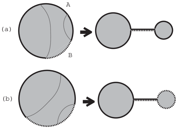
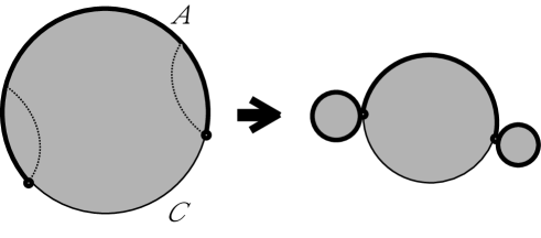
Figure 1: Due to the sticking of two different kinds of boundaries, the original loop splits into two loops with homogeneous matter configurations.

Figure 2: The original loop, composed of two different parts of a boundary, splits into two homogeneous loops and one heterogeneous loop.

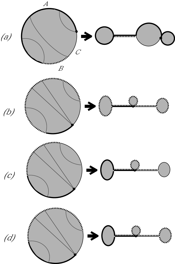
Figure 3: The original loop, composed of three different parts of a boundary, splits into three loops.

References

[1]
Harish-Chandra, Amer. J. Math. 79 (1957), 87.
C. Itzykson and J.-B. Zuber, J. Math. Phys. 21 (1980), 411.
[2]
V. A. Kazakov, Phys. Lett. A119 (1986), 140.
D. Boulatov and V. A. Kazakov, Phys. Lett. B186 (1987), 379.
[3]
M. Douglas, “The Two-matrix Model”,
Proceedings of Cargese Workshop, 1990.
T. Tada, Phys. Lett. B259 (1991), 442.
[4]
T. Tada and M. Yamaguchi, Phys. Lett. B250 (1990), 38.
[5]
J.-M. Daul, V. A. Kazakov and I. K. Kostov, Nucl. Phys. B409 (1993),
311.
[8]
F. Sugino and T. Yoneya, Phys. Rev. D53 (1996), 4448.
[9]
M. Anazawa, A. Ishikawa and H. Tanaka, Prog. Theor. Phys. 98 (1997),
457.
[10]
M. Anazawa, A. Ishikawa and H. Tanaka, Nucl. Phys. B514 (1998), 419.
[11]
M. Anazawa, Nucl. Phys. B501 (1997), 251.
[12]
E. Martinec, G. Moore and N. Seiberg,
Phys. Lett. B263 (1991), 190.
[13]
D. J. Gross and A. A. Migdal, Nucl. Phys. B340 (1990), 333.
M. Douglas and S. Shenker, Nucl. Phys. B335 (1990), 635.
E. Brezin and V. A. Kazakov, Phys. Lett. B236 (1990), 144.