Static dilaton solutions and singularities in six dimensional warped compactification with higher derivatives

Abstract

Static solutions with a bulk dilaton are derived in the context of six dimensional warped compactification. In the string frame, exponentially decreasing warp factors are identified with critical points of the low energy $\beta$-functions truncated at a given order in the string tension corrections. The stability of the critical points is discussed in the case of the first string tension correction. The singularity properties of the obtained solutions are analyzed and illustrative numerical examples are provided.

Preprint Number: UNIL-IPT-23 October 2000

I Formulation of the problem

Consider a $(4\,+2)-$dimensional space-time (consistent with four dimensional Poincaré invariance) of the form [1, 2]

$$ds^{2}=g_{\mu\nu}dx^{\mu}dx^{\nu}=\sigma(\rho)G_{ab}dx^{a}~{}dx^{b}-d\rho^{2}-\gamma(\rho)d\theta^{2},$$ (1.1)

where the (global) behavior of $\sigma(\rho)$ and $\gamma(\rho)$ should be determined by consistency with the appropriate equations of motion following, for instance, from the $(4\,+2)$-dimensional Einstein-Hilbert action . This type of compactification differs from ordinary Kaluza-Klein schemes [1, 2] (see also [3, 4]). The form of the line element given in Eq. (1.1) can be generalized to higher dimensions [5], although, for the present investigation, a six-dimensional metric will be considered.

Most of the studies dealing with six-dimensional warped compactification assume that the underlying theory of gravity is of Einstein-Hilbert type. Solutions with exponentially decreasing warp factors have been obtained in the presence of a bulk cosmological constant [6, 7] supplemented by either global [8, 9] or local [10] string-like defects (see also [11, 12]). The shape of the warp factor far and away from the core of the defect is always determined, in the quoted examples, according to the six-dimensional Einsten-Hilbert description. Six-dimensional warped compactifications represent a useful example also because they are a non-trivial generalization of warped compactifications in five dimensions [13].

Up to now the compatibility of warped compactification with theories different from the Einstein-Hilbert description have been analyzed mainly in the five-dimensional case. In particular the attention has been payed to gravity theories with higher derivatives [14, 15, 16]. In [17] the interesting problem of the compatibility of a five-dimensional compactification scheme with higher derivative gravity and dilaton field has been investigated. In [18] the simultaneous presence of higher dimensional hedgehogs and of higher derivatives gravity theories has been discussed in a seven-dimensional space-time.

The simultaneous presence of dilaton field and higher order curvature corrections is relevant for different reasons. There are two possible approaches to warped compactification schemes. In the first approach it is assumed, from the very beginning, that warped compactifications have nothing to do with string theory. The problem then reduces to the search of a suitable field theoretical model of higher dimensional (global or local) defects living along the transverse dimensions. A complementary approach is to postulate that warped compactifications are (somehow) connected to string theory. Even in this second approach, however, the dilaton field and the (possible) higher curvature terms (arising from the string tension corrections) are usually neglected [13]. The assumption that the dilaton field is strictly constant and that the string tension corrections are vanishing should be relaxed in order to investigate the (possible) interplay of warped compactification schemes with string models.

Five-dimensional warped compactifications have been studied in the context of generalized gravity theories with higher derivatives [14, 15, 16]. The inclusion of the dilaton field poses, however some problem. The main results concerning the interplay between five-dimensional warped compactifications and string motivated effective action can be summarized as follows [17]. If the dilaton is constant (but higher order curvature corrections are still present) five-dimensional warped compactifications are consistent with the effective action derived from the string amplitudes corrected to first order in the string tension.

If the dilaton is linear in the bulk coordinate warped compactification is not consistent with the presence of string tension corrections unless the conformal coupling between the dilaton and the string tension corrections is absent [17]. Interesting solutions interpolating between a naked singularity and a warped regime (for large bulk coordinate) have also been obtained. The purpose of the present investigation is to is to analyze the solutions of the metric (1.1) in the context of the string effective action [19, 20] with and without higher derivatives corrections [21, 22] (see also [23, 24]).

Up to now the compatibility of six-dimensional warped compactification with gravity theories inspired by string amplitudes has not been analyzed. In six-dimensional warped compactifications the transverse space is not flat (in contrast with the five-dimensional case). This observation implies on one hand that the internal space is larger and, on the other hand, that two warp factors are generically allowed. The tree-level solutions have more general singularity properties if compared to the five-dimensional case. These solutions are “Kasner-like” and they are the static analog of their time-dependent counterpart which is often discussed in cosmological solutions [25]. The inclusion of string tension corrections introduces also differences with respect to the five-dimensional case.

In six dimensions exponentially decreasing warp factors correspond to critical points of the $\beta$ functions computed at a given order in the string tension. Define, in fact, ${\cal H}=\partial_{\rho}(\ln\sigma)$ and ${\cal F}=\partial_{\rho}(\ln\gamma)$. By critical points we mean those (stable or unstable) solutions for which ${\cal H}$ and ${\cal F}$ are simultaneously constant and negative. The critical points of the system correspond to a static dilaton fields which either increases or decreases (linearly) for large $\rho$. Also the constant dilaton solution is possible. This situation should be contrasted with the five-dimensional case where only one warp factor is present.

The critical points are not always stable. If the initial conditions of the dilaton and of the warp factors are given around a given critical point (say for $\rho=\rho_{0}$) it can happen that for larger $\rho$ the compatibility with the $\beta$-functions will drive the solution away from the (original) critical point. In this case singularity may also be developed.

The present analysis is not meant to be exhaustive and suffers of two obvious limitations. In order to make an explicit calculation the effects of the first string tension correction has been studied. This is just an example since, when singularities are developed, all the string tension corrections should be included. The second point to be emphasized is that possible corrections in the dilaton coupling have also been neglected. This might be justified in some regimes of the solutions but it is not justified in more general terms. With these two warnings in mind the reported results should be understood more as possible indications than as a firm conclusion.

The present analysis has been performed in the string frame where the dilaton field is directly coupled both to the Einstein-Hilbert term and to the first string tension corrections. It is interesting to notice that singularity properties of a given solution may change from one frame to the other. A linearly increasing dilaton (in the string frame) results in curvature singularities in the Einstein frame (and vice-versa). The Einstein and the string frame are, however, physically equivalent. Suppose that the curvature invariants are regular in one frame and suppose that the dilaton is a smooth function of the bulk radius (interpolating, for instance, between two constant regimes). Then, the geometry looks regular in both frames enforcing the physical equivalence of the two descriptions.

In order to assess that six-dimensional warped compactification is fully consistent with the presence of the dilaton field and of string tension corrections some requirements should be, in our opinion, satisfied. The goal would be to obtain stable warped solutions with constant dilaton. Stable warped solutions means that the critical point of the low energy $\beta$ functions (truncated to first order in the $\alpha^{\prime}$ corrections) lead to exponentially decreasing warp factors. The constancy of the dilaton field $\phi$ implies the constancy of the coupling constant (i.e. $\exp{[\phi/2]}$) and this is a necessary (even though not sufficient) condition for the stability of the solutions. Notice that once the dilaton field and the string tension corrections are simultaneously present the problem of the singularity of the geometry cannot be disentangled from the problem of the dilaton relaxation.

The plan of the present investigation is then the following. In Section II the tree-level solution of the low energy string effective action will be studied. In Section III the first string tension correction will be included and the corresponding equations of motion will be derived. In Section IV the critical points of the obtained dynamical system will be analyzed. In Section V the stability of the critical points will be scrutinized and some numerical examples will be presented. Section VI contains some concluding remarks. In the Appendix useful technical results are reported.

II Tree-level solutions

If the curvature of the background is sufficiently small in units of the string length (denoted by $\lambda_{s}$) the massless modes of the string are weakly coupled and the dynamics can be described by the string effective action in six dimensions [19, 20]

$$S^{(0)}=\int d^{6}x\sqrt{-g}{\cal L}^{(0)}\equiv-\frac{1}{2\lambda_{s}^{4}}\int d^{6}x\sqrt{-g}e^{-\phi}\biggl{[}R+g^{\alpha\beta}\partial_{\alpha}\phi\partial_{\beta}\phi+\Lambda\biggr{]},$$ (2.1)

where $\phi$ is the dilaton field, $\lambda_{s}=\sqrt{\alpha^{\prime}}$ ($\alpha^{\prime}$ being the string tension). Eq. (2.1) is written in the string frame where the string scale is constant and the Planck scale depends upon the value of the dilaton coupling, i.e. $g(\phi)=e^{\phi/2}$. If the dilaton coupling is constant the the string frame coincides with Einstein frame. If, as in the present case, $\phi=\phi(\rho)$ the two frames are equivalent up to a conformal transformation. In the present paper the string frame will be used. In Eq. (2.1) the minimal field content (i.e. graviton and dilaton) has been assumed together with a bulk cosmological constant $\Lambda$. The effective action (2.1) is derived by requiring that the usual string scattering amplitudes are correctly reproduced to the lowest order in $\alpha^{\prime}$. The requirement that the equations of motion derived from Eq. (2.1) are satisfied in the metric (1.1) is equivalent to the requirement that the background is conformally invariant to the lowest order in $\alpha^{\prime}$. Notice that in eq. (2.1) the contribution of the antisymmetric tensor field has been neglected. This is justified within the spirit of the present analysis but this might not be justified in more general terms. We will come back on this point in the following Sections.

The equations of motion derived from the action of Eq. (2.1) can be written as

$$R-g^{\alpha\beta}\partial_{\alpha}\phi\partial_{\beta}\phi+2g^{\alpha\beta}\nabla_{\alpha}\nabla_{\beta}\phi+\Lambda=0,$$ (2.2)

$$R_{\mu\nu}-\frac{1}{2}g_{\mu\nu}R+\frac{1}{2}g_{\mu\nu}g^{\alpha\beta}\partial_{\alpha}\phi\partial_{\beta}\phi-g_{\mu\nu}g^{\alpha\beta}\nabla_{\alpha}\nabla_{\beta}\phi+\nabla_{\mu}\nabla_{\nu}\phi-\frac{\Lambda}{2}g_{\mu\nu}=0.$$ (2.3)

By now using the metric of Eq. (1.1) the explicit form of the $(a,\,a)$ and $(\theta,\,\theta)$ components of Eq. (2.3) will be

$$2\,{\Lambda}+{{\cal F}}^{2}+3\,{\cal F}\,{\cal H}+6\,{{\cal H}}^{2}+2\,{\cal F}^{\prime}+6\,{\cal H}^{\prime}-2\,{\cal F}\,{\phi}^{\prime}-6\,{\cal H}\,{\phi}^{\prime}+2\,{{\phi}^{\prime}}^{2}-4\,{\phi}^{\prime\prime}=0,$$ (2.4)

$$2\,{\Lambda}+10\,{{\cal H}}^{2}+8\,{\cal H}^{\prime}-8\,{\cal H}\,{\phi}^{\prime}+2\,{{\phi}^{\prime}}^{2}-4\,{\phi}^{\prime\prime}=0,$$ (2.5)

whereas the explicit form of the of Eq. (2.2) will be

$$-2\,{\Lambda}-{{\cal F}}^{2}-4\,{\cal F}\,{\cal H}-10\,{{\cal H}}^{2}-2\,{\cal F}^{\prime}-8\,{\cal H}^{\prime}+2\,{\cal F}\,{\phi}^{\prime}+8\,{\cal H}\,{\phi}^{\prime}-2\,{{\phi}^{\prime}}^{2}+4\,{\phi}^{\prime\prime}=0.$$ (2.6)

Notice that Eq. (2.2) has been multiplied by a factor two and Eq. (2.3) has been multiplied by a factor of four in order to get rid of rational coefficients. In deriving Eqs. (2.4)–(2.6) it has been assumed that, in Eq. (1.1) $G_{a\,b}\equiv\eta_{a\,b}$ where $\eta_{a\,b}$ is the Minkowski metric. Eqs. (2.4)–(2.6) admit exact solutions whose explicit form can be written as:

$$\sigma(\rho)=\tanh{\biggl{[}\frac{\sqrt{-\lambda}}{2}(\rho-\rho_{0})\biggr{]}}^{2\alpha},$$ (2.7)

$$\gamma(\rho)=\tanh{\biggl{[}\frac{\sqrt{-\lambda}}{2}(\rho-\rho_{0})\biggr{]}}^{2\beta},$$ (2.8)

$$e^{\phi(\rho)}=\frac{1}{2}\biggl{\{}\sinh{\biggl{[}\frac{\sqrt{-\Lambda}}{2}(\rho-\rho_{0})\biggr{]}}\biggr{\}}^{4\alpha+\beta-1}\biggl{\{}\cosh{\biggl{[}\frac{\sqrt{-\Lambda}}{2}(\rho-\rho_{0})\biggr{]}}\biggr{\}}^{-4\alpha-\beta-1},$$ (2.9)

The exponents $\alpha$ and $\beta$ satisfy the condition $4\alpha^{2}+\beta^{2}=1$. Eqs. (2.7)–(2.9) lead to a physical singularity for $\rho\rightarrow\rho_{0}$. All curvature invariants associated with the metric (1.1) for the specific solution given in Eqs. (2.7)–(2.9) diverge for $\rho\rightarrow\rho_{0}$ (see Appendix A for the details). If $\alpha=\beta$ the Weyl invariant vanishes but the other invariants are still singular.

If $\Lambda\rightarrow 0$, Eqs. (2.4)–(2.6) are solved by

$$\sigma(\rho)=(\rho-\rho_{0})^{2\alpha},$$ (2.10)

$$\gamma(\rho)=(\rho-\rho_{0})^{2\beta},$$ (2.11)

$$e^{\phi(\rho)}=(\rho-\rho_{0})^{-1+4\alpha+\beta},$$ (2.12)

provided $4\alpha^{2}+\beta^{2}=1$. Eqs. (2.7)–(2.9) and (2.10)–(2.12) are Kasner-like solutions whose time-dependent analog has been widely exploited in the context of string cosmological solutions [25].

In the case of $\Lambda<0$ this system of equation has a further non trivial solution which is given by ${\cal H}$, ${\cal F}$ and $\phi^{\prime}$ all constant. In this case the solution of the previous system of equations is given by

$$4\Lambda+4{\cal H}^{2}+{\cal F}^{2}=0,\,\,\,\,2\phi^{\prime}=4{\cal H}+{\cal F}.$$ (2.13)

In the particular case where $\sigma(\rho)\propto\gamma(\rho)$ ( i.e. ${\cal H}={\cal F}$), the solution is ${\cal H}=-\sqrt{-4\Lambda/5}$. As we will discuss in Section IV this solution is not always stable.

The presence of curvature singularities in the tree-level solutions obtained in Eqs. (2.7)–(2.9) and (2.10)–(2.11) suggests that there are physical regimes where the curvature of the geometry will approach the string curvature scale. In this situation higher order (curvature) corrections may play a role in stabilizing the solution and should be considered. The following part of this investigation will then deal with the inclusion of the first $\alpha^{\prime}$ correction. This analysis is of course not conclusive per se since also higher orders in $\alpha^{\prime}$ should be considered as it has been argued in Section I.

III First order $\alpha^{\prime}$ corrections

Consider now the first $\alpha^{\prime}$ correction to the action $S^{(0)}$ presented in Eq. (2.1). The full action is, in this case [21]

$$S=S^{(0)}\,+\,S^{(1)}=-\frac{1}{2\lambda_{s}^{4}}\int\,d^{6}x\,\sqrt{-g}\,e^{-\phi}\,\biggl{[}R\,+\,g^{\alpha\beta}\partial_{\alpha}\phi\partial_{\beta}\phi\,+\,\Lambda-\epsilon\,R_{\mu\nu\alpha\beta}\,R^{\mu\nu\alpha\beta}\biggr{]},$$ (3.1)

where $\epsilon=k\alpha^{\prime}/4$ and the constant $k$ takes different values depending upon the specific theory ( $k=1$ for the bosonic theory, $k=1/2$ for the heterotic theory). Notice that the assumption made in the previous Section (concerning the absence of antisymmetric tensor field) reflects in the fact that the first $\alpha^{\prime}$ correction appears precisely in the form reported in eq. (3.1). If the antisymmetric tensor field would not be vanishing the first string tension correction to the tree-level action would look like [21]

$$-\epsilon\biggl{(}R_{\mu\nu\alpha\beta}R^{\mu\nu\alpha\beta}-\frac{1}{2}R^{\mu\nu\alpha\beta}H_{\alpha\beta\lambda}H^{\lambda}_{\,\mu\nu}\biggr{.}$$ (3.2)

$$+\biggl{.}\frac{1}{24}H_{\mu\nu\lambda}H^{\nu}_{\,\rho\alpha}H^{\rho\sigma\lambda}H_{\sigma}^{\,\mu\alpha}-\frac{1}{8}H_{\mu\alpha\beta}H_{\nu}^{\,\alpha\beta}H^{\mu\rho\sigma}H^{\nu}_{\,\rho\sigma}\biggr{)}+{\cal O}(\epsilon^{2})$$ (3.3)

where $H_{\mu\nu\alpha}$ is the antisymmetric tensor field strength. If $H_{\mu\nu\alpha}$ vanishes identically the only correction to the tree-level action is the one coming from the first term of Eq. (3.3). However, if $H_{\mu\nu\alpha}\neq 0$, the situation changes qualitatively. We leave this intriguing issue for future investigations.

The fields appearing in the action (3.1) can be redefined (preserving the perturbative string amplitudes) [21, 23]. In order to discuss actual solutions it is useful to perform a field redefinition (keeping the $\sigma$ model parameterization of the action) that eliminates terms with higher than second derivatives from the effective equations of motion [21, 22] (see also [23, 24]). In six dimensions the field redefinition can be written as

$$\overline{g}_{\mu\nu}=g_{\mu\nu}+16\epsilon\biggl{[}R_{\mu\nu}\,-\,\partial_{\mu}\phi\partial_{\nu}\phi\,+\,g_{\mu\nu}g^{\alpha\beta}\partial_{\alpha}\phi\partial_{\beta}\phi\biggr{]},$$ (3.4)

$$\overline{\phi}=\phi+\epsilon\,\biggl{[}R+(3+2n)g^{\alpha\beta}g^{\rho\sigma}\partial_{\alpha}\phi\,\partial_{\beta}\phi\,\partial_{\rho}\phi\,\partial_{\sigma}\phi\,\biggr{]},$$ (3.5)

where $n$ (the number of transverse dimensions) is equal to 2 in the case of the present analysis. Dropping the bar in the redefined fields the action reads :

$$S=-\frac{1}{2\lambda_{s}^{4}}\int d^{6}x\sqrt{-g}e^{-\phi}\biggl{[}R+g^{\alpha\beta}\partial_{\alpha}\phi\partial_{\beta}\phi+\Lambda-\epsilon\biggl{(}R_{\rm EGB}^{2}-g^{\alpha\beta}g^{\rho\sigma}\partial_{\alpha}\phi\partial_{\beta}\phi\partial_{\rho}\phi\partial_{\sigma}\phi\biggl{)}\biggr{]},$$ (3.6)

where

$$R^{2}_{\rm EGB}=R_{\mu\nu\alpha\beta}R^{\mu\nu\alpha\beta}-4R_{\mu\nu}R^{\mu\nu}+R^{2},$$ (3.7)

is the Euler-Gauss-Bonnet invariant (which coincides, in four space-time dimensions, with the Euler invariant ). The equations of motion can be easily derived by varying the action (3.6) with respect to the metric and with respect to the dilaton field (see Appendix B for details). The result is that

$$2\,{\Lambda}+{{\cal F}}^{2}+3\,{\cal F}\,{\cal H}+6\,{{\cal H}}^{2}+2\,{\cal F}^{\prime}+6\,{\cal H}^{\prime}-2\,{\cal F}\,{\phi}^{\prime}-6\,{\cal H}\,{\phi}^{\prime}+2\,{{\phi}^{\prime}}^{2}-4\,{\phi}^{\prime\prime}$$ (3.8)

$$+\epsilon\,\bigl{[}-3\,{{\cal F}}^{2}\,{{\cal H}}^{2}-9\,{\cal F}\,{{\cal H}}^{3}-3\,{{\cal H}}^{4}-6\,{{\cal H}}^{2}\,{\cal F}^{\prime}-12\,{\cal F}\,{\cal H}\,{\cal H}^{\prime}-6\,{{\cal H}}^{2}\,{\cal H}^{\prime}+\bigr{.}$$ (3.9)

$$\bigl{.}6\,{{\cal F}}^{2}\,{\cal H}\,{\phi}^{\prime}+24\,{\cal F}\,{{\cal H}}^{2}\,{\phi}^{\prime}+18\,{{\cal H}}^{3}\,{\phi}^{\prime}+12\,{\cal H}\,{\cal F}^{\prime}\,{\phi}^{\prime}\bigr{.}$$ (3.10)

$$\bigr{.}+12\,{\cal F}\,{\cal H}^{\prime}\,{\phi}^{\prime}+24\,{\cal H}\,{\cal H}^{\prime}\,{\phi}^{\prime}-12\,{\cal F}\,{\cal H}\,{{\phi}^{\prime}}^{2}-12\,{{\cal H}}^{2}\,{{\phi}^{\prime}}^{2}\bigr{.}+$$ (3.11)

$$\bigl{.}2\,{{\phi}^{\prime}}^{4}+12\,{\cal F}\,{\cal H}\,{\phi}^{\prime\prime}+12\,{{\cal H}}^{2}\,{\phi}^{\prime\prime}\bigr{]}=0,$$ (3.12)

$$2\,{\Lambda}+10\,{{\cal H}}^{2}+8\,{\cal H}^{\prime}-8\,{\cal H}\,{\phi}^{\prime}+2\,{{\phi}^{\prime}}^{2}-4\,{\phi}^{\prime\prime}+$$ (3.13)

$$\epsilon\,\bigl{[}-15\,{{\cal H}}^{4}-24\,{{\cal H}}^{2}\,{\cal H}^{\prime}+48\,{{\cal H}}^{3}\,{\phi}^{\prime}+48\,{\cal H}\,{\cal H}^{\prime}\,{\phi}^{\prime}-24\,{{\cal H}}^{2}\,{{\phi}^{\prime}}^{2}+\bigr{.}$$ (3.14)

$$\bigl{.}2\,{{\phi}^{\prime}}^{4}+24\,{{\cal H}}^{2}\,{\phi}^{\prime\prime}\bigr{]}=0,$$ (3.15)

$$-2\,{\Lambda}-{{\cal F}}^{2}-4\,{\cal F}\,{\cal H}-10\,{{\cal H}}^{2}-2\,{\cal F}^{\prime}-8\,{\cal H}^{\prime}+2\,{\cal F}\,{\phi}^{\prime}+8\,{\cal H}\,{\phi}^{\prime}-2\,{{\phi}^{\prime}}^{2}+4\,{\phi}^{\prime\prime}$$ (3.16)

$$+\epsilon\,\bigl{[}6\,{{\cal F}}^{2}\,{{\cal H}}^{2}+24\,{\cal F}\,{{\cal H}}^{3}+15\,{{\cal H}}^{4}+12\,{{\cal H}}^{2}\,{\cal F}^{\prime}+24\,{\cal F}\,{\cal H}\,{\cal H}^{\prime}+24\,{{\cal H}}^{2}\,{\cal H}^{\prime}\bigr{.}$$ (3.17)

$$\bigl{.}-4\,{\cal F}\,{{\phi}^{\prime}}^{3}-16\,{\cal H}\,{{\phi}^{\prime}}^{3}+6\,{{\phi}^{\prime}}^{4}-24\,{{\phi}^{\prime}}^{2}\,{\phi}^{\prime\prime}\bigr{]}=0.$$ (3.18)

In the limit $\epsilon\rightarrow 0$ the equations derived in Section II are recovered. Eqs. (3.12)–(3.18) can be studied in order to investigate two separate issues. The first one is the existence of critical points leading to exponentially decreasing warp factors. The second issue would be to analyze the stability of these critical points. Indeed, in the solutions given in Eqs. (2.7)–(2.9) a singularity is developed. This result is based, however, on the tree-level action. If the first $\alpha^{\prime}$ correction is included this feature might change. Moreover, if $\Lambda=0$ there are no warped solutions at tree-level. These solutions might emerge, however, when $\alpha^{\prime}$ corrections are included. For instance, the “Kasner-like” branch of the solution might be analytically connected to a “warped” regime where ${\cal H}$ and ${\cal F}$ are both constant and negative. These questions will be the subject of the following Section.

In closing this section we want to recall that in [29] it has been claimed that (five-dimensional) warped compactifications cannot be obtained in the low energy supergravities coming from string theory. In this context it has also been suggested that higher order corrections to the Einstenian action might help in evading this conclusion. In the following we will explore an analogous possibility.

IV Dynamical system and critical points

Defining

$$x(\rho)\equiv{\cal H}(\rho),~{}~{}~{}~{}y(\rho)\equiv{\cal F}(\rho),~{}~{}~{}~{}~{}~{}z(\rho)\equiv\phi^{\prime}(\rho),$$ (4.1)

Eqs. (3.12)–(3.18) can be written as

$$p_{x}(\rho)\,x^{\prime}+p_{y}(\rho)\,y^{\prime}+p_{z}(\rho)\,z^{\prime}+p_{0}(\rho)=0,$$ (4.2)

$$q_{x}(\rho)\,x^{\prime}+q_{z}(\rho)z^{\prime}+q_{0}(\rho)=0,$$ (4.3)

$$w_{x}(\rho)\,x^{\prime}+w_{y}(\rho)\,y^{\prime}+w_{z}(\rho)\,z^{\prime}+w_{0}(\rho)=0.$$ (4.4)

The $p$ are

$$p_{x}(\rho)=6\{1-\epsilon[x(x+2y)-2z(y+2x)]\},\,\,\,\,$$ (4.5)

$$p_{y}(\rho)=2[1-3\epsilon x(x-2z)],\,\,\,\,\,p_{z}(\rho)=-4[1-3\epsilon x(x+y)],$$ (4.6)

$$p_{0}(\rho)=2\Lambda+y(y+3x)+6x^{2}-2z(y+3x)+2z^{2}$$ (4.7)

$$+\epsilon[-3x^{2}(y^{2}+3xy+x^{2})+6x(x+y)(y+3x)z-12x(x+y)z^{2}+2z^{4}],$$ (4.8)

whereas the $q$ are

$$q_{x}(\rho)=8[1-3\epsilon x(x-2z)],\,\,\,\,\,q_{z}(\rho)=-4(1-6\epsilon x^{2}),$$ (4.9)

$$q_{0}(\rho)=2\Lambda+2(z^{2}-4xz+5x^{2})+\epsilon[-15x^{4}+48x^{3}z-24x^{2}z^{2}+2z^{4}],$$ (4.10)

and finally the $w$ are

$$w_{x}(\rho)=-8[1-3\epsilon x(x+y)],$$ (4.11)

$$w_{y}(\rho)=-2[1-6\epsilon x^{2}],\,\,\,\,\,w_{z}(\rho)=4(1-6\epsilon z^{2}),$$ (4.12)

$$w_{0}(\rho)=-2\Lambda-(y^{2}+4xy+10x^{2})+2(y+4x)z-2z^{2}$$ (4.13)

$$+\epsilon[3x^{2}(2y^{2}+8xy+5x^{2})-4(y+4x)z^{3}+6z^{4}].$$ (4.14)

Eqs. (4.2)–(4.4) can be analyzed both analytically and numerically. Interesting analytical conclusions can be obtained, for instance, in the case $x(\rho)=y(\rho)$. In the remaining part of the present Section the stability of the system will be analyzed. Physical (i.e. curvature) singularities will be investigated. The logic will be, in short, the following. The critical points will be firstly studied analytically. Indeed, it happens that, in spite of the apparent complications of the system, there are limits in which analytical expressions can be given. Numerical examples will be given for the other cases which are not solvable analytically. The examples studied in the present Session will be exploited in Section V for some explicit numerical solutions.

The critical points of the system derived in Eqs. (4.2)–(4.4) are defined to be the one for which [30]

$$x^{\prime}(\rho)=0,\,\,\,y^{\prime}(\rho)=0,\,\,\,z^{\prime}(\rho)=0.$$ (4.15)

The critical points interesting for warped compactifications are the ones for which $x(\rho)$ and $y(\rho)$ are not only constant but also negative. These points lead, for large $\rho$, to exponentially decreasing warp factors in the six-dimensional metric.

In the case of Eq. (4.15) the solution of the system reduces to a system of three algebraic equations in the unknowns $(x,y,z)$. The three equations of the system are simply given by the conditions

$$p_{0}(\rho)=0,\,\,\,\,q_{0}(\rho)=0,\,\,\,\,w_{0}(\rho)=0,$$ (4.16)

namely,

$$2\Lambda+y(y+3x)+6x^{2}-2z(y+3x)+2z^{2}$$ (4.17)

$$+\epsilon[-3x^{2}(y^{2}+3xy+x^{2})+6x(x+y)(y+3x)z-12x(x+y)z^{2}+2z^{4}]=0,$$ (4.18)

$$2\Lambda+2(z^{2}-4xz+5x^{2})+\epsilon[-15x^{4}+48x^{3}z-24x^{2}z^{2}+2z^{4}]=0,$$ (4.19)

$$-2\Lambda-(y^{2}+4xy+10x^{2})+2(y+4x)z-2z^{2}$$ (4.20)

$$+\epsilon[3x^{2}(2y^{2}+8xy+5x^{2})-4(y+4x)z^{3}+6z^{4}]=0.$$ (4.21)

By summing up, respectively, Eqs. (4.18) and (4.19) with Eq. (4.21) the following two algebraic conditions are obtained:

$$(4x+y-2z)[3\epsilon x^{3}-4\epsilon z^{3}+3\epsilon x^{2}(y+2z)+x(-1+6\epsilon yz)]=0,$$ (4.22)

$$(4x+y-2z)[y(-1+6\epsilon x^{2})-4\epsilon z(z^{2}-3x^{2})]=0.$$ (4.23)

A third algebraic relations is obtained by subtracting Eq. (4.19) from Eq. (4.18):

$$(x-y)(4x+y-2z)[-1+3\epsilon x(x-2z)]=0.$$ (4.24)

If $x=y$ Eqs. (4.18)–(4.21) are solved provided

$$x=y,\,\,\,\,\,z=\frac{4x+y}{2},\,\,\,\,\,$$ (4.25)

$$16\Lambda+20x^{2}+265\epsilon x^{4}=0,$$ (4.26)

and an explicit solution corresponding to the critical points of the system (4.18)–(4.21) can then be written as

$$\sigma(\rho)=e^{\bigl{(}\frac{\rho}{\rho_{1}}\bigr{)}},\,\,\,\,\,\gamma(\rho)=\gamma_{0}\sigma(\rho)$$ (4.27)

$$\phi(\rho)=\frac{5}{2}\bigl{(}\frac{\rho}{\rho_{1}}\bigr{)}+\phi_{0}$$ (4.28)

where $\gamma_{0}$ and $\phi_{0}$ are integration constants and where

$$\rho_{1}=\pm\sqrt{-\frac{5}{8\Lambda}}\sqrt{1\mp\sqrt{1-\frac{212}{5}\Lambda\epsilon}}$$ (4.29)

is obtained from the real roots of the algebraic equation appearing in Eq. (4.26). A priori, depending upon the sign of $\Lambda$ and upon the relative weight of $\Lambda\epsilon$, $\rho_{1}$ can be either positive or negative.

The solution derived in Eqs. (4.26) does not exhaust the possible critical points even in the case $x=y$. Consider, in fact, Eqs. (4.18)–(4.21) in the case $x=y$ but with $z\neq 5\,x/2$. In this case Eq. (4.18) and Eq. (4.19) lead to the same algebraic equation

$$2\,\Lambda+2\,\left(5\,x^{2}-4\,x\,z+z^{2}\right)+\epsilon\,\left(-15\,x^{4}+48\,x^{3}\,z-24\,x^{2}\,z^{2}+2\,z^{4}\right)=0,$$ (4.30)

whereas Eq. (4.21) leads to

$$-2\,\Lambda-15\,x^{2}+10\,x\,z-2\,z^{2}+\epsilon\,\left(45\,x^{4}-20\,x\,z^{3}+6\,z^{4}\right)=0.$$ (4.31)

Eqs. (4.30)–(4.31) cannot be further simplified and the best one can do is to solve them once the values of $\epsilon$ and $\Lambda$ are specified. If $\Lambda=-1$ and $\epsilon=0.1$ the real roots of the system of Eqs. (4.30)–(4.31) are given by:

$$(x_{1},\,z_{1})=\pm(0.6974,\,1.7436),\,\,\,\,\,(x_{2},\,z_{2})=(\pm 1.3775,\mp 2.3429),$$ (4.32)

$$(x_{3},\,z_{3})=(\pm 0.1338,\,\mp 0.7176),\,\,\,(x_{4},\,z_{4})=(\pm 1.9645,\,\mp 0.5744).$$ (4.33)

On top of the real roots reported in Eqs. (4.32)–(4.33) there are also imaginary roots which are not relevant for the present discussion. The first pair of roots in Eq. (4.32) can also be obtained from Eq. (4.26). Notice, also, that $(x_{1},\,z_{1})$ is the only root where the $z$ and $x$ can be simultaneously negative (when the minus sign is chosen). The other roots are such that $x$ and $z$ always have opposite signs. The same discussion can be repeated for different values of $\Lambda$ and $\epsilon$. For instance, if $\Lambda=-2$ and $\epsilon=0.1$ the real roots of Eqs. (4.30)–(4.31) are

$$(x_{1},\,z_{1})=\pm(0.8857,\,2.2143),\,\,\,(x_{2},z_{2})=(\pm 1.3490,\,\mp 2.3077),$$ (4.34)

$$(x_{3},\,z_{3})=\pm(1.0275,\,1.6067),\,\,\,(x_{4},z_{4})=(\pm 0.2455,\,\mp 0.9111),$$ (4.35)

$$(x_{5},\,x_{5})=\pm(0.8563,0.7023),\,\,\,(x_{6},z_{6})=(\pm 1.9285,\,\mp 0.5468).$$ (4.36)

If $x\neq y$ and, simultaneously, $z\neq(4x+y)/2$ the system of Eqs. (4.18)–(4.21) can still be solved. From Eqs. (4.23) and (4.24) an ansatz for the algebraic solution can be written as

$$z=\frac{3\epsilon x^{2}-1}{6\epsilon x},$$ (4.37)

$$y=\frac{1-9\epsilon x^{2}-81\epsilon^{2}x^{4}+297\epsilon^{3}x^{6}}{54\epsilon^{2}x^{3}-324\epsilon^{3}x^{5}}.$$ (4.38)

By inserting this ansatz back into Eqs. (4.18)–(4.21) the same equation for $x$ is obtained from all three equations of the system, namely,

$$2\,\Lambda+\frac{5}{12\,\epsilon}+\frac{1}{648\,\epsilon^{3}\,x^{4}}+\frac{1}{27\,\epsilon^{2}\,x^{2}}+\frac{7\,x^{2}}{3}+\frac{25\,\epsilon\,x^{4}}{8}=0.$$ (4.39)

Thus, the critical points of the system of Eqs. (4.18)–(4.21) [in the case $x\neq y$, $x\neq 0$ and $z\neq(4x+y)/2$] are given by

$$z=\frac{3\epsilon x^{2}-1}{6\epsilon x},\,\,\,\,y=\frac{1-9\epsilon x^{2}-81\epsilon^{2}x^{4}+297\epsilon^{3}x^{6}}{54\epsilon^{2}x^{3}-324\epsilon^{3}x^{5}},$$ (4.40)

$$P(x,\Lambda,\epsilon)=\frac{1}{648\,\epsilon^{3}}+\frac{x^{2}}{27\,\epsilon^{2}}+\left(2\,\Lambda+\frac{5}{12\,\epsilon}\right)\,x^{4}+\frac{7\,x^{6}}{3}+\frac{25\,\epsilon\,x^{8}}{8}=0.$$ (4.41)

Eq. (4.41) should be solved for real values of $x$. The critical points corresponding to negative (and real) roots of Eq. (4.41) lead to exponentially decaying $\sigma(\rho)$. Once the real roots of Eqs. (4.41) are obtained, Eqs. (4.40) will give the wanted values of $y$ and $z$.

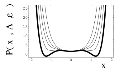
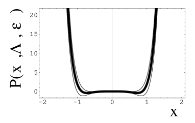
FIG. 1.: $P(x,\Lambda,\epsilon)$ appearing in Eq. (4.41) is plotted in the case of $\epsilon=0.1$ (left) and $\epsilon=1$ (right) and for different values of $\Lambda$. In the left plot the thick line corresponds to the case $\Lambda=-6$ where $P(x,\Lambda,\epsilon)$ has real roots. The other thin lines (from bottom to top) correspond, respectively, to $\Lambda=-5,-4,-3,-1$. In the right plot the thick curve correspond to the case $\Lambda=-2$ and the two thin lines correspond, from bottom to to top, to $\Lambda=-3$ and $\Lambda=-1$.

Eq. (4.41) does not always have real roots. In Fig. 1 $P(x,\Lambda,\epsilon)$ is reported as a function of $x$ and for different values of $\Lambda$ and $\epsilon$. The specific values are only representative and will be used in specific numerical solutions later on. For instance, it can be argued from Fig. 1 that if $\epsilon=0.1$ real roots of Eq. (4.41) start appearing for $\Lambda<-6$.

V Stability of the critical points, singularities and numerical examples

If $x(\rho)\equiv y(\rho)$ [i.e. $\gamma(\rho)=\gamma_{0}\sigma(\rho)$], Eqs. (4.2)–(4.3) lead exactly to the same equation so that the only two independent equations obtained in this case are:

$$a_{x}(\rho)\,x^{\prime}+a_{z}(\rho)\,z^{\prime}+a_{0}(\rho)=0,$$ (5.1)

$$b_{x}(\rho)\,x^{\prime}+b_{z}(\rho)\,z^{\prime}+b_{0}(\rho)=0.$$ (5.2)

where

$$a_{x}(\rho)=8[1-3\epsilon x(x-2z)],\,\,\,\,a_{z}(\rho)=-4(1-6\epsilon x^{2}),$$ (5.3)

$$b_{x}(\rho)=-10(1-6\epsilon x^{2}),\,\,\,\,\,\,b_{z}(\rho)=4(1-6\epsilon z^{2}),$$ (5.4)

and

$$a_{0}(\rho)=[2\Lambda+10x^{2}-8xz+2z^{2}+\epsilon(-15x^{4}+48x^{3}z-24x^{2}z^{2}+2z^{4})],$$ (5.5)

$$b_{0}(\rho)=[-2\Lambda-15x^{2}+10xz-2z^{2}+\epsilon(45x^{4}-20xz^{3}+6z^{4})].$$ (5.6)

Notice that the If $\Lambda=0$, from Eq. (4.26) $\rho_{1}$ becomes purely imaginary. If $\Lambda<0$ and if $\rho_{1}$ has to be real there are two relevant critical points, namely

$$\rho_{1}=\pm\sqrt{\frac{5}{8\Lambda_{-}}}\sqrt{1+\sqrt{1+\frac{212}{5}\Lambda_{-}\epsilon}},$$ (5.7)

where, for convenience, $\Lambda=-\Lambda_{-}$ (with $\Lambda_{-}>0$). In order to have a warped compactification scheme, $\rho_{1}<0$ and, therefore, only one critical point satisfies this requirement.

If, as a warm-up, $\epsilon\rightarrow 0$ a critical point of the system is indeed given by Eq. (2.13). The tree-level critical point is not stable. Indeed, in the case $\epsilon=0$ Eqs. (5.2) can be written as

$$x^{\prime}=f_{x}(x,z),\,\,\,\,\,z^{\prime}=f_{z}(x,z),$$ (5.8)

where

$$f_{x}(x,z)=xz-\frac{5}{2}x^{2},$$ (5.9)

$$f_{z}(x,z)=\frac{\Lambda}{2}-\frac{5}{2}x^{2}+\frac{z^{2}}{2}.$$ (5.10)

The partial derivatives of $f_{x}(x,z)$ and $f_{z}(x,z)$ (i.e. $\partial_{x}f_{x}$, $\partial_{z}f_{x}$ and $\partial_{x}f_{z}$, $\partial_{z}f_{z}$) define a matrix whose entries should be evaluated in the critical points, corresponding, in the present case, to $z=(5/2)x$, $x=-\sqrt{4\Lambda_{-}/5}$. The eigenvalues of this matrix are simply given by $\delta_{1,\,2}=\mp\sqrt{5\Lambda_{-}/4}$. Therefore, the tree-level critical point is an unstable node since the eigenvalues are both real and with opposite signs (i.e. $\delta_{1}\delta_{2}<0$).

Suppose now to turn on the first $\alpha^{\prime}$ correction. Then $\epsilon\neq 0$. In this case the tree-level discussion can be repeated. If $\epsilon\neq 0$ the dynamical system will now become [always in the case $x(\rho)=y(\rho)$]

$$x^{\prime}=g_{x}(x,z),\,\,\,\,\,z^{\prime}=g_{z}(x,z),$$ (5.11)

where now, from eq. (5.2)

$$g_{x}(x,z)=\frac{a_{z}b_{0}-a_{0}b_{z}}{b_{x}a_{z}-a_{x}b_{z}},$$ (5.12)

$$g_{z}(x,z)=\frac{a_{x}b_{0}-a_{0}b_{x}}{b_{x}a_{z}-a_{x}b_{z}}.$$ (5.13)

In analogy with the previous case the matrix of the derivatives can be constructed. The two eigenvalues of such a matrix are complex conjugate numbers of the form

$$W_{1,\,2}=\sqrt{\Lambda_{-}}[\mu(k)\pm i~{}\nu(k)].$$ (5.14)

where $k=\Lambda_{-}\epsilon$ and the subscripts $1$ and $2$ correspond, respectively, to the plus and minus signs. The expressions are quite cumbersome so that they are reported in the Appendix C. In order to determine the stability of the system the sign of $\mu(k)$ is crucial. It turns out, from a numerical analysis of Eqs. (C.1)–(C.2), that

$$\mu(k)>0,\,\,\,\,{\rm for}\,\,\,k=\Lambda_{-}\epsilon>0.65,$$ (5.15)

$$\mu(k)<0,\,\,\,\,{\rm for}\,\,\,k=\Lambda_{-}\epsilon<0.65.$$ (5.16)

Thus, for $\Lambda_{-}\epsilon>0.65$ there is an unstable spiral point whereas for $\Lambda_{-}\epsilon<0.65$ there is a stable spiral point [30].

In closing this session an interesting solution can be mentioned. In the case $\Lambda=0$ and $z=0$ (constant dilaton case) the relevant equations can be written as :

$$6[1-\epsilon\,x(x+2y)]x^{\prime}+2[1-3\epsilon x^{2}]y^{\prime}+2\Lambda+6x^{2}$$ (5.17)

$$+y(y+3x)-3\epsilon x^{2}(y^{2}+3xy+x^{2})=0,$$ (5.18)

$$8(1-3\epsilon x^{2})x^{\prime}+2\Lambda+10x^{2}-15\epsilon x^{4}=0.$$ (5.19)

The critical point of the system can be obtained also in this case and it corresponds to $x_{c}=y_{c}=-\sqrt{2/(3\,\epsilon)}$. The system can then be written in its canonical form, namely, $x^{\prime}=F_{x}(x,y)$ and $y^{\prime}=F_{y}(x,y)$. The eigenvalues of the matrix of the derivatives evaluated in $(x_{c},\,y_{c})$ are, respectively, $\delta_{1}=5/\sqrt{6\epsilon}$ and $\delta_{2}=5(3\epsilon-1)/\sqrt{6\epsilon}$. Notice that $\delta_{1}\delta_{2}=[25(3\epsilon-1)]/(6\epsilon)$. This means that the critical point is a saddle point for $\epsilon<1/3$ and an unstable node for $\epsilon>1/3$ [30]. This solution, even though interesting, is only illustrative : the presence of the inverse coupling in the critical point clearly points towards non-perturbative effects which should be properly discussed by adding higher orders in $\alpha^{\prime}$.

A Numerical examples

A Kasner-like branch can be analytically connected to a constant curvature solution where $x_{0}<0$ and the dilaton is linearly decreasing ($z_{0}<0$). Suppose that $\Lambda=-1$ and $\epsilon=0.1$. Then, we can see that there exist a solution connecting the Kasner-like regime to a critical point given by Eqs. (4.26) and (4.32).

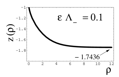
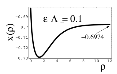
FIG. 2.: A numerical solution of the system given in Eq. (5.2) is reported in the case $\Lambda=-1$ and $\epsilon=0.1$. The solution interpolates between the Kasner-like regime (for $\rho\rightarrow 0$) and the critical point given by the solution of Eq. (4.26) which is explicitly given (for the chosen values of $\Lambda$ and $\epsilon$) by the first pair of roots appearing in Eq. (4.32).

The numerical result is reported in Fig. 2. For large $\rho$ the solution matches exactly the critical point which can be obtained (with $\Lambda=-1$ and $\epsilon=0.1$) from Eq. (4.26) and which are reported in the first pair of roots in Eq. (4.32).

If the initial conditions are not given in the Kasner-like regime but in the vicinity of a critical point there are various possibilities. It can happen that the system is driven (smoothly) towards another critical point or it can happen that a singularity is reached.

Suppose that the initial conditions for the numerical integration of the system of Eq. (5.2) are given in in $\rho\sim 0$ requiring that $x(0)<0$ and $z(0)<0$ according to the solution of Eqs. (4.26). In this case, the system seats exactly on a critical point whose properties have been previously analyzed. In the case $\Lambda=-1$ and $\epsilon=0.1$ the initial conditions are fixed for $x(0)\equiv x_{1}$ and $z(0)\equiv z_{1}$ where $(x_{1},\,z_{1})$ are given by Eq. (4.32). In this case the system evolves towards a different critical point, namely it happens that $x(\infty)\rightarrow x_{3}$ and $z(\infty)\rightarrow z_{3}$ where $(x_{3},\,z_{3})$ are given by Eq. (4.33). This conclusion can be obtained by direct numerical integration. In Fig. 3 the numerical integration is reported for the mentioned initial conditions. It can be seen that $x(50)=0.133$ and $z(50)=-0.7176$ which, indeed, coincide with $x_{3}$ and $z_{3}$ within the numerical accuracy of the present analysis.

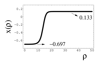
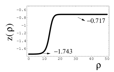
FIG. 3.: The numerical integration of Eqs. (5.2) is reported in the case $\Lambda=-1$ and $\epsilon=0.1$. The critical points in this specific case were given explicitly in Eqs. (4.32)–(4.33). Initial conditions are given in one of them, namely $(x_{1},\,z_{1})$.

The singularity structure of the curvature invariants can be appreciated by analyzing the behavior of

$$I_{1}(\rho)=R_{\mu\nu\alpha\beta}R^{\mu\nu\alpha\beta},\,\,\,\,I_{2}(\rho)=C_{\mu\nu\alpha\beta}C^{\mu\nu\alpha\beta}$$ (5.20)

$$I_{3}(\rho)=R,\,\,\,\ I_{4}(\rho)=R_{\mu\nu}R^{\mu\nu}$$ (5.21)

whose general form is reported, for the metric (1.1), in Appendix C. Notice that if $x=y$, as in the example of Fig. 3, the Weyl invariant vanishes.

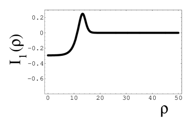
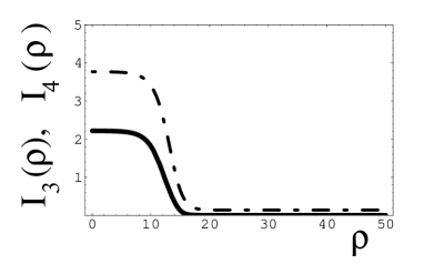
FIG. 4.: In the case of $\Lambda=-1$ and $\epsilon=0.1$ the curvature invariants corresponding to the solution reported in Fig. 3 are reported. The Riemann invariant appears in the left plot with full thick line. At the right the Ricci invariant is reported with dot-dashed line. The scalar curvature is reported (always in the right plot) with the full (thick) line.

Suppose now that $\Lambda=-2$ and $\epsilon=0.1$. The critical points are given by Eqs. (4.34)–(4.36). The initial conditions imposed in $\rho=0$ will be such that $x(0)<0$ and $z(0)<0$ as in the previous numerical example. Requiring, from Eq. (4.34), $x(0)=x_{1}$ and $z(0)=z_{1}$ the numerical integration leads to a divergence for large $\rho$. In this specific case, the singularity occurs around $\rho\sim 6$.

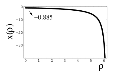
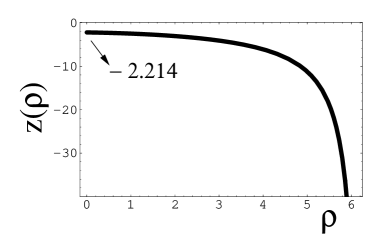
FIG. 5.: In the case $\Lambda=-2$ and $\epsilon=0.1$ the numerical integration of the system (5.2) is reported. The initial conditions are given in a critical point of the system , namely the point $(x_{1},\,z_{1})$ reported in Eq. (4.34).

Again, the proof of this statement can be given by direct numerical integration whose results are reported in Fig. 5.

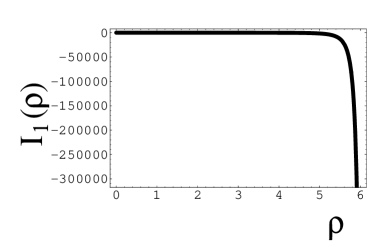
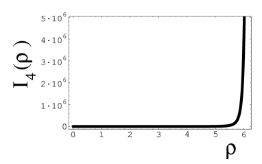
FIG. 6.: The Riemann (left) and Ricci (right) invriants are reported for the numerical solution obtained in Fig. 5.

Numerical examples concerning the case $x\neq y$ will now be given. The specific values of $\epsilon$ and $\Lambda$ are just meant to illustrate some interesting features of the solutions. As a general remark we could say that in the case $x\neq y$ singularities seem to be more likely. This statement is only based on a scan of the numerical solutions for different values of $\Lambda$ and $\epsilon$.

Suppose that $\epsilon=0.1$. Thus, from the examples of Fig. (1), $\Lambda$ needs to be sufficiently negative in order to produce real (negative) roots in Eq. (4.41). Suppose, for instance that $\Lambda=-10$. Then, from Eqs. (4.40)–(4.41), the critical points will be,

$$(x_{1},\,y_{1},\,z_{1})=(-2.0258,\,0.6386,\,-0.1902),\,\,\,$$ (5.22)

$$(x_{2},\,y_{2},\,z_{2})=(-0.6889,\,-3.3432,\,2.0748).$$ (5.23)

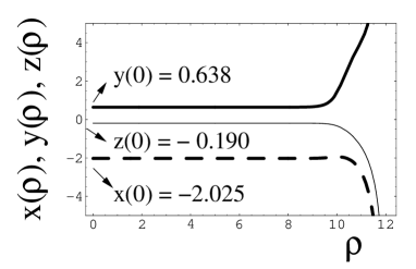
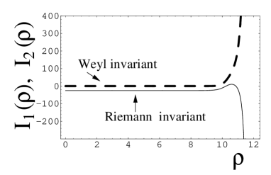
FIG. 7.: In The case of $\Lambda=-10$ and $\epsilon=0.1$ the numerical integration of the system (4.4) is reported in the left plot. The evolution of $x$ (dashed line), $y$ (full thick line) and $z$ (thin line) are illustrated when the initial conditions are given in $(x_{1},y_{1},z_{1})$ of Eq. (4.36). In the plot at the right the Weyl (dashed line) and the Riemann (full line) are reported.

If the initial conditions for the warp factors and for the dilaton are set in $(x_{1},\,y_{1},\,z_{1})$ of Eq. (4.36) then the results of the numerical integration are reported in Fig. 7. A physical singularity is developed at a finite value of $\rho$ where both the Weyl and the Riemann invariant blow up. The same kind of solutions can be obtained if the initial conditions are set not in $(x_{2},\,y_{2},\,z_{2})$ of Eq. (5.23). Also in this second case a singularity is developed at finite $\rho$.

In order to describe the qualitative behavior of the system the value of $\epsilon$ can be changed. From Fig. 1 (left plot) $\Lambda=-2$ can be selected and from Eqs. (4.40)–(4.41) the critical points are found to be

$$(x_{1},\,y_{1},\,z_{1})=(-0.8679,\,0.6052,\,-0.2419),$$ (5.24)

$$(x_{2},\,y_{2},\,z_{2})=(-0.1638,\,-3.5390,\,0.9350).$$ (5.25)

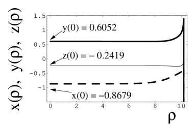
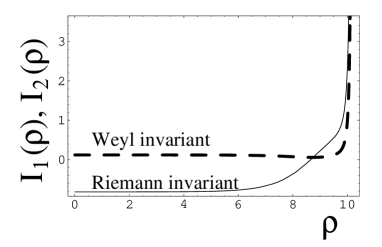
FIG. 8.: In the left plot the numerical integration of eqs. (4.4) is illustrated for $\Lambda=-2$ and $\epsilon=0.1$. The notations are exactly the same as in Fig. 7. The initial conditions are given in the point $(x_{1},y_{1},z_{1})$ reported in Eq. (5.25).

In this case the results of the numerical integration are reported in Fig. 8. Also in this example a physical singularity is developed at finite value of $\rho$.

In the present Section we examined systematically the critical points of the dynamical system arising from the low energy $\beta$ functions truncated to first order in the string tension corrections. For practical purposes two cases have been distinguished namely the one where the warp factors are proportional and the one where the warp factors are both exponentially decreasing but not proportional to each other. From the analysis of both cases we can conclude that there are no (stable) critical points of the $\beta$-functions where the dilaton is frozen. This means that stable (or unstable) critical points with decreasing dilaton field cannot be analytically connected with solutions where the dilaton coupling is frozen to a constant value. However, a large class of critical points leads to warped compactifications in the sense that the warp factors are exponentially decreasing and the dilaton coupling is also exponentially decreasing (without getting fixed to a constant value).

As pointed out in the introduction, the present investigation suffers from various limitations. That is why the present results can only be considered as illustrative. However, it is not unreasonable that some of the nasty features of the present results might be changed if thick branes are included. In this case some of the unstable solutions might get stabilized since a new scale (the thickness of the brane) arises in the problem. For instance solutions with exponentially decreasing warp factors and decreasing dilaton coupling might turn into warped solutions with constant dilaton. On the contrary warped solutions with increasing dilaton coupling (corresponding to another class of fixed points emerging from the present analysis) might be driven towards naked singularities with Kasner-like features.

VI Concluding Remarks

The effects of the dilaton and of higher order curvature terms are usually neglected in the context of six dimensional warped compactification. This is certainly a consistent assumption which can be, however, relaxed. In the present investigation six-dimensional warped compactification has been analyzed in the context of the gravity theory inspired by the low energy string effective action. Tree-level solutions have been derived. First order $\alpha^{\prime}$ corrections have been also included precisely in the form induced by string amplitudes.

The tree-level solutions exhibit a Kasner-like branch whose generic property is the occurrence of curvature singularities. In this case the warp factors are powers of the bulk radius $\rho$. The powers satisfy specific sum rules leading ultimately to divergences in the curvature invariants. The features of the tree-level solutions (as a function of the bulk radius) are the static analog of the time-dependent case which has been widely exploited in cosmological considerations. Kasner-like solutions can be found both for vanishing and non vanishing bulk cosmological constant. This means that, at tree-level, exponentially decreasing warp factors cannot be generically obtained. Moreover, since the Kasner-like behaviour leads to curvature singularities, there will be a regime where the solutions hit the string curvature scale where higher order string tension corrections cannot be neglected.

The inclusion of the first order $\alpha^{\prime}$ correction produces computable modifications in the $\beta$-functions which can be viewed, for the present purpose, as a nonlinear dynamical system. Solutions with exponentially decreasing warp factors become then possible: they correspond to critical points of the dynamical system. Defining ${\cal H}=\partial_{\rho}\ln{\sigma}$ and ${\cal F}=\partial_{\rho}\ln{\gamma}$ interesting critical points can be obtained in the case of constant (and negative) ${\cal H}$ and ${\cal F}$. These critical points correspond to linear (decreasing) dilaton solutions.

The obtained critical points are not always stable. It can happen that a given critical point correspond to stable/unstable node or to stable/unstable spiral points. In the case ${\cal H}={\cal F}$ the Kasner branch of the solution (for $\rho\sim 0$) can be analytically connected to a critical point. There are also solutions where two critical points can be analytically connected. In this case a given ${\cal H}_{1}<0$ turns into ${\cal H}_{2}\neq{\cal H}_{1}$. Unfortunately in the numerical examples analyzed in the present investigation ${\cal H}_{2}>0$.

In the case ${\cal H}\neq{\cal F}$ the situation is mathematically more complicated. By giving initial conditions of the system near a critical point singularities seem to be developed. Numerical evidence of this behavior has been presented by studying the singularity properties of the curvature invariants.

It is now the moment of comparing what we have with what we ought to have. The ideal situation would be to find stable fixed points of the low energy $\beta$ functions compatible with a constant dilaton field. In other words it would be nice to find solutions interpolating between a singularity and a critical point of constant dilaton or between an unstable critical point and a constant dilaton solution. Such a behavior would give rise to exponentially decreasing warp factors with constant dilaton coupling which is exactly the original assumption tacitly adopted in five and six-dimensional warped compactifications. This situation is never realized in the set-up described in the present investigation but it cannot be excluded in principle in slightly different frameworks. It has been shown that exponentially decreasing warp factors are certainly compatible with the low energy string effective action, however, the obtained critical points do not have the wanted physical properties. These results should not be viewed as conclusive and might only be due to the limitations of the present analysis.

We will now speculate about various possibilities which might cure the limitations of our approach allowing, hopefully, for stable critical points with frozen dilaton. As we discussed the first (obvious) limitation which should be relaxed concerns the dilaton dynamics. In the present paper only string tension corrections have been considered. In principle one can expect that corrections in the dilaton coupling should also be included for consistency since they become relevant roughly at the same scale at which string tension corrections are turned on. Following a complementary way of thinking one can also try to account for the effect of the dilaton potential which has been also (partially) neglected since we modeled it with a cosmological constant. An encouraging remark, in this direction, would be that already within our over-simplified set-up decreasing dilaton solutions were compatible with exponentially decreasing warp factors. These solutions might be analytically connected with a critical point of constant dilaton once a dilaton potential is present. A less encouraging evidence is however that constant dilaton solutions are obtained (within the present analysis) only as $1/\alpha^{\prime}$ effect. These solutions are clearly non-perturbative and it might be that only by summing up all the string tension corrections a definite answer can be obtained.

Another limitation of the present analysis is the absence of realistic (thick) brane sources. It is not unreasonable to expect that by adding a brane of finite thickness in the game some of the unstable critical points of the system will be stabilized at a constant value of the dilaton coupling fixed, presumably, by the tension of the brane. This possibility should be further scrutinized. Again an encouraging hint in this direction is that, already at the level of our analysis, it is possible to connect a critical point to Kasner-like solutions.

Furthermore in our analysis we completely neglected the possible presence of $p$-form fields whose effect should also be studied. To neglect the antisymmetric field strength is consistent if we look at the explicit form of the first string tension correction. However, an antisymmetric tensor field with large magnetic component might introduce qualitatively new solutions. In the present discussion the antisymmetric tensor field has been frozen. However, once an antisymmetric tensor is allowed on the same footing of the other light modes the structure of the string tension corrections changes radically: higher powers of the field strength will appear to first order in the string tension corrections. We leave all these themes for forthcoming investigations.

Finally, some cosmological implications of our work should be mentioned. Once thick branes, antisymmetric tensor field and dilaton potetial will be taken into account in simplified models, time dependent solutions might be studied. In this case the problem will certainly be more complicated but not totally hopeless if stable critical points of the truncated $\beta$ functions will be found in the time-independent case. We also leave these topics for future investigations.

A Curvature Invariants

In order to scrutinize the singularity properties of the six-dimensional metric discussed in the present investigation the quadratic curvature invariants should be properly discussed. The curvature invariants computed from Eq. (1.1) can be written as

$$I_{1}(\rho)=R_{\mu\nu\alpha\beta}R^{\mu\nu\alpha\beta}=\frac{1}{4}[{\cal F}^{4}-6{\cal H}^{4}+4{\cal F}^{2}{\cal F}^{\prime}+4{\cal F}^{\prime 2}+16{\cal H}^{2}{\cal H}^{\prime}+16{\cal H}^{\prime 2}]$$ (A.1)

$$I_{2}(\rho)=C_{\mu\nu\alpha\beta}C^{\mu\nu\alpha\beta}=\frac{3}{20}[2({\cal H}^{\prime}-{\cal F}^{\prime})+{\cal F}({\cal H}-{\cal F})]^{2}$$ (A.2)

$$I_{3}(\rho)=R=\frac{1}{2}[\frac{3}{2}{\cal F}^{2}+4{\cal H}{\cal F}+10{\cal H}^{2}+2{\cal F}^{\prime}+8{\cal H}^{\prime}]$$ (A.3)

$$I_{4}(\rho)=R_{\mu\nu}R^{\mu\nu}=\frac{1}{8}[{\cal F}^{4}+4{\cal H}{\cal F}^{3}+14{\cal H}^{2}{\cal F}^{2}+16{\cal H}^{3}{\cal F}+40{\cal H}^{4}+4{\cal F}^{2}{\cal F}^{\prime}$$ (A.4)

$$+8{\cal H}{\cal F}{\cal F}^{\prime}+8{\cal H}^{2}{\cal F}^{\prime}+4{\cal F}^{\prime 2}+8{\cal F}^{2}{\cal H}^{\prime}+8{\cal H}{\cal F}{\cal H}^{\prime}+64{\cal H}^{2}{\cal H}^{\prime}+16{\cal H}^{\prime}{\cal F}^{\prime}+40{\cal H}^{\prime 2}]$$ (A.5)

The Weyl invariant vanishes in the case where $\sigma(\rho)$ and $\gamma(\rho)$ are proportional, namely in the case where ${\cal H}\equiv{\cal F}$. The other invariants are do not vanish in the limit ${\cal H}\rightarrow{\cal F}$ .

The curvature invariant are singular in the case of the tree-level solutions derived in Eqs. (2.9). For instance the Riemann and Weyl invariants can be written, for the solutions of Eqs. (2.9), as:

$$I_{1}(\rho)=\frac{\Lambda^{2}}{16}\,[4\,\alpha^{2}-12\,\alpha^{4}+\beta^{2}+2\,\beta^{4}-4\,\left(4\,\alpha^{3}+\beta^{3}\right)\,\cosh{[{\sqrt{-\Lambda}}\,(\rho-\rho_{0})]}$$ (A.6)

$$+\left(4\,\alpha^{2}+\beta^{2}\right)\,\cosh{[2\,{\sqrt{-\Lambda}}\,(\rho-\rho_{0})]}]\,{\sinh{[{\sqrt{-L}}\,(\rho-\rho_{0})]}}^{-4},$$ (A.7)

$$I_{2}(\rho)=\frac{3}{40}\left(\alpha-\beta\right)^{2}\,\Lambda^{2}\,{\left(\beta-\cosh{[{\sqrt{-\Lambda}}\,(\rho-r_{0})]}\right)}^{2}\,{\sinh{[{\sqrt{-\Lambda}}\,(\rho-\rho_{0})]}}^{-4}.\,$$ (A.8)

This shows that the tree-level (Kasner-like) solutions are indeed singular for $\rho\rightarrow\rho_{0}$. Notice, again, that if $\alpha=\beta$ the solution still exists. In this case the Weyl invariant vanishes identically but the Riemann invariant (and the other invariants) are still singular.

In order to detect singularities in a given solution the behavior of the curvature invariants has been scrutinized as a function of the bulk radius. This is a consistent procedure. In order to fully analyze the singularity properties of the solution we should also investigate the behavior of non-space-like geodesics (i.e. either time-like or null). This check is pleonastic if the curvature invariants diverge. However, the regularity of the curvature invariants is a necessary but not sufficient condition in order to assess the regularity of a manifold. In principle, in order to claim that a given geometry is singularity-free we should chack that the curvature invariants are regular and that non-space-like geodesics are complete (i.e. they can be extended to any value of the affine parameter). These are the usual general relativity criteria for the analysis of physical singularities of a given space-time. Using Einstein equations together with topological considerations these criteria can be rephrased in terms of energy conditions involving the various components of the energy momentum tensor. Hawking-Penrose theorems are based on this type of considerations [31].

When singularities are analyzed in the context of the low-energy string effective action there is a further ambiguity related to the choice of the physical frame where the calculation is performed. In this paper the string frame parameterization of the action has been used. Other frames can be anyway defined. A very useful frame is the Einstein frame where the dilaton and the graviton are decoupled (at tree-level). Defining as $g_{\mu\nu}$ a $D=4+n$ dimensional metric in the string frame and as $G_{\mu\nu}$ as the Einstein frame metric (in the same number of dimensions) we have that they are related through a conformal rescaling involving the string frame dilaton $\phi$, namely:

$$G_{\mu\nu}=e^{-\frac{2\phi}{n+2}}g_{\mu\nu}.$$ (A.9)

The (canonically normalized) Einstein frame dilaton ($\varphi$) is simply related to $\phi$ as $\varphi=\phi\sqrt{2/(n+2)}$. The transformation of Eq. (A.9) clearly induces a change in the curvature invariants. Consider, for instance, the scalar curvature in the string frame and call it $R$. In the Einstein frame the scalar curvature will be ${\cal R}$. The relation between $R$ and ${\cal R}$ is

$$R=e^{-\psi}\biggl{[}{\cal R}-(n+3)G^{\alpha\beta}\nabla_{\alpha}\nabla_{\beta}\psi-\frac{(n+3)(n+2)}{4}G^{\alpha\beta}\nabla_{\alpha}\psi\nabla_{\beta}\psi\biggr{]},$$ (A.10)

where $\psi=\varphi\sqrt{2/(n+2)}$ and where the covariant derivatives are computed with respect to $G_{\mu\nu}$. The two frames certainly describe the same physics even if there has been debate on which of the two frames captures better the stringy features of a given solution of the low-energy $\beta$-functions. As far as the singularity properties are concerned we can clearly see that the two frames are not equivalent. Suppose, for instance, that the dilaton field is decreasing in the Einstein frame and suppose that ${\cal R}$ is regular in the same frame. Then Eq. (A.10) tells that $R$ will be no longer regular in the string frame. Therefore singularities may appear and disappear from one frame to the other.

This example only means that the two frames are indeed physically equivalent when we deal with physical solutions namely solutions where the dilaton is asymptotically constant, for instance. This observation helps in setting the goals of the present paper. We want warped compactifications, corresponding to stable critical points of the truncated $\beta$-functions for which the dilaton field is frozen to a constant value.

A similar situation [32] occurs in another type of inhomogeneous backgrounds (i.e. four-dimensional background geometries with two commuting Killing vectors which are hypersurface orthogonal and orthogonal to each others). In [32] completely regular and geodesically complete solutions of the low-energy $\beta$ functions have been discussed in the framework of these backgrounds. Also in the case [32] the crucial requirement is that the dilaton interpolates between two constant values.

B Equations of motion with the first $\alpha^{\prime}$ correction

Inserting the metric given in Eq. (1.1) into Eq. (3.6) the reduced form of the action is obtained to first order in $\alpha^{\prime}$, namely

$$S=-\frac{1}{2\lambda_{s}^{4}}\int d^{4}x\,\int d\rho\,\,d\theta\,\,\,\,\sigma^{2}\,\,\sqrt{\gamma}\,\,e^{-\phi}\,\,\{\frac{{\cal F}^{2}}{2}+5{\cal H}^{2}+2{\cal H}{\cal F}+4\partial_{\rho}{\cal H}+\partial_{\rho}{\cal F}-(\partial_{\rho}\phi)^{2}+\Lambda$$ (B.1)

$$-\epsilon[3{\cal H}^{2}{\cal F}^{2}+\frac{15}{2}{\cal H}^{4}+6{\cal H}^{2}\partial_{\rho}{\cal F}+12{\cal H}{\cal F}\partial_{\rho}{\cal H}+12{\cal H}^{3}{\cal F}+12{\cal H}^{2}\partial_{\rho}{\cal H}-(\partial_{\rho}\phi)^{4}]\}.$$ (B.2)

Recalling now that ${\cal H}=\partial_{\rho}\ln{\sigma}$ and that ${\cal F}=\partial_{\rho}\ln{\gamma}$ we can perform, separately, the variation with respect to $\phi$, $\sigma$ and $\gamma$. The variation with respect to $\phi$ gives

$$-2\,{\Lambda}-{{\cal F}}^{2}-4\,{\cal F}\,{\cal H}-10\,{{\cal H}}^{2}-2\,{\cal F}^{\prime}-8\,{\cal H}^{\prime}+2\,{\cal F}\,{\phi}^{\prime}+8\,{\cal H}\,{\phi}^{\prime}-2\,{{\phi}^{\prime}}^{2}+4\,{\phi}^{\prime\prime}$$ (B.3)

$$+\epsilon\,(6\,{{\cal F}}^{2}\,{{\cal H}}^{2}+24\,{\cal F}\,{{\cal H}}^{3}+15\,{{\cal H}}^{4}+12\,{{\cal H}}^{2}\,{\cal F}^{\prime}+24\,{\cal F}\,{\cal H}\,{\cal H}^{\prime}+24\,{{\cal H}}^{2}\,{\cal H}^{\prime}$$ (B.4)

$$-4\,{\cal F}\,{{\phi}^{\prime}}^{3}-16\,{\cal H}\,{{\phi}^{\prime}}^{3}+6\,{{\phi}^{\prime}}^{4}-24\,{{\phi}^{\prime}}^{2}\,{\phi}^{\prime\prime})=0,$$ (B.5)

whereas the variation with respect to $\sigma$ and $\gamma$ gives

$$f_{3}^{\prime\prime}(\rho)+2({\cal H}+\frac{{\cal F}}{2}-\phi^{\prime})f_{3}^{\prime}(\rho)-f_{2}^{\prime}(\rho)-({\cal H}+\frac{{\cal F}}{2}-\phi^{\prime})f_{2}(\rho)$$ (B.6)

$$+\biggl{[}({\cal H}+\frac{{\cal F}}{2}-\phi^{\prime})^{2}+({\cal H}^{\prime}+\frac{{\cal F}^{\prime}}{2}-\phi^{\prime\prime})\biggr{]}f_{3}(\rho)+f_{1}(\rho)=0,$$ (B.7)

$$g_{3}^{\prime\prime}(\rho)+2(2{\cal H}-\frac{{\cal F}}{2}-\phi^{\prime})g_{3}^{\prime}(\rho)-g_{2}^{\prime}(\rho)-(2{\cal H}-\frac{{\cal F}}{2}-\phi^{\prime})g_{2}(\rho)$$ (B.8)

$$+\biggl{[}(2{\cal H}-\frac{{\cal F}}{2}-\phi^{\prime})^{2}+(2{\cal H}^{\prime}-\frac{{\cal F}^{\prime}}{2}-\phi^{\prime\prime})\biggr{]}g_{3}(\rho)+g_{1}(\rho)=0$$ (B.9)

where the $f(\rho)$ are given by

$$f_{1}(\rho)=2\,\Lambda-2\,{\cal F}\,{\cal H}+{\left({\cal F}+2\,{\cal H}\right)}^{2}+2\,\left({\cal F}^{\prime}+2\,{\cal H}^{\prime}\right)-2\,{{\phi}^{\prime}}^{2}+\epsilon\,\left(3\,{{\cal H}}^{4}+12\,{{\cal H}}^{2}\,{\cal H}^{\prime}+2\,{{\phi}^{\prime}}^{4}\right),$$ (B.10)

$$f_{2}(\rho)=2\,\left({\cal F}+{\cal H}\right)-6\,\epsilon\,\left[{{\cal H}}^{3}+{\cal F}\,{\cal H}\,\left(2\,{\cal H}+{\cal F}\right)+4\,{\cal H}\,{\cal H}^{\prime}+2\,\left({\cal H}\,{\cal F}^{\prime}+{\cal F}\,{\cal H}^{\prime}\right)\right],$$ (B.11)

$$f_{3}(\rho)=4[1-3\,\epsilon\,{\cal H}\,\left({\cal F}+{\cal H}\right)],$$ (B.12)

and the $g(\rho)$ are given by

$$g_{1}(\rho)=\frac{1}{4}\biggl{[}2\,{\Lambda}+{{\cal F}}^{2}-4\,{\cal F}\,{\cal H}+10\,{{\cal H}}^{2}-2\,{\cal F}^{\prime}+8\,{\cal H}^{\prime}-2\,{{\phi}^{\prime}}^{2},$$ (B.13)

$$-\epsilon\,\left(6\,{{\cal F}}^{2}\,{{\cal H}}^{2}-24\,{\cal F}\,{{\cal H}}^{3}+15\,{{\cal H}}^{4}-12\,{{\cal H}}^{2}\,{\cal F}^{\prime}-24\,{\cal F}\,{\cal H}\,{\cal H}^{\prime}+24\,{{\cal H}}^{2}\,{\cal H}^{\prime}-2\,{{\phi}^{\prime}}^{4}\right)\biggr{]},$$ (B.14)

$$g_{2}(\rho)=-{\cal F}+2\,{\cal H}-6\,\epsilon\,\left(-{\cal F}\,{{\cal H}}^{2}+2\,{{\cal H}}^{3}+2\,{\cal H}\,{\cal H}^{\prime}\right),$$ (B.15)

$$g_{3}(\rho)=1-6\,\epsilon\,{{\cal H}}^{2}.$$ (B.16)

Recall that ${}^{\prime}=\partial_{\rho}$. Eq. (B.5) exactly coincides with Eq. (3.18). Inserting Eqs. (B.12)–(B.16) into Eqs. (B.7) and (B.5) we get, respectively, Eqs. (3.12) and (3.15).

C Eigenvalues around the critical points

The two eigenvalues in the case of $\Lambda<0$ can be written as

$$W_{1}(k)=\sqrt{\frac{5\,\Lambda_{-}}{2}}{\sqrt{1+{\sqrt{1+\frac{212\,k}{5}}}}}\frac{\biggl{(}T(k)+\sqrt{S(k)Q(k)}\biggr{)}}{V(k)}$$ (C.1)

$$W_{2}(k)=\sqrt{\frac{5\,\Lambda_{-}}{2}}{\sqrt{1+{\sqrt{1+\frac{212\,k}{5}}}}}\frac{\biggl{(}T(k)-\sqrt{S(k)Q(k)}\biggr{)}}{V(k)}$$ (C.2)

where

$$T(k)=\frac{1}{2}\biggl{\{}-1925-260180\,k-7570944\,k^{2}+5\,{\sqrt{1+\frac{212\,k}{5}}}\,[385+384\,k\,\left(-19+792\,k\right)]\biggr{\}}$$ (C.3)

$$S(k)=\biggl{\{}1015+99916\,k+2411712\,k^{2}-{\sqrt{1+\frac{212\,k}{5}}}\,[1015+12\,k\,\left(2269+158400\,k\right)]\biggr{\}}$$ (C.4)

$$Q(k)=\biggl{\{}125+123380\,k+5006592\,k^{2}+5\,{\sqrt{1+\frac{212\,k}{5}}}\,[-25+48\,k\,\left(563+12672\,k\right)]\biggr{\}}$$ (C.5)

$$V(k)=\,k\,[127925+576\,k\,\left(12473+348480\,k\right)]$$ (C.6)

Recall that $k=\epsilon\Lambda_{-}$.

REFERENCES

• [1] V. Rubakov and M. Shaposhnikov, Phys. Lett. B 125, 136 (1983).
• [2] V. Rubakov and M. Shaposhnikov, Phys. Lett. B 125, 139 (1983).
• [3] K.Β Akama, in Proceedings of the Symposium on Gauge Theory and Gravitation, Nara, Japan, eds. K.Β Kikkawa, N.Β Nakanishi and H.Β Nariai (Springer-Verlag, 1983),[hep-th/0001113].
• [4] M.Β Visser, Phys.Β Lett.Β  B159 (1985) 22 [hep-th/9910093].
• [5] S. Randjbar-Daemi and C. Wetterich, Phys. Lett. B 166, 65 (1986).
• [6] A. G. Cohen and D. B. Kaplan, Phys. Lett. B 470, 52 (1999).
• [7] A. Chodos and E. Poppitz, Phys. Lett. B 471, 119 (1999); A. Chodos, E. Poppitz and D. Tsimpis [hep-th/0006093].
• [8] I. Olasagasti and A. Vilenkin, Phys. Rev. D 62, 044014 (2000).
• [9] R. Gregory, Phys. Rev. Lett. 84, 2564 (2000).
• [10] T. Gherghetta and M. Shaposhnikov, Phys.Rev.Lett. 85, 240 (2000).
• [11] I. Oda [hep-th/0006203]; S. Hayakawa and K. I. Izawa, [hep-th/0008111].
• [12] J. Chen, M. Luty, and E. Ponton, JHEP 0009, 012 (2000).
• [13] L. Randall and R. Sundrum, Phys.Rev. Lett. 83, 3370 (1999).
• [14] J. E. Kim, B Kyae and H. M. Lee, [hep-th/0004005]; I. Low and A. Zee, [hep-th/0004124].
• [15] S. Nojiri and S. D. Odintsov JHEP 0007, 49 (2000); S. Nojiri, S. D. Odintsov, and S. Ogushi, [hep-th/0010004]; K. A. Meissner and M. Olechowski, [hep-th/0009122].
• [16] I. Neupane, [hep-th/0008191].
• [17] N. Mavromatos and J. Rizos, [hep-th/0008074].
• [18] M. Giovannini, UNIL-IPT-00-20 [hep-th/0009172].
• [19] C. Lovelace, Phys. Lett. B 135, 75 (1984); E. S. Fradkin abd A. A. Tseytlin, Nucl. Phys. B 261, 1 (1985).
• [20] C. G. Callan, D. Friedan, E. J. Martinec and, M. J. Perry Nucl. Phys. B 262; A. Sen, Phys. Rev. Lett. 55, 1846 (1985).
• [21] R. R. Metsaev and A. A. Tseytlin, Phys. Lett. B 191, 115 (1987); Nucl. Phys. B 293, 385 (1987).
• [22] B. Zwiebach, Phys. Lett. B 156, 315 (1985).
• [23] D. G. Boulware and S. Deser, Phys. Rev. Lett. 55, 2656 (1985); Phys. Lett. B 175, 409 (1986).
• [24] N. E. Mavromatos and J. L. Miramontes, Phys. Lett. B 201, 473 (1988).
• [25] G. Veneziano, Phys. Lett. B 265, 287 (1991); String Cosmology: the Pre-Big-Bang Scenario CERN-TH-2000-042 Lectures given at 71st Les Houches Summer School β€œThe Primordial Universe” , Les Houches (France) 28 Jun - 23 Jul 1999, [ hep-th/0002094].
• [26] J. Madore, Phys. Lett. A 110, 289 (1985); Phys. Lett. A 111, 283 (1985).
• [27] M. Gasperini and M. Giovannini, Phys. Lett. B 287, 56 (1991).
• [28] I. Antoniadis, J. Rizos, and K. Tamvakis Nucl.Phys.B 415, 497 (1994); J. Rizos and K. Tamvakis, Phys.Lett. B326, 57 (1994).
• [29] J. Maldacena and C. Nunez, [hep-th/0007018].
• [30] R. Grimshaw, Nonlinear Ordinary Differential Equations, (Blackwell Scientific Publications, 1990).
• [31] S. W. Hawking and G. F. R. Ellis, The large Scale Structure of the Universe (Cambridge University Press, Cambridge, England, 1973).
• [32] M. Giovannini, Phys. Rev. D 59, 083511 (1999); Phys. Rev. D 57, 7223 (1998).