Tachyon Condensation
in
Cubic Superstring Field Theory

Abstract

It has been conjectured that at the stationary point of the tachyon potential for the non-BPS $\mathrm{D}$-brane or brane-anti-$\mathrm{D}$-brane pair, the negative energy density cancels the brane tension. We study this conjecture using a cubic superstring field theory with insertion of a double-step inverse picture changing operator. We compute the tachyon potential at levels $(1/2,\,1)$ and $(2,\,6)$. In the first case we obtain that the value of the potential at the minimum is $97.5\%$ of the non BPS D-brane tension. Using a special gauge in the second case we get $105.8\%$ of the tension.

1 Introduction

One of the main motivation to construct string field theory (SFT) [1, 2] was a hope to study non-perturbative phenomena in string theory. SFT gives an off-shell formulation of a string theory providing a possibility to investigate non-perturbative phenomena in a systematic way.

The bosonic open string has a tachyon that leads to an instability of a perturbative vacuum. In the early works by Kostelecky and Samuel [3] it was proposed to use SFT to describe condensation of the tachyon to a stable vacuum. They have shown that a truncation of open SFT at low levels gives a rather systematic approximation scheme to calculate the tachyon effective potential. Moreover, within this calculation scheme the tachyon potential in open bosonic string has a nontrivial minimum.

Further [4], the level truncation method has been applied to examine an effective potential of auxiliary fields in a cubic superstring field theory (SSFT) [5, 6, 7]. It was found that some of the low-lying auxiliary scalar fields acquire non-zero vacuum expectation values providing a new mechanism for supersymmetry breaking. The gauge vector field becomes massive while the physical spinor remains massless, thus the supersymmetry is broken in the nonperturbative vacuum.

Recently, Sen has proposed [8] to interpret the tachyon condensation as a decay of an unstable D-brane. In the framework of this interpretation the vacuum energy of the open bosonic string in the Kostelecky and Samuel vacuum has to cancel the tension of the unstable D-brane (more precisely a difference between Kostelecky and Samuel vacuum and the unstable perturbative vacuum should be equal to the tension of the unstable D-brane). In the cubic SFT this cancellation has been checked [9] at the low levels. Further it was argued that the value of the tachyon potential at the minimum cancels $99\%$ of bosonic D-brane’s tension [10].

The tachyon potential has been also evaluated in non-polynomial [11] open NS string field theory [12]. Note that the tachyon comes from GSO$-$ sector and calculations involve only the NS string. Later on [13], the calculations have been expanded up to the level $3/2$ and $85\%$ of the non-BPS D-brane’s tension has been cancelled. In the subsequent papers [14] the calculations involving higher levels were performed and the value of the tachyon potential at the minimum was found to cancel $90.5\%$ of the brane tension.

In this note we compute the tachyon potential at low levels of cubic SSFT. We also find nontrivial minimum with the value of potential being $105.8\%$ of the brane tension.

The paper is organized as follows. Section 2 contains a brief review of cubic SSFT. In Section 3 the actual calculations of the tachyon potential up to the second nontrivial level are performed. In Section 4 we determine the brane tension in cubic theory. Appendices contain necessary information and proof of the odd bracket properties .

2 Superstring Field Theory on the Branes

2.1 Cubic Super String Field Theory

The original Witten’s proposal [2] for NSR superstring field theory action reads (we list only NS sector, relevant for the following):

$$S_{W}\cong\int\mathcal{A}\star Q_{B}\mathcal{A}+\frac{2}{3}\int\mathrm{X}\mathcal{A}\star\mathcal{A}\star\mathcal{A}.$$ (2.1)

Here $Q_{B}$ is the BRST charge, $\int$ and $\star$ are Witten’s string integral and star product to be specified below. The string field $\mathcal{A}$ is a series with each term being a state in the Fock space $\mathcal{H}$ multiplied by space-time field. States in $\mathcal{H}$ are created by the modes of the matter fields $X^{\mu}$ and $\psi^{\mu}$, conformal ghosts $b,\,c$ and superghosts $\beta,\,\gamma$:

$$\mathcal{A}=\sum A_{i\dots}(x)\,\beta_{i}...\gamma_{j}...b_{k}...c_{l}...\alpha^{\mu}_{n}...\psi^{\nu}_{m}|0\rangle_{-1}.$$ (2.2)

The characteristic feature of the action (2.1) is the choice of the $-1$ picture for the string field $\mathcal{A}$. The vacuum $|0\rangle_{-1}$ in the NS sector is defined as

$$|0\rangle_{-1}=c(0)e^{-\phi(0)}|0\rangle,$$ (2.3)

where $|0\rangle$ stands for $SL(2,\mathbb{R})$-invariant vacuum and $\phi$ is the field ”bosonizing” the $\beta,\,\gamma$ system: $\gamma=\eta e^{\phi}$, $\beta=e^{-\phi}\partial\xi$. The insertion of the picture-changing operator [15]

$$\mathrm{X}=\frac{1}{\alpha^{\,\prime}}e^{\phi}\psi\cdot\partial X+c\partial\xi+\frac{1}{4}b\partial\eta e^{2\phi}+\frac{1}{4}\partial(b\eta e^{2\phi})$$ (2.4)

in the cubic term is just aimed to absorb the unwanted unit of the $\phi$ charge as only $\langle 0|e^{-2\phi}|0\rangle\neq 0$.

The action (2.1) suffers from the contact term divergencies [16, 17, 18, 19] which arise when a pair of $\mathrm{X}$-s collides in a point. This sort of singularities appears already at the tree level. To overcome this trouble it was proposed to change the picture of NS string fields from $-1$ to $0$, i.e. to replace $|0\rangle_{-1}$ in (2.2) by $|0\rangle$ [5, 6]. States in the $-1$ picture can be obtained from the states in the $0$ picture by the action of the inverse picture-changing operator $Y$ [15]

$$Y=4c\partial\xi e^{-2\phi}$$

with $\mathrm{X}Y=Y\mathrm{X}=1$. This identity holds outside the ranges $\ker\mathrm{X}$ and $\ker Y$. Therefore at the $0$ picture there are states that can not be obtained by applying the picture changing operators $\mathrm{X}$ and $Y$ to the states at the $-1$ picture.

The action for the NS string field in the $0$ picture has the cubic form with the insertion of a double-step inverse picture-changing operator $Y_{-2}$ [5, 6]:

$$S\cong\int Y_{-2}\mathcal{A}\star Q_{B}\mathcal{A}+\frac{2}{3}\int Y_{-2}\mathcal{A}\star\mathcal{A}\star\mathcal{A}.$$ (2.5)

We discuss $Y_{-2}$ in the next subsection.

In the description of the open NSR superstring the string field $\mathcal{A}$ is subjected to be GSO$+$. In the $0$ picture there is a variety of auxiliary fields as compared with the $-1$ picture. These fields are zero by means of the free equation of motion: $Q_{B}\mathcal{A}=0$, but they play a significant role in the off-shell calculations. For instance, a low level off-shell NS string field expands as

$$\mathcal{A}\cong\int dk\;\{ u(k)c_{1}-\frac{1}{2}A_{\mu}(k)ic_{1}\alpha_{-1}^{\mu}-\frac{1}{4}B_{\mu}(k)\gamma_{\frac{1}{2}}\psi_{-\frac{1}{2}}^{\mu}$$

$$+\frac{1}{2}F_{\mu\nu}(k)c_{1}\psi_{-\frac{1}{2}}^{\mu}\psi_{-\frac{1}{2}}^{\nu}+B(k)c_{0}+r(k)c_{1}\gamma_{\frac{1}{2}}\beta_{-\frac{3}{2}}+\dots\}e^{ik\cdot X(0,0)}|0\rangle.$$

Here $u$ and $r$ are just the auxiliary fields mentioned above.

The SSFT based on the action (2.5) is free from the drawbacks of the Witten’s action (2.1). The absence of contact singularities can be explained shortly. Really, the tree level graphs are generated by solving the classical equation of motion by perturbation theory. For Witten’s action (2.1) the equation reads

$$Q_{B}\mathcal{A}+\mathrm{X}\mathcal{A}\star\mathcal{A}=0.$$

The first nontrivial iteration ($4$-point function) involving the pair of $\mathrm{X}A\star A$ vertices produces the contact term singularity when two of $\mathrm{X}$-s collide in a point. In contrast, the action (2.5) yields the following equation

$$Y_{-2}(Q_{B}\mathcal{A}+\mathcal{A}\star\mathcal{A})=0.$$

Outside the $\ker Y_{-2}$ the operator $Y_{-2}$ can be dropped out and therefore the interaction vertex does not contain any insertion leading to singularity. The complete proofs of this fact can be found in [5, 6, 7].

2.2 Double Step Inverse Picture Changing Operator

To have well defined SSFT (2.5) the double step inverse picture changing operator must be restricted to be

a) in accord with the identity:

$$Y_{-2}\mathrm{X}=\mathrm{X}Y_{-2}=Y,$$ (2.6)

b) BRST invariant: $[Q_{B},Y_{-2}]=0,$

c) scale invariant conformal field, i.e. conformal weight of $Y_{-2}$ is $0$,

d) Lorentz invariant conformal field, i.e. $Y_{-2}$ does not depend on momentum.

The point a) provides the formal equivalence between the improved (2.5) and the original Witten (2.1) actions. The points b) and d) are obvious. The point c) is necessary to make the insertion of $Y_{-2}$ compatible with the $\star$-product.

As it was shown in paper [6], there are two (up to BRST equivalence) possible choices for the operator $Y_{-2}$.

The first operator, the chiral one [5], is built from holomorphic fields in the upper half plane and is given by

$$Y_{-2}(z)=-4e^{-2\phi(z)}-\frac{16}{5\alpha^{\,\prime}}e^{-3\phi}c\partial\xi\psi\cdot\partial X(z).$$ (2.7)

The identity (2.6) for this operator reads

$$Y_{-2}(z)\mathrm{X}(z)=\mathrm{X}(z)Y_{-2}(z)=Y(z).$$

This $Y_{-2}$ is uniquely defined by the constraints a) – d).

The second operator, the nonchiral one [6], is built from both holomorphic and antiholomorphic fields in the upper half plane and is of the form:

$$Y_{-2}(z,\overline{z})=Y(z)\widetilde{Y}(\overline{z}).$$ (2.8)

Here by $\widetilde{Y}(\overline{z})$ we denote the antiholomorphic field $4\tilde{c}(\overline{z})\overline{\partial}\tilde{\xi}(\overline{z})e^{-2\tilde{\phi}(\overline{z})}$, where $\tilde{c}(\overline{z}),\,\tilde{\xi}(\overline{z})$ and $\tilde{\phi}(\overline{z})$ are antiholomorphic ghosts of the NSR superstring. For this choice of $Y_{-2}$ the identity (2.6) takes the form:

$$Y_{-2}(z,\overline{z})\mathrm{X}(z)=\mathrm{X}(z)Y_{-2}(z,\overline{z})=\widetilde{Y}(\overline{z}).$$

The issue of equivalence between the theories based on chiral or nonchiral insertions still remains open. The first touch to the problem was performed in [20]. It was shown that the actions for low-level space-time fields are different depending on insertion being chosen.

In the present paper the actual calculations started in Section 3 are based on nonchiral operator $Y_{-2}(z,\overline{z})$, but up to the end of current section general points of the discussion are insensitive to the concrete choice of $Y_{-2}$.

2.3 SSFT in the Conformal Language

For SSFT calculations it is convenient to employ the tools of CFT [21]. States in $\mathcal{H}$ are created by action of vertex operators (taken in the origin) on the conformal vacuum $|0\rangle$. In the conformal language $\int$ and $\star$-product mentioned above are replaced by the odd bracket $\langle\!\langle...|\dots\rangle\!\rangle$, defined as follows

$$\begin{split}\langle\!\langle Y_{-2}|A_{1},\dots,A_{n}\rangle\!\rangle&=\left\langle\,P_{n}\circ Y_{-2}(0,0)\,F_{1}^{(n)}\circ A_{1}(0)\dots F_{n}^{(n)}\circ A_{n}(0)\right\rangle\\ &=\left\langle\,F_{j}^{(n)}\circ Y_{-2}(i,\overline{i})\,F_{1}^{(n)}\circ A_{1}(0)\dots F_{n}^{(n)}\circ A_{n}(0)\right\rangle,\quad n=2,3.\end{split}$$ (2.9)

Here r.h.s. contains $SL(2,\mathbb{R})$ -invariant correlation function of CFT. $A_{j}$ $(j=1,\dots,n)$ are vertex operators and $\{F^{(n)}_{j}\}$ is a set of maps from the upper half unit disc to the upper half plane (see Fig.1)

$$\begin{split}F^{(n)}_{j}=P_{n}\circ f^{(n)}_{j},\quad f^{(n)}_{j}(w)=e^{\frac{2\pi i}{n}(2-j)}\left(\frac{1+iw}{1-iw}\right)^{2/n},\quad j=1,\dots,n,\quad n=2,3;\\ P_{2}(z)=i\frac{1-z}{1+z},\quad P_{3}(z)=\frac{i}{\sqrt{3}}\frac{1-z}{1+z}.\end{split}$$ (2.10)

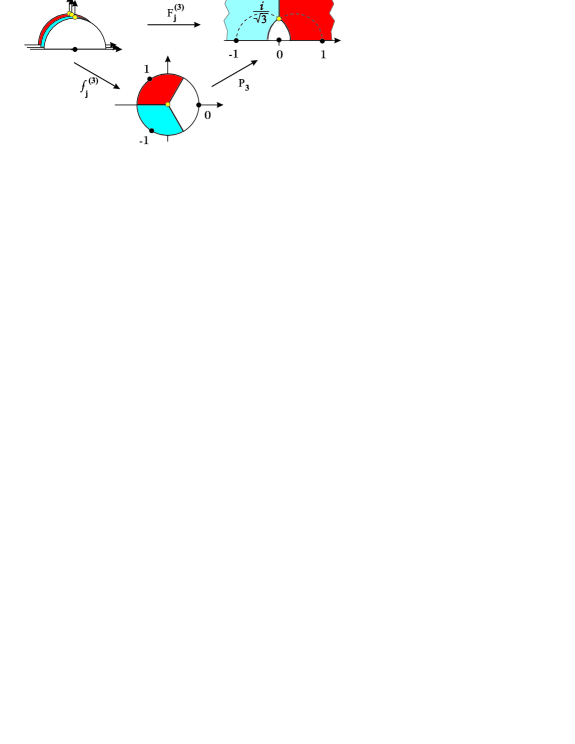
Figure 1: The maps for Witten’s vertex.

By $F\circ A(0)$ we denote the conformal transform of $A$ by $F$. For instance, for a primary field $\mathcal{O}_{h}(z)$ of weight $h$, one gets $F\circ\mathcal{O}_{h}(0)=[F^{\,\prime}(0)]^{h}\mathcal{O}_{h}(F(0))$.

$Y_{-2}$ is the double-step inverse picture changing operator (2.8) inserted in the center of the unit disc. This choice of the insertion point is very important, since all the functions $f_{j}^{(n)}$ maps the points $i$ (the middle points of the individual strings) to the same point that is the origin. In other words, the origin is a unique common point for all strings (see Figure 1). The next important fact is the zero weight of the operator $Y_{-2}$, so its conformal transformation is very simple $f\circ Y_{-2}(z,\overline{z})=Y_{-2}(f(z),\overline{f}(\overline{z}))$. Due to this property it can be inserted in any string. This note shows that the definition (2.9) is self-consistent and does not depend on a choice of a string on which we insert $Y_{-2}$.

Due to the Neumann boundary conditions, there is a relation between holomorphic and antiholomorphic fields. So it is convenient to employ a doubling trick (see details in [22]). Therefore, $Y_{-2}(z,\overline{z})$ can be rewritten in the following form

$$Y_{-2}(z,\overline{z})=Y(z)Y(z^{*}).$$

Here $Y(z)$ is the holomorphic field and $z^{*}$ denotes the conjugated point of $z$ with respect to a boundary, i.e. for the unit disc $z^{*}=1/\overline{z}$ and $z^{*}=\overline{z}$ for the upper half plane. From now on we work only on the whole complex plane. Hence the odd bracket takes the form

$$\langle\!\langle Y_{-2}|A_{1},\dots,A_{n}\rangle\!\rangle=\left\langle\,Y(P_{n}(0))Y(P_{n}(\infty))\,F_{1}^{(n)}\circ A_{1}(0)\dots F_{n}^{(n)}\circ A_{n}(0)\right\rangle.$$ (2.11)

To summarize, the action we start with reads

$$S[\mathcal{A}]=-\frac{1}{g_{o}^{2}}\left[\frac{1}{2}\langle\!\langle Y_{-2}|\mathcal{A},Q_{B}\mathcal{A}\rangle\!\rangle+\frac{1}{3}\langle\!\langle Y_{-2}|\mathcal{A},\mathcal{A},\mathcal{A}\rangle\!\rangle\right],$$ (2.12)

where $g_{o}$ is a dimensionless coupling constant. In Section 4 it will be related to a tension of a $\mathrm{D}$-brane.

2.4 Superstring Field Theory on non-BPS $\mathrm{D}$-brane

To describe the open string states living on a single non-BPS $\mathrm{D}$-brane one has to add GSO$-$ states [23]. GSO$-$ states are Grassman even, while GSO$+$ states are Grassman odd (see Table 1).

Name	Parity	GSO	Comment
$\mathcal{A}_{+}$	odd	$+$	string field in GSO$+$ sector
$\mathcal{A}_{-}$	even	$-$	string field in GSO$-$ sector
$\Lambda_{+}$	even	$+$	gauge
$\Lambda_{-}$	odd	$-$	parameters

Table 1: Parity of string fields and gauge parameters in the 0 picture.

The unique (up to rescaling of the fields) gauge invariant action unifying GSO$+$ and GSO$-$ sectors is found to be

$$\begin{split}S[\mathcal{A}_{+},\mathcal{A}_{-}]&=-\frac{1}{g^{2}_{o}}\left[\frac{1}{2}\langle\!\langle Y_{-2}|\mathcal{A}_{+},Q_{B}\mathcal{A}_{+}\rangle\!\rangle+\frac{1}{3}\langle\!\langle Y_{-2}|\mathcal{A}_{+},\mathcal{A}_{+},\mathcal{A}_{+}\rangle\!\rangle\right.\\ &~{}~{}~{}~{}~{}~{}~{}~{}~{}\left.+\frac{1}{2}\langle\!\langle Y_{-2}|\mathcal{A}_{-},Q_{B}\mathcal{A}_{-}\rangle\!\rangle-\langle\!\langle Y_{-2}|\mathcal{A}_{+},\mathcal{A}_{-},\mathcal{A}_{-}\rangle\!\rangle\right].\end{split}$$ (2.13)

Here the factors before the odd brackets are fixed by the constraint of gauge invariance, that is specified below, and reality of the string fields $\mathcal{A}_{\pm}$. Variation of this action with respect to $\mathcal{A}_{+}$, $\mathcal{A}_{-}$ yields the following equations of motion

$$\begin{split}Q_{B}\mathcal{A}_{+}+\mathcal{A}_{+}\star\mathcal{A}_{+}-\mathcal{A}_{-}\star\mathcal{A}_{-}&=0,\\ Q_{B}\mathcal{A}_{-}+\mathcal{A}_{+}\star\mathcal{A}_{-}-\mathcal{A}_{-}\star\mathcal{A}_{+}&=0.\\ \end{split}$$ (2.14)

To derive these equations we used the cyclicity property of the odd bracket (see (B.3)). The action (2.13) is invariant under the gauge transformations

$$\begin{split}\delta\mathcal{A}_{+}&=Q_{B}\Lambda_{+}+[\mathcal{A}_{+},\Lambda_{+}]+\{\mathcal{A}_{-},\Lambda_{-}\},\\ \delta\mathcal{A}_{-}&=Q_{B}\Lambda_{-}+[\mathcal{A}_{-},\Lambda_{+}]+\{\mathcal{A}_{+},\Lambda_{-}\},\end{split}$$ (2.15)

where $[\,,]$ ($\{\,,\}$) denotes $\star$-commutator (-anticommutator). To prove the gauge invariance, it is sufficient to check the covariance of the equations of motion (2.14) under the gauge transformations (3.4). A simple calculation leads to

$$\begin{split}\delta(Q_{B}\mathcal{A}_{+}&+\mathcal{A}_{+}\star\mathcal{A}_{+}-\mathcal{A}_{-}\star\mathcal{A}_{-})\\ &=[Q_{B}\mathcal{A}_{+}+\mathcal{A}_{+}\star\mathcal{A}_{+}-\mathcal{A}_{-}\star\mathcal{A}_{-},\,\Lambda_{+}]-[Q_{B}\mathcal{A}_{-}+\mathcal{A}_{+}\star\mathcal{A}_{-}-\mathcal{A}_{-}\star\mathcal{A}_{+},\,\Lambda_{-}],\\ \delta(Q_{B}\mathcal{A}_{-}&+\mathcal{A}_{+}\star\mathcal{A}_{-}-\mathcal{A}_{-}\star\mathcal{A}_{+})\\ &=[Q_{B}\mathcal{A}_{-}+\mathcal{A}_{+}\star\mathcal{A}_{-}-\mathcal{A}_{-}\star\mathcal{A}_{+},\,\Lambda_{+}]+[Q_{B}\mathcal{A}_{+}+\mathcal{A}_{+}\star\mathcal{A}_{+}-\mathcal{A}_{-}\star\mathcal{A}_{-},\,\Lambda_{-}].\end{split}$$

Note that to obtain this result the associativity of $\star$-product and Leibnitz rule for $Q_{B}$ must be employed. These properties follow from the cyclicity property of the odd bracket (see Appendix B). The formulae above show that the gauge transformations define a Lie algebra.

3 Computation of the Tachyon Potential

Here we explore the tachyon condensation on the non-BPS $\mathrm{D}$-brane. In the first subsection, we describe the expansion of the string field relevant to the tachyon condensation and the level expansion of the action. In the second subsection we calculate the tachyon potential up to levels 1 and 4, and find its minimum.

3.1 The Tachyon String Field

The useful devices for computation of the tachyon potential were elaborated in [9, 26, 12]. We employ these devices without additional references.

Denote by $\mathcal{H}_{1}$ the subset of vertex operators of ghost number $1$ and picture $0$, created by the matter stress tensor $T_{B}$, matter supercurrent $T_{F}$ and the ghost fields $b$, $c$, $\partial\xi$, $\eta$ and $\phi$. We restrict the string fields $\mathcal{A}_{+}$ and $\mathcal{A}_{-}$ to be in this subspace $\mathcal{H}_{1}$. We also restrict ourselves by Lorentz scalars and put the momentum in vertex operators equal to zero.

Next we expand $\mathcal{A}_{\pm}$ in a basis of $L_{0}$ eigenstates, and write the action (2.13) in terms of space-time component fields. The string field is now a series with each term being a vertex operator from $\mathcal{H}_{1}$ multiplied by a space-time component field. We define the level $K$ of string field’s component $A_{i}$ to be $h+1$, where $h$ is the conformal dimension of the vertex operator multiplied by $A_{i}$, i.e. by convention the tachyon is taken to have level $1/2$. To compose the action truncated at level $(K,\,L)$ we select all the quadratic and cubic terms of total level not more than $L$ for the space-time fields of levels not more than $L$. Since our action is cubic, number $L$ may be only in range $2K,\dots,3K$.

To calculate the action up to level $(2,6)$ we have a collection of vertex operators listed in Table 2.

Level	Weight	GSO	Twist	Name	$\mathrm{Picture}\;$-1	$\mathrm{Picture}\;$0
$L_{0}+1$	$L_{0}$	$(-1)^{F}$	$\Omega$		Vertex operators
$0$	$-1$	$+$	$\mathrm{even}$	$u$	—	$c$
$1/2$	$-1/2$	$-$	$\mathrm{even}$	$t$	$ce^{-\phi}$	$e^{\phi}\eta$
$1$	$0$	$+$	$\mathrm{odd}$	$r_{i}$	$c\partial c\partial\xi e^{-2\phi}$	$\partial c,\;\;c\partial\phi$
$3/2$	$1/2$	$-$	$\mathrm{odd}$	$s_{i}$	$c\partial\phi e^{-\phi}$	$cT_{F},\quad\partial(\eta e^{\phi})$
						$bc\eta e^{\phi},\quad\eta\partial e^{\phi}$
$2$	$1$	$+$	$\mathrm{even}$	$v_{i}$	$\eta,\;\;T_{F}ce^{-\phi}$	$\partial^{2}c,\;\;cT_{B},\;\;cT_{\xi\eta}$
					$\partial\xi c\partial^{2}ce^{-2\phi}$	$cT_{\phi},\;\;c\partial^{2}\phi,\;\;T_{F}\eta e^{\phi}$
					$\partial^{2}\xi c\partial ce^{-2\phi}$	$bc\partial c,\;\;\partial c\partial\phi$
					$\partial\xi c\partial c\partial e^{-2\phi}$

Table 2: Vertex operators in pictures $-1$ and $0$.

Note that there are extra fields in the $0$ picture as compared with the picture $-1$ (see Section 2.1). Surprisingly the level $L_{0}=-1$ is not empty, it contains the field $u$. One can check that this field is auxiliary. In the following analysis it plays a significant role. Only due to this field in the next subsection we get a nontrivial tachyon potential (as compared with one given in [24]) already at level $(1/2,\,1)$.

As it is shown in Appendix C the string field theory action in the restricted subspace $\mathcal{H}_{1}$ has $\mathbb{Z}_{2}$ twist symmetry. Since the tachyon vertex operator has even twist we can consider a further truncation of the string field by restricting $\mathcal{A}_{\pm}$ to be twist even. Therefore the fields $r_{i},s_{i}$ can be dropped out. Moreover, we impose one more restriction and require our fields to have $\phi$-charge (see Appendix A) equal to $0$ and $1$. String fields (in GSO$\pm$ sectors) up to level $2$ take the form

$$\begin{split}\mathcal{A}_{+}(z)&=u\,c(z)+v_{1}\,\partial^{2}c(z)+v_{2}\,cT_{B}(z)+v_{3}\,cT_{\eta\xi}(z)+v_{4}\,cT_{\phi}(z)\\ &~{}~{}~{}+v_{5}\,c\partial^{2}\phi(z)+v_{6}\,T_{F}\eta e^{\phi}(z)+v_{7}\,bc\partial c(z)+v_{8}\,\partial c\partial\phi(z),\\ \mathcal{A}_{-}(z)&=\frac{t}{4}\,e^{\phi(z)}\eta(z).\end{split}$$ (3.1)

3.2 The Tachyon Potential

Here we give expressions for the action and the potential by truncating them up to level $(2,\,6)$. Since the field (3.1) expands over the levels $0$, $\frac{1}{2}$, and $2$ we can truncate the action at levels $(1/2,\,1)$ and $(2,\,6)$ only. All the calculations have been performed on a specially written program on Maple. All we need is to give to the program the string fields (3.1) and we get the following lagrangians

$$\mathcal{L}^{(\frac{1}{2},\,1)} =\frac{1}{g_{o}^{2}{\alpha^{\prime}}^{\frac{p+1}{2}}}\left[u^{2}+\frac{1}{4}t^{2}+\frac{1}{3\gamma^{2}}ut^{2}\right],$$ (3.2)

$$\mathcal{L}^{(2,\,6)} =\frac{1}{g_{o}^{2}{\alpha^{\prime}}^{\frac{p+1}{2}}}\left[u^{2}+\frac{1}{4}t^{2}+(4v_{1}-2v_{3}-8v_{4}+8v_{5}+2v_{7})u\right.$$

$$+4v_{1}^{2}+\frac{15}{2}v_{2}^{2}+v_{3}^{2}+\frac{77}{2}v_{4}^{2}+22v_{5}^{2}+10v_{6}^{2}+8v_{1}v_{3}-32v_{1}v_{4}+24v_{1}v_{5}+4v_{1}v_{7}$$

$$-16v_{3}v_{4}+4v_{3}v_{5}-2v_{3}v_{7}+12v_{3}v_{8}-52v_{4}v_{5}-8v_{4}v_{7}-20v_{4}v_{8}+8v_{5}v_{7}+8v_{5}v_{8}$$

$$+(-30v_{4}+20v_{5}+30v_{2})v_{6}+4v_{7}v_{8}$$

$$+\left(\frac{1}{3\gamma^{2}}u+\frac{9}{8}v_{1}-\frac{25}{32}v_{2}-\frac{9}{16}v_{3}-\frac{59}{32}v_{4}+\frac{43}{24}v_{5}+\frac{2}{3}v_{7}\right)t^{2}$$

$$\left.-\left(\frac{40\gamma}{3}u+45\gamma^{3}v_{1}-\frac{45\gamma^{3}}{4}v_{2}-\frac{45\gamma^{3}}{2}v_{3}-\frac{295\gamma^{3}}{4}v_{4}+\frac{215\gamma^{3}}{3}v_{5}+\frac{80\gamma^{3}}{3}v_{7}\right)v_{6}^{2}\right],$$ (3.3)

where $\gamma=\frac{4}{3\sqrt{3}}$. To simplify the succeeding analysis we use a special gauge choice

$$3v_{2}-3v_{4}+2v_{5}=0.$$ (3.4)

This gauge eliminates the terms linear in $v_{6}$ and drastically simplifies the calculation of the effective potential for the tachyon field. We will discuss an issue of validity of this gauge in our next paper [28]. The effective tachyon potential is defined as $\mathcal{V}(t)=-\mathcal{L}(t,u(t),v_{i}(t))$, where $u(t)$ and $v_{i}(t)$ are solution to equations of motion $\partial_{u}\mathcal{L}=0$ and $\partial_{v_{i}}\mathcal{L}=0$. In our gauge the equation $\partial_{v_{6}}\mathcal{L}=0$ admits a solution $v_{6}=0$ and therefore the tachyon potential computed at levels $(2,\,4)$ and $(2,\,6)$ is the same. The potential at levels $(1/2,\,1)$ and $(2,\,6)$ has the following form:

$$\begin{split}\mathcal{V}_{\mathrm{eff}}^{(\frac{1}{2},\,1)}(t)&=\frac{1}{g_{o}^{2}\alpha^{\,\prime\,\frac{p+1}{2}}}\left[\frac{81}{1024}t^{4}-\frac{1}{4}t^{2}\right],\\ \mathcal{V}_{\mathrm{eff}}^{(2,\,6)}(t)&=\frac{1}{g_{o}^{2}\alpha^{\,\prime\,\frac{p+1}{2}}}\left[\frac{5053}{69120}t^{4}-\frac{1}{4}t^{2}\right]\end{split}$$ (3.5)

One sees that the potential has two global minima, which are reached at points $t_{c}=\pm 1.257$ at level $(1/2,\,1)$ and at points $t_{c}=\pm 1.308$ at level $(2,\,6)$ (see also Figure 3 and Table 3).

The same decreasing of the minima has a potential calculated at the level $(2,\,6)$ with the fields obtained by applying picture changing operator (2.4) to the fields in the $-1$ picture (see Table 2).

4 Tension of non-BPS $\mathrm{D}p$-brane and Sen’s conjecture

To find a tension of $\mathrm{D}p$-brane following [13] one considers the SFT describing a pair of $\mathrm{D}p$-branes and calculates the string field action on a special string field. This string field

Figure 2: The system of two non BPS D$p$-branes and strings attached to them.

contains a field describing a displacement of one of the branes and a field describing an arbitrary excitation of the strings stretched between the two branes. For simplicity one can use low-energy excitations of the strings stretched between the branes.

The cubic SSFT describing a pair of non-BPS $\mathrm{D}p$-branes includes $2\times 2$ Chan-Paton (CP) factors [13, 22] and has the following form

$$\begin{split}S[\mathcal{\hat{A}}_{+},\mathcal{\hat{A}}_{-}]&=-\frac{1}{g^{2}_{o}}\left[\frac{1}{2}\langle\!\langle\hat{Y}_{-2}|\hat{\mathcal{A}}_{+},\hat{Q}_{B}\hat{\mathcal{A}}_{+}\rangle\!\rangle+\frac{1}{3}\langle\!\langle\hat{Y}_{-2}|\hat{\mathcal{A}}_{+},\hat{\mathcal{A}}_{+},\hat{\mathcal{A}}_{+}\rangle\!\rangle\right.\\ &~{}~{}~{}~{}~{}~{}~{}~{}~{}\left.+\frac{1}{2}\langle\!\langle\hat{Y}_{-2}|\hat{\mathcal{A}}_{-},\hat{Q}_{B}\hat{\mathcal{A}}_{-}\rangle\!\rangle-\langle\!\langle\hat{Y}_{-2}|\hat{\mathcal{A}}_{+},\hat{\mathcal{A}}_{-},\hat{\mathcal{A}}_{-}\rangle\!\rangle\right].\end{split}$$ (4.1)

Here $g_{o}$ is a dimensionless coupling constant. The hatted BRST charge $\hat{Q}_{B}$ and double step inverse picture changing operator $\hat{Y}_{-2}$ are $Q_{B}$ and $Y_{-2}$ tensored by $2\times 2$ unit matrix. The string fields are also $2\times 2$ matrices

$$\hat{\mathcal{A}}_{\pm}=\mathcal{A}_{\pm}^{(1)}\otimes\begin{pmatrix}1&0\\ 0&0\end{pmatrix}+\mathcal{A}_{\pm}^{(2)}\otimes\begin{pmatrix}0&0\\ 0&1\end{pmatrix}+\mathcal{B}_{\pm}^{*}\otimes\begin{pmatrix}0&1\\ 0&0\end{pmatrix}+\mathcal{B}_{\pm}\otimes\begin{pmatrix}0&0\\ 1&0\end{pmatrix}$$ (4.2)

and the odd bracket includes the trace over matrices.

The action is invariant under the following gauge transformations:

$$\begin{split}\delta\hat{\mathcal{A}}_{+}&=\hat{Q}_{B}\hat{\Lambda}_{+}+[\hat{\mathcal{A}}_{+},\hat{\Lambda}_{+}]+\{\hat{\mathcal{A}}_{-},\hat{\Lambda}_{-}\},\\ \delta\hat{\mathcal{A}}_{-}&=\hat{Q}_{B}\hat{\Lambda}_{-}+[\hat{\mathcal{A}}_{-},\Lambda_{+}]+\{\hat{\mathcal{A}}_{+},\hat{\Lambda}_{-}\}.\end{split}$$ (4.3)

The fields ${\mathcal{A}}^{(1)}_{\pm}$ describe excitations of the string attached to the first brane, while $\mathcal{A}^{(2)}_{\pm}$ describe excitations of the string attached to the second one. Excitations of the stretched strings are represented by the fields $\mathcal{B}_{\pm}$ and $\mathcal{B}_{\pm}^{*}$ (see Figure 2). The action for a single non-BPS D-brane (2.13) that we have used above is derived from the universal action (4.1) by setting $\mathcal{A}^{(2)}_{\pm}$, $\mathcal{B}_{\pm}$ and $\mathcal{B}^{*}_{\pm}$ to zero. Note also that we have not changed the value of the coupling constant $g_{o}$.

Let us take the following string fields $\hat{\mathcal{A}}_{\pm}$:

$$\hat{\mathcal{A}}_{+}=\hat{A}^{(1)}_{+}+\hat{B}^{*}_{+}+\hat{B}_{+},\qquad\hat{\mathcal{A}}_{-}=\hat{B}^{*}_{-}+\hat{B}_{-},$$ (4.4)

where

$$\hat{A}^{(1)}_{+} =\int\frac{d^{p+1}k}{(2\pi)^{p+1}}\;A_{i}(k_{\alpha})\mathrm{V}_{v}^{i}(k_{\alpha},0)\otimes\begin{pmatrix}1&0\\ 0&0\end{pmatrix},$$

$$\hat{B}_{+} =\int\frac{d^{p+1}k}{(2\pi)^{p+1}}\;iB_{i}(k_{\alpha})\mathrm{V}_{v}^{i}(k_{\alpha},\tfrac{\overrightarrow{b}}{2\pi\alpha^{\prime}})\otimes\begin{pmatrix}0&0\\ 1&0\end{pmatrix},$$

$$\hat{B}^{*}_{+} =\int\frac{d^{p+1}k}{(2\pi)^{p+1}}\;iB_{i}^{*}(k_{\alpha})\mathrm{V}_{v}^{i}(k_{\alpha},-\tfrac{\overrightarrow{b}}{2\pi\alpha^{\prime}})\otimes\begin{pmatrix}0&1\\ 0&0\end{pmatrix}$$

$$\hat{B}_{-} =\int\frac{d^{p+1}k}{(2\pi)^{p+1}}\;t(k_{\alpha})\mathrm{V}_{t}(k_{\alpha},\tfrac{\overrightarrow{b}}{2\pi\alpha^{\prime}})\otimes\begin{pmatrix}0&0\\ 1&0\end{pmatrix},$$

$$\hat{B}^{*}_{-} =\int\frac{d^{p+1}k}{(2\pi)^{p+1}}\;t^{*}(k_{\alpha})\mathrm{V}_{t}(k_{\alpha},-\tfrac{\overrightarrow{b}}{2\pi\alpha^{\prime}})\otimes\begin{pmatrix}0&1\\ 0&0\end{pmatrix}.$$

Here $b_{i}$ is a distance between the branes, $\alpha=0,\dots,p$ and $i=p+1,\dots,9$ and $\mathrm{V}_{v}^{i}$ and $\mathrm{V}_{t}$ are vertex operators of a massless vector and tachyon fields respectively defined by

$$\begin{split}\mathrm{V}_{v}^{\mu}(k_{\alpha},k_{i})&=\frac{i}{2}\left[\frac{2}{\alpha^{\,\prime}}\right]^{1/2}\left[c\partial X^{\mu}+c2ik\cdot\psi\psi^{\mu}-\frac{1}{2}\eta e^{\phi}\psi^{\mu}\right]e^{2ik\cdot X_{L}(0)},\\ \mathrm{V}_{t}(k_{\alpha},k_{i})&=\frac{1}{2}\left[c2ik\cdot\psi-\frac{1}{2}\eta e^{\phi}\right]e^{2ik\cdot X_{L}(0)}.\end{split}$$ (4.5)

These vertex operators are written in the $0$ picture and can be obtained by applying picture changing operator (2.4) to the corresponding operators in picture $-1$. The Fourier transform of $A_{i}(k_{\alpha})$ has an interpretation of the $\mathrm{D}p$-brane’s coordinate up to an overall normalization factor [22]. Further we will assume that $b^{i}B_{i}(k_{\alpha})=0$.

The action for the field (4.4) depending on the local fields $B_{i}(k_{\alpha})$, $B^{*}_{i}(k_{\alpha})$, $t(k_{\alpha})$, $t^{*}(k_{\alpha})$ and $A_{i}(k_{\alpha})$ is given by

$$S[A_{i},B_{i},t]=-\frac{1}{g^{2}_{o}}\left[\frac{1}{2}\langle\!\langle Y_{-2}|\hat{A}^{(1)}_{+},\hat{A}^{(1)}_{+}\rangle\!\rangle+\langle\!\langle Y_{-2}|\hat{B}^{*}_{+},\hat{B}_{+}\rangle\!\rangle+\langle\!\langle Y_{-2}|\hat{B}^{*}_{-},\hat{B}_{-}\rangle\!\rangle\right.\\ \left.+\langle\!\langle Y_{-2}|\hat{A}^{(1)}_{+},\hat{B}^{*}_{+},\hat{B}_{+}\rangle\!\rangle-\langle\!\langle Y_{-2}|\hat{A}^{(1)}_{+},\hat{B}^{*}_{-},\hat{B}_{-}\rangle\!\rangle\right]=\frac{\alpha^{\,\prime}}{g^{2}_{o}\alpha^{\,\prime\frac{p+1}{2}}}\int\frac{d^{p+1}k}{(2\pi)^{p+1}}\;\Biggl{\{}\frac{k_{\alpha}^{2}}{2}A^{i}(-k)A^{i}(k)\\ +B^{*}_{i}(-k)B^{i}(k)\left[k_{\alpha}^{2}+\tfrac{b_{i}^{2}}{(2\pi\alpha^{\,\prime})^{2}}\right]+t^{*}(-k)t(k)\left[k_{\alpha}^{2}+\tfrac{b_{i}^{2}}{(2\pi\alpha^{\,\prime})^{2}}-\tfrac{1}{2\alpha^{\,\prime}}\right]\\ +\int\frac{d^{p+1}p}{(2\pi)^{p+1}}\;\gamma^{2\alpha^{\,\prime}(k^{2}+p^{2}+p\cdot k+\tfrac{b_{i}^{2}}{(2\pi\alpha^{\,\prime})^{2}})}\left[B^{*}_{i}(-p-k)B^{i}(k)+\gamma^{-1}t^{*}(-p-k)t(k)\right]\frac{b_{j}A^{j}(p)}{2\pi\alpha^{\prime}\sqrt{2\alpha^{\prime}}}\Biggr{\}},$$ (4.6)

where $\gamma=\frac{4}{3\sqrt{3}}$. Let us now consider the constant field $A_{i}(\xi)=\mathrm{const}$, where $\xi^{\alpha}$ are coordinates on the brane. Its Fourier transform is of the form $A_{i}(p)=(2\pi)^{p+1}A_{i}\delta(p)$. Let also $B_{i}(k)$, $B_{i}^{*}(k)$ and $t(p)$, $t^{*}(p)$ be on-shell, i.e. $k_{\alpha}^{2}+\frac{b_{i}^{2}}{(2\pi\alpha^{\,\prime})^{2}}=0$ and $p_{\alpha}^{2}+\frac{b_{i}^{2}}{(2\pi\alpha^{\,\prime})^{2}}-\frac{1}{2\alpha^{\,\prime}}=0$. In this case the action (4.6) is simplified and takes the form:

$$\tilde{S}[t,B_{i}]=\frac{\alpha^{\,\prime}}{g_{o}^{2}\alpha^{\,\prime\,\frac{p+1}{2}}}\int_{\text{mass shell}}\frac{d^{p+1}k}{(2\pi)^{p+1}}\;\left[k_{\alpha}^{2}+\frac{b_{i}^{2}}{(2\pi\alpha^{\,\prime})^{2}}-\frac{1}{2\alpha^{\,\prime}}+\frac{b_{i}A^{i}}{2\pi\alpha^{\,\prime}\sqrt{2\alpha^{\,\prime}}}\right]t^{*}(-k)t(k)\\ +\frac{\alpha^{\,\prime}}{g_{o}^{2}\alpha^{\,\prime\,\frac{p+1}{2}}}\int_{\text{mass shell}}\frac{d^{p+1}k}{(2\pi)^{p+1}}\;\left[k_{\alpha}^{2}+\frac{b_{i}^{2}}{(2\pi\alpha^{\,\prime})^{2}}+\frac{b_{i}A^{i}}{2\pi\alpha^{\,\prime}\sqrt{2\alpha^{\,\prime}}}\right]B^{*}_{j}(-k)B^{j}(k).$$ (4.7)

The field $A_{i}$ can be interpreted as a shift of the mass. Therefore one gets the equation

$$\delta(m^{2})=\frac{2b_{i}\delta b^{i}}{4\pi^{2}\alpha^{\,\prime\,2}}=\frac{b_{i}A^{i}}{2\pi\alpha^{\,\prime}\sqrt{2\alpha^{\,\prime}}}.$$ (4.8)

So one gets

$$A^{i}=\frac{1}{\pi}\left[\frac{2}{\alpha^{\,\prime}}\right]^{\frac{1}{2}}\delta b^{i}.$$ (4.9)

This formula determines the normalization of the field $A_{i}$. Therefore we can introduce the profile of the first non-BPS D$p$-brane as $x_{i}(\xi)=\pi\left[\frac{\alpha^{\,\prime}}{2}\right]^{1/2}A_{i}(\xi)$. Substitution of the $A_{i}(\xi)$ into the first term of the action (4.6) yields

$$S_{0}=-\frac{2}{g^{2}_{o}\pi^{2}\alpha^{\,\prime\frac{p+1}{2}}}\int d^{p+1}\xi\;\frac{1}{2}\partial_{\alpha}x^{i}(\xi)\partial^{\alpha}x_{i}(\xi).$$ (4.10)

The coefficient before the integral is the non-BPS D$p$-brane tension $\tilde{\tau}_{p}$:

$$\tilde{\tau}_{p}=\frac{2}{g^{2}_{o}\pi^{2}\alpha^{\,\prime\frac{p+1}{2}}}.$$ (4.11)

As compared with the expression for the tension given in [13] we have the addition factor $4$. The origin of this factor is the difference in the normalization of the superghosts $\beta,\gamma$.

Now we can express the coupling constant $g_{o}^{2}$ in terms of the tension $\tilde{\tau}_{p}$. Hence the potential (3.5) at levels $(1/2\,1)$ and $(2\,6)$ takes the form (see also Figure 3)

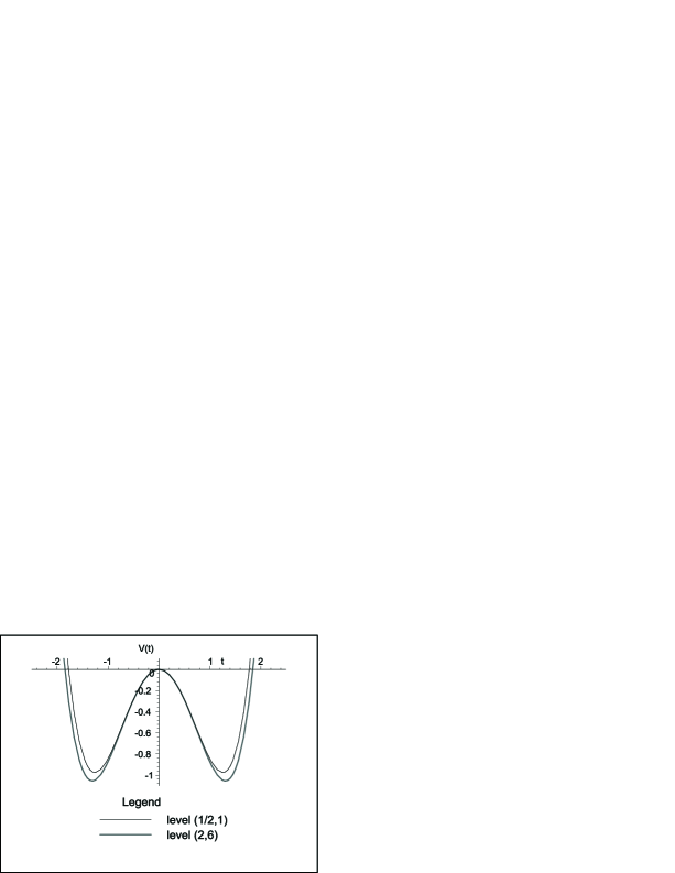
Figure 3: Graphics of the tachyon potential at the levels $(1/2,\,1)$ and $(2,\,6)$. “$-1$” is equal to the minus tension of non BPS D$p$-brane $\tilde{\tau}_{p}=\frac{2}{\pi^{2}g^{2}_{o}\alpha^{\,\prime\,\frac{p+1}{2}}}$.

$$\begin{split}\mathcal{V}_{\mathrm{eff}}^{(\frac{1}{2},\,1)}(t)&=\frac{\pi^{2}\tilde{\tau}_{p}}{2}\left[\frac{81}{1024}t^{4}-\frac{1}{4}t^{2}\right],\\ \mathcal{V}_{\mathrm{eff}}^{(2,\,6)}(t)&=\frac{\pi^{2}\tilde{\tau}_{p}}{2}\left[\frac{5053}{69120}t^{4}-\frac{1}{4}t^{2}\right]\end{split}$$ (4.12)

The critical points of these functions are collected in Table 3.

Potential	Critical points	Critical values
$\mathcal{V}_{\mathrm{eff}}^{(\frac{1}{2},\,1)}$	$t_{c}=0$	$\mathcal{V}_{c}=0$
	$t_{c}=\pm\frac{8\sqrt{2}}{9}\approx\pm 1.257$	$\mathcal{V}_{c}\approx-0.975\tilde{\tau}_{p}$
$\mathcal{V}_{\mathrm{eff}}^{(2,\,6)}$	$t_{c}=0$	$\mathcal{V}_{c}=0$
	$t_{c}=\pm\frac{24}{5053}\sqrt{75795}\approx\pm 1.308$	$\mathcal{V}_{c}\approx-1.058\tilde{\tau}_{p}$

Table 3: The critical points of the tachyon potential at levels $(1/2,\,1)$ and $(2,\,6)$.

One sees that the potential has a global minimum and the value of this minimum is $97.5\%$ at level $(1/2,\,1)$ and $105.8\%$ at level $(2,\,6)$ of the tension $\tilde{\tau}_{p}$ of the non-BPS $\mathrm{D}p$-brane.

5 Conclusion

We have computed the effective tachyon potential for non-BPS-$\mathrm{D}$-brane in cubic SSFT on two first nontrivial levels. The essential feature of our scheme is the choice of the $0$ picture for the string field in contrast to the $-1$ picture [13]. This choice of the picture enlarge the set of space-time fields involved into the calculation at any level. It is interesting to note that already at the first level the value of the potential at minimum is $97.5\%$ of brane’s tension. At the next nontrivial level we use the special gauge (3.4), which dramatically simplifies the computations of the tachyon potential. The validity of this gauge will be the subject of forthcoming publication [28].

In conclusion, our scheme confirms the existence of the minimum as it was predicted by Sen’s conjecture, and gives $97.5\%$ of brane’s tension at the first step and $105.8\%$ at the second. Hence, we see that the level truncation scheme does not provide monotone convergence in this gauge.

Appendix A Notations

Here we collect notations we use in our calculations (for more details see [15]).

Table 4: Notations, correlation functions and OPE-s.

$X_{L}^{\mu}(z)X_{L}^{\nu}(w)\sim-\frac{\alpha^{\prime}}{2}\eta^{\mu\nu}\log(z-w)$	$\partial X^{\mu}(z)\partial X^{\nu}(w)\sim-\frac{\alpha^{\,\prime}}{2}\eta^{\mu\nu}\frac{1}{(z-w)^{2}}$
$\psi^{\mu}(z)\psi^{\nu}(w)\sim-\frac{\alpha^{\prime}}{2}\eta^{\mu\nu}\frac{1}{z-w}$
$c(z)b(w)\sim b(z)c(w)\sim\frac{1}{z-w}$	$\gamma(z)\beta(w)\sim-\beta(z)\gamma(w)\sim\frac{1}{z-w}$
$\phi(z)\phi(w)\sim-\log(z-w)$	$\xi(z)\eta(w)\sim\eta(z)\xi(w)\sim\frac{1}{z-w}$
$\langle c(z_{1})c(z_{2})c(z_{3})\rangle=(z_{1}-z_{2})(z_{2}-z_{3})(z_{3}-z_{1}){}{}{}{}$	$\langle e^{-2\phi(y)}\rangle=1$
$\left\langle e^{i2p_{\alpha}X_{L}^{\alpha}(y)-i2b_{i}X_{L}^{i}(y)}e^{i2k_{\beta}X_{L}^{\beta}(z)+i2b_{j}X_{L}^{j}(z)}\right\rangle=(2\pi)^{p+1}\alpha^{\,\prime-\frac{p+1}{2}}\delta(p+k)(y-z)^{2\alpha^{\,\prime}(k^{2}+b^{2})}$
$T_{B}=-\frac{1}{\alpha^{\,\prime}}\partial X\cdot\partial X-\frac{1}{\alpha^{\,\prime}}\partial\psi\cdot\psi$	$T_{F}=-\frac{1}{\alpha^{\,\prime}}\partial X\cdot\psi$
$T_{bc}=-2b\partial c-\partial bc$	$T_{\beta\gamma}=-\frac{3}{2}\beta\partial\gamma-\frac{1}{2}\partial\beta\gamma$
$T_{\phi}=-\frac{1}{2}\partial\phi\partial\phi-\partial^{2}\phi$	$T_{\eta\xi}=\partial\xi\eta$
$T_{B}(z)T_{B}(w)\sim\frac{15}{2(z-w)^{4}}+\frac{2}{(z-w)^{2}}T_{B}(w)+\frac{1}{z-w}\partial T_{B}(w)$
$T_{B}(z)T_{F}(w)\sim\frac{3/2}{(z-w)^{2}}T_{F}(w)+\frac{1}{z-w}\partial T_{F}(w)$
$T_{F}(z)T_{F}(w)\sim\frac{5/2}{(z-w)^{3}}+\frac{1/2}{z-w}T_{B}(w)$
$\gamma=\eta e^{\phi}$	$\beta=e^{-\phi}\partial\xi$
$T_{\beta\gamma}=T_{\phi}+T_{\eta\xi}$	$\gamma^{2}=\eta\partial\eta e^{2\phi}$
$\phi-\text{charge:}\quad\left[\frac{1}{2\pi i}\oint d\zeta\partial\phi(\zeta),\,\mathcal{A}_{q}\right]=q\mathcal{A}_{q}$
$Q_{B}=\frac{1}{2\pi i}\oint d\zeta\,\left[c(T_{B}+T_{\beta\gamma}+\frac{1}{2}T_{bc})+\frac{1}{\alpha^{\,\prime}}\gamma\psi\cdot\partial X-\frac{1}{4}b\gamma^{2}\right]$
$Q_{B}=\frac{1}{2\pi i}\oint d\zeta\,\left[c(T_{B}+T_{\phi}+T_{\eta\xi}+\frac{1}{2}T_{bc})+\frac{1}{\alpha^{\,\prime}}\eta e^{\phi}\psi\cdot\partial X+\frac{1}{4}b\partial\eta\eta e^{2\phi}\right]$
$\mathrm{X}=\frac{1}{\alpha^{\,\prime}}e^{\phi}\psi\cdot\partial X+c\partial\xi+\frac{1}{4}b\partial\eta e^{2\phi}+\frac{1}{4}\partial(b\eta e^{2\phi})$
$Y=4c\partial\xi e^{-2\phi}$

Appendix B Cyclicity Property

The proof of the cyclicity property is very similar to the one given in [13]. But there is one specific point — insertion of the double step inverse picture changing operator $Y_{-2}$ (2.8). So we repeat the proof with all necessary modifications.

Let $T_{n}$ and $R$ denotes rotation by $-\frac{2\pi}{n}$ and $-2\pi$ respectively:

$$T_{n}(w)=e^{-\frac{2\pi i}{n}}w,\qquad R(w)=e^{-2\pi i}w.$$

These transformations have two fixed points namely $0$ and $\infty$. Let us apply the transformation $T_{n}$ to the maps $f^{(n)}_{k}$ (2.10) and we get the identities:

$$T_{n}\circ f_{k}^{(n)}=f_{k+1}^{(n)},\quad k<n,\qquad T_{n}\circ f_{n}^{(n)}=R\circ f_{1}^{(n)},\qquad n=2,3.$$ (B.1)

Since the weight of the operator $Y_{-2}$ is zero and $0$ and $\infty$ are fixed points of $T_{n}$ and $R$, the operator $Y_{-2}$ remains unchanged. Due to $SL(2,\mathbb{R})$-invariance of the correlation function we can write down a chain of equalities

$$\langle Y_{-2}\,F_{1}^{(n)}\circ A_{1}\dots F_{n-1}^{(n)}\circ A_{n-1}F_{n}^{(n)}\circ\mathcal{O}_{h}\rangle=\langle Y_{-2}\,f_{1}^{(n)}\circ A_{1}\dots f_{n-1}^{(n)}\circ A_{n-1}f_{n}^{(n)}\circ\mathcal{O}_{h}\rangle\\ =\langle Y_{-2}\,T_{n}\circ f_{1}^{(n)}\circ A_{1}\dots T_{n}\circ f_{n-1}^{(n)}\circ A_{n-1}T_{n}\circ f_{n}^{(n)}\circ\mathcal{O}_{h}\rangle\\ =e^{-2\pi ih}\langle Y_{-2}\,F_{1}^{(n)}\circ\mathcal{O}_{h}\,F_{2}^{(n)}\circ A_{1}\dots F_{n}^{(n)}\circ A_{n-1}\rangle.$$ (B.2)

In the last line we assume that $\mathcal{O}_{h}$ is a primary field of weight $h$ and use the transformation law of primary fields under rotation:

$$(R\circ\mathcal{O}_{h})(w)=e^{-2\pi ih}\mathcal{O}_{h}(e^{-2\pi i}w).$$

Also we change the order of operators in correlation function without change of a sign, because the expression inside the brackets should be odd (otherwise it will be equal to zero) and therefore no matter whether $\Phi$ odd or even. So the cyclicity property reads

$$\langle\!\langle Y_{-2}|A_{1},\dots,A_{n}\rangle\!\rangle=e^{-2\pi ih_{n}}\langle\!\langle Y_{-2}|A_{n},A_{1},\dots,A_{n-1}\rangle\!\rangle$$ (B.3)

Examples. Now we consider some applications of the cyclicity property (B.3). GSO$+$ sector consists of the fields with integer weights and therefore their exponential factor is equal to $1$, while GSO$-$ sector consists of the fields with half integer weights and therefore their exponential factor is $-1$. Now we give few examples

$$\langle\!\langle Y_{-2}|\mathcal{A}_{+},Q_{B}\mathcal{A}_{+}\rangle\!\rangle =\langle\!\langle Y_{-2}|Q_{B}\mathcal{A}_{+},\mathcal{A}_{+}\rangle\!\rangle,$$ (B.4a)

$$\langle\!\langle Y_{-2}|\mathcal{A}_{-},Q_{B}\mathcal{A}_{-}\rangle\!\rangle =-\langle\!\langle Y_{-2}|Q_{B}\mathcal{A}_{-},\mathcal{A}_{-}\rangle\!\rangle,$$ (B.4b)

$$\langle\!\langle Y_{-2}|\mathcal{A}_{+},\mathcal{A}_{-},\mathcal{A}_{-}\rangle\!\rangle =-\langle\!\langle Y_{-2}|\mathcal{A}_{-},\mathcal{A}_{+},\mathcal{A}_{-}\rangle\!\rangle=\langle\!\langle Y_{-2}|\mathcal{A}_{-},\mathcal{A}_{-},\mathcal{A}_{+}\rangle\!\rangle.$$ (B.4c)

Appendix C Twist Symmetry

The proof of the twist symmetry is similar to the one given in [13]. But there is one specific point — insertion of the operator $Y_{-2}$. So we repeat this proof here with all necessary modifications.

A twist symmetry is a relation between correlation functions of operators written in one order and in the inverse one:

$$\langle\!\langle Y_{-2}|\mathcal{O}_{1},\dots,\mathcal{O}_{n}\rangle\!\rangle=(-1)^{?}\langle\!\langle Y_{-2}|\mathcal{O}_{n},\dots,\mathcal{O}_{1}\rangle\!\rangle.$$ (C.1)

We are interesting in this relation for $n=3$.

1) Let us consider the following transformations $M(w)=e^{-i\pi}w$ and $\tilde{I}(w)=e^{i0}/w$. The transformation $\tilde{I}$ has the following properties:

$$\tilde{I}(z_{1})\tilde{I}(z_{2})=\tilde{I}(z_{1}z_{2})\quad\text{and}\quad\tilde{I}(z^{2/3})=(\tilde{I}(z))^{2/3}.$$

The pair of points $0$ and $\infty$ is not affected by $M$ and $\tilde{I}$, therefore the double-step inverse picture changing operator $Y_{-2}$ remains unchanged. For the maps (2.10) we have got the following composition laws

$$f_{1}^{(3)}\circ M=\tilde{I}\circ f_{1}^{(3)},\quad f_{2}^{(3)}\circ M=\tilde{I}\circ f_{3}^{(3)}\quad\text{and}\quad f_{3}^{(3)}\circ M=\tilde{I}\circ f_{2}^{(3)}.$$ (C.2)

2) Since there is an identity $M\circ\mathcal{O}(0)=e^{-i\pi h}\mathcal{O}(0)$ we can apply it to (C.1)

$$\langle\!\langle Y_{-2}|\mathcal{O}_{1},\mathcal{O}_{2},\mathcal{O}_{3}\rangle\!\rangle=e^{i\pi\sum h_{j}}\langle Y_{-2}\,f_{1}^{(3)}\circ M\circ\mathcal{O}_{1}\,f_{2}^{(3)}\circ M\circ\mathcal{O}_{2}\,f_{3}^{(3)}\circ M\circ\mathcal{O}_{3}\rangle\\ =e^{i\pi\sum h_{j}}\langle Y_{-2}\,\tilde{I}\circ f_{3}^{(3)}\circ\mathcal{O}_{1}\,\tilde{I}\circ f_{2}^{(3)}\circ\mathcal{O}_{2}\,\tilde{I}\circ f_{1}^{(3)}\circ\mathcal{O}_{3}\rangle\\ =e^{i\pi\sum h_{j}}\langle Y_{-2}\,f_{3}^{(3)}\circ\mathcal{O}_{1}\,f_{2}^{(3)}\circ\mathcal{O}_{2}\,f_{1}^{(3)}\circ\mathcal{O}_{3}\rangle$$ (C.3)

in the last line we use the invariance with respect to $SL(2,\mathbb{R})$. Let $N_{odd}$ and $N_{even}$ be a number of odd or even respectively fields in the set $\{\mathcal{O}_{1},\mathcal{O}_{2},\mathcal{O}_{3}\}$. After rearranging the fields one gets

$$\langle\!\langle Y_{-2}|\mathcal{O}_{1},\mathcal{O}_{2},\mathcal{O}_{3}\rangle\!\rangle=e^{i\pi\sum h_{j}}(-1)^{\frac{N_{odd}\left(N_{odd}-1\right)}{2}}\langle\!\langle Y_{-2}|\mathcal{O}_{3},\mathcal{O}_{2},\mathcal{O}_{1}\rangle\!\rangle.$$ (C.4)

3) Since the correlation function is non zero only for odd expression, number $N_{odd}$ is odd and $N_{odd}=2m+1$ for some integer $m$. Also we have an identity $N_{even}+N_{odd}=3$. It’s not difficult to check that

$$(-1)^{\frac{N_{odd}\left(N_{odd}-1\right)}{2}}=(-1)^{m}=(-1)^{\frac{N_{odd}-1}{2}+\frac{N_{odd}+N_{even}-3}{2}}=(-1)^{N_{odd}+\frac{N_{even}}{2}}.$$ (C.5)

Combining (C.4) and (C.5) we get the twist property

$$\begin{split}\langle\!\langle Y_{-2}|\mathcal{O}_{1},\mathcal{O}_{2},\mathcal{O}_{3}\rangle\!\rangle&=\Omega_{1}\Omega_{2}\Omega_{3}\,\langle\!\langle Y_{-2}|\mathcal{O}_{3},\mathcal{O}_{2},\mathcal{O}_{1}\rangle\!\rangle,\\ \mbox{where}\quad\Omega_{j}&=\left\{\begin{tabular}[]{LL}(-1)^{h_{j}+1},&h_{j}\in\mathbb{Z}\quad\mbox{ (i.e. GSO$+$)}\\ (-1)^{h_{j}+\frac{1}{2}},&h_{j}\in\mathbb{Z}+\frac{1}{2}\quad\mbox{ (i.e. GSO$-$)}.\end{tabular}\right.\end{split}$$ (C.6)

Examples.

$i)$ Let $A_{+}=A_{1}+A_{2}$. Each term in

$$A_{+}^{3}=A_{1}^{3}+(A_{1}A_{2}^{2}+A_{2}^{2}A_{1})+A_{2}A_{1}A_{2}+(A_{2}^{2}A_{1}+A_{1}A_{2}^{2})+A_{1}A_{2}A_{1}+A_{2}^{3}$$

should be twist invariant to be nonzero. Therefore we get $\Omega_{1}=1$ and $\Omega_{2}=1$.

$ii)$ Let we have fields $A_{+}$ and $A_{-}=a_{1}+a_{2}$. Using cyclicity property (B.4) one gets

$$2(A_{+},a_{1}+a_{2},a_{1}+a_{2})=(A_{+}a_{1}^{2}+a_{1}^{2}A_{+})+(A_{+}a_{2}^{2}+a_{2}^{2}A_{+})+(A_{+}a_{1}a_{2}+a_{2}a_{1}A_{+})+(A_{+}a_{2}a_{1}+a_{1}a_{2}A_{+}).$$

So we get $\Omega_{+}=1$ and $\Omega_{+}\Omega_{1}\Omega_{2}=1$. If $\Omega_{1}=1$ (tachyon’s sector) then $\Omega_{2}=1$ too. Therefore we can consider a sector with $\Omega=1$ only.

References

-
[1]
E. Witten,
Noncommutative geometry and string field theory,
Nucl. Phys. B268 (1986), 253.
E. Witten, Noncommutative Geometry and String Field Theory, Nucl. Phys. B207 (1988), p.169 - [2] E.Witten, Interacting field theory of open superstrings, Nucl. Phys. B276 (1986) 291.
-
[3]
V.A.Kostelecky and S.Samuel, The static
tachyon potential n the open bosonic string theory, Phys.Lett.
B207 (1988), p.169.
V.A.Kostelecky and S.Samuel, The tachyon potential in string theory, DPF Conf. pp.813–816 (1988)
V.A.Kostelecky and S.Samuel, On a nonperturbative vacuum for the open bosonic string, Nucl.Phys. (1990) B336, p.286 - [4] I.Ya.Aref’eva, P.B.Medvedev and A.P.Zubarev, Nonperturbative vacuum for superstring field theory and supersymmetry breaking,Mod.Phys.Lett. A6, pp.949-958 (1991)
- [5] I.A. Aref’eva, P.B. Medvedev and A.P. Zubarev, Background formalism for superstring field theory, Phys.Lett. B240, pp.356–362 (1990)
- [6] C.R. Preitschopf, C.B. Thorn and S.A. Yost, Superstring Field Theory,UFIFT–HEP–89–19
- [7] I.Ya.Aref’eva, P.B.Medvedev and A.P.Zubarev, New representation for string field solves the consistency problem for open superstring field, Nucl.Phys. B341, pp.464–498 (1990)
-
[8]
A. Sen,
Stable non BPS bound states of bps d-branes,
JHEP 08, 010 (1998), hep-th/9805019
A. Sen, SO(32) spinors of type i and other solitons on brane - anti-brane pair, JHEP 09, 023 (1998), hep-th/9808141 - [9] A. Sen, B. Zwiebach, Tachyon condensation in string field theory, JHEP 0003 (2000) 002, hep-th/9912249.
- [10] N.Moeller, W.Taylor, Level truncation and the tachyon in open bosonic string field theory, Nucl.Phys. B583 (2000) 105-144, hep-th/0002237
- [11] N.Berkovits, Super-poincare invariant superstring field theory, Nucl.Phys. B450 (1995) 90, hep-th/9503099
- [12] N. Berkovits, The Tachyon Potential in Open Neveu-Schwarz String Field Theory, JHEP 0004 (2000) 022, hep-th/0001084.
- [13] N. Berkovits, A. Sen, B. Zwiebach, Tachyon Condensation in Superstring Field Theory, hep-th/0002211.
- [14] P. De Smet, J. Raeymaekers, Level Four Approximation to the Tachyon Potential in Superstring Field Theory, JHEP 0005 (2000) 051, hep-th/0003220.
- [15] D. Friedan, E. Martinec, and S. Shenker, Conformal Invariance, Supersymmetry, and String Theory, Nucl. Phys. B271 (1986) 93.
- [16] M.V.Green, N.Sieberg, Contact interactions in superstring theory, Nucl. Phys. B299 (1988) 559.
- [17] J.Greensite, F.R.Klinkhamer, Superstring scattering amplitudes and contact interactions, Nucl. Phys. B304 (1988) 108.
- [18] I.Ya.Aref’eva, P.B.Medvedev, Anomalies in Witten’s field theory of the NSR string, Phys.Lett. B212, 3, p.299 (1988)
- [19] C. Wendt, Scattering amplitudes and contact interactions in Witten’s superstring field theory, Nucl. Phys. B314 (1989), p.209
- [20] B.V. Urosevic, A.P. Zubarev, On the component analysis of modified superstring field theory actions, Phys.Lett. B246, pp.391-398 (1990)
- [21] A. LeClair, M.E. Peskin and C.R. Preitschopf, String field theory on the conformal plane, Nucl. Phys. B317 (1989)
- [22] J. Polchinski, Introduction to Superstrings, Vol I and II
- [23] A. Sen, Non-BPS States and Branes in String Theory, hep-th/9904207, MRI-PHY/P990411
- [24] P. De Smet, J. Raeymaekers, The Tachyon Potential in Witten‘s Superstring Field Theory, hep-th/0004112.
- [25] A. Bilal, M(atrix) theory: a pedagogical introduction, hep-th/9710136
- [26] A.Sen, Universality of the Tachyon Potential, hep-th/9911116, JHEP 9912 (1999) 027
- [27] A. Iqbal, A. Naqvi, Tachyon Condensation on a non-BPS D-brane, hep-th/0004015.
- [28] I. Ya. Arefeva, D. M. Belov, A. S. Koshelev and P. B. Medvedev, Work in progress