A new family of non critical bosonic string backgrounds in arbitrary space time dimension $D$ and with $ISO(1,D-2)$ Poincaré invariance are presented. The metric warping factor and dilaton agree asymptotically with the linear dilaton background. The closed string tachyon equation of motion enjoys, in the linear approximation, an exact solution of “kink” type interpolating between different expectation values. A renormalization group flow interpretation ,based on a closed string tachyon potential of type $-T^{2}e^{-T}$, is suggested.

1 Introduction and Summary

In order for strings to behave as consistent quantum systems, a mimimal requirement seems to be the absence of anomalies.

World sheet conformal invariance at tree level in the string perturbative expansion leads to vanishing sigma model beta functions. Denoting $D$ the dimension of the target space-time the relevant beta functions for the bosonic string are

$$\beta^{g}_{AB} =\alpha^{\prime}R_{AB}+2\alpha^{\prime}\nabla_{A}\nabla_{B}\Phi-\frac{\alpha^{\prime}}{4}H_{ACD}H_{B}^{CD}+o(\alpha^{\prime 2})$$

$$\beta^{b}_{AB} =-\frac{\alpha^{\prime}}{2}\nabla^{D}H_{DAB}+\alpha^{\prime}\nabla^{D}\Phi H_{DAB}+o(\alpha^{\prime 2})$$

$$\beta^{\Phi} =\frac{D-26}{6}-\frac{\alpha^{\prime}}{2}\nabla^{2}\Phi+\alpha^{\prime}\nabla_{D}\Phi\nabla^{D}\Phi-\frac{\alpha^{\prime}}{24}H_{ABC}H^{ABC}+o(\alpha^{\prime 2})$$ (1)

The simplest solution is of course the critical string $D=26$ in flat Minkowski space time with constant dilaton and vanishing antisymmetric tensor. Another well known solution in $D\neq 26$ is the linear dilaton background [9]

$$\Phi=q_{\mu}X^{\mu}$$ (2)

in flat $D$ dimensional Minkowski space-time, with

$$q_{\mu}q^{\mu}=\frac{26-D}{6\alpha^{\prime}}$$ (3)

The linear dilaton background solution is exact to all orders in $\alpha^{\prime}$ and defines a good conformal field theory. Moreover for $D$ smaller or equal to two this background is tachyon free in the linear approximation, and is believed to develop a tachyonic barrier that prevents strings to enter in the string strong coupling region.

Motivated by the curved Liouville approach of Polyakov [11] to non critical backgrounds we will present in this letter a new family of solutions to the sigma model beta function equations, at first order in $\alpha^{\prime}$, for generic values of $D$ and with $ISO(1,D-2)$ Poincare invariance

$$ds^{2}=a(r)d\vec{x}_{1,D-2}^{2}+dr^{2}$$ (4)

Backgrounds of this type are typical in the holographic context once we identify the coordinate $r$ with the holographic direction or in curved Liouville if we interpret $r$ as the extra Liouville direction.

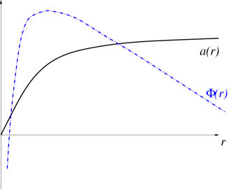
Figure 1: Warp factor and dilaton v.s. holographic coordinate. In the $r\rightarrow\infty$ linear dilaton behavior in flat Minkowski space time can be noticed.

To be specific, we shall find ( see Figure 1) that in $D=5$ spacetime dimensions (corresponding to one holographic plus the ordinary four minkowskian ones), the warp factor is:

$$a(r)=th(\sqrt{\frac{21}{6\alpha^{\prime}}}r)$$ (5)

and the dilaton

$$\Phi=\frac{1}{2}\log\left[th(\sqrt{\frac{21}{6\alpha^{\prime}}}r)\frac{1}{cosh^{2}(\sqrt{\frac{21}{6\alpha^{\prime}}}r)}\right]$$ (6)

Notice from equations (5) and (6) that this solution in the asymptotic region $r\rightarrow\infty$ coincides with flat Minkowski space-time with the appropiated linear dilaton background. At $r=0$ the warp factor goes to zero inducing a naked singularity. Close to the origin we reproduce the metric of reference [2] with a logaritmic behavior for the dilaton. Moreover in the limit $\alpha^{\prime}\rightarrow 0$ the metric becomes flat Minkowski except in a neighborhood of the origin .

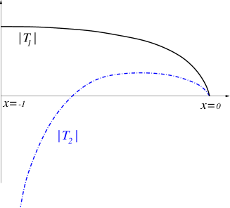
Figure 2: The solid line represents the kink solution interpolating between $T=0$ at $x=0,(r=\infty)$ and $T=cte$ at $x=-1,(r=0)$. The variable $x$ is defined in equation (3.2.2).

With respect to the problem of the tachyon stability we study the tachyon equation of motion in the linear approximation. The equation of motion becomes Riemann’s equation with three singular points. In the asymptotic region $r\rightarrow\infty$ we find the familiar $c=1$ barrier for linear dilaton background; namely for $D>2$ the tachyon goes to zero oscillating. At the origin the exact solution, preserving energy conservation, goes to a constant. Thus this solution can be temptatively interpreted as a kind of tachyonic kink ( see Fig 2) interpolating - in the sense of a renormalization group flow- the unstable linear dilaton asymptotic regime with vanishing vacuum expectation value of the tachyon and a stable background characterized by a non vanishing tachyon vacuum expectation value. This interpretation could be probably supported by a closed string tachyon potential of type $V(T)=-e^{-T}T^{2}$ as recently suggested in reference [13]. In the rest of this paper we will present the technical details of our analysis.

2 A new family of non-critical bosonic string backgrounds

For vanishing Kalb-Ramond field the beta function equation $\beta^{g}=0$ for the Poincare invariant metric (4) reads:

$$\frac{2aa^{\prime\prime}+(d-2)(a^{\prime})^{2}}{4a}\eta_{\mu\nu} =a^{\prime}\Phi^{\prime}\eta_{\mu\nu}$$

$$\frac{d}{4}\frac{2aa^{\prime\prime}-(a^{\prime})^{2}}{a^{2}} =2\Phi^{\prime\prime}$$ (7)

for $d=D-1$. The dilaton solving the first of these equations is given by

$$\Phi=\frac{1}{2}\ log\,a^{\prime}+\frac{d-2}{4}log\,a$$ (8)

and the general solution for the metric factor would be obtained by integrating the following equation:

$$\frac{da}{dr}=c_{1}a^{1+\frac{\sqrt{d}}{2}}+c_{2}a^{1-\frac{\sqrt{d}}{2}}$$ (9)

There are now several possibilities:

• $c_{1}c_{2}<0$. The solution then reduces to:

  $$a(r)=\left[\frac{\sqrt{-c_{1}c_{2}}}{c_{1}}th\left(\sqrt{-c_{1}c_{2}}\frac{\sqrt{d}}{2}(r+c_{3})\right)\right]^{\frac{2}{\sqrt{d}}}$$ (10)

• $c_{1}c_{2}>0$. The solution reads :

  $$a(r)=\left[\frac{\sqrt{c_{1}c_{2}}}{c_{1}}tg\left(\sqrt{c_{1}c_{2}}\frac{\sqrt{d}}{2}(r+c_{3})\right)\right]^{\frac{2}{\sqrt{d}}}$$ (11)

• $c_{2}=0$. The solution is then:

  $$a(r)=(r+c_{3})^{-\frac{2}{\sqrt{d}}}$$ (12)

  (This is the dual $r\to\frac{1}{r}$ of the solution presented in [2]).

• $c_{1}=0$. This leads to:

  $$a(r)=(r+c_{3})^{\frac{2}{\sqrt{d}}}$$ (13)

  (This is the confining background introduced in [2]).

• $c_{1}=c_{2}=0$. This is the linear dilaton solution:

  $$a =a_{0}$$

  $$\Phi =c_{3}+c_{4}r$$ (14)

  with $c_{3},c_{4}$ arbitrary constants. Notice that in this case equations (2) imply $\Phi^{\prime\prime}=0$.

The most important thing about this family of solutions is that they are non-critical; that is, if we compute the beta function of the dilaton (which is guaranteed to be a constant by virtue of the first two equations and Bianchi identities for the spacetime curvature,) it so happens that

$$c_{1}c_{2}=\frac{4}{6\alpha^{\prime}}(1-\frac{25}{d})$$ (15)

This clearly means that if $c_{1}c_{2}<0$, there is a solution in the family for any $D<26$; whereas for $c_{1}c_{2}>0$ the solution exists for any $D>26$.

It is also worth remarking that as soon as one of the two arbitrary constants vanish, the solution must necessarily become critical (that is, with $D=26$).

Let us now briefly describe some properties of the solutions in the physically most interesting case, namely for $D<26$. The behavior in the asymptotic region $r\rightarrow\infty$ for the metric factor $a$ is

$$a\rightarrow\bar{a}=(\frac{-c_{2}}{c_{1}})^{\frac{1}{\sqrt{d}}}$$ (16)

whereas the dilaton yields

$$\Phi\rightarrow-\sqrt{\frac{25-d}{6\alpha^{\prime}}}r$$ (17)

where we easily recognize the precise behavior of the linear dilaton solution in flat space-time.

In the region $r\rightarrow 0$ we get instead

$$a\rightarrow\left({\frac{c_{2}\sqrt{d}}{2}}r\right)^{\frac{2}{\sqrt{d}}}$$ (18)

and the dilaton goes as

$$\Phi\rightarrow(\sqrt{d}-1)\log r$$ (19)

Notice that all these solutions are singular at $r=0$. For instance the scalar curvature in d=4 is given by

$$R={-c_{1}c_{2}}\frac{(a^{2}-1)(9a^{2}-1)}{a^{2}}$$ (20)

Given the fact that this is the general  solution with our ansatz, this means that the existence of the naked singularity is somewhat embodied in the ansatz itself.

A simple generalization of this background (4) can be obtained by adding a certain number $d^{\prime}$ of extra flat dimensions $(D=d+d^{\prime}+1)$:

$$ds^{2}=a(r)d\vec{x}_{1,d}^{2}+dr^{2}+d\vec{y}_{d^{\prime}}$$ (21)

The only change in this case is on the values of the constants $c_{1},c_{2}$ that are now fixed by the relation

$$\frac{dc_{1}c_{2}}{4}=\frac{(d+d^{\prime}-25)}{6\alpha^{\prime}}$$ (22)

3 Closed String Tachyons

Bosonic string backgrounds suffer from an intrinsic source for instability (which sometimes has been taken as an indication of the existence of another, physically interesting and energetically favoured vacuum [5]), namely, a tachyonic scalar excitation in the closed string sector with

$$m^{2}=-\frac{4}{\alpha^{\prime}}.$$ (23)

It was first suggested by Polyakov [11] that in a metric of type (4) the tachyon unstability could be tamed leading to a peaceful condensation. In addition we know that in a non trivial space time - AdS is a good example [4] - normalizability and energy conservation imposses strong restrictions on the allowed spectrum of masses. Following this last approach the first thing we will do would be to derive from energy conservation and normalizability, the boundary conditions on field configurations. Next we will consider - in the linear approximation - the exact solution to the tachyon equation of motion satisfying these boundary conditions. Finally we will interpret the solution as a kink describing tachyon condensation.

3.1 Boundary Conditions

3.1.1 Normalization

First of all, if the scalar is complex, there is a conserved number current:

$$N^{A}\equiv e^{-2\Phi}((f_{2})^{*}\partial^{A}f_{1}-f_{1}\partial^{A}(f_{2})^{*})$$ (24)

which gives rise to a conserved particle number

$$N\equiv\int d^{d-1}xdr\sqrt{g}e^{-2\Phi}(f^{*}\partial^{0}f-f\partial^{0}f^{*})$$ (25)

when this integral converges. The $a$-dependent factors in the measure behave as:

$$N\sim a^{(d-1)/2}\frac{1}{a^{\prime}a^{\frac{d-2}{2}}}$$ (26)

In the generic case, for $c_{1}c_{2}<0$ this behaves for $a\sim 0$ as:

$$N\sim a^{\frac{\sqrt{d}-1}{2}}$$ (27)

On the other hand, when $a$ reached its asymptotic value, $a\rightarrow\bar{a}$,

$$N\sim\frac{1}{\bar{a}-a}$$ (28)

This last behaviour selects functions that vanish as a power when $a\rightarrow\bar{a}$. That is,

$$lim_{a\rightarrow\bar{a}}f=(\bar{a}-a)^{\delta}$$ (29)

where $\delta>\frac{1}{2}$.

3.1.2 The definition of Conserved Energy

Given an arbitrary scalar field with energy-momentum tensor $T_{AB}$, there is a Killing energy current, namely

$$j^{A}\equiv T^{AB}k_{B}$$ (30)

which is covariantly conserved,

i.e.

$$\nabla_{A}j^{A}=0$$ (31)

In our case, the Killing corresponding to temporal translations is:

$$k\equiv\frac{\partial}{\partial t}$$ (32)

Applying Stokes’theorem to the integral over the $(d+1)$-dimensional region $\mathcal{R}$ defined in terms of a large distance $L$ by $t_{0}<t<t_{1}$,and by $-L<x^{i}<L$,($i,j,\ldots=1,\ldots d-1$), $0<r<L$, of the $(d+1)$-form proportional to the first member of (31), i.e. of $d*j$, where $j$ is the one-form dual to the current, $j\equiv j_{A}dx^{A}$, we get

$$0=\int_{\mathcal{M}}d*j=\int_{\partial\mathcal{M}}*j=E(t_{2})-E(t_{1})+\Delta E$$ (33)

where

$$E(t)\equiv\int d^{(d-1)}xdr\sqrt{g}j^{0}(t,x^{i},r)$$ (34)

and the flux over the boundary $\partial M$,

$$\Delta E=(\int_{x^{i}=L}-\int_{x^{i}=-L})(\sqrt{g})(\epsilon_{ii_{1}\ldots i_{d-2}}dt\wedge dx^{i_{1}}\wedge\ldots\wedge dx^{i_{d-2}}\wedge dr)j^{i}+(\int_{r=L}-\int_{r=0})d^{d}x(\sqrt{g})j^{d}.$$ (35)

Only when the physical boundary conditions are such that

$$\Delta E=0$$ (36)

there is actual energy conservation,

$$\frac{dE}{dt}=0$$ (37)

For a scalar field of mass $m$ it is readily found that

$$T_{AB}=\frac{1}{2}e^{-2\Phi}[\nabla_{A}\phi\nabla_{B}\phi-\frac{1}{2}g_{AB}(g^{CD}\nabla_{C}\phi\nabla_{D}\phi-m^{2}\phi^{2})]$$ (38)

so that the $(d+1)$-dimensional energy is:

$$E[\phi]\equiv\frac{1}{4}\int d^{(d-1)}xdr\sqrt{g}T^{0}_{B}k^{B},$$ (39)

i.e.,denoting the scalar perturbation by $T$,

$$E=\int drd^{d-1}x\frac{1}{\sqrt{a}a^{\prime}}\left[\dot{T}^{2}+(\nabla_{d-1}T)^{2}+a((\partial_{r}T)^{2}+m^{2}T^{2})\right]$$ (40)

In all cases the important thing is the behaviour of the flux at the singular boundary, which in turn is dominated by the behaviour of $j^{d}$, when $a\rightarrow 0$, namely

$$j^{d}\sim-\frac{a}{2}\frac{1}{a^{\prime}a^{\frac{d-2}{2}}}\frac{1}{a}\partial_{r}T\dot{T}=-\frac{1}{2}a^{1-\frac{d}{2}}T^{\prime}\dot{T}$$ (41)

3.1.3 Positive-definiteness

Combining the results of the preceding two paragraphs we can read the conditions for the scalar perturbations to be normalizable, as well as enjoy a conserved energy, that is,

$$f \sim_{a=0}0(a^{-u})$$

$$f \sim_{a=\bar{a}}(\bar{a}-a)^{v}$$ (42)

with $0<u<1$ and $v>\frac{1}{2}$.

If we want moreover the now well defined energy to be finite it is clearly necessary (owing to the $a^{\prime}$ factor in the denominator) that when $r\rightarrow\infty$

$$T\sim e^{-\mu^{2}r}$$ (43)

with

$$\mu^{2}>\sqrt{\frac{25-d}{6\alpha^{\prime}}}$$ (44)

which is much faster that required by (3.1.3).We can define another functional space in which energy is not only conserved, but also finite, and this space is essentially characterized by the behavior (44).

It is then plain that in the conserved-energy functional space defined by (3.1.3) there are fluctuations with arbitarily large negative energy, namely all those that at infinity behave as (43) with $|\mu|<|m|$. In the more restrictive finite-energy space (44), this behavior still persists as long as $d>1$. This is the same bound found for the linear dilaton background.

3.2 The tachyon equation

Let us now examine the space of solutions of the linearized equation of motion and check whether on shell there are elements of our functional space of well-defined fluctuations.

We shall write the wave equations (following the conventions of [10]) as:

$$\nabla^{2}T-2\nabla^{A}\Phi\nabla_{A}T-m^{2}T=0$$ (45)

For the Poincaré invariant ansatz the dilaton is given by

$$\Phi=\frac{1}{2}loga^{\prime}+\frac{d-2}{4}loga$$ (46)

where $a^{\prime}\equiv\frac{da}{dr}$.

Variables can be separated in the wave equation (45) by means of:

$$T(x^{A})\equiv T(a)\Theta(x^{\mu})$$ (47)

with the result:

$$\Box_{d}\Theta =\lambda\Theta$$

$$T^{\prime\prime}+\frac{1}{a}T^{\prime} =(\frac{am^{2}-\lambda}{a(a^{\prime})^{2}})T$$ (48)

(where we have used $\frac{dT}{dr}=\frac{dT}{da}a^{\prime}\equiv T^{\prime}a^{\prime}$), and $\lambda$ is the separation constant.

Now, for a plane wave $\Theta=e^{ikx}\equiv e^{-i(\omega t-\vec{k}\vec{x})}$, the first (Minkowskian) equation reads

$$\omega^{2}-\vec{k}^{2}=\lambda$$ (49)

Thus, in order to be able to build wave packets of arbitrarily long wavelengths it is necessary that

$$\lambda\geqslant 0$$ (50)

Otherwise, these wave packets will get $Im\,\omega\neq 0$.

The strategy is now to study the radial equation of the set (3.2) and check whether there is an aceptable set of solutions with $\lambda\geqslant 0$.

3.2.1 Asymptotic behavior

Our noncritical solution is generically characterized by

$$a^{\prime}=c_{1}a^{1+\frac{\sqrt{d}}{2}}+c_{2}a^{1-\frac{\sqrt{d}}{2}}$$ (51)

and $c_{1}c_{2}<0$. Specially interesting is the behavior of the preceding equation (3.2) in the neighborhood of the singularity ($a\rightarrow 0$) or at $r\rightarrow\infty$ ($a\rightarrow 0$).

When $r\rightarrow\infty$ the behaviour is universal, (for any $D<26$, i.e. $c_{1}c_{2}<0$), the scale factor $a$ remains bounded, and equivalent to the behaviour when $x\sim 0$ (a regular singular point) of:

$$T^{\prime\prime}-T^{\prime}=\frac{C}{x^{2}}T$$ (52)

where $C\equiv\frac{m^{2}-\frac{\lambda}{\bar{a}}}{-c_{2}c_{1}\,d}$. The behavior of the solution depends critically as to whether $1-d-\lambda>0$, in which case there are two real powers $x^{\alpha_{\pm}}$. When the equality is saturated, that is, $d=1-\lambda$ there is a singular solution, $x^{1/2}logx$ (which however vaniches in the limit $x\rightarrow 0$). When $1-d-\lambda<0$ there is an oscillatory behaviour with decreasing amplitude $\sim x^{1/2}$.

In the oposite situation, that $c_{1}c_{2}>0$, $a\rightarrow\infty$, and the behaviour of the wave equation is then equivalent to the behaviour when $x\sim 0$ of:

$$\frac{d^{2}T}{dx^{2}}+\frac{1}{x}\frac{dT}{dx}=\frac{m^{2}}{c_{1}^{2}}x^{-2+\sqrt{d}}T$$ (53)

When $a\rightarrow 0$ i.e., a neighborhood of the singularity (and this is now independent of the signs of the constants $c_{1}c_{2}$) the solutions of equation (3.2) behave as:

• $d>1$. The behaviour of the solutions is, for $\lambda\neq 0$:

  $$T_{1} \sim 1-\frac{\lambda}{c_{2}^{2}(\sqrt{(}d)-1)^{2}}a^{\sqrt{d}-1}$$

  $$T_{2} \sim\log{a^{\frac{\sqrt{d}-1}{2}}}$$ (54)

  And for $\lambda=0$:

  $$T_{1} \sim 1+\frac{m^{2}}{c_{2}^{2}d}a^{\sqrt{d}}$$

  $$T_{2} \sim\log{a^{\frac{\sqrt{d}}{2}}}$$ (55)

• $d=1$. In this case the solutions are replaced by:
  When $\lambda\neq 0$:

  $$T_{\pm}\sim a^{\pm\sqrt{-\lambda/c_{2}^{2}}}\\$$

  2 And for $\lambda=0$:

  $$T_{1} \sim 1-\frac{m^{2}}{c_{2}^{2}}a$$

  $$T_{2} \sim\log{a}$$ (56)

In summary for $D>2$ all solutions in the region $r\rightarrow\infty$ tend to zero oscillating. At the origin conservation of energy and normalizability force us to rule out the logaritmic behavior but they allow us to have a tachyon tending to a non vanishing constant. Next we will consider the exact solution in the special case of $\lambda=0$.

3.2.2 Exact Solution

Denoting $q=\frac{\sqrt{d}}{2}$ and changing variables

$$a =e^{z}$$

$$x =th(qz)$$ (57)

equation (3.2) for the tachyon (with $\lambda=0$) becomes

$$(1-x^{2})T^{\prime\prime}-2xT^{\prime}+\frac{6}{(25-d)x^{2}}T=0$$ (58)

for $T^{\prime}=\frac{dT}{dx}$. This is the Riemann equation [1] with three singular points at $x=1,-1,0$. The general solution is

$$T=P\left(\begin{array}[]{cccc}-1&1&0&\\ 0&0&\gamma&x\\ 0&0&1-\gamma&\end{array}\right)=\left(\frac{x}{x-1}\right)^{\gamma}P\left(\begin{array}[]{cccc}0&\infty&1&\\ 0&\gamma&0&\frac{1+x}{1-x}\\ 0&\gamma&1-2\gamma&\end{array}\right)$$ (59)

with

$$\gamma=\frac{1+\sqrt{\frac{1-d}{25-d}}}{2}$$ (60)

We have two linearly independent solutions to be denoted $T_{1}$ and $T_{2}$. Around the singular points they behave like:

$$T^{(1)}_{x=-1}=c_{1}\left(\frac{x}{x-1}\right)^{\gamma}F[\gamma,\gamma,1;\frac{1+x}{1-x}]\sim cte$$ (61)

$$T^{(1)}_{x=0}=c_{1}\left(\frac{x}{x-1}\right)^{\gamma}F[\gamma,\gamma,2\gamma;\frac{-2x}{1-x}]\sim x^{\gamma}$$ (62)

and

$$T^{(2)}_{x=-1}=c_{2}T^{(1)}_{x=-1}\log\left(\frac{1+x}{1-x}\right)+c_{2}S(x)\sim log(1+x)\\$$ (63)

$$T^{(2)}_{x=0}=c_{2}\left(\frac{x}{x-1}\right)^{\gamma}\left(\frac{-2x}{1-x}\right)^{1-2\gamma}F[1-\gamma,1-\gamma,-2\gamma;\frac{-2x}{1-x}]\sim x^{1-\gamma}$$ (64)

Where $S(x)$ is given by:

$$S(x)=\sum_{n}^{\infty}\left(\frac{(\gamma)_{n}^{2}}{(n!)^{2}}\left(\frac{1+x}{1-x}\right)^{n}\left(2\psi(\gamma+n)-2\psi(\gamma)-2\psi(n+1)+2\psi(1)\right)\right)$$ (65)

(where $\psi$ is the digamma function). Notice that $S(x)\rightarrow 0$ when $x\rightarrow-1$.

The only one compatible with energy conservation at the origin is $T_{1}$ that precisely looks like a kink interpolating between $<T>=0$ and $<T>=cte$ (see figure 2). This concludes our discussion of the exact tachyon solution.

4 Discussion and Final Comments

Starting with Sen’s conjecture [12] on open tachyon condensation, several candidates have recently appeared for the open tachyon potential (cf.[8], [7]), and even for the closed tachyon potential (cf. [13]).

Figure 3: Open string Tachyon potential

To be specific, in the open string case tachyon condensation can be understood on the basis of a tachyon potential of type $e^{-T}(1+T)$ (see Fig 3) derived from Witten’s [14] [6] background independent open string field theory . In the case of the closed string tachyon the situation is still unclear, however as we have already said, there is a recent suggestion in [13] ,based on $\sigma$ - model analysis, of a closed string tachyon potential of type $-T^{2}e^{-T}$ (see Fig 4).

Figure 4: Closed string tachyon potential $-T^{2}e^{-T}$. The arrow indicates the direction of condensation

It is of course tempting to interpret the tachyon solution $T_{1}$ , we have just derived for the new family of backgrounds presented in this paper, as describing precisely the tachyon condensation for this particular closed string tachyon potential. A question that remains open is the dynamical meaning of the singularity, probably related to the particular way in which this background solution encodes the condensation of degrees of freedom. Incidentally, were this solution to be interpreted as a confining background, the static potential between heavy sources as derived from the lowest order Wilson loop computation yields a linear behavior [3].

References

- [1] M. Abramowitz and I. Stegun, Handbook of Mathematical Functions, (Dover University Press).
- [2] E. Alvarez and C. Gómez, The Confining String from the Soft Dilaton theorem Nucl. Phys. B566 (2000) 363 hep-th/9907158
- [3] E. Alvarez and J.J. Manjarín, Static Gauge Potential from Non-critical Strings, to appear.
- [4] P. Breitenlohner and D. Freedman, Stability in Gauge Extended Supergravity, Ann. Phys. 144 (1982),249.
- [5] A. Casher, F. Englert, H. Nicolai and A. Taormina, Consistent Superstrings As Solutions Of The D = 26 Bosonic String Theory, Phys. Lett. B162 (1985) 121.
-
[6]
Anton A. Gerasimov, Samson L. Shatashvili,
On Exact Tachyon Potential in Open String Field Theory,
JHEP 0010 (2000) 034, hep-th/0009103.
Stringy Higgs Mechanism and the Fate of Open Strings, hep-th/0011009. - [7] J. A. Harvey, D. Kutasov and E. J. Martinec, On the relevance of tachyons, hep-th/0003101.
- [8] D. Kutasov, M. Marino and G. Moore, Some exact results on tachyon condensation in string field theory, hep-th/0009148.
- [9] R. Myers, New Dimensions for old strings, Phys.Lett.B199:371,1987
- [10] J. Polchinski, String Theory, Cambridge University Press.
- [11] A. M. Polyakov, The wall of the cave, Int. J. Mod. Phys. A14 (1999) 645 hep-th/9809057.
- [12] A. Sen, Universality of the tachyon potential, JHEP 9912 (1999) 027 hep-th/9911116.
- [13] A.A.Tseytlin, Sigma Model Approach to string theory effective actions with tachyons, hep-th 0011033
-
[14]
E. Witten,
On background independent open string field theory,
Phys. Rev. D46 (1992) 5467
hep-th/9208027.
Some computations in background independent off-shell string theory, Phys. Rev. D47 (1993) 3405 hep-th/9210065.