UICHEP-TH/00-2,  

New Solvable Singular Potentials

R. Dutt^a,, A. Gangopadhyaya^b,, C. Rasinariu^c, and U. Sukhatme^d,

a)     Department of Physics, Visva Bharati University, Santiniketan 731235, India
b)     Department of Physics, Loyola University Chicago, Chicago, Illinois 60626
c)     Department of Science and Mathematics, Columbia College Chicago, Chicago, Illinois 60605
d)     Department of Physics (m/c 273), University of Illinois at Chicago, Chicago, Illinois 60607

Abstract

We obtain three new solvable, real, shape invariant potentials starting from the harmonic oscillator, Pöschl-Teller I and Pöschl-Teller II potentials on the half-axis and extending their domain to the full line, while taking special care to regularize the inverse square singularity at the origin. The regularization procedure gives rise to a delta-function behavior at the origin. Our new systems possess underlying non-linear potential algebras, which can also be used to determine their spectra analytically.

I. Introduction:

In recent years, several authors have investigated the eigenstates of complex potentials [1], especially those with PT symmetry and real spectra. In particular, potentials obtained by replacing the real coordinate $x$ by a complex variable $x+ic$ in a class of exactly solvable shape invariant potentials has been considered by Znojil [2]. For these problems, which are defined on the whole real line, an extension to the complex domain was made in order to avoid an inverse-square singularity at the origin. The price one pays for taming the singularity is to deal with a complex potential. However, it was argued that owing to the PT-symmetric nature of the potential, the eigenvalues were still real. As an explicit example, it was shown [2] that a new exactly solvable complex harmonic-oscillator like potential with two shifted sets of equally spaced energy levels could be generated. The same technique was also applied to explicitly get the eigenstates of complex Pöschl-Teller I and Pöschl-Teller II like potentials[3].

One of the purposes of this paper is to show that potentials with an inverse square singularity at the origin do not necessarily call for moving into the complex domain. In fact, we can obtain the spectra of refs. [2, 3] simply by judicious application of the formalism of supersymmetric quantum mechanics. Specifically, the spectrum described in ref. [2] for the harmonic-oscillator like potential is identical to that previously found by us [4], where the discussion focused on real potentials with two sets of equally spaced eigenvalues. In this paper, we extend previous results and also find new real but singular potentials corresponding to the Pöschl-Teller I and Pöschl-Teller II potentials. Our potentials are shape invariant [5], and consequently their exact spectra can be obtained by standard algebraic procedures followed in supersymmetric quantum mechanics. We also establish that these singular potentials possess an interesting underlying non-linear potential algebra [6, 7, 8, 9, 10]. Explicit representations of the generators are given, which provide an alternative algebraic approach to determine the spectrum.

For completeness, we provide in Sec. 2 a brief review of supersymmetric quantum mechanics (SUSYQM)[11, 12]. In Sec. 3, we present our framework for generating new shape invariant potentials starting from well known solvable problems with an inverse square singularity at the origin. We show that if the coefficient of this singularity is restricted within a narrow range, one can enlarge the domain of the potential to the negative real axis while maintaining unbroken supersymmetry and shape invariance. Working with an explicit example of a harmonic oscillator with an inverse square singularity and using the formalism of supersymmetric quantum mechanics, we show that such an extension necessitates the introduction of a $\delta$-function at the origin [4] which eventually yields a non-equidistant spectrum for the system. We show that similar extensions can be made for Pöschl-Teller I and Pöschl-Teller II potentials as well and, thus generate new shape invariant potentials. We explicitly derive their eigenenergies and eigenfunctions. For these potentials, it is important to note that the eigenenergies depend on two parameters, both of which get transformed in the shape invariance condition, in contrast to previous work on shape invariance. In Sec. 4, we study the potential algebra underlying these systems and generate their spectrum by algebraic means.

2. Supersymmetric Quantum Mechanics:

In supersymmetric quantum mechanics [12], taking $\hbar=2m=1$, the partner potentials $V_{\pm}(x,a_{0})$ are related to the superpotential $W(x,a_{0})$ by

$$V_{\pm}(x,a_{0})=W^{2}(x,a_{0})\pm W^{\prime}(x,a_{0})~{}~{},$$ (1)

where $a_{0}$ is a set of parameters. It is assumed that the superpotential $W(x)$ is continuous and differentiable. The corresponding Hamiltonians $H_{\pm}$ have a factorized form

$$H_{-}={\cal A}^{\dagger}{\cal A}~{},~{}H_{+}={\cal A}{\cal A}^{\dagger}~{},~{}{\cal A}={d\over{dx}}+W(x)~{},~{}{\cal A}^{\dagger}=-{d\over{dx}}+W(x).$$ (2)

We consider the case of unbroken supersymmetry and take ${\psi_{0}}\sim\exp\left(-\int^{x}W(y)dy\right)$ to be normalizable. This is clearly the nodeless zero energy ground state wave function for $H_{-}$, since ${\cal A}\psi_{0}=0$.

The Hamiltonians $H_{+}$ and $H_{-}$ have exactly the same eigenvalues except that $H_{-}$ has an additional zero energy eigenstate. More specifically, the eigenstates of $H_{+}$ and $H_{-}$ are related by

$$E^{(-)}_{0}=0~{},~{}~{}~{}E^{(+)}_{n-1}\;=\;E^{(-)}_{n},~{}~{}~{}\psi^{(+)}_{n-1}\propto{\cal A}\,\psi^{(-)}_{n}~{}~{},~{}~{}~{}{\cal A}^{\dagger}\,\psi^{(+)}_{n}\propto\psi^{(-)}_{n+1}~{}~{},\quad n=1,2,\ldots.$$ (3)

Supersymmetric partner potentials are called shape invariant if they both have the same $x$-dependence upto a change of parameters $a_{1}=f(a_{0})$ and an additive constant which we denote by $R(a_{0})$[15, 13]. Often, it is convenient to write this constant in the form of $g(a_{1})-g(a_{0})$. The shape invariance condition is

$$V_{+}(x,a_{0})=V_{-}(x,a_{1})+R(a_{0})=V_{-}(x,a_{1})+g(a_{1})-g(a_{0})~{}.$$ (4)

The property of shape invariance permits an immediate analytic determination of energy eigenvalues [5, 13], and eigenfunctions [15]. If the change of parameters $a_{0}\rightarrow a_{1}$ does not break supersymmetry, $H_{-}(x,a_{1})$ also has a zero energy ground state and the corresponding eigenfunction is given by $\psi_{0}^{(-)}(x,a_{1})\propto\exp\left(-\int^{x}_{x_{0}}W(y,a_{1})dy\right)$. Now using eqs. (3,4) we have

$$E_{1}^{(-)}=R(a_{0})~{},~{}~{}\psi_{1}^{(-)}(x,a_{0})={\cal A}^{\dagger}(x,a_{0})\,\psi_{0}^{(+)}(x,a_{0})={\cal A}^{\dagger}(x,a_{0})\,\psi_{0}^{(-)}(x,a_{1})~{}.$$ (5)

Thus for an unbroken supersymmetry, the eigenstates of the potential $V_{-}(x)$ are:

$$E_{0}^{(-)}\!\!\!\! = \!\!\!\!0~{},~{}E_{n}^{(-)}=\sum_{k=0}^{n-1}R(a_{k})=\sum_{k=0}^{n-1}\left[g(a_{k+1})-g(a_{k})\right]=g(a_{n})-g(a_{0})~{},$$ (6)

$$\psi_{0}^{(-)} \!\!\!\!\propto \!\!\!\!e^{-\int^{x}_{x_{0}}W(y,a_{0})dy}~{},~{}\psi_{n}^{(-)}(x,a_{0})=\left[-\frac{d}{dx}+W(x,a_{0})\right]\psi_{n-1}^{(-)}(x,a_{1})~{},~{}~{}(n=1,2,3,\ldots)~{}.$$

These formulas are valid provided the change of parameters $a_{1}=f(a_{0})$ maintains unbroken supersymmetry. In previous work on shape invariant potentials, changes of parameters corresponding to translation $a_{1}=a_{0}+\beta$ [13] and scaling $a_{1}=qa_{0}$ with $0<q\leq 1$ [16] have been discussed. However, a reflection change of parameters $a_{1}=-a_{0}$, even if it maintained shape invariance, was not acceptable since it could not maintain unbroken supersymmetry for the hierarchy of potentials built on $H_{-}$.

3. New Singular Shape Invariant Potentials:

The methodology of this paper for obtaining new shape invariant potentials is as follows. One begins with a known shape invariant potential, defined for $x\geq 0$, which has an inverse square singularity $\lambda/x^{2}$ at the origin. This potential is fully solvable, with eigenfunctions which vanish at the origin. One now considers extending the domain to also include the region $x<0$. This extension is possible only if $-1/4<\lambda<3/4$. If the strength of the singular term is restricted to be in this limited domain, the singularity is called “soft”, and the potential is said to be “transitional”[17]. We shall show explicitly how a new change of parameters corresponding to the reflection $a_{1}=-a_{0}$ is now admissible, since it maintains both shape invariance and unbroken supersymmetry, while still keeping the partner potentials in the soft singularity domain. We can then obtain eigenspectra using the shape invariance formalism. As explicit examples, we present detailed analyses for the harmonic oscillator, Pöschl-Teller I and Pöschl-Teller II potentials.

(a) New shape invariant potential obtained from the harmonic oscillator potential.

Consider a particle constrained to move in a three dimensional harmonic oscillator potential

$$V_{-}(x,l,\omega)=\frac{1}{4}~{}\omega^{2}x^{2}+\frac{l(l+1)}{x^{2}}+\left(l-\frac{1}{2}\right)\omega~{}~{},~{}~{}(0<x<\infty)~{}.$$ (7)

This potential is generated from the superpotential

$$W(x,l,\omega)=\frac{1}{2}~{}\omega x+\frac{l}{x}~{}~{};\quad l<0~{}.$$ (8)

The supersymmetric partner potential is

$$V_{+}(x,l,\omega)=\frac{1}{4}~{}\omega^{2}x^{2}+\frac{l(l-1)}{x^{2}}+\left(l+\frac{1}{2}\right)\omega~{}~{}.$$ (9)

These two partner potentials are shape invariant since $V_{+}(x,l,\omega)$ can be written as $V_{-}(x,l-1,\omega)+R(l,\omega)$. Here, the remainder $R(l,\omega)=2\omega$ is independent of the parameter $l$. This yields an equidistant spectrum $E_{n}=2n\omega$ for the harmonic oscillator. However, there is another change of parameters that also maintains shape invariance between these two partner potentials, namely

$$V_{+}(x,l,\omega)=V_{-}(x,-l,\omega)+R^{\prime}(l,\omega)~{}~{},$$

$R^{\prime}(l,\omega)=(2l+1)\omega$.

However, it is important to point out that since we are at present constrained to be on the half-axis $x>0$, this second change of parameters, $(l,\omega)\longrightarrow(-l,\omega)$ is not acceptable for $l<0$. Neither of the two zero energy solutions $\psi_{0}^{(\pm)}(x,-l,\omega)\propto\exp\left(\pm\int^{x}W(x,-l,\omega)\,dx\right)$ is normalizable and hence supersymmetry is spontaneously broken. As shown in sec. 2, the solvability of shape invariant systems crucially depends upon superpotentials retaining unbroken supersymmetry when parameters are transformed, that is, it is essential that $V_{-}(x,a_{1})$ be a potential with unbroken supersymmetry.

Let us now consider the same superpotential with an extension of the domain to the entire real axis. The asymptotic values of the superpotential are given by the $\frac{1}{2}\omega x$ term at $x\rightarrow\pm\infty$, which is independent of the parameter $l$. Thus the asymptotic behavior of the ground state wave function is dictated by the $\omega x$-term and is not affected by flipping of the value of $l$ in the $\frac{l}{x}$-term of the superpotential. Thus, in contrast with the half-axis case, supersymmetry now remains unbroken even with the change of parameters $(l,\omega)\longrightarrow(-l,\omega)$, and hence this transformation is allowed to generate new shape invariant potentials with richer spectra. This leads to

$$E_{n}=n\omega+2l\omega P_{n}~{},~{}P_{n}\equiv[1-(-1)^{n}]/2~{}.$$ (10)

This new shape invariance yields a new set of eigenenergies superimposed on the old equidistant spectrum and are shown in Fig. 1.

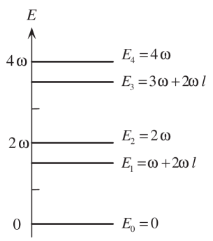
Figure 1: Energy eigenvalues corresponding to eq. (10)

We now focus on the region near $x=0$. In SUSYQM, it is important that the superpotential $W(x,a_{0})$ be a continuous and differentiable function. In our example, the above requirement is satisfied everywhere except at the point $x=0$, where the superpotential of eq. (8) has an infinite discontinuity. Such a discontinuity is not acceptable, and needs regularization. Consider a regularized, continuous superpotential $\widetilde{W}(x,a_{0},\epsilon)$ which reduces to $W(x,a_{0})$ in the limit $\epsilon\to 0$. One such choice is

$$\widetilde{W}(x,a_{0},\epsilon)=W(x,a_{0})~{}f(x,\epsilon)$$ (11)

where

$$f(x,\epsilon)=\tanh^{2}{\frac{x}{\epsilon}}~{}~{}.$$ (12)

The moderating factor $f$ provides a smooth interpolation through the discontinuity, since it is unity everywhere except in a small region of order $\epsilon$ around $x=0$. In this region, $\widetilde{W}(x,a_{0},\epsilon)$ is linear with a slope $l/\epsilon^{2}$. The potential $\widetilde{V}_{-}(x,a_{0},\epsilon)$ corresponding to the superpotential $\widetilde{W}(x,a_{0},\epsilon)$ is

$$\widetilde{V}_{-}(x,a_{0},\epsilon)=\widetilde{W}^{2}(x,a_{0},\epsilon)-\widetilde{W}^{\prime}(x,a_{0},\epsilon)~{}.$$ (13)

In the limit $\epsilon\to 0$, $\widetilde{V}_{-}(x,a_{0},\epsilon)$ reduces to

$$\widetilde{V}_{-}(x,a_{0})=V_{-}(x,a_{0})-4~{}{W}(x,a_{0})~{}\frac{x}{|x|}~{}\delta(x)~{},$$ (14)

where we have used ${\lim}_{\epsilon\to 0}~{}\frac{1}{2\epsilon}{\rm\,sech}^{2}\frac{x}{\epsilon}=\delta(x)$ and ${\lim}_{\epsilon\to 0}~{}\tanh\frac{x}{\epsilon}=\frac{x}{|x|}$. Thus we see that the potential $\widetilde{V}_{-}(x,a_{0})$ has an additional singularity at the origin over ${V}_{-}(x,a_{0})$ given by $\Omega(x)\equiv-4\,l\,\frac{~{}\delta(x)}{|x|}$.

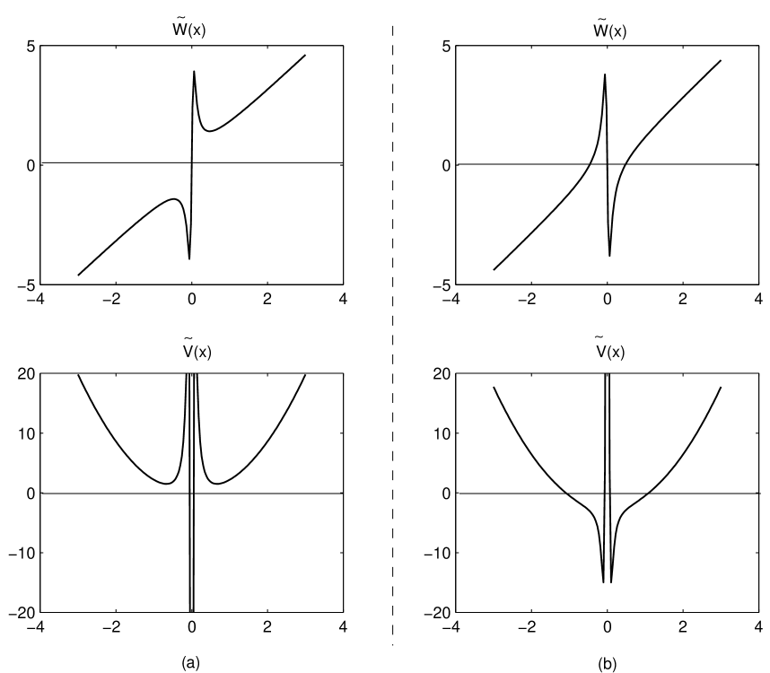
Figure 2: The superpotential $\widetilde{W}$ of eq. (11) and the corresponding potential ${\widetilde{V}_{-}}$ of eq. (13) for the two cases (a) $l\geq 0$ and (b) $l\leq 0$.

Note that in the potential shown in Fig. 2(a), the $\delta$-function singularity is instrumental in producing a bound state at $E_{0}=0$.

Naively, in the limit $\epsilon\to 0$, the potential of eq. (14) appears identical to a three dimensional oscillator with a frequency $\omega$ and angular momentum $l$. However, there are some more subtle but important differences. First, it is defined over the entire real axis ($-\infty<x<\infty$) and not just the half line. For a proper communication between the two halves, we must have a “softness” of the inverse square term. Normalizability of the wave function requires that the coefficient $\lambda$ of the inverse square term be in the transition region $-{1\over 4}<\lambda<3\over 4$ [17]. More specifically, for $(l>0)$, one has $0<l(l+1)<\frac{3}{4}$ and for $(l<0)$ one has $-\frac{1}{4}<l(l+1)<0$. The important special case of the one dimensional harmonic oscillator has $l=0$: it corresponds to $l(l+1)=0$ and no $x^{-2}$ singularity. For transition potentials, both solutions of the Schrödinger equation are square integrable at the origin. Therefore, both are acceptable square integrable solutions of the Schrödinger equation, and must be retained to form a complete set. Eigenstates for the potential $\widetilde{V}_{-}(x,a_{0})$ can be obtained from eq. (6). The lowest four are

$$E_{0}=0;~{}~{}~{}~{} \psi_{0}~{}\propto~{}x^{-l}~{}e^{-{1\over 4}\omega x^{2}}~{},$$

$$E_{1}=(2l+1)\omega;~{}~{}~{} \psi_{1}~{}\propto~{}x^{1+l}~{}e^{-{1\over 4}\omega x^{2}}~{},$$

$$E_{2}=2\omega~{};~{} \psi_{2}~{}\propto~{}\left(2l-1+\omega x^{2}\right)x^{-l}e^{-{1\over 4}\omega x^{2}}~{},$$

$$E_{3}=2\omega+(2l+1)\omega~{}; \psi_{3}~{}\propto~{}\left(-2l-3+\omega x^{2}\right)~{}x^{1+l}~{}e^{-{1\over 4}\omega x^{2}}~{}.$$

General expressions for these eigenfunctions and corresponding eigenenergies are

$$E_{2n}=2n\omega~{},~{}~{}~{}~{}~{}~{} \psi_{2n}\propto x^{-{l}}e^{-{1\over 4}\omega x^{2}}L_{n}^{-l-{1\over 2}}\left[\frac{\omega x^{2}}{2}\right]~{},$$

$$E_{2n+1}=2n\omega+(2l+1)\omega~{},~{} \psi_{2n+1}\propto x^{1+{l}}e^{-{1\over 4}\omega x^{2}}L_{n}^{{l}+{1\over 2}}\left[\frac{\omega x^{2}}{2}\right]~{}~{},$$ (16)

where $L_{n}$ are the standard Laguerre polynomials.

(b) New shape invariant potential obtained from the Pöschl-Teller I potential.

As a second example, we consider the Pöschl-Teller I superpotential

$$W(x,A,B)=A\tan x-B\cot x~{}~{};~{}~{}~{}~{}0<x<\pi/2~{}~{}.$$ (17)

The supersymmetric partner potentials are then given by

$$V_{-}(x,A,B)=A(A-1)\sec^{2}x+B(B-1){\rm\,cosec}^{2}x-(A+B)^{2}~{}~{},$$ (18)

and

$$V_{+}(x,A,B)=A(A+1)\sec^{2}x+B(B+1){\rm\,cosec}^{2}x-(A+B)^{2}~{}~{}.$$ (19)

Here, $A$ and $B$ are both positive in order for $V_{-}(x,A,B)$ to have a zero energy ground state.

Again, one can readily check that there are two possible relations between parameters such that above two potentials exhibit shape invariance. One of them is the conventional $(A\rightarrow A+1,~{}~{}B\rightarrow B+1)$. The second possibility is $(A\rightarrow A+1,~{}~{}B\rightarrow-B)$. As explained in the previous section, this second relationship breaks supersymmetry on $(0,\pi/2)$ domain and it is allowed only if the domain of $x$ is extended to range $-\pi/2<x<\pi/2$. The first transformation among parameters $(A\rightarrow A+1,~{}~{}B\rightarrow B+1)$ has been studied extensively in the literature. It is the second transformation that yields new results and will be considered here. Thus, the relationship among parameters that we consider is, $(A_{k+1}=A_{k}+1,~{}~{}B_{k+1}=-B_{k})$. This potential also requires a careful analysis in the vicinity of $x=0$, where two half-axes are being sewed together. Again, the need of continuity and differentiability of the superpotential requires its regularization, as was done in eq. (11) for the harmonic oscillator. A similar analysis then leads to a new singular shape invariant potential

$$\widetilde{V}_{-}(x,A,B)=\left[A(A-1)\sec^{2}x+B(B-1){\rm\,cosec}^{2}x-(A+B)^{2}\right]+4~{}B\cot x~{}\frac{x}{|x|}~{}\delta(x)~{}.$$ (20)

This potential obeys the shape invariance condition:

$$\widetilde{V}_{+}(x,A,B)=\widetilde{V}_{-}(x,A+1,-B)+(A+1-B)^{2}-(A+B)^{2}~{}~{},$$ (21)

and its eigenvalues and eigenfunctions are given by

$$E_{0}=0~{},$$

$$\psi_{0}\propto\cos^{A}x~{}\sin^{B}x~{},$$

$$E_{1}=(A+1-B)^{2}-(A+B)^{2}~{},$$

$$\psi_{1}\propto\cos^{A}x~{}\sin^{-B-1}x~{}[(2B-1)\cos^{2}x+1]~{},$$

$$E_{2}=(A+2+B)^{2}-(A+B)^{2}~{},$$

$$\psi_{2}\propto\cos^{A}x~{}\sin^{B}x~{}[(4B+2)\cos^{4}x-(6B+3)\cos^{2}x+1]~{},$$

$$E_{3}=(A+3-B)^{2}-(A+B)^{2}~{},$$

$$\psi_{3}\propto\cos^{A}x~{}\sin^{-B-1}x~{}\left[(-8B^{2}+16B-6)\cos^{6}x+(12B^{2}-32B+13)\cos^{4}x+(20B-8)\cos^{2}x+1\right]~{}.$$

Thus, the general formula for eigenvalues is

$$E_{n}=(A+n+(-1)^{n}B)^{2}-(A+B)^{2}~{}~{}.$$ (22)

The eigenspectrum is shown in Fig. 3 and Fig. 4.

Figure 3: The potential of eq. (20) for $A=1.5$ and $B=-1/3$ and its energy spectrum.

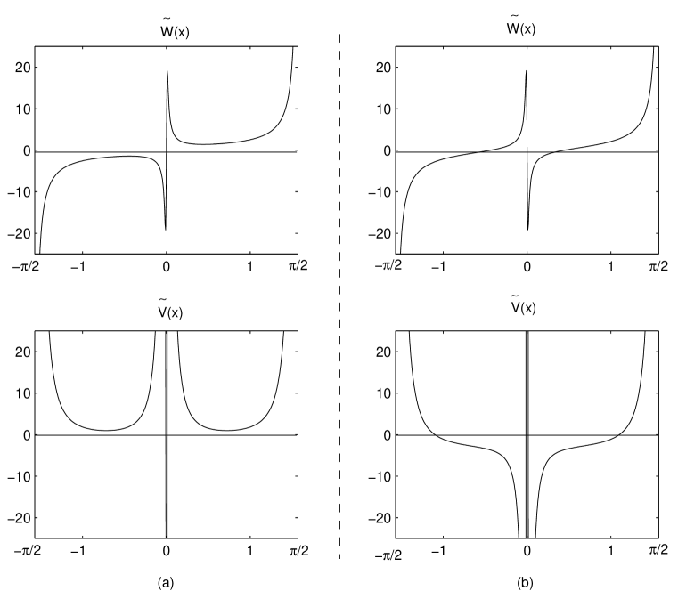
Figure 4: The superpotential $\widetilde{W}$ potential ${\widetilde{V}_{-}}$ from Pöschl-Teller for $A=1.5$ and $B=-1/3$.

Note that, to avoid level crossing, we must have $E_{n}>E_{n-1}$. This leads to the constraint $-\frac{1}{2}<B<\frac{1}{2}$. Interestingly, it is the same constraint that one needs for the normalizability of the wavefunction at the origin and hence to the possibility of communication between regions ($-\frac{1}{2}\pi,0)$ and ($0,\frac{1}{2}\pi)$ of the domain.

(c) New shape invariant potential obtained from the Pöschl-Teller II potential.

The last example that we consider is that of the Pöschl-Teller II potential described by

$$W(x,A,B)=A\tanh x-B\coth x~{}~{};~{}~{}~{}~{}0<x<\infty~{}~{}.$$ (23)

Here, $A$ and $B$ both need to be positive and satisfy the condition $A>B$ for the potential $V_{-}(x,A,B)$ to have a zero energy ground state and to ensure unbroken supersymmetry. The supersymmetric partner potentials are then given by

$$V_{+}(x,A,B)=-A(A-1){\rm\,sech}^{2}x+B(B+1){\rm\,cosec}^{2}x+(A-B)^{2}$$ (24)

and

$$V_{-}(x,A,B)=-A(A+1)\sec^{2}x+B(B-1){\rm\,cosec}^{2}x+(A-B)^{2}~{}~{}.$$ (25)

Here too we have two possible relations between parameters for these potentials to be shape invariant. They are $(A\rightarrow A-1,~{}~{}B\rightarrow B+1)$, and $(A\rightarrow A-1,~{}~{}B\rightarrow-B)$. As explained before in last two examples, the second transformation requires an extension of the range to ($-\infty,\infty$). The new singular potential generated for this case is given by

$$\widetilde{V}_{-}(x,A,B)=\left[-A(A-1){\rm\,sech}^{2}x+B(B+1){\rm\,cosech}^{2}x+(A-B)^{2}\right]+4~{}B\coth x~{}\frac{x}{|x|}~{}\delta(x)~{}.$$ (26)

The shape invariance condition obeyed by this potential is given by

$$\widetilde{V}_{+}(x,A,B)=\widetilde{V}_{-}(x,A+1,-B)+(A-B)^{2}-(A-1+B)^{2}~{}~{},$$ (27)

and the eigenvalues and eigenfunctions are given by

$$E_{0}=0~{},$$

$$\psi_{0}\propto\cosh^{-A}x~{}\sinh^{B}x~{},$$

$$E_{1}=(A-B)^{2}-(A-1+B)^{2}~{},$$

$$\psi_{1}\propto\cosh^{-A}x~{}\sinh^{-B-1}x~{}[(2B-1)\cosh^{2}x+1]~{},$$

$$E_{2}=(A-B)^{2}-(A-2-B)^{2}~{},$$

$$\psi_{2}\propto\cosh^{A}x~{}\sinh^{B}x~{}[(4B+2)\cosh^{4}x-(6B+3)\cosh^{2}x+1]~{},$$

$$E_{3}=(A-B)^{2}-(A-3+B)^{2}~{},$$

$$\psi_{3}\propto\cosh^{A}x~{}\sinh^{-B-1}x~{}\left[(8B^{2}-16B+6)\cosh^{6}x-(12B^{2}-32B+13)\cosh^{4}x\right.$$

$$\left.\hskip 180.67499pt-(20B-8)\cosh^{2}x-1\right]~{}.$$ (28)

Thus, the general formula for eigenvalues is

$$E_{n}=(A-B)^{2}-(A-n-(-1)^{n}B)^{2}~{}~{}.$$ (29)

Again, to steer clear of the level crossing problem, we must have $E_{n}>E_{n-1}$. This leads to the constraint $-\frac{1}{2}<B<\frac{1}{2}$; which, as stated earlier, is the same constraint that one needs for the normalizability of the wavefunction at the origin and for an effective communication between two halves of the $x$-axis.

4. Potential Algebra:

So far, we have discussed three types of new solvable singular potentials. We will now derive the potential algebra underlying them. We will show that the algebra based on the generators $\{J_{+},J_{-},J_{3}\}$ is non-linear [6, 7, 8, 9, 10] . Potential algebras provide an alternative way of getting the eigenvalues by algebraic means.

Consider the following ansatz:

$$J_{+}=c^{-1}\,{\cal A}^{\dagger}\left(x,\alpha(N),\beta(N)\right)~{}~{},~{}~{}J_{-}={\cal A}\left(x,\alpha(N),\beta(N)\right)c~{}~{},~{}~{}J_{3}=N\equiv c^{\dagger}c~{}~{},$$ (30)

where $c,c^{\dagger}$ and $c^{-1}$ are three operators satisfying $[c,c^{\dagger}]=1$, and $c\,c^{-1}=c^{-1}\,c=1$. An example of such operators is given by $c=e^{i\phi},~{}c^{-1}=e^{-i\phi}$ and $c^{\dagger}=i\partial_{\phi}\,e^{-i\phi}$, where $\phi$ is some arbitrary real variable. The operators ${\cal A}$ and ${\cal A}^{\dagger}$ of eq. ( 30) are obtained from eq. (2) via the substitution $a_{0}\equiv\{A,B\}\rightarrow\{\alpha(N),\beta(N)\}$, where $\alpha$ and $\beta$ are real, arbitrary functions to be determined later. We can readily check that

$$[J_{3},J_{\pm}]=\pm J_{\pm}~{},~{}[J_{+},J_{-}]=-R(J_{3})\equiv g(\alpha(N),\beta(N))-g(\alpha(N-1),\beta(N-1))~{}.$$ (31)

The last commutation relation is a consequence of the algebraic shape invariance condition [9]

$$H_{+}(x,\alpha(N),\beta(N))-H_{-}\,(x,\alpha(N-1),\beta(N-1))=g(\alpha(N-1),\beta(N-1))-g(\alpha(N),\beta(N))~{},$$ (32)

which is the operatorial “twin” of the classical shape invariance condition eq. (4) obtained via the mappings $\{A_{0},B_{0}\}\rightarrow\{\alpha(N),\beta(N)\}$ and respectively $\{A_{1},B_{1}\}\rightarrow\{\alpha(N-1),\beta(N-1)\}$.

The functions $\alpha(N)$ and $\beta(N)$ are determined by requiring that the change $\alpha(N)\rightarrow\alpha(N-1)$ and $\beta(N)\rightarrow\beta(N-1)$ correspond to the change of parameters $a_{0}\rightarrow a_{1}$. For example, $\alpha(N)=A-N$ corresponds to a translational change of parameters $A_{0}\rightarrow A_{1}=A_{0}+1$, because $\alpha(N-1)=\alpha(N)+1$. Similarly, $\beta(N)=(-1)^{N}$ corresponds to the reflection $B_{0}\rightarrow B_{1}=-B_{0}~{}$, since $~{}\beta(N-1)=-\beta(N)$.

For any shape invariant potential, we know the function $g(\alpha,\beta)$, which explicitly gives the potential algebra (31). From its representations, we can obtain the energy spectrum for the given problem.

To find a representation of the potential algebra, let us consider a set of eigenvectors common to both $H_{-}=J_{+}J_{-}$ and $J_{3}=N$ denoted by $\{|n\rangle,n=0,1,\ldots\}$. The action of $J_{+},~{}J_{-}$ and $J_{3}$ on this basis is given by

$$J_{+}|n\rangle=a(n+1)|n+1\rangle~{},~{}~{}J_{-}|n\rangle=a(n)|n-1\rangle~{},~{}~{}J_{3}|n\rangle=n|n\rangle~{}~{}.$$ (33)

Here we have chosen, without any loss of generality, the coefficients $a(n)$ to be real. Note that since $J_{-}|0\rangle=0$, we have the initial condition $a(0)=0$. There is a connection between the coefficients $a(n)$ and the eigenspectrum of the Hamiltonian. Observe that

$$H_{-}(x,\alpha(N-1),\beta(N-1))\,|n\rangle=J_{+}J_{-}|n\rangle=a^{2}(n)|n\rangle~{}.$$ (34)

Therefore, in order to find the spectrum of the Hamiltonian we have to determine the coefficients $a^{2}(n)$. This can be done by projecting the last equation from (31) on $|n\rangle$ and solving the resulting equation recursively. Thus, we obtain $a^{2}(n)-a^{2}(n+1)=g(n)-g(n-1)$ having the solution $a^{2}(n)=g(-1)-g(n-1)$. Here we have denoted $g(n)\equiv g(\alpha(n),\beta(n))$. But $a^{2}(n)$ corresponds to the eigenvalues of the Hamiltonian $H_{-}(x,\alpha(N-1),\beta(N-1))$, or “classically” speaking to the shifted set parameters $a_{1}$. Therefore the eigenenergies of the initial Hamiltonian $H_{-}(x,\alpha(N),\beta(N))$ (corresponding to the set of parameters $a_{0}$) are

$$E_{n}=g(\alpha(0),\beta(0))-g(\alpha(n),\beta(n))~{}.$$ (35)

We make contact with eq. (6) by observing that $\{\alpha(n-k),\beta(n-k)\}\equiv a_{k}$.

(a) The harmonic oscillator.

To show how our procedure works, it is instructive to build explicitly the potential algebra of the harmonic oscillator. The superpartner potentials $V_{-}$ and $V_{+}$ are given in eqs. (7) and respectively (9). Under the change of parameters $\{l,\omega\}\rightarrow\{l-1,\omega\}$ we have the following shape invariance condition

$$H_{+}(x,l,\omega)=H_{-}(x,l-1,\omega)+(-2\omega\,(l-1))-(-2\omega\,l)~{}.$$

To build the potential algebra, first we find the functions $\alpha$ and $\beta$ associated with the above change of parameters. We have immediately $\alpha(N)=l+N~{},~{}~{}\beta(N)=\omega$. Next, we can build the concrete realization of the potential algebra using the ansatz (30) and the superpotential from (8). The resulting generators

$$J_{+}=c^{-1}\,\left(-\frac{d}{dx}+\frac{1}{2}\,x\,\omega+\frac{l+N}{x}\right)~{},~{}~{}J_{-}=\left(\frac{d}{dx}+\frac{1}{2}\,x\,\omega+\frac{l+N}{x}\right)\,c~{},~{}~{}J_{3}=N\equiv c^{\dagger}c~{},$$ (36)

satisfy the “canonical” commutation relations (31), where the function $g$ is given by $g(N)\equiv g(\alpha(N),\beta(N))=-2\omega\,(l+N)$. Finally, using the formula (35) we get the spectrum $E_{n}=g(0)-g(n)=2\omega\,n$, which is exactly what we have expected.

Next, let us consider the new singular shape invariant potential corresponding to the change of parameters $\{l,\omega\}\rightarrow\{-l,\omega\}$. In this case $\alpha(N)=-(-1)^{N}l$ and $\beta(N)=\omega$. From eq. (30) we get

$$J_{+}=c^{-1}\,\left(-\frac{d}{dx}+\frac{1}{2}\,x\,\omega-\frac{(-1)^{N}l}{x}\right)~{},~{}~{}J_{-}=\left(\frac{d}{dx}+\frac{1}{2}\,x\,\omega-\frac{(-1)^{N}l}{x}\right)\,c~{},~{}~{}J_{3}=N\equiv c^{\dagger}c~{}.$$ (37)

The commutation relations (31) together with the algebraic shape invariance condition (32) yield in this case $[J_{+},J_{-}]=-\omega\,(-2(-1)^{N}l+1)$ from where we get $g(N)=\omega\,((-1)^{N}l-N)$. Therefore, the resulting eigenspectrum (35) is $E_{n}=\omega\,n+\omega\,l\,(1-(-1)^{n})$.

(b) The Pöschl-Teller I potential.

We build the algebraic model for the new shape invariant Pöschl-Teller I like potential by taking into account that corresponding to the change of parameters $\{A,B\}\rightarrow\{A+1,-B\}$ we have $\alpha(N)=A-N$ and $\beta(N)=(-1)^{N}B$. Then, using the superpotential (17) one gets the following expressions for the generators of the associate potential algebra

$$J_{+}\!\!\!\! = \!\!\!\!c^{-1}\,\left(-\frac{d}{dx}+(A-N)\tan x-(-1)^{N}B\cot x\right)~{},$$

$$J_{-}\!\!\!\! = \!\!\!\!\left(-\frac{d}{dx}+(A-N)\tan x-(-1)^{N}B\cot x\right)\,c~{},~{}~{}J_{3}=N\equiv c^{\dagger}c~{}.$$ (38)

Using as before the algebraic shape invariance condition (32) we obtain in this case $[J_{+},J_{-}]=-(A+N+1+(-1)^{(N+1)}B)^{2}+(A+N+(-1)^{N}B)^{2}$. Therefore we get $g(N)=-(A+N+(-1)^{N}B)^{2}$ and the corresponding eigenspectrum $E_{n}=g(0)-g(n)=-(A+B)^{2}+(A-n+(-1)^{n}B)$.

(c) The Pöschl-Teller II potential.

For the new the Pöschl-Teller II potential like case, to the change of parameters $\{A,B\}\rightarrow\{A-1,-B\}$ we have $\alpha(N)=-(A-N)$ and $\beta(N)=(-1)^{N}B$ and the corresponding algebra is therefore generated by

$$J_{+}\!\!\!\! = \!\!\!\!c^{-1}\,\left(-\frac{d}{dx}+(-A+N)\tanh x-(-1)^{N}B\coth x\right)~{},$$

$$J_{-}\!\!\!\! = \!\!\!\!\left(-\frac{d}{dx}+(-A+N)\tanh x-(-1)^{N}B\coth x\right)\,c~{},~{}~{}J_{3}=N\equiv c^{\dagger}c~{}.$$ (39)

In the above representation the explicit form of the superpotential (23) was taken into account. The commutation relations (31) together with the algebraic shape invariance condition (32) yield in this case $g(N)=(-A+N-(-1)^{N}B)^{2}$. Using (35), one obtains as expected, the eigenspectrum for this potential $E_{n}=g(0)-g(n)=(A+B)^{2}-(-A+n-(-1)^{n}B)^{2}$.

5. Conclusions and Comments:

We have generated several new shape invariant potentials on the whole line starting from well known potentials on the half line. To ensure continuity and differentiability of the superpotential, our procedure requires a regularisation at the origin. This extension not only maintains shape invariance, it also allows the possibility of a new transformation among parameters ($B\rightarrow-B$) that was not allowed on the half-axis. This transformation results in new superpotentials, albeit singular, that are defined over the entire real axis and have richer spectra than those defined over half-axis. It is shown further that the eigenspectra of these new real singular shape invariant potentials may also be derived from a nonlinear potential algebra.

Since we have obtained and discussed the exact eigenvalues and eigenfunctions of three new singular potentials using the machinery of supersymmetric quantum mechanics, it is of interest to ask what one gets in the WKB approximation. Let us recall that Comtet et al. have shown the exactness of the SWKB quantization condition[18, 13]

$$\int_{x_{1}}^{x_{2}}\sqrt{E_{n}-W^{2}}~{}dx=n\pi\hbar~{}~{}.$$

for all known shape invariant problems with unbroken SUSY where parameters are related by $a_{1}=a_{0}+\delta$ [21].

For broken SUSY, Inomata and Junker[19] gave the quantization condition

$$\int_{x_{1}}^{x_{2}}\sqrt{E_{n}-W^{2}}~{}dx\!\!\!\! = \!\!\!\![n+1/2]\pi\hbar~{}~{}.$$

For both cases, the turning points $x_{1},x_{2}$ are solutions of $W^{2}(x)=E_{n}$.

Our new singular potentials allow a change of parameters that, if considered in half-axes only, leads the system to alternate through unbroken and broken phases of supersymmetry as $a_{k}\rightarrow a_{k+1}$. It is interesting to note that the spectrum of these singular potentials can be derived, using somewhat more complex but exact quantization condition which alternates between the broken and unbroken SUSY cases:

$$\int_{x_{1}}^{x_{2}}\sqrt{E_{n}-W^{2}}~{}dx\!\!\!\! = \!\!\!\![n+{1/2}P_{n}]~{}~{},$$

where $P_{n}$ is equal to $[1-(-1)^{n}]/2$.

Partial financial support from the U.S. Department of Energy is gratefully acknowledged. R.D. would like to thank the Department of Atomic Energy, Government of India for a research grant, and the Physics Department of the University of Illinois at Chicago for warm hospitality.

Appendix A:  In this appendix, we show that shape invariance of our new potentials is maintained during the process of extending the domain to the whole real axis and introducing the moderating factor $f(x,\epsilon)$. Let us recall that our old superpotential $W(x,A,B)$ is of the form $A~{}\Phi(x)+B~{}\left[\Phi(x)\right]^{-1}$, where the function $\Phi(x)$ is $x,\tan x$ or $\tanh x$ for harmonic oscillator, Pöschl-Teller I, and Pöschl-Teller II respectively

Note that in all cases, $\left[\Phi(x)\right]^{-1}\longrightarrow 1/x$ at the origin. $W(x,A,B)$ is replaced by a regularized, continuous superpotential $\widetilde{W}(x,A,B,\epsilon)$ given by

$$\widetilde{W}(x,A,B,\epsilon)=W(x,A,B)~{}f(x,\epsilon)~{},$$ (41)

where $f(x,\epsilon)$ is unity everywhere except in a small region of order $\epsilon$ around $x=0$. One such function $f(x,\epsilon)$ is given by $\tanh^{2}\left(x/\epsilon\right)$. In the limit $\epsilon\rightarrow 0$, we assume that the $f(x,\epsilon)\rightarrow 1$ and $\frac{df(x,\epsilon)}{dx}\rightarrow 2\frac{x}{|x|}\delta(x)$. The potentials $\widetilde{V}_{\mp}(x,A,B,\epsilon)$ corresponding to the superpotential $\widetilde{W}(x,A,B,\epsilon)$ are then given by

$$\widetilde{V}_{\mp}(x,A,B,\epsilon)=W^{2}(x,A,B)f^{2}(x,\epsilon)\mp\left(\frac{dW(x,A,B)}{dx}~{}f(x,\epsilon)+\frac{df(x,\epsilon)}{dx}~{}W(x,A,B)\right)~{}~{}.$$

Now

$$\widetilde{V}_{+}(x,A,B,\epsilon)-\widetilde{V}_{-}(x,\widetilde{A},\widetilde{B},\epsilon)\!\!\!\! = \!\!\!\!V_{+}(x,A,B)-V_{-}(x,\widetilde{A},\widetilde{B})+\frac{df(x,\epsilon)}{dx}~{}\left(W(x,A,B)~{}+~{}W(x,\widetilde{A},\widetilde{B})\right)$$ (42)

$$= \!\!\!\!R(A,B)+\frac{df(x,\epsilon)}{dx}~{}\left(B+\widetilde{B}\right)\left[\Phi(x)\right]^{-1}$$

$$= \!\!\!\!R(A,B)~{}~{},$$

where we have used the limits of $f$ and $f^{\prime}$ and $\widetilde{B}=-B$. This establishes the shape invariance of the regularized superpotential.

References

[1]
C. M. Bender, S. Boettcher, Phys. Rev. Lett. 24, (1998) 5243;
F. Cannata, G. Junker and J. Trost, Phys. Lett. A 246, (1998) 219;
C. M. Bender, S. Boettcher and P.N. Meisinger, J. Math. Phys. 40, (1999) 2201;
A. A. Andrianov, M. V. Ioffe, F. Cannata and J. P. Dedonder, Int. J. Mod. Phys. A 14, (1999) 2675;
M. Znojil, Phys. Lett. A. 264, (1999) 108;
M. Znojil, J. Phys. A: Math. Gen. A 32, (1999) 4563;
B. Bagchi and C. Quesne, Phys. Lett. A 273, (2000) 285.
[2] M. Znojil, Phys. Lett. A 259, (1999) 220;
G. Levai and M. Znojil, Phys. J. Phys. A 33, (2000) 7165.
[3] M. Znojil, arXiv: quant-ph/9911116.
[4] A. Gangopadhyaya and U. Sukhatme, Phys. Lett. A 224, (1996) 5.
[5]
L. Infeld and T.E. Hull, Rev. Mod. Phys., 23, (1951) 21 ;
L. E. Gendenshtein, Pismah. Eksp. Teor. Fiz. 38, 299 (1983) [JETP Lett., 38, (1983) 356 ];
L. E. Gendenshtein and I. V. Krive, Sov. Phys. Usp. 28, (1985) 645.
[6] J. Wu and Y. Alhassid, Phys. Rev. A 31, (1990) 557;
H. Y. Cheung, Nuovo Cimento B 101, (1988) 193.
[7]J. Wu, Y. Alhassid and F. Gürsey Ann. Phys. 196, 163 (1989).
[8]A. Gangopadhyaya, J.V. Mallow and U.P. Sukhatme,
Proceedings of Workshop on Supersymmetric Quantum Mechanics and Integrable
Models, June 1997, Editor: Henrik Aratyn et al., Publisher by Springer-Verlag.
[9]A. Gangopadhyaya, J.V. Mallow and
U.P. Sukhatme, Phys. Rev. A 58, 4287 (1998),
S. Chaturvedi, R. Dutt, A. Gangopadhyaya, P. Panigrahi, C. Rasinariu, U. Sukhatme, Phys. Lett. A 248, (1998)109.
R.Dutt, A. Gangopadhyaya, C. Rasinariu and
U.Sukhatme, Phys. Rev. A 60, (1999) 3482.
[10]A.B. Balantekin, Phys. Rev. A 57, (1998) 4188
; (quant-ph/9712018).
[11] E. Witten, Nucl. Phys. B 188, (1981) 513;
F. Cooper and B. Freedman, Ann. Phys. (N.Y.) 146, (1983) 262;
C.V.Sukumar, J. Phys. A: Math. Gen. 18, (1985) 2917.
[12]
F. Cooper, A. Khare and U. Sukhatme, Phys. Rep. 251, (1995) 268,
and references therein.
[13]R. Dutt, A. Khare, and U. Sukhatme, Am. J. Phys. 56,
(1988) 163.
[14] A. Khare and U. Sukhatme, Jour. Phys. A21, (1988) L501.
[15] R. Dutt, A. Khare and U. Sukhatme, Phys. Lett. 181B,
(1986) 295.
[16]D. Barclay, R. Dutt, A. Gangopadhyaya, A. Khare,
A. Pagnamenta and U. Sukhatme, Phys. Rev. A 48, (1993) 2786.
[17] A. Gangopadhyaya, P. K. Panigrahi and U. P. Sukhatme, J. Phys. A 27, (1994) 4295;
L. D. Landau and E. M. Lifshitz, Quantum Mechanics,
Pergamon Press (1977);
W. M. Frank, D. J. Land and R. M. Spector, Rev. Mod. Phys. 43, (1971) 36.
[18] A. Comtet, A. D. Bandrauk and D. K. Campbell, Phys. Lett. B 150, (1985) 159.
[19] A. Inomata and G. Junker, in Proc. Adriatic Research Conf.
on Path-integration and its applications, 3-6 September 1991, ITCTP, Trieste.
[20]R. Dutt, A. Gangopadhyaya, A. Khare, A. Pagnamenta, and U. Sukhatme; Phys. Lett. 174 A, 2854 (1993).
[21]D.T. Barclay, A. Khare, and U. Sukhatme, Phys. Lett. A 183, (1993) 263.